Identification of Linear and Bilinear Systems: A Unified Study

Abstract

System identification problems are always challenging to address in applications that involve long impulse responses, especially in the framework of multichannel systems. In this context, the main goal of this review paper is to promote some recent developments that exploit decomposition-based approaches to multiple-input/single-output (MISO) system identification problems, which can be efficiently solved as combinations of low-dimension solutions. The basic idea is to reformulate such a high-dimension problem in the framework of bilinear forms, and to then take advantage of the Kronecker product decomposition and low-rank approximation of the spatiotemporal impulse response of the system. The validity of this approach is addressed in terms of the celebrated Wiener filter, by developing an iterative version with improved performance features (related to the accuracy and robustness of the solution). Simulation results support the main theoretical findings and indicate the appealing performance of these developments.

1. Introduction

Solving a system identification problem represents a key step in many important real-world applications [1,2]. In general, such a problem can be formulated in terms of estimating or modeling the parameters of an unknown system when a set of data is available, which is usually related to the input and output of the system. Depending on the specific particularities of the problem or application, we can deal with different types of systems, according to their numbers of inputs and outputs. The simplest formulation is the well-known single-input/single-output (SISO) system. Furthermore, in some applications we can deal with more elaborated structures, such as multiple-input/single-output (MISO) and multiple-input/multiple-output (MIMO) systems.

The linearity is an important feature of a system, which can significantly simplify the overall identification problem. Even if many real-world systems face nonlinear behaviors, it is always desirable to address or reformulate the framework such that it has a linear approach to some extent. In this context, a useful topic is related to bilinear forms, which have been addressed in the literature in different ways and contexts [3,4,5,6,7,8,9,10,11,12,13,14,15,16,17,18,19,20,21,22]; most often they are related to approximating nonlinear systems.

In general, a bilinear model can approximate a large class of nonlinear systems via a finite sum of the Volterra series expansion between the inputs and outputs of the system. Therefore, in this context, bilinear systems behave similarly (to some extent) to linear models. This could further simplify the analysis, as outlined before. Due to this simplicity, bilinear systems have been involved in a wide range of applications, such as digital filter synthesis [7], prediction problems [8], channel equalization [9], echo cancellation [10], chaotic communications [16], neural networks [20], and active noise control [21]. Nevertheless, in all these frameworks, the bilinear term is defined with respect to the data, i.e., in terms of an input-output relation.

In this study, we focus on a different approach by defining the bilinear term with respect to the impulse responses of a spatiotemporal model, in the context of MISO systems. Several similar frameworks can be found in the literature, in the context of particular applications, such as channel equalization [13], nonlinear acoustic echo cancellation [15], and target detection [18]. However, most of these works were not associated with or analyzed in conjunction with bilinear forms. Usually, they were referred to as joint adaptation processes or cascaded systems, which are similar to the Hammerstein model [23].

More recently, an iterative Wiener filter for such bilinear forms was developed in the framework of a MISO system identification problem [24]. As compared to the conventional Wiener filter, the iterative version can obtain good accuracy even when a only small amount of information is available for the estimation of the statistics. Following the Wiener benchmark, another category of solutions relies on adaptive filtering [25,26]. Several adaptive filters tailored for the identification of bilinear forms have also been developed, following the main categories of algorithms. For example, the least-mean-square (LMS) and normalized LMS (NLMS) versions can be found in [27,28]. In addition, several recursive least-squares (RLS) algorithms for bilinear forms were developed in [29]. Moreover, a Kalman filter tailored for the identification of bilinear forms was proposed in [30].

In the previously mentioned approaches, the spatiotemporal impulse response of the MISO system is considered perfectly separable, and its components are combined using the Kronecker product. The identification of such linearly separable systems can be efficiently exploited in the frameworks of different applications, such as source separation [31,32], array beamforming [33,34], and object recognition [35,36]. In these contexts, the basic solution relies on the decomposition and modeling techniques of rank-1 tensors [37,38,39,40,41,42]. Nevertheless, it is highly useful to exploit the decomposition-based approach for the identification of more general forms of impulse responses.

Several recent works have followed this idea by exploiting the nearest Kronecker product decomposition and low-rank approximations [43,44,45,46,47]. In this context, the basic concept is to reformulate a high-dimension system identification problem as a combination of low-dimension solutions, thereby gaining in terms of both performance and complexity. Due to its features, this approach can be used in different practical applications—e.g., [48,49,50,51,52,53,54,55], among which we can mention acoustic feedback cancellation, adaptive beamforming, speech dereverberation, multichannel linear prediction, and nonlinear system identification.

A unified study on the efficient identification of linear and bilinear systems exploiting the decomposition-based approach is provided in this review paper. First, in Section 2, we present different system models, in the context of linear and bilinear forms. Then, in Section 3, we show how these models are related, thereby outlining the equivalence among the systems. The ideas behind the decomposition-based approach together with the optimal low-rank approximation are presented in Section 4. Since the Wiener filter represents a benchmark tool for the system identification problems, we illustrate its behavior in Section 5, wherein we also introduce an iterative version with improved performance features. Simulation results are provided in Section 6, in order to support the main theoretical findings. Finally, several conclusions and perspectives of this study are outlined in Section 7.

2. Different Input Output Linear/Bilinear System Models

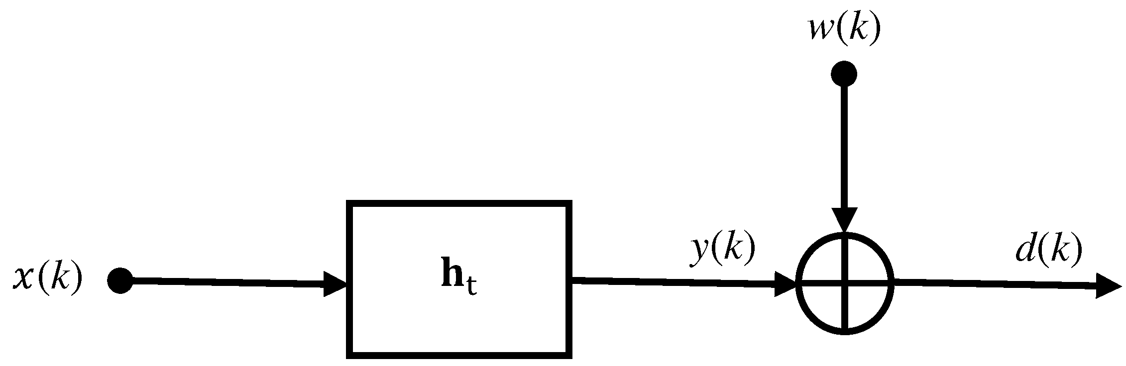
In this study, we assume that the input and output, and the noise signals, take real values and have zero means. The most popular input output system is the so-called SISO system given by

$$\begin{array}{cc}\hfill d\left(k\right)& ={\mathbf{h}}_{\mathrm{t}}^T\mathbf{x}\left(k\right)+w\left(k\right)\hfill \\ \hfill & =y\left(k\right)+w\left(k\right),\hfill \end{array}$$

(1)

where $d\left(k\right)$ denotes the desired (or reference) signal at discrete-time index k, ${\mathbf{h}}_{\mathrm{t}}$ is the system’s temporal impulse response of length L, and the superscript ${}^T$ denotes the transpose operator. The vector

$$\begin{array}{cc}\hfill \mathbf{x}\left(k\right)& ={\left[\begin{array}{cccc}x\left(k\right)& x(k-1)& \cdots & x(k-L+1)\end{array}\right]}^T\hfill \end{array}$$

(2)

contains the most recent L samples of the input signal, $x\left(k\right)$; $w\left(k\right)$ is the additive noise; and $y\left(k\right)={\mathbf{h}}_{\mathrm{t}}^T\mathbf{x}\left(k\right)$ is the linear form in ${\mathbf{h}}_{\mathrm{t}}$. A typical assumption that can be made is that $x\left(k\right)$ and $w\left(k\right)$ are uncorrelated (or even independent, which is not really required if we only handle second-order statistics). We refer to (1) as the linear SISO (LSISO) system. Its general block diagram is provided in Figure 1.

Without loss of generality, let us assume that $L=L_1{L}_2$, with $L_1\ge L_2$. A shorter version of the input signal vector, $\mathbf{x}\left(k\right)$, may be written as

$$\begin{array}{cc}\hfill {\mathbf{x}}^{\prime }\left(k\right)& ={\left[\begin{array}{cccc}x\left(k\right)& x(k-1)& \cdots & x(k-L_1+1)\end{array}\right]}^T.\hfill \end{array}$$

(3)

As a result, we can express (2) as

$$\begin{array}{cc}\hfill \mathbf{x}\left(k\right)& ={\left[\begin{array}{cccc}{\mathbf{x}}^{\prime T}\left(k\right)& {\mathbf{x}}^{\prime T}(k-L_1)& \cdots & {\mathbf{x}}^{\prime T}[k-(L_2-1)L_1]\end{array}\right]}^T,\hfill \end{array}$$

(4)

from which we deduce the matrix of size $L_1\times L_2$:

$$\begin{array}{cc}\hfill \mathbf{X}\left(k\right)& =\left[\begin{array}{cccc}{\mathbf{x}}^{\prime }\left(k\right)& {\mathbf{x}}^{\prime }(k-L_1)& \cdots & {\mathbf{x}}^{\prime }[k-(L_2-1)L_1]\end{array}\right].\hfill \end{array}$$

(5)

In other terms, we have

$$\begin{array}{cc}\hfill \mathbf{x}\left(k\right)& =\mathrm{vec}\left[\mathbf{X}\left(k\right)\right],\hfill \end{array}$$

(6)

where $\mathrm{vec}[·]$ denotes vectorization, i.e., the operation of converting a matrix into a vector. It may also be convenient to use the inverse of the vectorization operator [40], i.e., $\mathbf{X}\left(k\right)=\mathrm{ivec}\left[\mathbf{x}\left(k\right)\right]$, which is equivalent to (6). Therefore, the most straightforward bilinear system that follows from the previous development results as

$$\begin{array}{cc}\hfill d\left(k\right)& ={\mathbf{h}}_{\mathrm{t}1}^T\mathbf{X}\left(k\right){\mathbf{h}}_{\mathrm{t}2}+w\left(k\right)\hfill \\ \hfill & =y\left(k\right)+w\left(k\right),\hfill \end{array}$$

(7)

where ${\mathbf{h}}_{\mathrm{t}1}$ and ${\mathbf{h}}_{\mathrm{t}2}$ are the first and second temporal impulse responses, of lengths $L_1$ and $L_2$, respectively; and $y\left(k\right)={\mathbf{h}}_{\mathrm{t}1}^T\mathbf{X}\left(k\right){\mathbf{h}}_{\mathrm{t}2}$ is now bilinear in ${\mathbf{h}}_{\mathrm{t}1}$ and ${\mathbf{h}}_{\mathrm{t}2}$. We call (7) the bilinear SISO (BSISO1) system. The equivalency between the LSISO and BSISO1 systems is explained and detailed in Section 3, together with the connections among different models that are discussed in the current section.

An obvious generalization of (7) is

$$\begin{array}{cc}\hfill d\left(k\right)& =\sum _{l=1}^{L_2}{\mathbf{h}}_{\mathrm{t}1,l}^T\mathbf{X}\left(k\right){\mathbf{h}}_{\mathrm{t}2,l}+w\left(k\right),\hfill \end{array}$$

(8)

where ${\mathbf{h}}_{\mathrm{t}1,l},l=1,2,\dots ,L_2$ and ${\mathbf{h}}_{\mathrm{t}2,l},l=1,2,\dots ,L_2$ are the first and second sets of the system temporal impulse responses of lengths $L_1$ and $L_2$, respectively. We refer to (8) as the BSISO2 system. Expression (8) can be rewritten as

$$\begin{array}{cc}\hfill d\left(k\right)& ={\mathit{h}}_{\mathrm{t}1}^T\mathit{X}\left(k\right){\mathit{h}}_{\mathrm{t}2}+w\left(k\right)\hfill \\ \hfill & =y\left(k\right)+w\left(k\right),\hfill \end{array}$$

(9)

where

$$\begin{array}{cc}\hfill {\mathit{h}}_{\mathrm{t}1}& ={\left[\begin{array}{cccc}{\mathbf{h}}_{\mathrm{t}1,1}^T& {\mathbf{h}}_{\mathrm{t}1,2}^T& \cdots & {\mathbf{h}}_{\mathrm{t}1,L_2}^T\end{array}\right]}^T,\hfill \end{array}$$

(10)

$$\begin{array}{cc}\hfill {\mathit{h}}_{\mathrm{t}2}& ={\left[\begin{array}{cccc}{\mathbf{h}}_{\mathrm{t}2,1}^T& {\mathbf{h}}_{\mathrm{t}2,2}^T& \cdots & {\mathbf{h}}_{\mathrm{t}2,L_2}^T\end{array}\right]}^T,\hfill \end{array}$$

(11)

and

$$\begin{array}{cc}\hfill \mathit{X}\left(k\right)& =\mathrm{bdiag}\left[\mathbf{X}\left(k\right),\mathbf{X}\left(k\right),\dots ,\mathbf{X}\left(k\right)\right]\hfill \end{array}$$

(12)

is a block-diagonal matrix with $L_2$ diagonal blocks. We can see that $y\left(k\right)={\mathit{h}}_{\mathrm{t}1}^T\mathit{X}\left(k\right){\mathit{h}}_{\mathrm{t}2}$ is bilinear in ${\mathit{h}}_{\mathrm{t}1}$ and ${\mathit{h}}_{\mathrm{t}2}$.

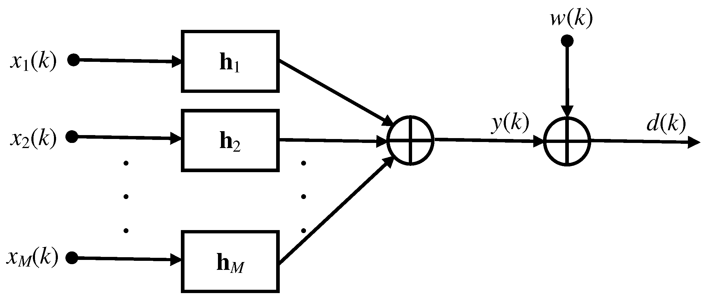
An important extension of the LSISO system in (1) is the so-called linear MISO (LMISO) system:

$$\begin{array}{cc}\hfill d\left(k\right)& =\sum _{m=1}^M{\mathbf{h}}_m^T{\mathbf{x}}_m\left(k\right)+w\left(k\right),\hfill \end{array}$$

(13)

where M denotes the number of system inputs (or channels), ${\mathbf{h}}_m,m=1,2,\dots ,M$ are the M channel impulse responses of length L, and the vector

$$\begin{array}{cc}\hfill {\mathbf{x}}_m\left(k\right)& ={\left[\begin{array}{cccc}{x}_m\left(k\right)& x_m(k-1)& \cdots & x_m(k-L+1)\end{array}\right]}^T\hfill \end{array}$$

(14)

contains the most recent L samples of the mth ($m=1,2,\dots ,M$) input signal, $x_m\left(k\right)$. The general block diagram of the LMISO system is provided in Figure 2. Equation (13) can be rewritten as

$$\begin{array}{cc}\hfill d\left(k\right)& ={\overline{\mathbf{h}}}^T\overline{\mathbf{x}}\left(k\right)+w\left(k\right)\hfill \\ \hfill & =y\left(k\right)+w\left(k\right),\hfill \end{array}$$

(15)

where

$$\begin{array}{cc}\hfill \overline{\mathbf{h}}& ={\left[\begin{array}{cccc}{\mathbf{h}}_1^T& {\mathbf{h}}_2^T& \cdots & {\mathbf{h}}_M^T\end{array}\right]}^T,\hfill \end{array}$$

(16)

$$\begin{array}{cc}\hfill \overline{\mathbf{x}}\left(k\right)& ={\left[\begin{array}{cccc}{\mathbf{x}}_1^T\left(k\right)& {\mathbf{x}}_2^T\left(k\right)& \cdots & {\mathbf{x}}_M^T\left(k\right)\end{array}\right]}^T.\hfill \end{array}$$

(17)

Clearly, $y\left(k\right)={\overline{\mathbf{h}}}^T\overline{\mathbf{x}}\left(k\right)$ is linear in $\overline{\mathbf{h}}$. Of course, the particular case of $M=1$ corresponds to the LSISO system.

As in the single-channel case, let $L=L_1{L}_2$ but with $M{L}_1\ge L_2$. We can decompose ${\mathbf{x}}_m\left(k\right)$, similarly to (4), as

$$\begin{array}{cc}\hfill {\mathbf{x}}_m\left(k\right)& ={\left[\begin{array}{cccc}{\mathbf{x}}_m^{\prime T}\left(k\right)& {\mathbf{x}}_m^{\prime T}(k-L_1)& \cdots & {\mathbf{x}}_m^{\prime T}[k-(L_2-1)L_1]\end{array}\right]}^T,\hfill \end{array}$$

(18)

where

$$\begin{array}{cc}\hfill {\mathbf{x}}_m^{\prime }\left(k\right)& ={\left[\begin{array}{cccc}{x}_m\left(k\right)& x_m(k-1)& \cdots & x_m(k-L_1+1)\end{array}\right]}^T.\hfill \end{array}$$

(19)

Then, we concatenate the M input signals as

$$\begin{array}{cc}\hfill \underline{\mathbf{x}}\left(k\right)& ={\left[\begin{array}{cccc}{\underline{\mathbf{x}}}^{\prime T}\left(k\right)& {\underline{\mathbf{x}}}^{\prime T}(k-L_1)& \cdots & {\underline{\mathbf{x}}}^{\prime T}[k-(L_2-1)L_1]\end{array}\right]}^T,\hfill \end{array}$$

(20)

where

$$\begin{array}{cc}\hfill {\underline{\mathbf{x}}}^{\prime }\left(k\right)& ={\left[\begin{array}{cccc}{\mathbf{x}}_1^{\prime T}\left(k\right)& {\mathbf{x}}_2^{\prime T}\left(k\right)& \cdots & {\mathbf{x}}_M^{\prime T}\left(k\right)\end{array}\right]}^T\hfill \end{array}$$

(21)

is a vector of length $M{L}_1$. Consequently, the LMISO system in (13) or (15) can be expressed in an equivalent manner as

$$\begin{array}{cc}\hfill d\left(k\right)& ={\underline{\mathbf{h}}}^T\underline{\mathbf{x}}\left(k\right)+w\left(k\right),\hfill \end{array}$$

(22)

where $\underline{\mathbf{h}}$ (of length $ML$) represents the spatiotemporal impulse response of the system, with the same coefficients as $\overline{\mathbf{h}}$, resulting through simple permutations, according to the inputs.

The first bilinear MISO (BMISO1) system can be derived from the LSISO system in (1), according to (15) [24]:

$$\begin{array}{cc}\hfill d\left(k\right)& ={\mathbf{h}}_{\mathrm{t}}^T\overline{\mathbf{X}}\left(k\right){\mathbf{h}}_{\mathrm{s}}+w\left(k\right)\hfill \\ \hfill & =y\left(k\right)+w\left(k\right),\hfill \end{array}$$

(23)

where ${\mathbf{h}}_{\mathrm{t}}$ (of length L) represents the temporal impulse response of the system, $\overline{\mathbf{X}}\left(k\right)=\mathrm{ivec}\left[\overline{\mathbf{x}}\left(k\right)\right]$, ${\mathbf{h}}_{\mathrm{s}}$ (of length M) represents the spatial impulse response of the system, and $y\left(k\right)={\mathbf{h}}_{\mathrm{t}}^T\overline{\mathbf{X}}\left(k\right){\mathbf{h}}_{\mathrm{s}}$ is the bilinear form in ${\mathbf{h}}_{\mathrm{t}}$ and ${\mathbf{h}}_{\mathrm{s}}$. For $M=1$, (23) is equivalent to the LSISO system in (1); this also means that the bilinear structure is lost in the single-channel particular case.

Now, from (20), we can build the matrix of size $M{L}_1\times L_2$:

$$\begin{array}{cc}\hfill \underline{\mathbf{X}}\left(k\right)& =\mathrm{ivec}\left[\underline{\mathbf{x}}\left(k\right)\right].\hfill \end{array}$$

(24)

Then, our second bilinear MISO (BMISO2) system is derived according to (22). We get

$$\begin{array}{cc}\hfill d\left(k\right)& ={\mathbf{h}}_{\mathrm{st}1}^T\underline{\mathbf{X}}\left(k\right){\mathbf{h}}_{\mathrm{t}2}+w\left(k\right)\hfill \\ \hfill & =y\left(k\right)+w\left(k\right),\hfill \end{array}$$

(25)

where ${\mathbf{h}}_{\mathrm{st}1}$ (of length $M{L}_1$) is the spatiotemporal impulse response of the system, ${\mathbf{h}}_{\mathrm{t}2}$ (of length $L_2$) is the system temporal impulse response, and $y\left(k\right)={\mathbf{h}}_{\mathrm{st}1}^T\underline{\mathbf{X}}\left(k\right){\mathbf{h}}_{\mathrm{t}2}$ is the bilinear form in ${\mathbf{h}}_{\mathrm{st}1}$ and ${\mathbf{h}}_{\mathrm{t}2}$. For $M=1$, we obtain exactly the BSISO1 system in (7).

Our third and last bilinear MISO (BMISO3) system is just an obvious generalization of (25), i.e.,

$$\begin{array}{cc}\hfill d\left(k\right)& =\sum _{l=1}^{L_2}{\mathbf{h}}_{\mathrm{st}1,l}^T\underline{\mathbf{X}}\left(k\right){\mathbf{h}}_{\mathrm{t}2,l}+w\left(k\right),\hfill \end{array}$$

(26)

where ${\mathbf{h}}_{\mathrm{st}1,l},l=1,2,\dots ,L_2$ (of length $M{L}_1$) is the set of spatiotemporal impulse responses of the system, and ${\mathbf{h}}_{\mathrm{t}2,l},l=1,2,\dots ,L_2$ (of length $L_2$) is the set of temporal impulse responses of the system. For $M=1$, we get the BSISO2 in (8). Relation (26) can be rewritten as

$$\begin{array}{cc}\hfill d\left(k\right)& ={\mathit{h}}_{\mathrm{st}1}^T\underline{\mathit{X}}\left(k\right){\mathit{h}}_{\mathrm{t}2}+w\left(k\right)\hfill \\ \hfill & =y\left(k\right)+w\left(k\right),\hfill \end{array}$$

(27)

where

$$\begin{array}{cc}\hfill {\mathit{h}}_{\mathrm{st}1}& ={\left[\begin{array}{cccc}{\mathbf{h}}_{\mathrm{st}1,1}^T& {\mathbf{h}}_{\mathrm{st}1,2}^T& \cdots & {\mathbf{h}}_{\mathrm{st}1,L_2}^T\end{array}\right]}^T,\hfill \end{array}$$

(28)

$$\begin{array}{cc}\hfill {\mathit{h}}_{\mathrm{t}2}& ={\left[\begin{array}{cccc}{\mathbf{h}}_{\mathrm{t}2,1}^T& {\mathbf{h}}_{\mathrm{t}2,2}^T& \cdots & {\mathbf{h}}_{\mathrm{t}2,L_2}^T\end{array}\right]}^T,\hfill \end{array}$$

(29)

and

$$\begin{array}{cc}\hfill \underline{\mathit{X}}\left(k\right)& =\mathrm{bdiag}\left[\underline{\mathbf{X}}\left(k\right),\underline{\mathbf{X}}\left(k\right),\dots ,\underline{\mathbf{X}}\left(k\right)\right]\hfill \end{array}$$

(30)

is a block-diagonal matrix with $L_2$ diagonal blocks, while $y\left(k\right)={\mathit{h}}_{\mathrm{st}1}^T\underline{\mathit{X}}\left(k\right){\mathit{h}}_{\mathrm{t}2}$ is bilinear in ${\mathit{h}}_{\mathrm{st}1}$ and ${\mathit{h}}_{\mathrm{t}2}$.

3. Equivalence among Systems

In this section, we show how the different linear and bilinear systems are related. Let us start with the BSISO1 system in (7). Its bilinear term can be rewritten as

$$\begin{array}{cc}\hfill y\left(k\right)& ={\mathbf{h}}_{\mathrm{t}1}^T\mathbf{X}\left(k\right){\mathbf{h}}_{\mathrm{t}2}\hfill \\ \hfill & =\mathrm{tr}\left[{\left({\mathbf{h}}_{\mathrm{t}1}{\mathbf{h}}_{\mathrm{t}2}^T\right)}^T\mathbf{X}\left(k\right)\right]\hfill \\ \hfill & ={\mathrm{vec}}^T\left({\mathbf{h}}_{\mathrm{t}1}{\mathbf{h}}_{\mathrm{t}2}^T\right)\mathrm{vec}\left[\mathbf{X}\left(k\right)\right]\hfill \\ \hfill & ={\left({\mathbf{h}}_{\mathrm{t}2}\otimes {\mathbf{h}}_{\mathrm{t}1}\right)}^T\mathbf{x}\left(k\right),\hfill \end{array}$$

(31)

where $\mathrm{tr}\left[·\right]$ denotes the trace of a square matrix and ⊗ is the Kronecker product [56]. With (31) in mind, comparing the BSISO1 system with the LSISO system in (1), we can clearly observe that the two systems are identical if ${\mathbf{h}}_{\mathrm{t}}={\mathbf{h}}_{\mathrm{t}2}\otimes {\mathbf{h}}_{\mathrm{t}1}$. Therefore, in general, we can say that BSISO1 is a particular case of LSISO. In other words, BSISO1 is also an LSISO with some structure of its temporal impulse response.

Now, let us focus on the BSISO2 system in (8). Another way to express its bilinear term is

$$\begin{array}{cc}\hfill y\left(k\right)& =\sum _{l=1}^{L_2}{\mathbf{h}}_{\mathrm{t}1,l}^T\mathbf{X}\left(k\right){\mathbf{h}}_{\mathrm{t}2,l}\hfill \\ \hfill & =\sum _{l=1}^{L_2}{\mathrm{vec}}^T\left({\mathbf{h}}_{\mathrm{t}1,l}{\mathbf{h}}_{\mathrm{t}2,l}^T\right)\mathrm{vec}\left[\mathbf{X}\left(k\right)\right]\hfill \\ \hfill & ={\mathrm{vec}}^T\left(\sum _{l=1}^{L_2}{\mathbf{h}}_{\mathrm{t}1,l}{\mathbf{h}}_{\mathrm{t}2,l}^T\right)\mathbf{x}\left(k\right)\hfill \\ \hfill & ={\mathrm{vec}}^T\left({\mathbf{H}}_{\mathrm{t}}\right)\mathbf{x}\left(k\right),\hfill \end{array}$$

(32)

where

$$\begin{array}{cc}\hfill {\mathbf{H}}_{\mathrm{t}}& =\sum _{l=1}^{L_2}{\mathbf{h}}_{\mathrm{t}1,l}{\mathbf{h}}_{\mathrm{t}2,l}^T\hfill \end{array}$$

(33)

is a matrix of size $L_1\times L_2$ of rank equal to $L_2$ in general. At the same time, the temporal impulse response of the LSISO system can be decomposed as

$$\begin{array}{cc}\hfill {\mathbf{h}}_{\mathrm{t}}& ={\left[\begin{array}{cccc}{\mathbf{h}}_{\mathrm{t},1}^T& {\mathbf{h}}_{\mathrm{t},2}^T& \cdots & {\mathbf{h}}_{\mathrm{t},L_2}^T\end{array}\right]}^T,\hfill \end{array}$$

(34)

where ${\mathbf{h}}_{\mathrm{t},l},l=1,2,\dots ,L_2$ are impulse responses of length $L_1$ each. Next, we can rewrite the linear term of the LSISO system as

$$\begin{array}{cc}\hfill y\left(k\right)& ={\mathbf{h}}_{\mathrm{t}}^T\mathbf{x}\left(k\right)\hfill \\ \hfill & ={\mathrm{vec}}^T\left({\mathbf{H}}_{\mathrm{t}}\right)\mathbf{x}\left(k\right),\hfill \end{array}$$

(35)

where ${\mathbf{H}}_{\mathrm{t}}=\mathrm{ivec}\left({\mathbf{h}}_{\mathrm{t}}\right)$. It can be easily seen by comparing (32) and (35) that the LSISO and BSISO2 systems are equivalent.

In the same way, we can write the bilinear term of the BMISO1 system in (23) as

$$\begin{array}{cc}\hfill y\left(k\right)& ={\mathbf{h}}_{\mathrm{t}}^T\overline{\mathbf{X}}\left(k\right){\mathbf{h}}_{\mathrm{s}}\hfill \\ \hfill & ={\left({\mathbf{h}}_{\mathrm{s}}\otimes {\mathbf{h}}_{\mathrm{t}}\right)}^T\overline{\mathbf{x}}\left(k\right).\hfill \end{array}$$

(36)

Then, by comparing the previous expression with the bilinear form of the LMISO system in (15), we can see that the two are the same if $\overline{\mathbf{h}}={\mathbf{h}}_{\mathrm{s}}\otimes {\mathbf{h}}_{\mathrm{t}}$. In general, BMISO1 is a particular case of LMISO.

The bilinear term of the second bilinear MISO system, i.e., BMISO2 in (25), can also be expressed as

$$\begin{array}{cc}\hfill y\left(k\right)& ={\mathbf{h}}_{\mathrm{st}1}^T\underline{\mathbf{X}}\left(k\right){\mathbf{h}}_{\mathrm{t}2}\hfill \\ \hfill & ={\left({\mathbf{h}}_{\mathrm{t}2}\otimes {\mathbf{h}}_{\mathrm{st}1}\right)}^T\underline{\mathbf{x}}\left(k\right).\hfill \end{array}$$

(37)

Again, we can conclude that the BMISO2 system is a particular case of the LMISO system in (22), where $\underline{\mathbf{h}}={\mathbf{h}}_{\mathrm{t}2}\otimes {\mathbf{h}}_{\mathrm{st}1}$.

Finally, the bilinear form of the BMISO3 system in (26) may be written as

$$\begin{array}{cc}\hfill y\left(k\right)& =\sum _{l=1}^{L_2}{\mathbf{h}}_{\mathrm{st}1,l}^T\underline{\mathbf{X}}\left(k\right){\mathbf{h}}_{\mathrm{t}2,l}\hfill \\ \hfill & ={\mathrm{vec}}^T\left({\mathbf{H}}_{\mathrm{st}}\right)\underline{\mathbf{x}}\left(k\right),\hfill \end{array}$$

(38)

where

$$\begin{array}{cc}\hfill {\mathbf{H}}_{\mathrm{st}}& =\sum _{l=1}^{L_2}{\mathbf{h}}_{\mathrm{st}1,l}{\mathbf{h}}_{\mathrm{t}2,l}^T\hfill \end{array}$$

(39)

is a matrix of size $M{L}_1\times L_2$ of rank equal to $L_2$ in general. At the same time, the spatiotemporal impulse response of the LMISO system in (22) can be decomposed as

$$\begin{array}{cc}\hfill \underline{\mathbf{h}}& ={\left[\begin{array}{cccc}{\underline{\mathbf{h}}}_1^T& {\underline{\mathbf{h}}}_2^T& \cdots & {\underline{\mathbf{h}}}_{L_2}^T\end{array}\right]}^T,\hfill \end{array}$$

(40)

where ${\underline{\mathbf{h}}}_l,l=1,2,\dots ,L_2$ are impulse responses of length $M{L}_1$ each. Next, we can rewrite the linear term of the LMISO system as

$$\begin{array}{cc}\hfill y\left(k\right)& ={\underline{\mathbf{h}}}^T\underline{\mathbf{x}}\left(k\right)\hfill \\ \hfill & ={\mathrm{vec}}^T\left({\mathbf{H}}_{\mathrm{st}}\right)\underline{\mathbf{x}}\left(k\right),\hfill \end{array}$$

(41)

where ${\mathbf{H}}_{\mathrm{st}}=\mathrm{ivec}\left(\underline{\mathbf{h}}\right)$. It can be easily seen by comparing (38) and (41) that the LMISO and BMISO3 systems are equivalent.

4. Best Approximation

The main objective in this study is to identify the LMISO system in (13) (or, equivalently, in (15) or (22)). The LSISO system is just a particular case and has been studied before. We can achieve this goal based on what is already known about bilinear forms and how they are best approximated.

Let $\mathbf{a}$ be a real-valued vector of length L. The 2-norm or Euclidean norm of this vector is defined as

$$\begin{array}{cc}\hfill {∥\mathbf{a}∥}_2& =\sqrt{{\mathbf{a}}^T\mathbf{a}}.\hfill \end{array}$$

(42)

Let $\mathbf{A}$ be a real-valued rectangular matrix of size $L\times C$. The Frobenius norm and the 2-norm of this matrix are, respectively,

$$\begin{array}{cc}\hfill {∥\mathbf{A}∥}_{\mathrm{F}}& =\sqrt{\mathrm{tr}\left({\mathbf{A}}^T\mathbf{A}\right)}\hfill \end{array}$$

(43)

and

$$\begin{array}{cc}\hfill {∥\mathbf{A}∥}_2& =\underset{{∥\mathbf{x}∥}_2=1}{max}{∥\mathbf{A}\mathbf{x}∥}_2.\hfill \end{array}$$

(44)

Now, we can consider the impulse response of the BMISO3 system in (26); i.e., the matrix ${\mathbf{H}}_{\mathrm{st}}={\sum }_{l=1}^{L_2}{\mathbf{h}}_{\mathrm{st}1,l}{\mathbf{h}}_{\mathrm{t}2,l}^T$ of size $M{L}_1\times L_2$ with $M{L}_1\ge L_2$ (see Equation (38)). As mentioned before, this system is equivalent to the LMISO system defined by relation (22). The matrix ${\mathbf{H}}_{\mathrm{st}}$ can be factorized through the singular value decomposition (SVD):

$$\begin{array}{cc}\hfill {\mathbf{H}}_{\mathrm{st}}& =\mathbf{U}\mathsf{\Sigma }{\mathbf{V}}^T\hfill \\ \hfill & =\sum _{l=1}^{L_2}{\sigma }_l{\mathbf{u}}_l{\mathbf{v}}_l^T,\hfill \end{array}$$

(45)

where $\mathbf{U}$, of size $M{L}_1\times M{L}_1$, and $\mathbf{V}$, of size $L_2\times L_2$, are orthogonal matrices and $\mathsf{\Sigma }$ is an $M{L}_1\times L_2$ rectangular diagonal matrix having on the main diagonal nonnegative real numbers. The columns of $\mathbf{U}$ and $\mathbf{V}$ are known as the left-singular and right-singular vectors, respectively, of ${\mathbf{H}}_{\mathrm{st}}$, whereas the elements ${\sigma }_l,l=1,2,\dots ,L_2$ on the diagonal of $\mathsf{\Sigma }$ are called singular values of ${\mathbf{H}}_{\mathrm{st}}$ with ${\sigma }_1\ge {\sigma }_2\ge \cdots \ge {\sigma }_{L_2}\ge 0$.

Based on (39) and (45), we deduce that

$$\begin{array}{cc}\hfill {\mathbf{h}}_{\mathrm{st}1,l}& =\alpha \left({\sigma }_l\right){\mathbf{u}}_l,\hfill \end{array}$$

(46)

$$\begin{array}{cc}\hfill {\mathbf{h}}_{\mathrm{t}2,l}& =\beta \left({\sigma }_l\right){\mathbf{v}}_l,\hfill \end{array}$$

(47)

with $l=1,2,\dots ,L_2$, where $\alpha \left({\sigma }_l\right)\beta \left({\sigma }_l\right)={\sigma }_l$, ${\mathbf{u}}_l,l=1,2,\dots ,L_2$ are the first $L_2$ columns of $\mathbf{U}$, and ${\mathbf{v}}_l,l=1,2,\dots ,L_2$ are the columns of $\mathbf{V}$. It may be easily checked that ${∥{\mathbf{H}}_{\mathrm{st}}∥}_2={\sigma }_1$ and ${∥{\mathbf{H}}_{\mathrm{st}}∥}_{\mathrm{F}}=\sqrt{{\sum }_{l=1}^{L_2}{\sigma }_l^2}$. In addition, since $\underline{\mathbf{h}}=\mathrm{vec}\left({\mathbf{H}}_{\mathrm{st}}\right)$ (see (41)), the global impulse response can be decomposed as

$$\begin{array}{cc}\hfill \underline{\mathbf{h}}& =\sum _{l=1}^{L_2}{\sigma }_l\left({\mathbf{v}}_l\otimes {\mathbf{u}}_l\right)\hfill \\ \hfill & =\sum _{l=1}^{L_2}{\mathbf{h}}_{\mathrm{t}2,l}\otimes {\mathbf{h}}_{\mathrm{st}1,l}.\hfill \end{array}$$

(48)

However, in practical scenarios, the matrix ${\mathbf{H}}_{\mathrm{st}}$ is never really of full rank, because of the reflections and/or sparseness in the system [57,58,59,60]. Let $P\ll L_2$ and let us define the following matrix:

$$\begin{array}{cc}\hfill {\mathbf{H}}_{\mathrm{st}}\left(P\right)& =\sum _{p=1}^P{\sigma }_p{\mathbf{u}}_p{\mathbf{v}}_p^T.\hfill \end{array}$$

(49)

Now, the objective is to verify whether ${\mathbf{H}}_{\mathrm{st}}$ can be well approximated by ${\mathbf{H}}_{\mathrm{st}}\left(P\right)$. In the positive scenario, the LMISO system can be written as

$$\begin{array}{cc}\hfill d\left(k\right)& ={\mathrm{vec}}^T\left({\mathbf{H}}_{\mathrm{st}}\right)\underline{\mathbf{x}}\left(k\right)+w\left(k\right)\hfill \\ \hfill & ={\mathrm{vec}}^T\left[{\mathbf{H}}_{\mathrm{st}}\left(P\right)\right]\underline{\mathbf{x}}\left(k\right)+b\left(k\right)+w\left(k\right),\hfill \end{array}$$

(50)

where

$$\begin{array}{cc}\hfill b\left(k\right)& ={\mathrm{vec}}^T\left(\mathsf{{\rm Y}}\right)\underline{\mathbf{x}}\left(k\right)\hfill \end{array}$$

(51)

denotes the correlated noise (considered negligible), with $\mathsf{{\rm Y}}={\sum }_{i=P+1}^{L_2}{\sigma }_i{\mathbf{u}}_i{\mathbf{v}}_i^T$. Consequently, the goal becomes to identify the new matrix ${\mathbf{H}}_{\mathrm{st}}\left(P\right)$ instead of ${\mathbf{H}}_{\mathrm{st}}$. This new idea may have a few advantages, as is explained in the following.

Next, we state a theorem given in [61,62], which helps to prove that ${\mathbf{H}}_{\mathrm{st}}$ can be well approximated by ${\mathbf{H}}_{\mathrm{st}}\left(P\right)$. Let $\mathrm{rank}\left({\mathbf{H}}_{\mathrm{st}}\right)=R\le L_2$ and let $\mathcal{S}$ be the set of $M{L}_1\times L_2$ matrices of rank equal to $P<R$. Then, the solution to the minimization problem

$$\begin{array}{c}\hfill \underset{\mathbf{H}\in \mathcal{S}}{min}{∥{\mathbf{H}}_{\mathrm{st}}-\mathbf{H}∥}_2\mathrm{or}\underset{\mathbf{H}\in \mathcal{S}}{min}{∥{\mathbf{H}}_{\mathrm{st}}-\mathbf{H}∥}_{\mathrm{F}}\end{array}$$

(52)

is given by (49). Furthermore, we have

$$\begin{array}{c}\hfill \underset{\mathbf{H}\in \mathcal{S}}{min}{∥{\mathbf{H}}_{\mathrm{st}}-\mathbf{H}∥}_2={∥{\mathbf{H}}_{\mathrm{st}}-{\mathbf{H}}_{\mathrm{st}}\left(P\right)∥}_2={\sigma }_{P+1}\end{array}$$

(53)

and

$$\begin{array}{c}\hfill \underset{\mathbf{H}\in \mathcal{S}}{min}{∥{\mathbf{H}}_{\mathrm{st}}-\mathbf{H}∥}_{\mathrm{F}}={∥{\mathbf{H}}_{\mathrm{st}}-{\mathbf{H}}_{\mathrm{st}}\left(P\right)∥}_{\mathrm{F}}=\sqrt{{\displaystyle \sum _{i=P+1}^{L_2}}{\sigma }_i^2}.\end{array}$$

(54)

Consequently, as long as the normalized misalignment,

$$\begin{array}{cc}\hfill \mathcal{M}\left(P\right)& =\frac{{∥{\mathbf{H}}_{\mathrm{st}}-{\mathbf{H}}_{\mathrm{st}}\left(P\right)∥}_{\mathrm{F}}}{{∥{\mathbf{H}}_{\mathrm{st}}∥}_{\mathrm{F}}},\hfill \end{array}$$

(55)

remains very small, it is sufficient in practice to estimate the impulse responses ${\mathbf{h}}_{\mathrm{st}1,p}$ and ${\mathbf{h}}_{\mathrm{t}2,p}$ for $p=1,2,\dots ,P$.

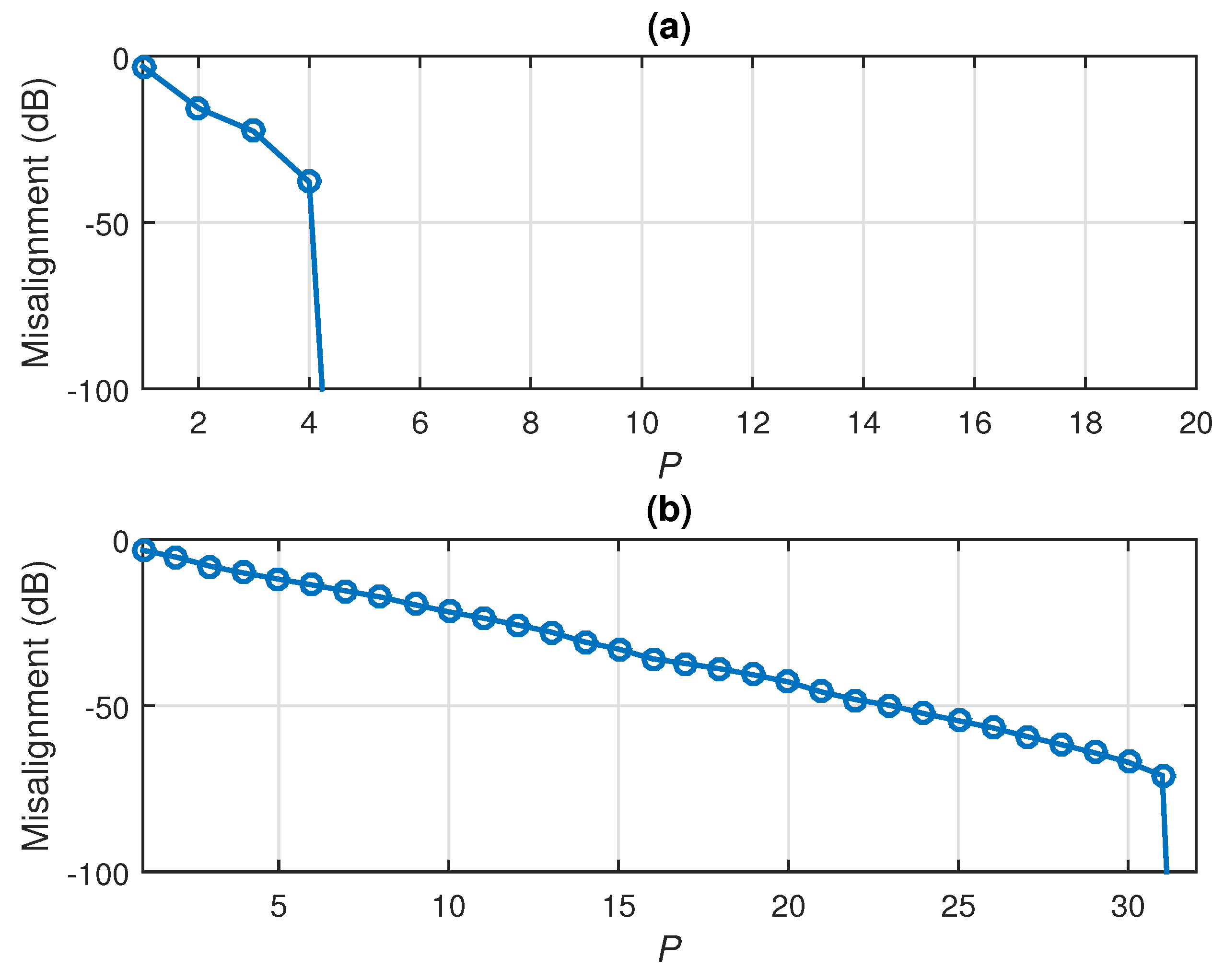
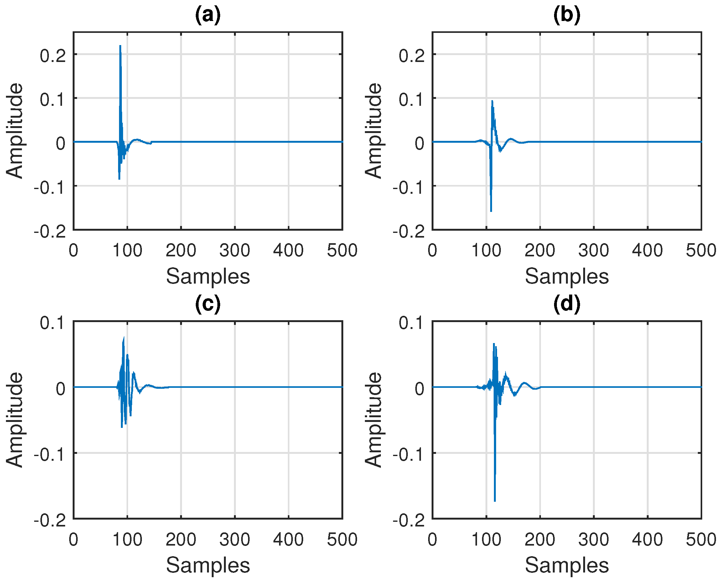
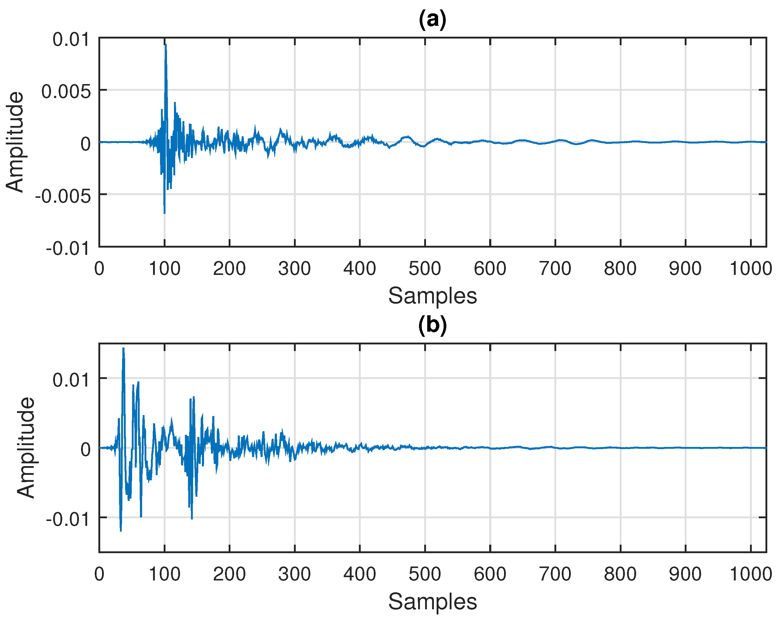
In order to show the validity of this approach, let us consider two scenarios that will also be detailed in the simulations provided in Section 6. In the first scenario, we consider $M=4$ impulse responses from the G168 Recommendation [63], which are network echo paths of length $L=500$, as depicted in Figure 3. In this case, the decomposition was performed using $L_1=25$ and $L_2=20$. In the second scenario, we used two acoustic impulse responses (i.e., $M=2$), each one having $L=1024$ coefficients, as depicted in Figure 4. 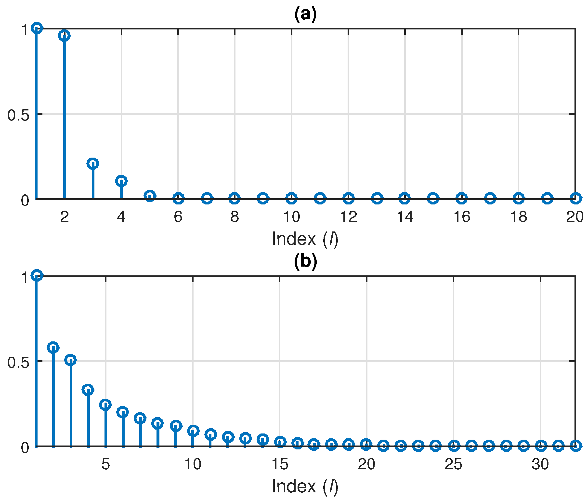Here, we set $L_1=L_2=32$ for the decomposition. In both cases, we evaluate the normalized misalignment from (55) and the evolution of the singular values ${\sigma }_l$ ($l=1,2,\dots ,L_2$) of the matrix ${\mathbf{H}}_{\mathrm{st}}$. As we can see in Figure 5, the normalized misalignment decreased with the value of P. This was much more apparent in the first scenario (corresponding to Figure 3), where the rank of ${\mathbf{H}}_{\mathrm{st}}$ resulted in $R=5$, as shown in Figure 5a. Consequently, a good approximation was obtained for $P\ll L_2$. In case of the acoustic impulse responses (i.e., the scenario from Figure 4), the resulting matrix ${\mathbf{H}}_{\mathrm{st}}$ was closer to being full rank, so that a larger value of P was required to obtain a good approximation. Nevertheless, as we can notice in Figure 5b, a value of P significantly lower as compared to $L_2$ led to reasonable attenuation of the misalignment (e.g., around $-20$ dB). This behavior is also supported in Figure 6, where we can notice the decreasing trend of the singular values (which are normalized to the maximum value).

5. Identification with the Wiener Filter

The identification of the LMISO system in (22) involves finding a real-valued filter, $\widehat{\underline{\mathbf{h}}}$, of length $ML$, which estimates the system $\underline{\mathbf{h}}$. The error signal can be defined as

$$\begin{array}{cc}\hfill e\left(k\right)& =d\left(k\right)-\widehat{y}\left(k\right),\hfill \end{array}$$

(56)

where $\widehat{y}\left(k\right)={\widehat{\underline{\mathbf{h}}}}^T\underline{\mathbf{x}}\left(k\right)$. The optimization criterion used to find the optimal filter is the mean-squared error (MSE):

$$\begin{array}{cc}\hfill \mathcal{J}\left(\widehat{\underline{\mathbf{h}}}\right)& =E\left[e^2\left(k\right)\right]\hfill \\ \hfill & ={\sigma }_d^2-2{\widehat{\underline{\mathbf{h}}}}^T\mathbf{p}+{\widehat{\underline{\mathbf{h}}}}^T\mathbf{R}\widehat{\underline{\mathbf{h}}},\hfill \end{array}$$

(57)

where $E[·]$ is the mathematical expectation, $\mathbf{p}=E\left[\underline{\mathbf{x}}\left(k\right)d\left(k\right)\right]$ represents the cross-correlation vector between $\underline{\mathbf{x}}\left(k\right)$ and $d\left(k\right)$, and $\mathbf{R}=E\left[\underline{\mathbf{x}}\left(k\right){\underline{\mathbf{x}}}^T\left(k\right)\right]$ denotes the covariance matrix of $\underline{\mathbf{x}}\left(k\right)$. After minimizing $\mathcal{J}\left(\widehat{\underline{\mathbf{h}}}\right)$, the celebrated (multichannel) Wiener filter is obtained:

$$\begin{array}{cc}\hfill {\widehat{\underline{\mathbf{h}}}}_{\mathrm{W}}& ={\mathbf{R}}^{-1}\mathbf{p}.\hfill \end{array}$$

(58)

Since the covariance matrix in the expression above is of size $ML\times ML$, a large number of data samples (more than $ML$) is needed in order to obtain a reliable solution.

An alternative approach to identifying the LMISO system in (22) and estimating $\underline{\mathbf{h}}$ as in the conventional case is to identify the LMISO system in (50) and estimate ${\mathbf{H}}_{\mathrm{st}}$. In the rest of this paper, the subscripts ${}_{\mathrm{st}}$ and ${}_{\mathrm{t}}$ are dropped in order to simplify the notation, and in this way ${\mathbf{H}}_{\mathrm{st}}={\sum }_{l=1}^{L_2}{\mathbf{h}}_{\mathrm{st}1,l}{\mathbf{h}}_{\mathrm{t}2,l}^T$ becomes $\mathbf{H}={\sum }_{l=1}^{L_2}{\mathbf{h}}_{1,l}{\mathbf{h}}_{2,l}^T$.

Next, we assume that $\mathrm{rank}\left(\mathbf{H}\right)=P\ll L_2$. Consequently, $\underline{\mathbf{h}}$ can be decomposed as

$$\begin{array}{cc}\hfill \underline{\mathbf{h}}& =\sum _{p=1}^P{\mathbf{h}}_{2,p}\otimes {\mathbf{h}}_{1,p},\hfill \end{array}$$

(59)

where the impulse responses ${\mathbf{h}}_{1,p}$ and ${\mathbf{h}}_{2,p}$ have lengths $M{L}_1$ and $L_2$, respectively. Therefore, the filter $\widehat{\underline{\mathbf{h}}}$ may also be decomposed as

$$\begin{array}{cc}\hfill \widehat{\underline{\mathbf{h}}}& =\sum _{p=1}^P{\widehat{\mathbf{h}}}_{2,p}\otimes {\widehat{\mathbf{h}}}_{1,p},\hfill \end{array}$$

(60)

where the filters ${\widehat{\mathbf{h}}}_{1,p}$ and ${\widehat{\mathbf{h}}}_{2,p}$ have lengths $M{L}_1$ and $L_2$, respectively. With the relations

$$\begin{array}{cc}\hfill {\widehat{\mathbf{h}}}_{2,p}\otimes {\widehat{\mathbf{h}}}_{1,p}& =\left({\widehat{\mathbf{h}}}_{2,p}\times 1\right)\otimes \left({\mathbf{I}}_{M{L}_1}\times {\widehat{\mathbf{h}}}_{1,p}\right)\hfill \\ \hfill & =\left({\widehat{\mathbf{h}}}_{2,p}\otimes {\mathbf{I}}_{M{L}_1}\right){\widehat{\mathbf{h}}}_{1,p}\hfill \end{array}$$

(61)

and

$$\begin{array}{cc}\hfill {\widehat{\mathbf{h}}}_{2,p}\otimes {\widehat{\mathbf{h}}}_{1,p}& =\left({\mathbf{I}}_{L_2}\times {\widehat{\mathbf{h}}}_{2,p}\right)\otimes \left({\widehat{\mathbf{h}}}_{1,p}\times 1\right)\hfill \\ \hfill & =\left({\mathbf{I}}_{L_2}\otimes {\widehat{\mathbf{h}}}_{1,p}\right){\widehat{\mathbf{h}}}_{2,p},\hfill \end{array}$$

(62)

where ${\mathbf{I}}_{M{L}_1}$ and ${\mathbf{I}}_{L_2}$ are the identity matrices of sizes $M{L}_1\times M{L}_1$ and $L_2\times L_2$, respectively, (60) may be rewritten as

$$\begin{array}{cc}\hfill \widehat{\underline{\mathbf{h}}}& =\sum _{p=1}^P{\widehat{\mathbf{H}}}_{2,p}{\widehat{\mathbf{h}}}_{1,p}\hfill \end{array}$$

(63)

$$\begin{array}{cc}\hfill & =\sum _{p=1}^P{\widehat{\mathbf{H}}}_{1,p}{\widehat{\mathbf{h}}}_{2,p},\hfill \end{array}$$

(64)

where

$$\begin{array}{cc}\hfill {\widehat{\mathbf{H}}}_{2,p}& ={\widehat{\mathbf{h}}}_{2,p}\otimes {\mathbf{I}}_{M{L}_1},\hfill \\ \hfill {\widehat{\mathbf{H}}}_{1,p}& ={\mathbf{I}}_{L_2}\otimes {\widehat{\mathbf{h}}}_{1,p}\hfill \end{array}$$

are matrices of sizes $ML\times M{L}_1$ and $ML\times L_2$, respectively. As a result, we may express the error signal defined in (56) in two distinct ways:

$$\begin{array}{cc}\hfill e\left(k\right)& =d\left(k\right)-\sum _{p=1}^P{\widehat{\mathbf{h}}}_{1,p}^T{\widehat{\mathbf{H}}}_{2,p}^T\underline{\mathbf{x}}\left(k\right)\hfill \\ \hfill & =d\left(k\right)-\sum _{p=1}^P{\widehat{\mathbf{h}}}_{1,p}^T{\mathbf{x}}_{2,p}\left(k\right)\hfill \\ \hfill & =d\left(k\right)-{\underline{\widehat{\mathbf{h}}}}_1^T{\underline{\mathbf{x}}}_2\left(k\right)\hfill \end{array}$$

(65)

and

$$\begin{array}{cc}\hfill e\left(k\right)& =d\left(k\right)-\sum _{p=1}^P{\widehat{\mathbf{h}}}_{2,p}^T{\widehat{\mathbf{H}}}_{1,p}^T\underline{\mathbf{x}}\left(k\right)\hfill \\ \hfill & =d\left(k\right)-\sum _{p=1}^P{\widehat{\mathbf{h}}}_{2,p}^T{\mathbf{x}}_{1,p}\left(k\right)\hfill \\ \hfill & =d\left(k\right)-{\underline{\widehat{\mathbf{h}}}}_2^T{\underline{\mathbf{x}}}_1\left(k\right),\hfill \end{array}$$

(66)

where

$$\begin{array}{cc}\hfill {\mathbf{x}}_{2,p}\left(k\right)& ={\widehat{\mathbf{H}}}_{2,p}^T\underline{\mathbf{x}}\left(k\right),\hfill \\ \hfill {\underline{\widehat{\mathbf{h}}}}_1& ={\left[\begin{array}{cccc}{\widehat{\mathbf{h}}}_{1,1}^T& {\widehat{\mathbf{h}}}_{1,2}^T& \cdots & {\widehat{\mathbf{h}}}_{1,P}^T\end{array}\right]}^T,\hfill \\ \hfill {\underline{\mathbf{x}}}_2\left(k\right)& ={\left[\begin{array}{cccc}{\mathbf{x}}_{2,1}^T\left(k\right)& {\mathbf{x}}_{2,2}^T\left(k\right)& \cdots & {\mathbf{x}}_{2,P}^T\left(k\right)\end{array}\right]}^T,\hfill \\ \hfill {\mathbf{x}}_{1,p}\left(k\right)& ={\widehat{\mathbf{H}}}_{1,p}^T\underline{\mathbf{x}}\left(k\right),\hfill \\ \hfill {\underline{\widehat{\mathbf{h}}}}_2& ={\left[\begin{array}{cccc}{\widehat{\mathbf{h}}}_{2,1}^T& {\widehat{\mathbf{h}}}_{2,2}^T& \cdots & {\widehat{\mathbf{h}}}_{2,P}^T\end{array}\right]}^T,\hfill \\ \hfill {\underline{\mathbf{x}}}_1\left(k\right)& ={\left[\begin{array}{cccc}{\mathbf{x}}_{1,1}^T\left(k\right)& {\mathbf{x}}_{1,2}^T\left(k\right)& \cdots & {\mathbf{x}}_{1,P}^T\left(k\right)\end{array}\right]}^T.\hfill \end{array}$$

Continuing with this formulation, we can write the MSE criterion as

$$\begin{array}{cc}\hfill \mathcal{J}\left({\underline{\widehat{\mathbf{h}}}}_1,{\underline{\widehat{\mathbf{h}}}}_2\right)& ={\sigma }_d^2-2{\underline{\widehat{\mathbf{h}}}}_1^T{\underline{\mathbf{p}}}_2+{\underline{\widehat{\mathbf{h}}}}_1^T{\underline{\mathbf{R}}}_2{\underline{\widehat{\mathbf{h}}}}_1\hfill \end{array}$$

(67)

$$\begin{array}{cc}\hfill & ={\sigma }_d^2-2{\underline{\widehat{\mathbf{h}}}}_2^T{\underline{\mathbf{p}}}_1+{\underline{\widehat{\mathbf{h}}}}_2^T{\underline{\mathbf{R}}}_1{\underline{\widehat{\mathbf{h}}}}_2,\hfill \end{array}$$

(68)

where

$$\begin{array}{cc}\hfill {\underline{\mathbf{p}}}_2& ={\left[\begin{array}{cccc}{\mathbf{p}}^T{\widehat{\mathbf{H}}}_{2,1}& {\mathbf{p}}^T{\widehat{\mathbf{H}}}_{2,2}& \cdots & {\mathbf{p}}^T{\widehat{\mathbf{H}}}_{2,P}\end{array}\right]}^T,\hfill \\ \hfill {\underline{\mathbf{R}}}_2& =\left[\begin{array}{cccc}{\widehat{\mathbf{H}}}_{2,1}^T\mathbf{R}{\widehat{\mathbf{H}}}_{2,1}& {\widehat{\mathbf{H}}}_{2,1}^T\mathbf{R}{\widehat{\mathbf{H}}}_{2,2}& \cdots & {\widehat{\mathbf{H}}}_{2,1}^T\mathbf{R}{\widehat{\mathbf{H}}}_{2,P}\\ {\widehat{\mathbf{H}}}_{2,2}^T\mathbf{R}{\widehat{\mathbf{H}}}_{2,1}& {\widehat{\mathbf{H}}}_{2,2}^T\mathbf{R}{\widehat{\mathbf{H}}}_{2,2}& \cdots & {\widehat{\mathbf{H}}}_{2,2}^T\mathbf{R}{\widehat{\mathbf{H}}}_{2,P}\\ ⋮& ⋮& \ddots & ⋮\\ {\widehat{\mathbf{H}}}_{2,P}^T\mathbf{R}{\widehat{\mathbf{H}}}_{2,1}& {\widehat{\mathbf{H}}}_{2,P}^T\mathbf{R}{\widehat{\mathbf{H}}}_{2,2}& \cdots & {\widehat{\mathbf{H}}}_{2,P}^T\mathbf{R}{\widehat{\mathbf{H}}}_{2,P}\end{array}\right],\hfill \\ \hfill {\underline{\mathbf{p}}}_1& ={\left[\begin{array}{cccc}{\mathbf{p}}^T{\widehat{\mathbf{H}}}_{1,1}& {\mathbf{p}}^T{\widehat{\mathbf{H}}}_{1,2}& \cdots & {\mathbf{p}}^T{\widehat{\mathbf{H}}}_{1,P}\end{array}\right]}^T,\hfill \\ \hfill {\underline{\mathbf{R}}}_1& =\left[\begin{array}{cccc}{\widehat{\mathbf{H}}}_{1,1}^T\mathbf{R}{\widehat{\mathbf{H}}}_{1,1}& {\widehat{\mathbf{H}}}_{1,1}^T\mathbf{R}{\widehat{\mathbf{H}}}_{1,2}& \cdots & {\widehat{\mathbf{H}}}_{1,1}^T\mathbf{R}{\widehat{\mathbf{H}}}_{1,P}\\ {\widehat{\mathbf{H}}}_{1,2}^T\mathbf{R}{\widehat{\mathbf{H}}}_{1,1}& {\widehat{\mathbf{H}}}_{1,2}^T\mathbf{R}{\widehat{\mathbf{H}}}_{1,2}& \cdots & {\widehat{\mathbf{H}}}_{1,2}^T\mathbf{R}{\widehat{\mathbf{H}}}_{1,P}\\ ⋮& ⋮& \ddots & ⋮\\ {\widehat{\mathbf{H}}}_{1,P}^T\mathbf{R}{\widehat{\mathbf{H}}}_{1,1}& {\widehat{\mathbf{H}}}_{1,P}^T\mathbf{R}{\widehat{\mathbf{H}}}_{1,2}& \cdots & {\widehat{\mathbf{H}}}_{1,P}^T\mathbf{R}{\widehat{\mathbf{H}}}_{1,P}\end{array}\right].\hfill \end{array}$$

It can be noticed that the matrices ${\underline{\mathbf{R}}}_1$ and ${\underline{\mathbf{R}}}_2$ have sizes $P{L}_2\times P{L}_2$ and $PM{L}_1\times PM{L}_1$, respectively, which can be much smaller than the size of $\mathbf{R}$, which is $ML\times ML$. Additionally, at least $PM{L}_1$ data samples are required for the estimation of the statistics in the MSE from (67) or (68), whereas in order to estimate the statistics in the conventional MSE from (57), we need at least $ML$ data samples. When ${\underline{\widehat{\mathbf{h}}}}_2$ is fixed, we can express (67) as

$$\begin{array}{cc}\hfill {\mathcal{J}}_{{\underline{\widehat{\mathbf{h}}}}_2}\left({\underline{\widehat{\mathbf{h}}}}_1\right)& ={\sigma }_d^2-2{\underline{\widehat{\mathbf{h}}}}_1^T{\underline{\mathbf{p}}}_2+{\underline{\widehat{\mathbf{h}}}}_1^T{\underline{\mathbf{R}}}_2{\underline{\widehat{\mathbf{h}}}}_1\hfill \end{array}$$

(69)

and when ${\underline{\widehat{\mathbf{h}}}}_1$ is fixed, we can write (68) as

$$\begin{array}{cc}\hfill {\mathcal{J}}_{{\underline{\widehat{\mathbf{h}}}}_1}\left({\underline{\widehat{\mathbf{h}}}}_2\right)& ={\sigma }_d^2-2{\underline{\widehat{\mathbf{h}}}}_2^T{\underline{\mathbf{p}}}_1+{\underline{\widehat{\mathbf{h}}}}_2^T{\underline{\mathbf{R}}}_1{\underline{\widehat{\mathbf{h}}}}_2.\hfill \end{array}$$

(70)

This represents a bilinear optimization strategy [64].

In order to obtain the optimal filters, an iterative algorithm similar to the those presented in [24,43] can be derived. At iteration 0, we may take

$$\begin{array}{cc}\hfill {\widehat{\mathbf{h}}}_{2,p}^{\left(0\right)}& ={\left[\begin{array}{cccc}ϵ& 0& \cdots & 0\end{array}\right]}^T,p=1,2,\dots ,P,\hfill \end{array}$$

where $0<ϵ\le 1$. Then, we may form ${\widehat{\mathbf{H}}}_{2,p}^{\left(0\right)}={\widehat{\mathbf{h}}}_{2,p}^{\left(0\right)}\otimes {\mathbf{I}}_{M{L}_1}$ and

$$\begin{array}{cc}\hfill {\underline{\mathbf{p}}}_2^{\left(0\right)}& ={\left[\begin{array}{cccc}{\mathbf{p}}^T{\widehat{\mathbf{H}}}_{2,1}^{\left(0\right)}& {\mathbf{p}}^T{\widehat{\mathbf{H}}}_{2,2}^{\left(0\right)}& \cdots & {\mathbf{p}}^T{\widehat{\mathbf{H}}}_{2,P}^{\left(0\right)}\end{array}\right]}^T,\hfill \\ \hfill {\underline{\mathbf{R}}}_2^{\left(0\right)}& =\left[\begin{array}{cccc}{\left({\widehat{\mathbf{H}}}_{2,1}^{\left(0\right)}\right)}^T\mathbf{R}{\widehat{\mathbf{H}}}_{2,1}^{\left(0\right)}& {\left({\widehat{\mathbf{H}}}_{2,1}^{\left(0\right)}\right)}^T\mathbf{R}{\widehat{\mathbf{H}}}_{2,2}^{\left(0\right)}& \cdots & {\left({\widehat{\mathbf{H}}}_{2,1}^{\left(0\right)}\right)}^T\mathbf{R}{\widehat{\mathbf{H}}}_{2,P}^{\left(0\right)}\\ {\left({\widehat{\mathbf{H}}}_{2,2}^{\left(0\right)}\right)}^T\mathbf{R}{\widehat{\mathbf{H}}}_{2,1}^{\left(0\right)}& {\left({\widehat{\mathbf{H}}}_{2,2}^{\left(0\right)}\right)}^T\mathbf{R}{\widehat{\mathbf{H}}}_{2,2}^{\left(0\right)}& \cdots & {\left({\widehat{\mathbf{H}}}_{2,2}^{\left(0\right)}\right)}^T\mathbf{R}{\widehat{\mathbf{H}}}_{2,P}^{\left(0\right)}\\ ⋮& ⋮& \ddots & ⋮\\ {\left({\widehat{\mathbf{H}}}_{2,P}^{\left(0\right)}\right)}^T\mathbf{R}{\widehat{\mathbf{H}}}_{2,1}^{\left(0\right)}& {\left({\widehat{\mathbf{H}}}_{2,P}^{\left(0\right)}\right)}^T\mathbf{R}{\widehat{\mathbf{H}}}_{2,2}^{\left(0\right)}& \cdots & {\left({\widehat{\mathbf{H}}}_{2,P}^{\left(0\right)}\right)}^T\mathbf{R}{\widehat{\mathbf{H}}}_{2,P}^{\left(0\right)}\end{array}\right].\hfill \end{array}$$

By substituting the quantities above into the MSE from (69), we get at iteration 1:

$$\begin{array}{cc}\hfill {\mathcal{J}}_{{\underline{\widehat{\mathbf{h}}}}_2}\left({\underline{\widehat{\mathbf{h}}}}_1^{\left(1\right)}\right)& ={\sigma }_d^2-2{\left({\underline{\widehat{\mathbf{h}}}}_1^{\left(1\right)}\right)}^T{\underline{\mathbf{p}}}_2^{\left(0\right)}+{\left({\underline{\widehat{\mathbf{h}}}}_1^{\left(1\right)}\right)}^T{\underline{\mathbf{R}}}_2^{\left(0\right)}{\underline{\widehat{\mathbf{h}}}}_1^{\left(1\right)},\hfill \end{array}$$

(71)

which can be minimized with respect to ${\underline{\widehat{\mathbf{h}}}}_1^{\left(1\right)}$, thereby yielding

$$\begin{array}{cc}\hfill {\underline{\widehat{\mathbf{h}}}}_1^{\left(1\right)}& ={\left({\underline{\mathbf{R}}}_2^{\left(0\right)}\right)}^{-1}{\underline{\mathbf{p}}}_2^{\left(0\right)}.\hfill \end{array}$$

(72)

Next, using ${\underline{\widehat{\mathbf{h}}}}_1^{\left(1\right)}$, we can construct ${\widehat{\mathbf{H}}}_{1,p}^{\left(1\right)}={\mathbf{I}}_{L_2}\otimes {\widehat{\mathbf{h}}}_{1,p}^{\left(1\right)}$ and

$$\begin{array}{cc}\hfill {\underline{\mathbf{p}}}_1^{\left(1\right)}& ={\left[\begin{array}{cccc}{\mathbf{p}}^T{\widehat{\mathbf{H}}}_{1,1}^{\left(1\right)}& {\mathbf{p}}^T{\widehat{\mathbf{H}}}_{1,2}^{\left(1\right)}& \cdots & {\mathbf{p}}^T{\widehat{\mathbf{H}}}_{1,P}^{\left(1\right)}\end{array}\right]}^T,\hfill \\ \hfill {\underline{\mathbf{R}}}_1^{\left(1\right)}& =\left[\begin{array}{cccc}{\left({\widehat{\mathbf{H}}}_{1,1}^{\left(1\right)}\right)}^T\mathbf{R}{\widehat{\mathbf{H}}}_{1,1}^{\left(1\right)}& {\left({\widehat{\mathbf{H}}}_{1,1}^{\left(1\right)}\right)}^T\mathbf{R}{\widehat{\mathbf{H}}}_{1,2}^{\left(1\right)}& \cdots & {\left({\widehat{\mathbf{H}}}_{1,1}^{\left(1\right)}\right)}^T\mathbf{R}{\widehat{\mathbf{H}}}_{1,P}^{\left(1\right)}\\ {\left({\widehat{\mathbf{H}}}_{1,2}^{\left(1\right)}\right)}^T\mathbf{R}{\widehat{\mathbf{H}}}_{1,1}^{\left(1\right)}& {\left({\widehat{\mathbf{H}}}_{1,2}^{\left(1\right)}\right)}^T\mathbf{R}{\widehat{\mathbf{H}}}_{1,2}^{\left(1\right)}& \cdots & {\left({\widehat{\mathbf{H}}}_{1,2}^{\left(1\right)}\right)}^T\mathbf{R}{\widehat{\mathbf{H}}}_{1,P}^{\left(1\right)}\\ ⋮& ⋮& \ddots & ⋮\\ {\left({\widehat{\mathbf{H}}}_{1,P}^{\left(1\right)}\right)}^T\mathbf{R}{\widehat{\mathbf{H}}}_{1,1}^{\left(1\right)}& {\left({\widehat{\mathbf{H}}}_{1,P}^{\left(1\right)}\right)}^T\mathbf{R}{\widehat{\mathbf{H}}}_{1,2}^{\left(1\right)}& \cdots & {\left({\widehat{\mathbf{H}}}_{1,P}^{\left(1\right)}\right)}^T\mathbf{R}{\widehat{\mathbf{H}}}_{1,P}^{\left(1\right)}\end{array}\right].\hfill \end{array}$$

Consequently, the MSE from (70) is

$$\begin{array}{cc}\hfill {\mathcal{J}}_{{\underline{\widehat{\mathbf{h}}}}_1}\left({\underline{\widehat{\mathbf{h}}}}_2^{\left(1\right)}\right)& ={\sigma }_d^2-2{\left({\underline{\widehat{\mathbf{h}}}}_2^{\left(1\right)}\right)}^T{\underline{\mathbf{p}}}_1^{\left(1\right)}+{\left({\underline{\widehat{\mathbf{h}}}}_2^{\left(1\right)}\right)}^T{\underline{\mathbf{R}}}_1^{\left(1\right)}{\underline{\widehat{\mathbf{h}}}}_2^{\left(1\right)}.\hfill \end{array}$$

(73)

The minimization of the previous expression with respect to ${\underline{\widehat{\mathbf{h}}}}_2^{\left(1\right)}$ gives

$$\begin{array}{cc}\hfill {\underline{\widehat{\mathbf{h}}}}_2^{\left(1\right)}& ={\left({\underline{\mathbf{R}}}_1^{\left(1\right)}\right)}^{-1}{\underline{\mathbf{p}}}_1^{\left(1\right)}.\hfill \end{array}$$

(74)

By iterating further, we obtain at iteration n

$$\begin{array}{cc}\hfill {\underline{\widehat{\mathbf{h}}}}_1^{\left(n\right)}& ={\left({\underline{\mathbf{R}}}_2^{(n-1)}\right)}^{-1}{\underline{\mathbf{p}}}_2^{(n-1)},\hfill \end{array}$$

(75)

$$\begin{array}{cc}\hfill {\underline{\widehat{\mathbf{h}}}}_2^{\left(n\right)}& ={\left({\underline{\mathbf{R}}}_1^{\left(n\right)}\right)}^{-1}{\underline{\mathbf{p}}}_1^{\left(n\right)},\hfill \end{array}$$

(76)

where ${\underline{\mathbf{R}}}_2^{(n-1)}$, ${\underline{\mathbf{p}}}_2^{(n-1)}$, ${\underline{\mathbf{R}}}_1^{\left(n\right)}$, and ${\underline{\mathbf{p}}}_1^{\left(n\right)}$ are constructed similarly to ${\underline{\mathbf{R}}}_2^{\left(0\right)}$, ${\underline{\mathbf{p}}}_2^{\left(0\right)}$, ${\underline{\mathbf{R}}}_1^{\left(1\right)}$, and ${\underline{\mathbf{p}}}_1^{\left(1\right)}$, respectively. In the end, the Wiener filter at iteration n results as

$$\begin{array}{cc}\hfill {\widehat{\underline{\mathbf{h}}}}_{\mathrm{W}}^{\left(n\right)}& =\sum _{p=1}^P{\widehat{\mathbf{h}}}_{2,p}^{\left(n\right)}\otimes {\widehat{\mathbf{h}}}_{1,p}^{\left(n\right)}.\hfill \end{array}$$

(77)

The multichannel iterative Wiener filter is summarized in

Table 1. The multichannel iterative Wiener filter.

$$\begin{array}{ccc}& & \underline{\mathrm{Data}:}\mathbf{R},\mathbf{p}\left(\mathrm{estimated}\mathrm{statistics}\mathrm{based}\mathrm{on}N\mathrm{data}\mathrm{samples}\right),\hfill \\ & & P\left(\mathrm{decomposition}\mathrm{parameter}\right),\delta >0\left(\mathrm{regularization}\mathrm{constant}\right)\hfill \\ & & \underline{\mathrm{Initialization}:}\hfill \\ & & \mathrm{Provide}\mathrm{the}\mathrm{initial}\mathrm{coefficients}\mathrm{of}\mathrm{the}\mathrm{filter}{\widehat{\mathbf{h}}}_{2,p}^{\left(0\right)}(\mathrm{for}p=1,2,\dots ,P):\hfill \\ & & {\widehat{\mathbf{h}}}_{2,p}^{\left(0\right)}={\left[\begin{array}{cccc}ϵ& 0& \cdots & 0\end{array}\right]}^T,p=1,2,\dots ,P(0<ϵ\le 1)\hfill \\ & & \mathrm{Compute}\mathrm{the}\mathrm{initial}\mathrm{statistics}{\underline{\mathbf{p}}}_2^{\left(0\right)}\mathrm{and}{\underline{\mathbf{R}}}_2^{\left(0\right)}:\hfill \\ & & {\widehat{\mathbf{H}}}_{2,\mathbf{p}}^{\left(0\right)}={\widehat{\mathbf{h}}}_{2,p}^{\left(0\right)}\otimes {\mathbf{I}}_{M{L}_1},p=1,2,\dots ,P\hfill \\ & & {\underline{\mathbf{p}}}_2^{\left(0\right)}={\left[\begin{array}{ccc}{\mathbf{p}}^T{\widehat{\mathbf{H}}}_{2,1}^{\left(0\right)}& \cdots & {\mathbf{p}}^T{\widehat{\mathbf{H}}}_{2,P}^{\left(0\right)}\end{array}\right]}^T\hfill \\ & & {\underline{\mathbf{R}}}_2^{\left(0\right)}=\left[\begin{array}{ccc}{\left({\widehat{\mathbf{H}}}_{2,1}^{\left(0\right)}\right)}^T\mathbf{R}{\widehat{\mathbf{H}}}_{2,1}^{\left(0\right)}& \cdots & {\left({\widehat{\mathbf{H}}}_{2,1}^{\left(0\right)}\right)}^T\mathbf{R}{\widehat{\mathbf{H}}}_{2,P}^{\left(0\right)}\\ ⋮& \ddots & ⋮\\ {\left({\widehat{\mathbf{H}}}_{2,P}^{\left(0\right)}\right)}^T\mathbf{R}{\widehat{\mathbf{H}}}_{2,1}^{\left(0\right)}& \cdots & {\left({\widehat{\mathbf{H}}}_{2,P}^{\left(0\right)}\right)}^T\mathbf{R}{\widehat{\mathbf{H}}}_{2,P}^{\left(0\right)}\end{array}\right]\hfill \\ & & \underline{\mathrm{For}}n=1,2,\mathbf{\dots }:\hfill \\ & & \mathrm{Compute}\mathrm{the}\mathrm{coefficients}\mathrm{of}\mathrm{the}\mathrm{filter}{\underline{\widehat{\mathbf{h}}}}_1^{\left(n\right)}\mathrm{based}\mathrm{on}\left(75\right):\hfill \\ & & {\underline{\widehat{\mathbf{h}}}}_1^{\left(n\right)}={\left({\underline{\mathbf{R}}}_2^{(n-1)}+\delta {\mathbf{I}}_{PM{L}_1}\right)}^{-1}{\underline{\mathbf{p}}}_2^{(n-1)}={\left[\begin{array}{ccc}{\left({\widehat{\mathbf{h}}}_{1,1}^{\left(n\right)}\right)}^T& \cdots & {\left({\widehat{\mathbf{h}}}_{1,P}^{\left(n\right)}\right)}^T\end{array}\right]}^T\hfill \\ & & \mathrm{Compute}\mathrm{the}\mathrm{statistics}{\underline{\mathbf{p}}}_1^{\left(n\right)}\mathrm{and}{\underline{\mathbf{R}}}_1^{\left(n\right)}:\hfill \\ & & {\widehat{\mathbf{H}}}_{1,p}^{\left(n\right)}={\mathbf{I}}_{L_2}\otimes {\widehat{\mathbf{h}}}_{1,p}^{\left(n\right)},p=1,2,\dots ,P\hfill \\ & & {\underline{\mathbf{p}}}_1^{\left(n\right)}={\left[\begin{array}{ccc}{\mathbf{p}}^T{\widehat{\mathbf{H}}}_{1,1}^{\left(n\right)}& \cdots & {\mathbf{p}}^T{\widehat{\mathbf{H}}}_{1,P}^{\left(n\right)}\end{array}\right]}^T\hfill \\ & & {\underline{\mathbf{R}}}_1^{\left(n\right)}=\left[\begin{array}{ccc}{\left({\widehat{\mathbf{H}}}_{1,1}^{\left(n\right)}\right)}^T\mathbf{R}{\widehat{\mathbf{H}}}_{1,1}^{\left(n\right)}& \cdots & {\left({\widehat{\mathbf{H}}}_{1,1}^{\left(1\right)}\right)}^T\mathbf{R}{\widehat{\mathbf{H}}}_{1,P}^{\left(1\right)}\\ ⋮& \ddots & ⋮\\ {\left({\widehat{\mathbf{H}}}_{1,P}^{\left(n\right)}\right)}^T\mathbf{R}{\widehat{\mathbf{H}}}_{1,1}^{\left(n\right)}& \cdots & {\left({\widehat{\mathbf{H}}}_{1,P}^{\left(n\right)}\right)}^T\mathbf{R}{\widehat{\mathbf{H}}}_{1,P}^{\left(n\right)}\end{array}\right]\hfill \\ & & \mathrm{Compute}\mathrm{the}\mathrm{coefficients}\mathrm{of}\mathrm{the}\mathrm{filter}{\underline{\widehat{\mathbf{h}}}}_2^{\left(n\right)}\mathrm{based}\mathrm{on}\left(76\right):\hfill \\ & & {\underline{\widehat{\mathbf{h}}}}_2^{\left(n\right)}={\left({\underline{\mathbf{R}}}_1^{\left(n\right)}+\delta {\mathbf{I}}_{P{L}_2}\right)}^{-1}{\underline{\mathbf{p}}}_1^{\left(n\right)}={\left[\begin{array}{ccc}{\left({\widehat{\mathbf{h}}}_{2,1}^{\left(n\right)}\right)}^T& \cdots & {\left({\widehat{\mathbf{h}}}_{2,P}^{\left(n\right)}\right)}^T\end{array}\right]}^T\hfill \\ & & \mathrm{Compute}\mathrm{the}\mathrm{statistics}{\underline{\mathbf{p}}}_2^{\left(n\right)}\mathrm{and}{\underline{\mathbf{R}}}_2^{\left(n\right)}:\hfill \\ & & {\widehat{\mathbf{H}}}_{2,p}^{\left(n\right)}={\widehat{\mathbf{h}}}_{2,p}^{\left(n\right)}\otimes {\mathbf{I}}_{M{L}_1},p=1,2,\dots ,P\hfill \\ & & {\underline{\mathbf{p}}}_2^{\left(n\right)}={\left[\begin{array}{ccc}{\mathbf{p}}^T{\widehat{\mathbf{H}}}_{2,1}^{\left(n\right)}& \cdots & {\mathbf{p}}^T{\widehat{\mathbf{H}}}_{2,P}^{\left(n\right)}\end{array}\right]}^T\hfill \\ & & {\underline{\mathbf{R}}}_2^{\left(n\right)}=\left[\begin{array}{ccc}{\left({\widehat{\mathbf{H}}}_{2,1}^{\left(n\right)}\right)}^T\mathbf{R}{\widehat{\mathbf{H}}}_{2,1}^{\left(n\right)}& \cdots & {\left({\widehat{\mathbf{H}}}_{2,1}^{\left(n\right)}\right)}^T\mathbf{R}{\widehat{\mathbf{H}}}_{2,P}^{\left(n\right)}\\ ⋮& \ddots & ⋮\\ {\left({\widehat{\mathbf{H}}}_{2,P}^{\left(n\right)}\right)}^T\mathbf{R}{\widehat{\mathbf{H}}}_{2,1}^{\left(n\right)}& \cdots & {\left({\widehat{\mathbf{H}}}_{2,P}^{\left(n\right)}\right)}^T\mathbf{R}{\widehat{\mathbf{H}}}_{2,P}^{\left(n\right)}\end{array}\right]\hfill \\ & & \mathrm{Compute}\mathrm{the}\mathrm{coefficients}\mathrm{of}\mathrm{the}\mathrm{Wiener}\mathrm{filter}{\underline{\widehat{\mathbf{h}}}}_W^{\left(n\right)}\mathrm{based}\mathrm{on}\left(77\right):\hfill \\ & & {\underline{\widehat{\mathbf{h}}}}_{\mathrm{W}}^{\left(n\right)}=\sum _{p=1}^P{\widehat{\mathbf{h}}}_{2,p}^{\left(n\right)}\otimes {\widehat{\mathbf{h}}}_{1,p}^{\left(n\right)}\hfill \\ \hfill \end{array}$$

. For $M=1$ (i.e., single-channel case), the problem is reduced to a regular SISO scenario, and the algorithm becomes equivalent to the version developed in [43]. Additionally, if the system is perfectly separable/decomposable, we can obtain the optimal solution for $P=1$. In this case, the iterative Wiener filter for bilinear forms (proposed in [24]) is obtained.

6. Simulation Results

In this section, we evaluate the performance of the conventional and iterative Wiener filters in two different scenarios. The first one is dedicated to the case of independent input signals, ${\mathbf{x}}_m\left(k\right),m=1,2,\dots ,M$. The second scenario is more challenging, since it considers the case when the input signals are coming from the same source and they are linearly related. In both cases, the performance measure used to evaluate the overall behavior is the normalized misalignment (in dB), which is related to the spatiotemporal impulse response of the system, $\underline{\mathbf{h}}$. In this framework, the solution provided by the conventional Wiener filter is given in (58), so that the performance measure is evaluated as

$$\begin{array}{cc}\hfill \mathcal{M}\left(\underline{\mathbf{h}},{\widehat{\underline{\mathbf{h}}}}_{\mathrm{W}}\right)& =20{\log }_{10}\frac{{∥\underline{\mathbf{h}}-{\widehat{\underline{\mathbf{h}}}}_{\mathrm{W}}∥}_2}{{∥\underline{\mathbf{h}}∥}_2}.\hfill \end{array}$$

(78)

Similarly, for the iterative Wiener filter from (77), the performance measure results in

$$\begin{array}{cc}\hfill \mathcal{M}\left(\underline{\mathbf{h}},{\widehat{\underline{\mathbf{h}}}}_{\mathrm{W}}^{\left(n\right)}\right)& =20{\log }_{10}\frac{{∥\underline{\mathbf{h}}-{\widehat{\underline{\mathbf{h}}}}_{\mathrm{W}}^{\left(n\right)}∥}_2}{{∥\underline{\mathbf{h}}∥}_2}.\hfill \end{array}$$

(79)

Both the conventional and iterative Wiener filters rely on the estimation of the statistics, i.e., the covariance matrix $\mathbf{R}$ and the cross-correlation vector $\mathbf{p}$. Considering that N data samples are available, these estimates result in

$$\begin{array}{cc}\hfill \widehat{\mathbf{R}}& =\frac{1}{N}\sum _{k=1}^N\underline{\mathbf{x}}\left(k\right){\underline{\mathbf{x}}}^T\left(k\right),\hfill \end{array}$$

(80)

$$\begin{array}{cc}\hfill \widehat{\mathbf{p}}& =\frac{1}{N}\sum _{k=1}^N\underline{\mathbf{x}}\left(k\right)d\left(k\right).\hfill \end{array}$$

(81)

Clearly, the value of N influences the quality of these estimates. Nevertheless, in practice, only a small amount of data could be available, which makes the identification process more challenging. In this case, the advantages of the iterative Wiener filter (which operates with smaller data structures) become more apparent, as will be supported in the following analysis.

The additive noise may also affect the accuracy of the Wiener solution. In relation to (13) or (22), the signal-to-noise ratio (SNR) can be defined as

$$\begin{array}{cc}\hfill \mathrm{SNR}& =\frac{{\sigma }_y^2}{{\sigma }_w^2},\hfill \end{array}$$

(82)

where ${\sigma }_y^2$ and ${\sigma }_w^2$ are the variances of the output signal and noise, respectively. In practice, the Wiener solution is satisfactory with reasonable levels of the SNR, but it is not with small values of the SNR. In our experiments, different values of the SNR were used, in order to illustrate this behavior.

All the experiments were performed using MATLAB R2018b on an Asus GL552VX device (Windows 10 OS), having an Intel Core i7-6700HQ CPU @ 2.60 GHz, with four cores, eight logical processors, and 16 GB of RAM. In the first set of experiments, we considered the case of M independent input signals, which were generated as AR(1) processes. These were obtained by filtering white Gaussian noise through an AR(1) model with a pole at 0.9. Of course, different other inputs can be used instead of the AR(1) model. The most common considerations are: (i) the input signal $x\left(k\right)$ is wide-sense stationary, (ii) all of the signals (i.e., $x\left(k\right)$, $d\left(k\right)$, and $w\left(k\right)$) have zero means, and (iii) usually, the noise $w\left(k\right)$ is not correlated with the input signal $x\left(k\right)$.

In our scenario, the number of channels was $M=4$ and their impulse responses were chosen from the G168 Recommendation [63]. They were network echo paths of length $L=500$, as depicted in Figure 3.

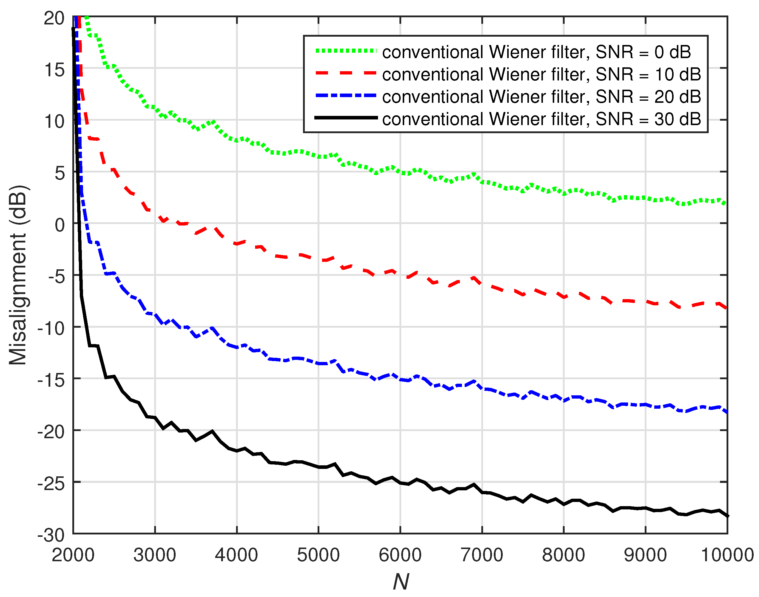
As mentioned before, the performance of the Wiener solution is influenced by the value of N and the level of the SNR. This is supported in Figure 7, where the performance of the conventional Wiener filter from (58) is illustrated for different values of N (from 2000 to 10,000 available data samples) and SNR levels (from 0 dB to 30 dB). As we can notice, a larger value of N (i.e., $N\gg ML$) is required to obtain reasonable attenuation of the misalignment. Additionally, as expected, a more accurate solution was obtained with higher SNRs.

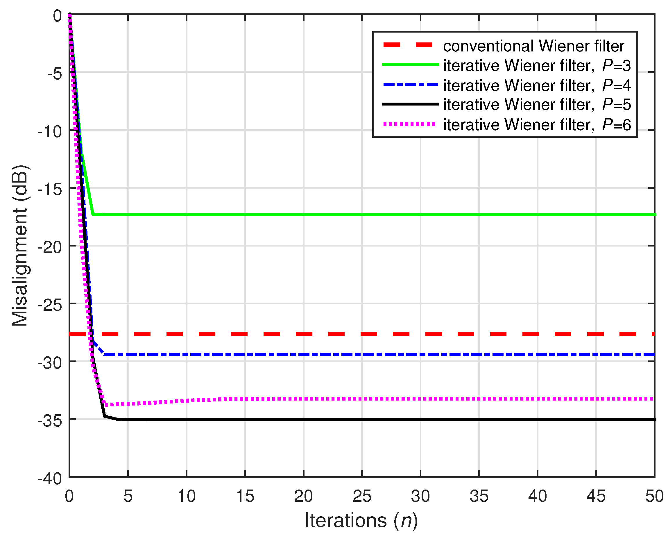
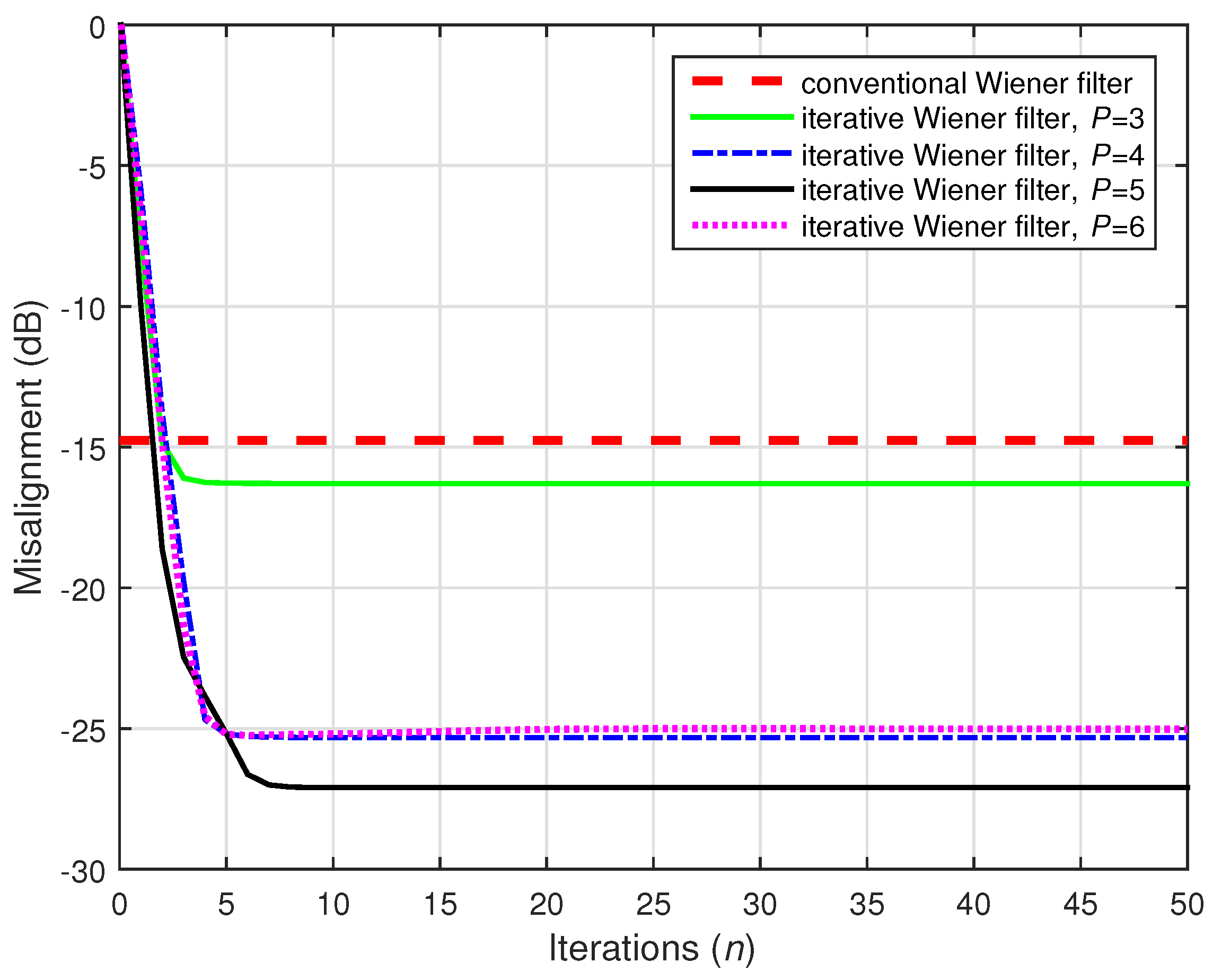
In this context, let us first compare the performance of the conventional and iterative Wiener filters in “favorable” conditions, using a large amount of data to estimate the statistics (i.e., $N=$ 10,000), in a high SNR environment (i.e., $\mathrm{SNR}=30$ dB). The iterative Wiener filter from (77) uses $L_1=25$, $L_2=20$, and different values of the decomposition parameter P (from 3 to 6). These values are much lower than $L_2$, which represents an important advantage, as discussed in Section 5. We should also note that for the scenario considered in this first set of experiments (using the setup from Figure 3), the rank of the matrix $\mathbf{H}$ (or ${\mathbf{H}}_{\mathrm{st}}$) was equal to $R=5$. As we can notice in Figure 8, the iterative Wiener filter was able to outperform the conventional Wiener filter for most of the values of P. Even the case of $P=3<R\ll L_2$ led to reasonable attenuation of the misalignment. Moreover, all these iterative solutions were obtained in only a few iterations.

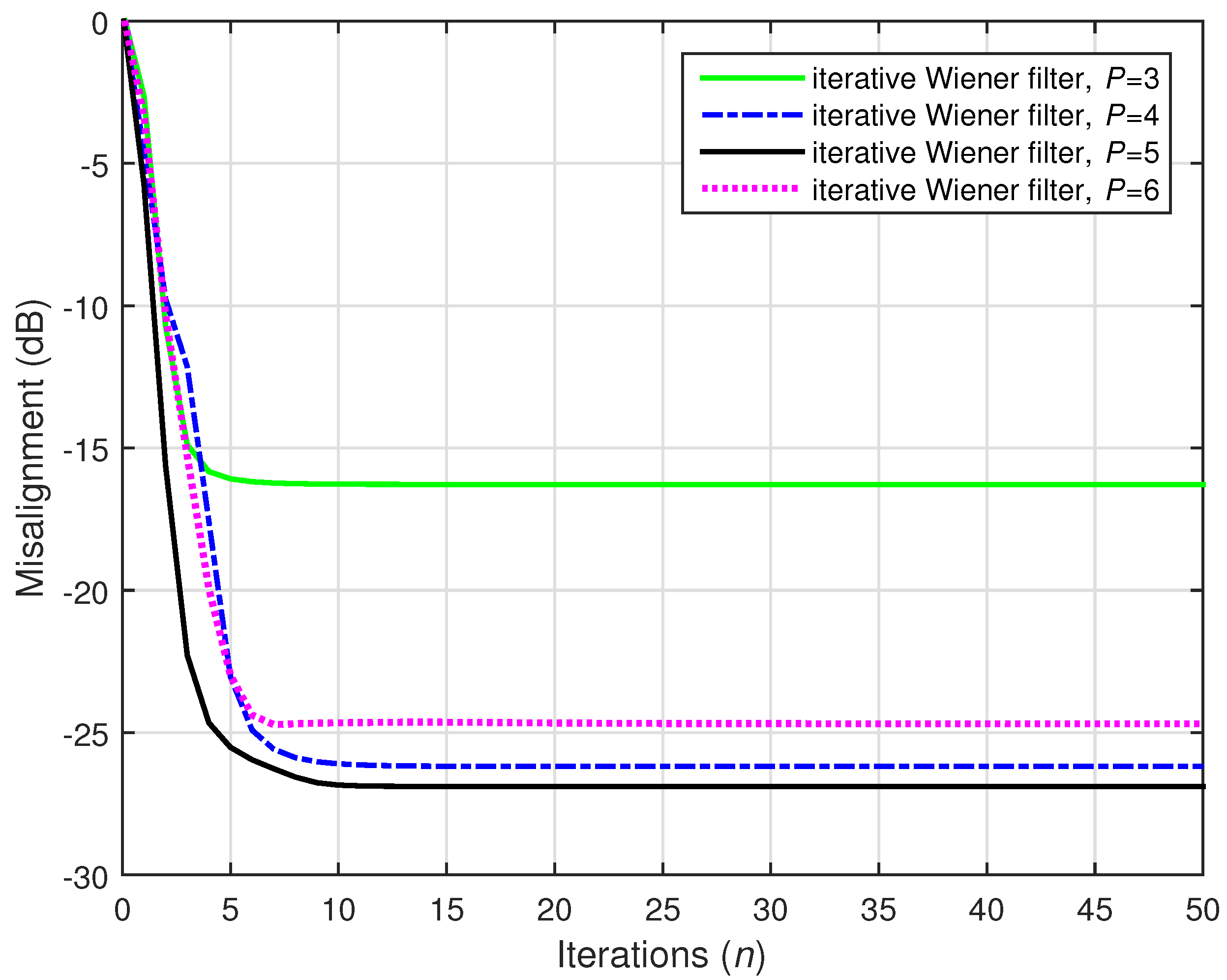
The advantages of the iterative Wiener filter became more apparent when less data were available to estimate the statistics. The previous simulation was repeated, but using $N=2500$ (Figure 9). According to the results shown in Figure 7, the performance of the conventional Wiener filter was affected in this case (even for $\mathrm{SNR}=30$ dB); its misalignment level was close to $-15$ dB. This result is also confirmed in Figure 9. Most importantly, the iterative Wiener filter outperformed the conventional solution for all the values of P, thereby being more robust in this case due to the low-dimensional data structures used in its development.

For the scenario considered in this first set of experiments, the length of the spatiotemporal impulse response was $ML=4\times 500=2000$. Therefore, the case $N=2000$ represents a limit in terms of the available amount of data. As we can notice in Figure 7, the conventional Wiener filter could not cope with this limit. On the other hand, the iterative Wiener filter was still able to obtain good performances, for $P\ll L_2$, as supported in Figure 10.

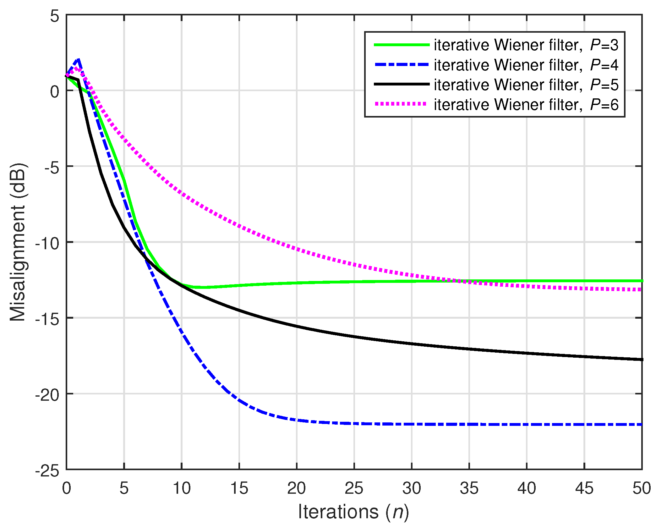
Furthermore, using $N<ML$ is a significant challenge in terms of system identification, since apparently we deal with an "incomplete" scenario, when trying to estimate $ML$ coefficients using less data. Clearly, the conventional Wiener filter cannot be used in this case. However, the iterative Wiener filter reformulates the original system identification problem (of size $ML$) as a combination of low-dimension solutions of size $PM{L}_1$ and $P{L}_2$, with $P\ll L_2$. Hence, it could overcome this limit of $N<ML$. This is supported in Figure 11: only $N=1000$ data samples were available for the estimation of the statistics. Even in this challenging case, the iterative Wiener filter was able to provide a good attenuation of the misalignment, in a relatively small number of iterations. This represents an important feature and a significant advantage when dealing with small amounts of data. In other words, the iterative Wiener filter exploiting the decomposition-based approach can be used to solve system identification problems with highly incomplete information, which is a condition imposed in many important applications.

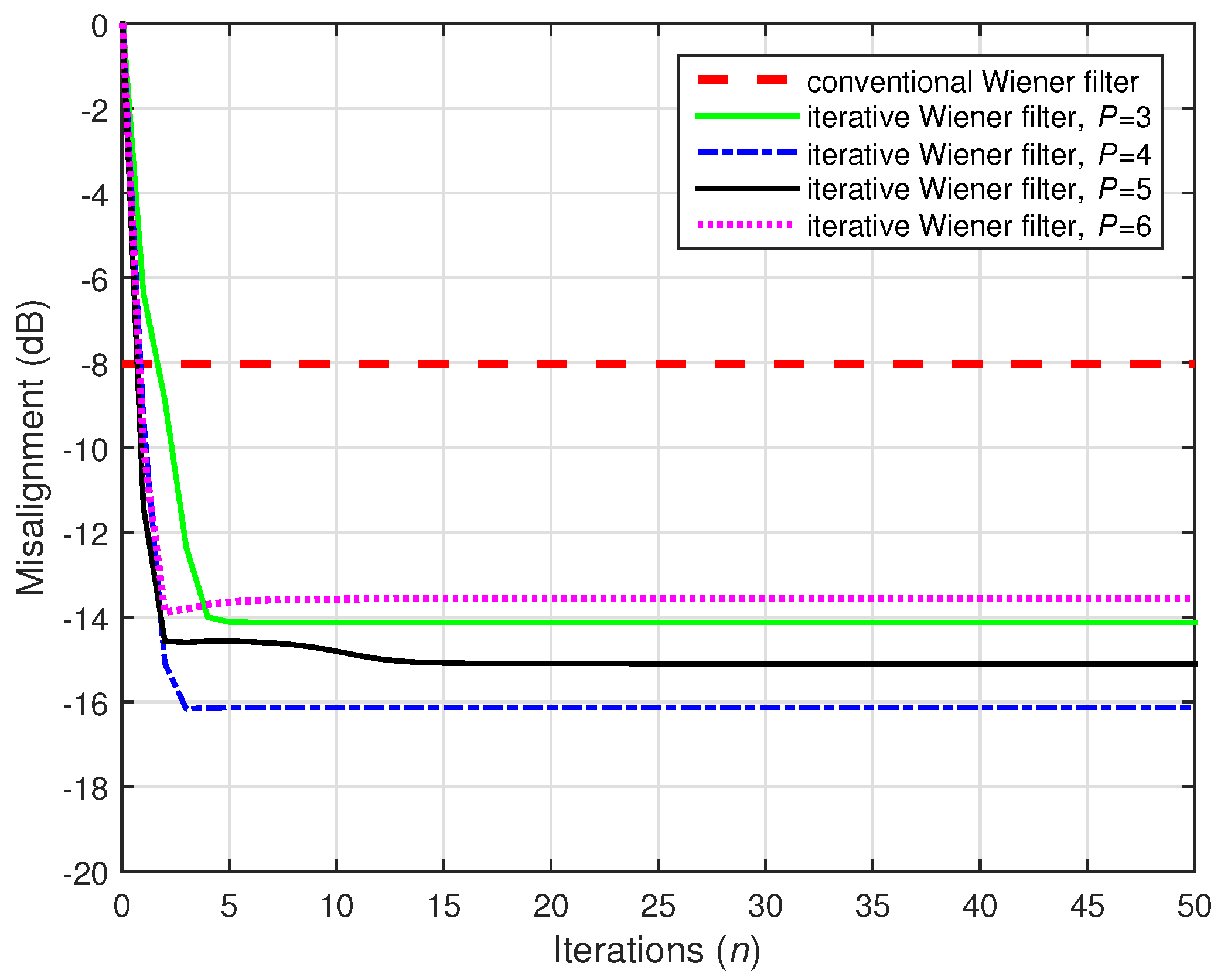
The SNR is also a critical factor in system identification problems. As shown in Figure 7, the performance of the conventional Wiener filter is highly influenced by the SNR level. In the following simulations from this first set of experiments, we considered a more challenging environment, by setting $\mathrm{SNR}=10$ dB. In this case, even for a large amount of data (i.e., $N=$ 10,000), the conventional Wiener filter was outperformed by the iterative version, as supported in Figure 12.

The gain becomes more apparent when fewer data are available to estimate the statistics. Such a case is considered in Figure 13, where $\mathrm{SNR}=10$ dB and $N=2500$. As we can see, the conventional Wiener filter could not provide an accurate solution (as also indicated in Figure 7), whereas its iterative counterpart still attenuated the misalignment to an acceptable degree.

As previously explained (related to Figure 10 and Figure 11), using $N\le ML$ represents a critical scenario for the conventional Wiener filter. In this context, a lower SNR level made the situation even more challenging. Nevertheless, the iterative Wiener filter is reasonably robust even in these adverse conditions. This behavior is supported in Figure 14 and Figure 15, where $N=2000$ and 1500, respectively. The same noisy conditions were considered, with $\mathrm{SNR}=10$ dB. As we can see in these figures, the best behavior was obtained for $P=3$, which is significantly lower than $L_2=20$.

Finally, the last simulation of the first set of experiments was performed in "extreme" SNR conditions, using $\mathrm{SNR}=0$ dB. As we already know from Figure 7, the conventional Wiener filter cannot provide an accurate solution in this case, despite the value of N. In Figure 16, $N=$ 10,000, and $\mathrm{SNR}=0$ dB. As expected, the conventional Wiener filter failed to provide an accurate estimate. On the other hand, the iterative Wiener filter was able to reach a much lower misalignment level, using $P\ll L_2$. Therefore, it is much more robust in noisy conditions, which are frequent in practice.

The second set of experiments was performed in a more challenging situation that appeared in the context of stereophonic acoustic echo cancellation (SAEC) [65,66,67,68]. There were two acoustic echo paths to identify (for each microphone); i.e., $M=2$. Consequently, the reference (or microphone) signal resulted in

$$\begin{array}{cc}\hfill d\left(k\right)& ={\mathbf{h}}_{\mathrm{R}}^T{\mathbf{x}}_{\mathrm{R}}\left(k\right)+{\mathbf{h}}_{\mathrm{L}}^T{\mathbf{x}}_{\mathrm{L}}\left(k\right)+w\left(k\right)\hfill \\ \hfill & =\left[\begin{array}{cc}{\mathbf{h}}_{\mathrm{R}}^T& {\mathbf{h}}_{\mathrm{L}}^T\end{array}\right]\left[\begin{array}{c}{\mathbf{x}}_{\mathrm{R}}\left(t\right)\hfill \\ {\mathbf{x}}_{\mathrm{L}}\left(k\right)\hfill \end{array}\right]+w\left(k\right),\hfill \end{array}$$

(83)

where ${\mathbf{h}}_{\mathrm{R}}$ and ${\mathbf{h}}_{\mathrm{L}}$ correspond to the loudspeaker-to-microphone acoustic impulse responses (right and left, respectively), and ${\mathbf{x}}_{\mathrm{R}}\left(k\right)$ and ${\mathbf{x}}_{\mathrm{L}}\left(k\right)$ comprise the loudspeaker signal samples (right and left, respectively).

At first glance, from a system identification perspective, we need to identify the global impulse response ${\left[\begin{array}{cc}{\mathbf{h}}_{\mathrm{R}}^T& {\mathbf{h}}_{\mathrm{L}}^T\end{array}\right]}^T$. Nevertheless, in an SAEC scenario, the difficulty is many-fold. One of the main challenges is the so-called nonuniqueness problem [66,67], which comes from the fact that the loudspeaker (input) signals are linearly related. This issue can be addressed by manipulating the signals transmitted to the receiving room, e.g., using a preprocessor on the loudspeaker signals to make them less coherent, without affecting the stereo perception and the signal quality much. A simple but efficient nonlinear method uses positive and negative half-wave rectifiers on each channel, respectively [67]. In this case, the nonlinearly transformed signals become

$$\begin{array}{cc}\hfill {\mathbf{x}}_{\mathrm{L}}^{\prime }\left(k\right)& ={\mathbf{x}}_{\mathrm{L}}\left(k\right)+\alpha \frac{{\mathbf{x}}_{\mathrm{L}}\left(k\right)+\left|{\mathbf{x}}_{\mathrm{L}}\left(k\right)\right|}{2},\hfill \end{array}$$

(84)

$$\begin{array}{cc}\hfill {\mathbf{x}}_{\mathrm{R}}^{\prime }\left(k\right)& ={\mathbf{x}}_{\mathrm{R}}\left(k\right)+\alpha \frac{{\mathbf{x}}_{\mathrm{R}}\left(k\right)-\left|{\mathbf{x}}_{\mathrm{R}}\left(k\right)\right|}{2},\hfill \end{array}$$

(85)

where $\alpha$ is a parameter used to control the amount of nonlinearity; the recommended interval for this parameter is $0<\alpha \le 0.5$ [67]. The distortion parameter $\alpha$ (which controls the amount of nonlinearity) is provided a priori. Clearly, this distortion must be performed in such a way that the quality of the signals and the stereo effect are not degraded. Experiments reported in [67] (and also in many subsequent works) show that stereo perception is not affected even with an $\alpha$ as large as 0.5. Additionally, the audible distortion is small because of the psychoacoustic masking effects [69].

However, we should note that other methods can be used to address the nonuniqueness problem; e.g., see [70,71] and the references therein. An analysis of their influences on the overall performance of the decomposition-based approach is beyond the scope of this paper.

In our simulations, the source signal (in the transmission room) was white Gaussian noise. The acoustic impulse responses in the transmission room had 2048 coefficients. The acoustic impulse responses in the receiving room had $L=1024$ coefficients, as depicted in Figure 4. The background noise $w\left(k\right)$ (in the receiving room) was white and Gaussian, with $\mathrm{SNR}=30$ dB.

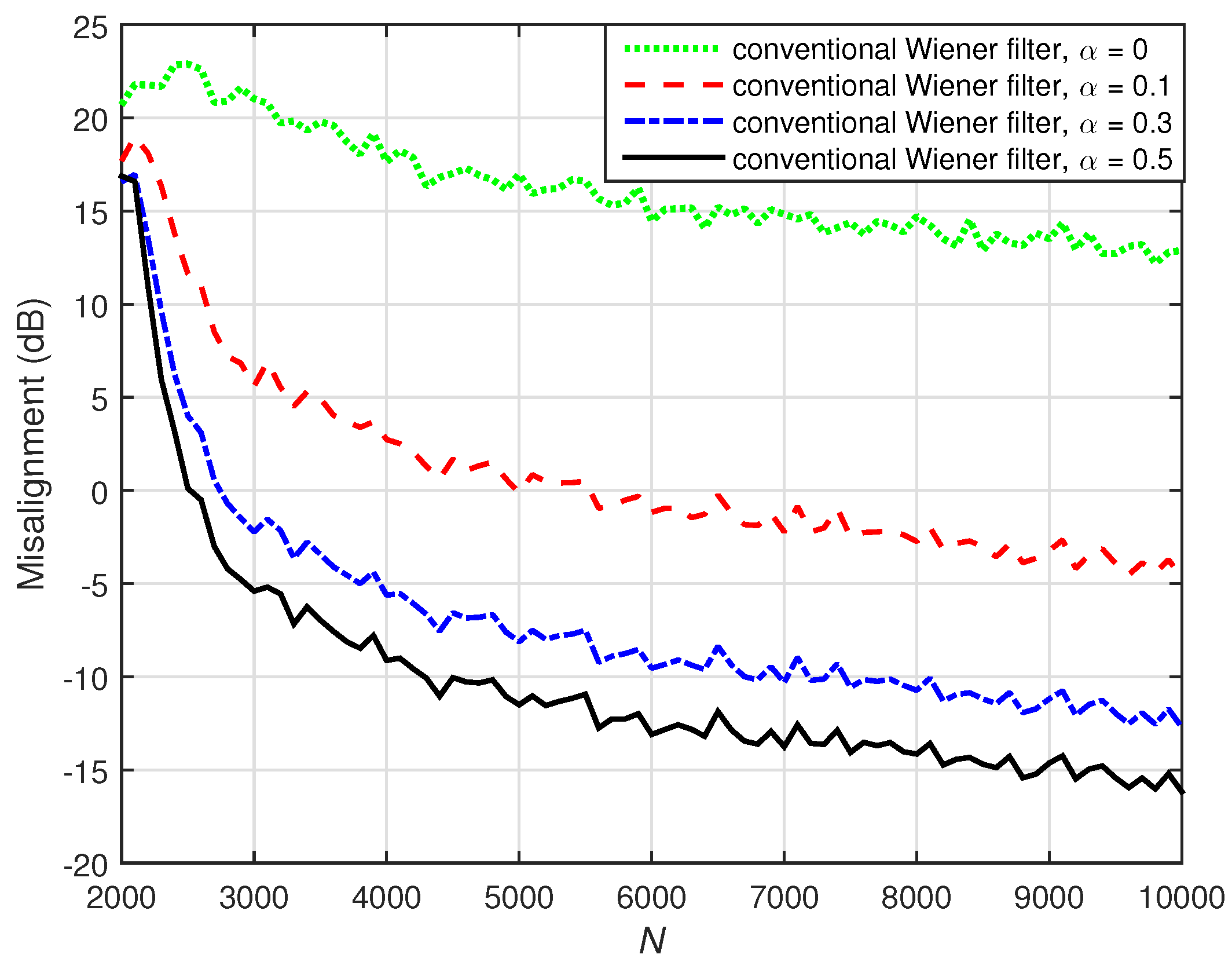
The influence of the preprocessing technique from (84) and (85) on the loudspeaker signals can be seen in Figure 17, where the performance of the conventional Wiener filter is evaluated for different values of N (i.e., the available amount of data used to estimate the statistics) and using different values of $\alpha$, which acted as a distortion parameter. First, we can notice that the performance was clearly improved when preprocessing the input signals using positive and negative half-wave rectifiers with larger values of $\alpha$. Additionally, even with preprocessing, a large amount of data (i.e., $N\gg ML$) is required for the conventional Wiener filter, in order to obtain reasonable misalignment attenuation.

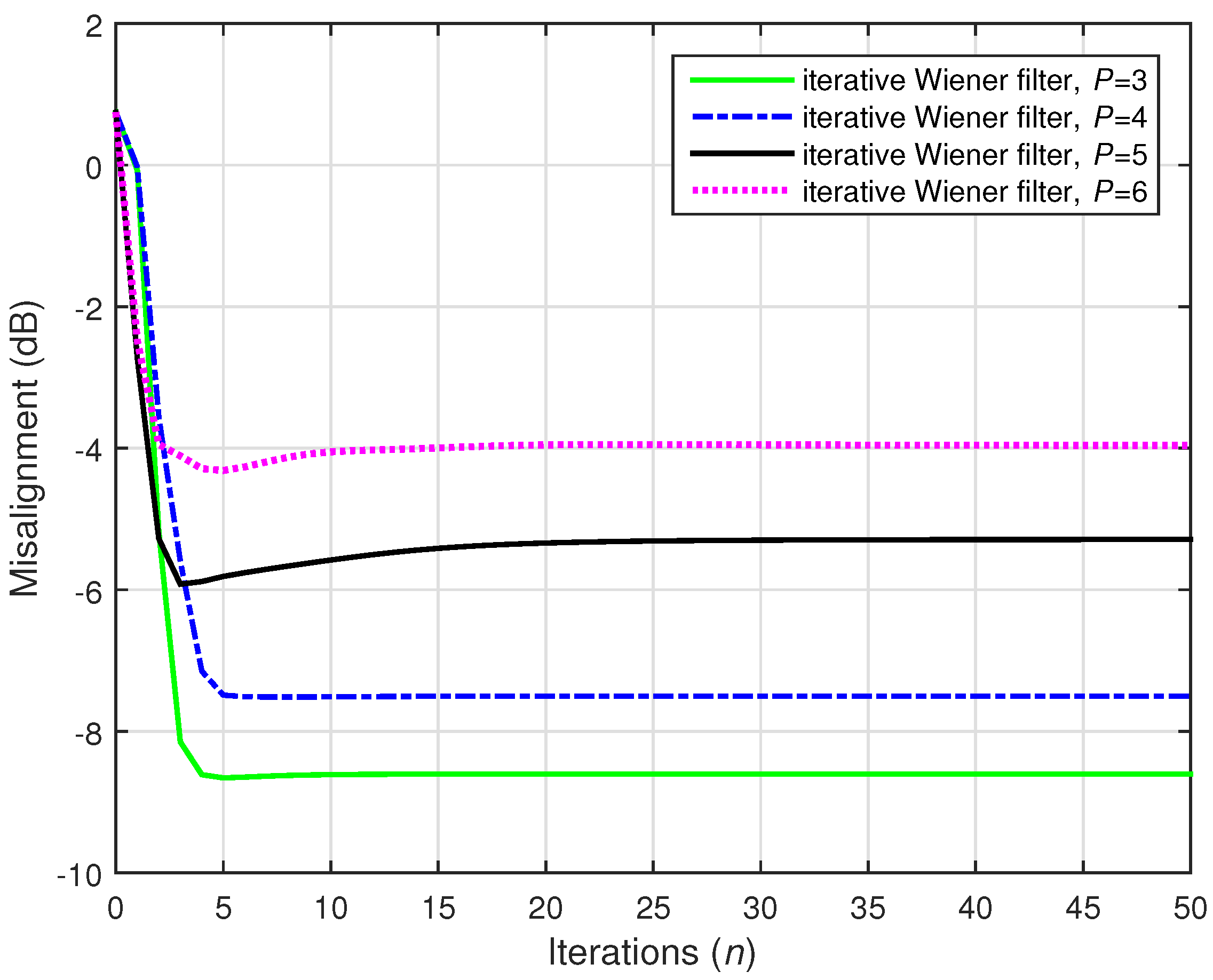
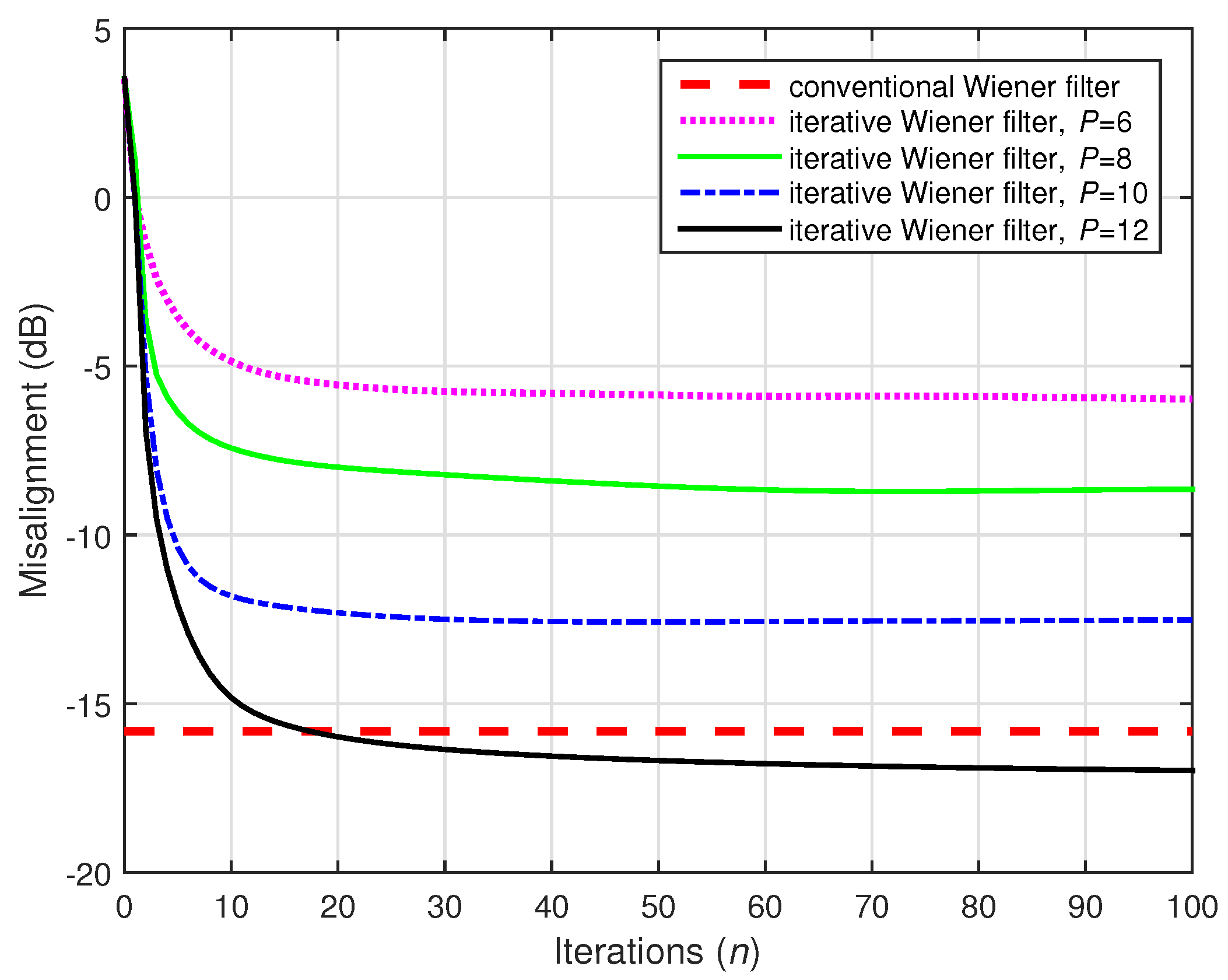
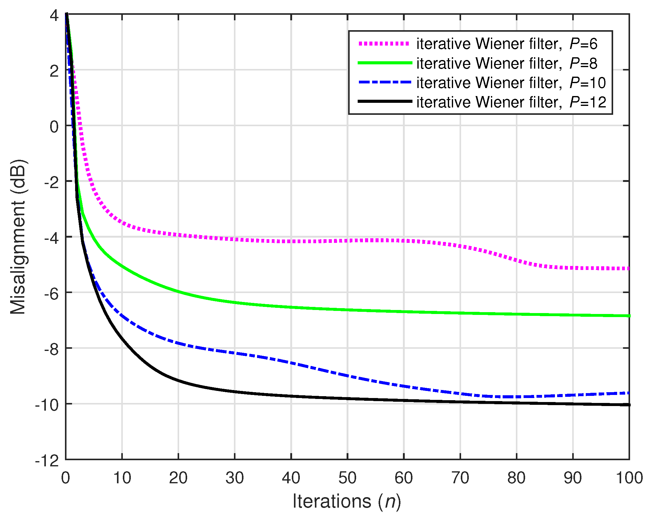
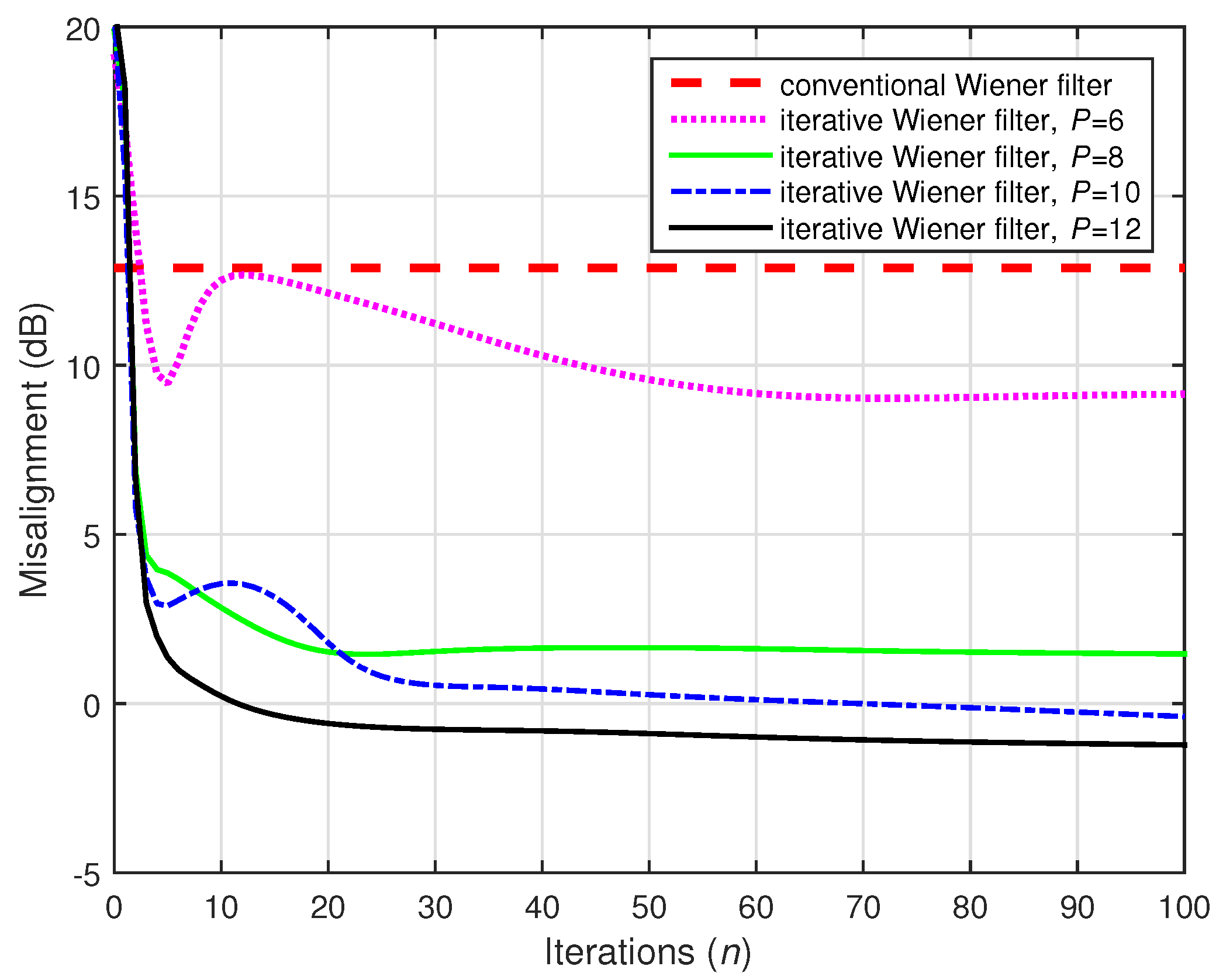
In the following simulations, the identification problem was addressed using the conventional and iterative Wiener filters. The length of the global impulse response was $L=L_1{L}_2=1024$, so that we set $L_1=L_2=32$. Due to the nature of acoustic impulse responses, the matrix $\mathbf{H}$ (or ${\mathbf{H}}_{\mathrm{st}}$) was closer to full rank, so a higher value of P was required. In this context, the iterative Wiener filter involved in the experiments used $P=6,8,10$, and 12. Nevertheless, these values are lower than $L_2=32$.

For the results shown in Figure 18, $N=$ 10,000 data samples were used to estimate the statistics, and the input signals were preprocessed using positive and negative half-wave rectifiers, with $\alpha =0.5$. These represent favorable conditions for the identification, so the conventional Wiener filter had good accuracy (as also indicated in Figure 17). The performance of the iterative Wiener filter was improved for a larger value of P and even outperformed the conventional filter in the case of $P=12$.

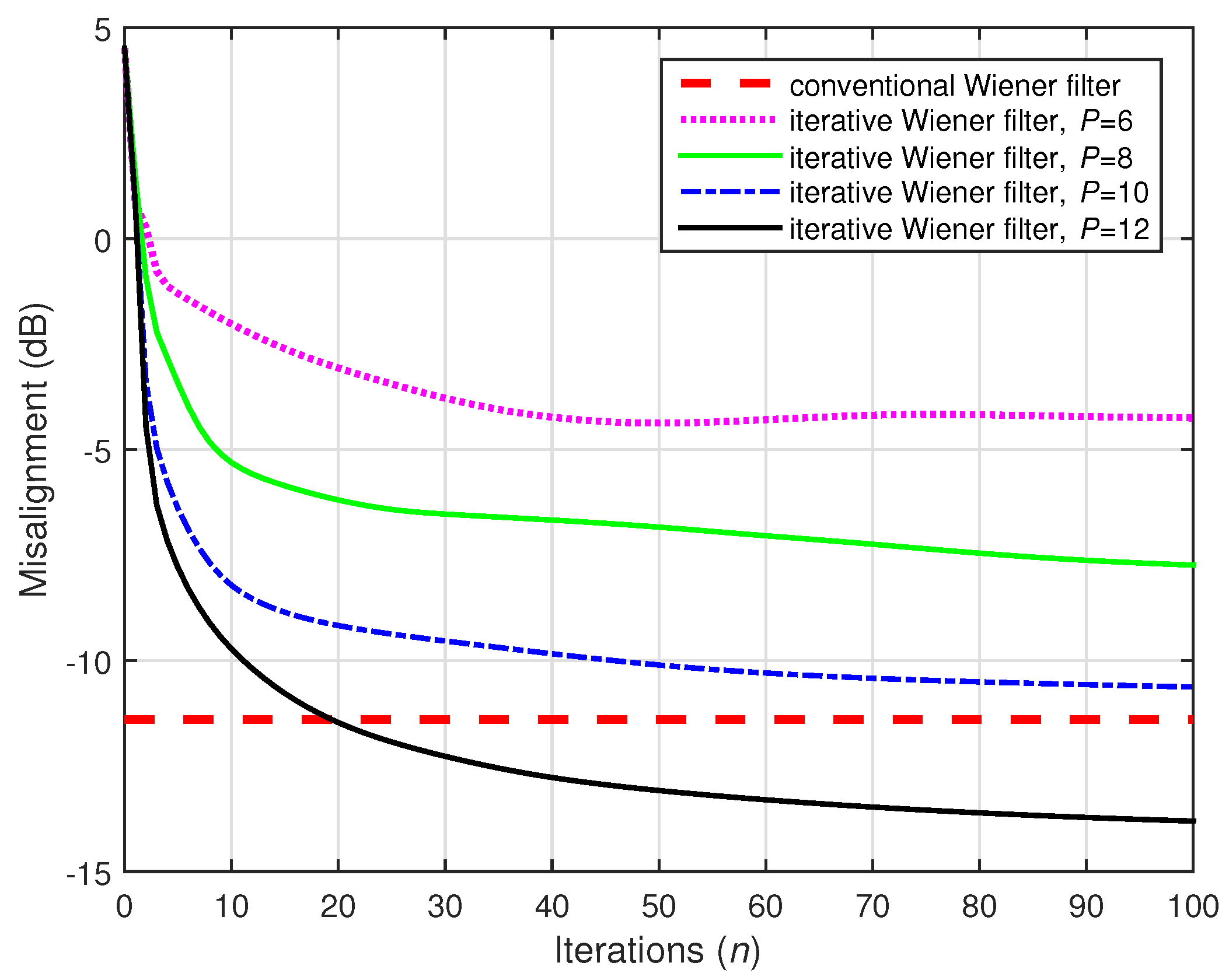
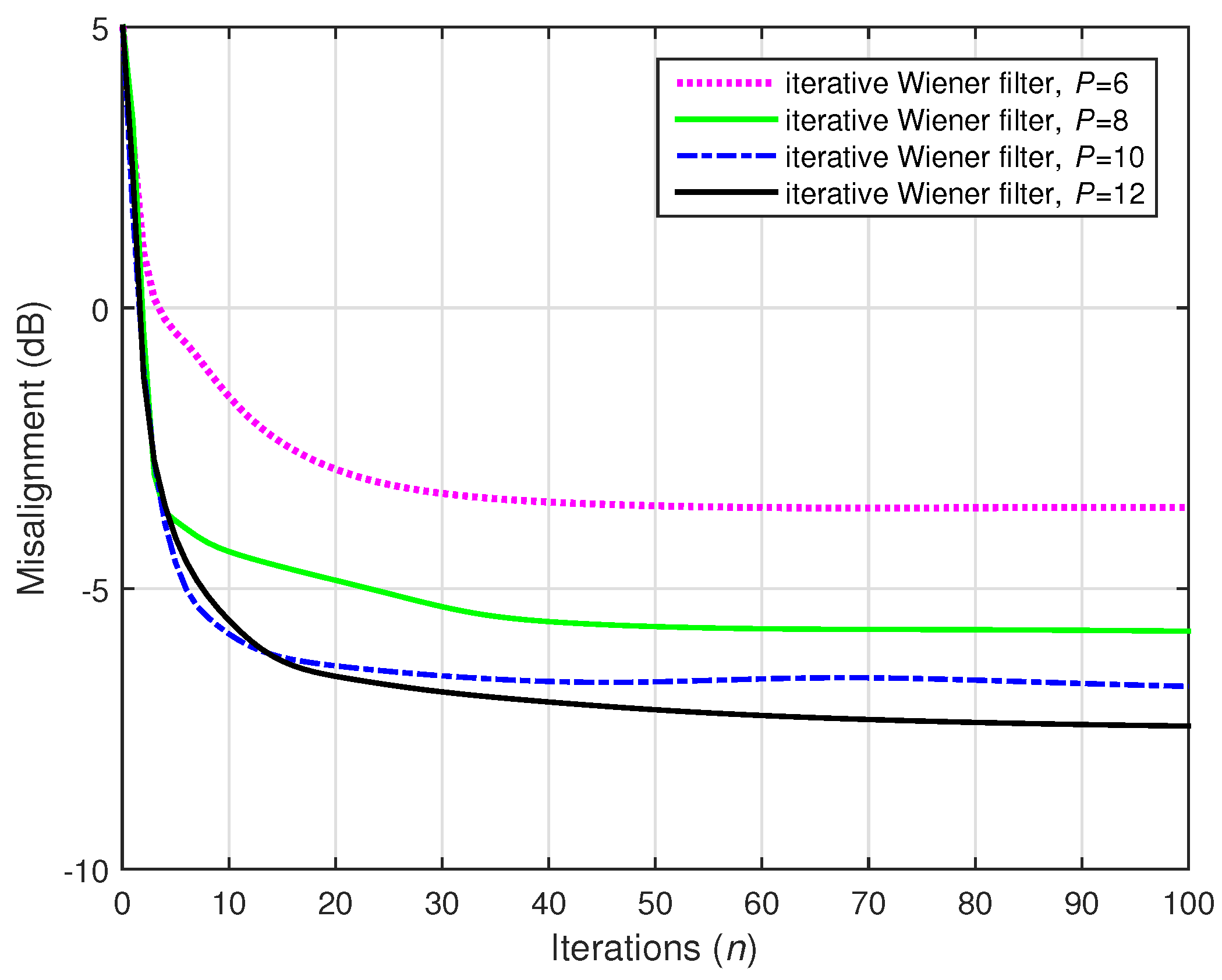
Reducing the value of the distortion parameter influenced the performance for the conventional and the iterative Wiener filters, as shown in Figure 19, where $N=$ 10,000 and $\alpha =0.3$. However, the iterative Wiener filter is more robust to this modification, since for $P=12$ it outperformed the conventional benchmark, and for $P=8$ it reached a misalignment level close to the conventional Wiener solution.

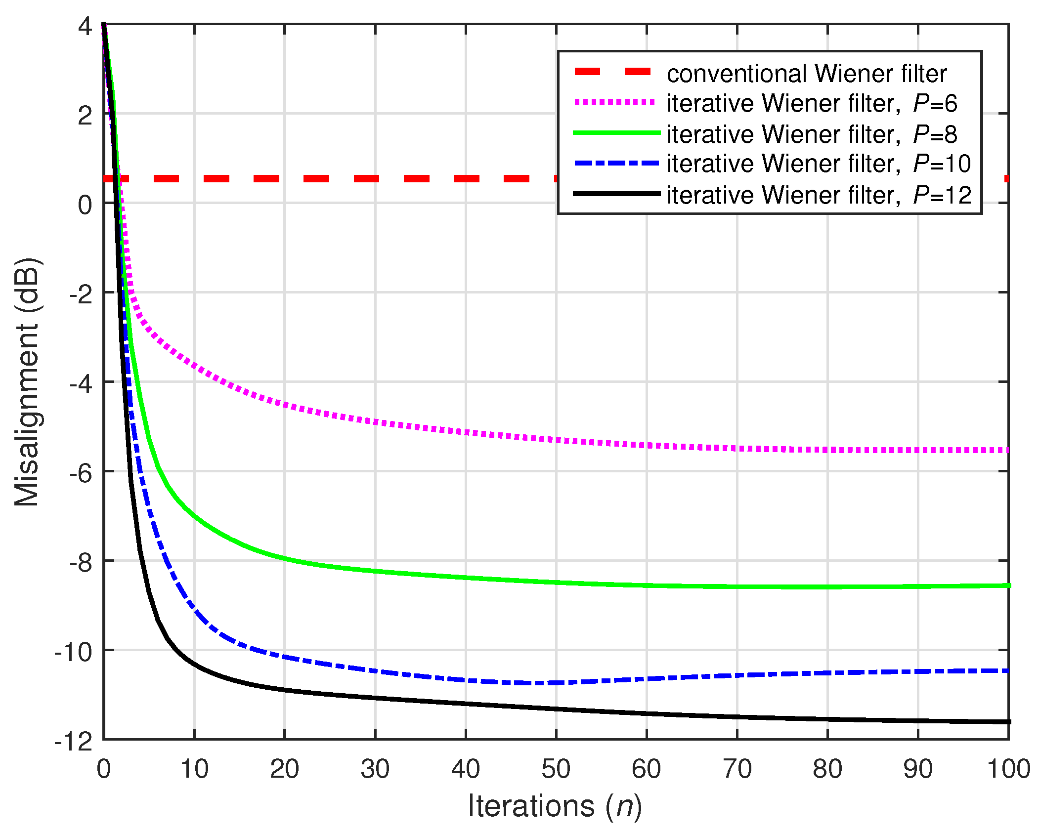
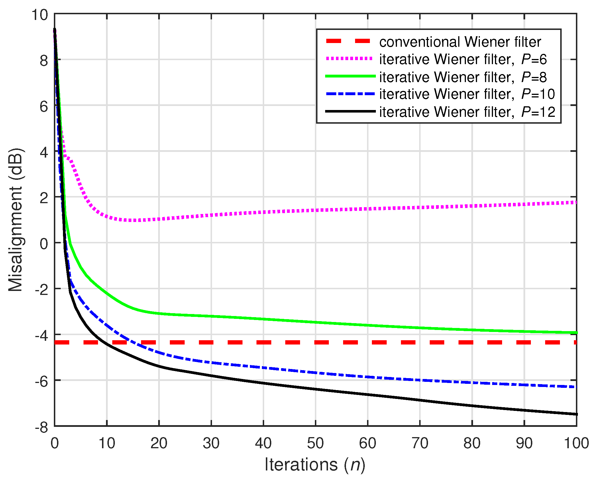
Next, for the simulations shown in Figure 20 and Figure 21, less data were used to estimate the statistics—i.e., $N=2500$. The other conditions were the same as in Figure 18 and Figure 19, respectively. As we can notice, the conventional Wiener filter could not obtain an accurate solution in these cases, despite the value of the distortion parameter. On the other hand, the iterative Wiener filter was still able to achieve reasonable results (for $P<L_2$), thereby far outperforming the conventional solution. The difference was even more apparent for a lower value of $\alpha$, as supported in Figure 21.

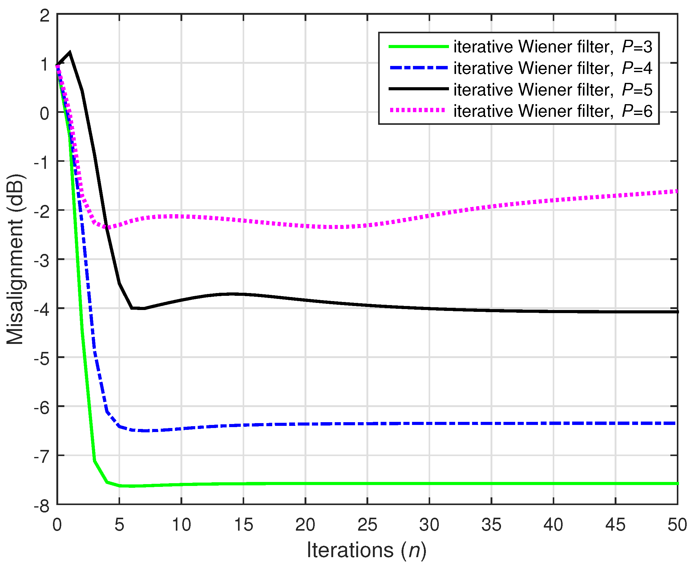
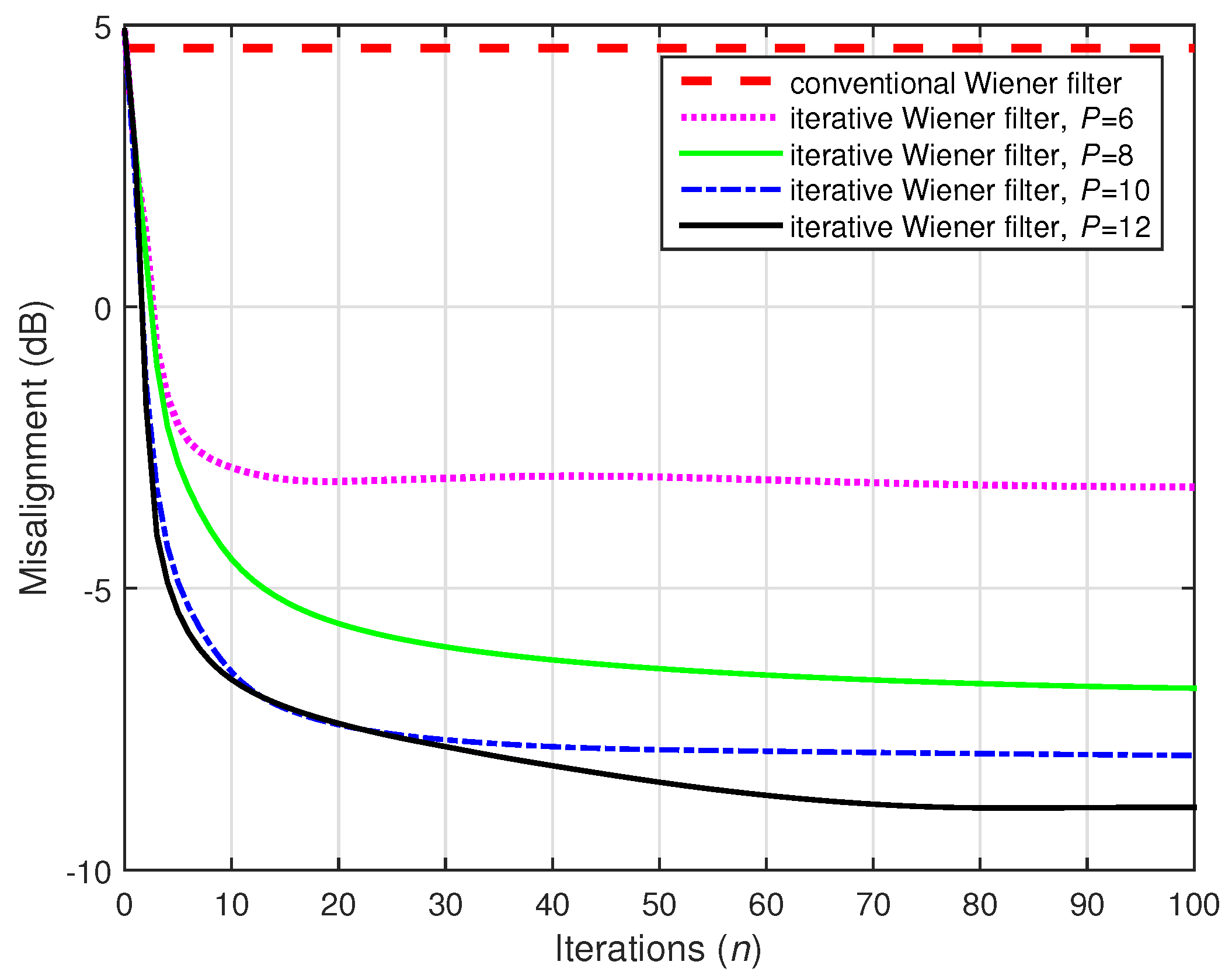
A challenging case $N<ML$ was considered in the following two simulations, where we set $N=2000$ (while $ML=2048$). Two values of the distortion parameter were considered, i.e., $\alpha =0.5$ and $0.3$, and the results are depicted in Figure 22 and Figure 23, respectively. The conventional Wiener filter was not included in these experiments, since it could not provide an accurate solution (as indicated in Figure 17). As we can notice in both cases, despite the adverse conditions, the iterative Wiener filter was still able to attenuate the misalignment to a reasonable extent and provide a robust solution, for a value of P smaller than $L_2$.

As shown in Figure 17, the conventional Wiener filter could not obtain an accurate solution for small values of the distortion parameter $\alpha$ (i.e., closer to 0). For example, when using $\alpha =0.1$, its misalignment could not reach $-5$ dB even with a large amount of data (i.e., $N=$ 10,000); and for less data (e.g., $N=2500$), it provided a far from accurate solution. These cases are considered in Figure 24 and Figure 25, using $\alpha =0.1$; $N=$ 10,000 and 2500, respectively. For N = 10,000 (Figure 24), the iterative Wiener filter outperformed the conventional solution for $P=10$ and 12. The decomposition using $P=8\ll L_2$ reached the misalignment level provided by the conventional Wiener filter. However, the differences (in favor of the iterative version, for all the values of P) were significant when $N=2500$, as supported in Figure 25.

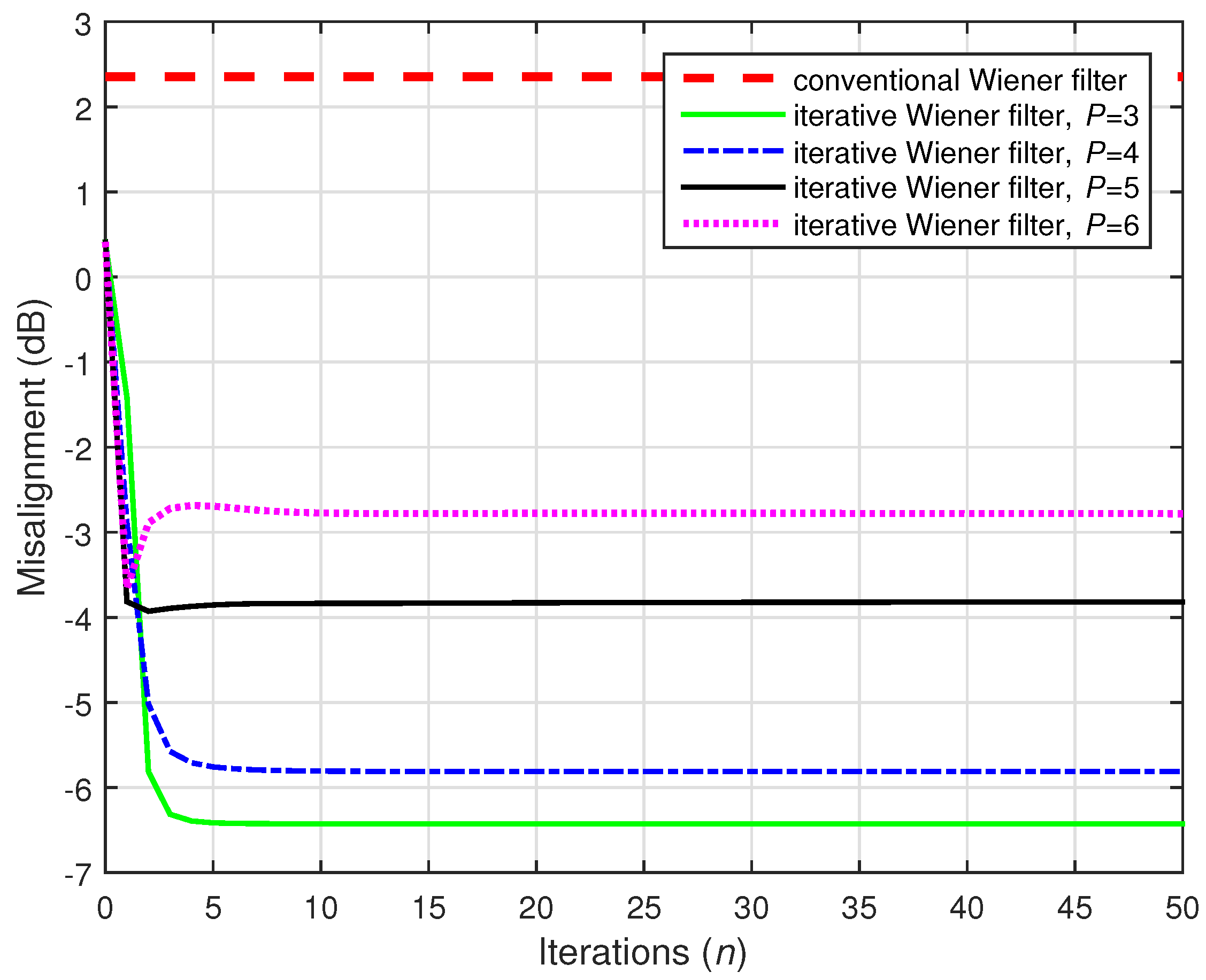
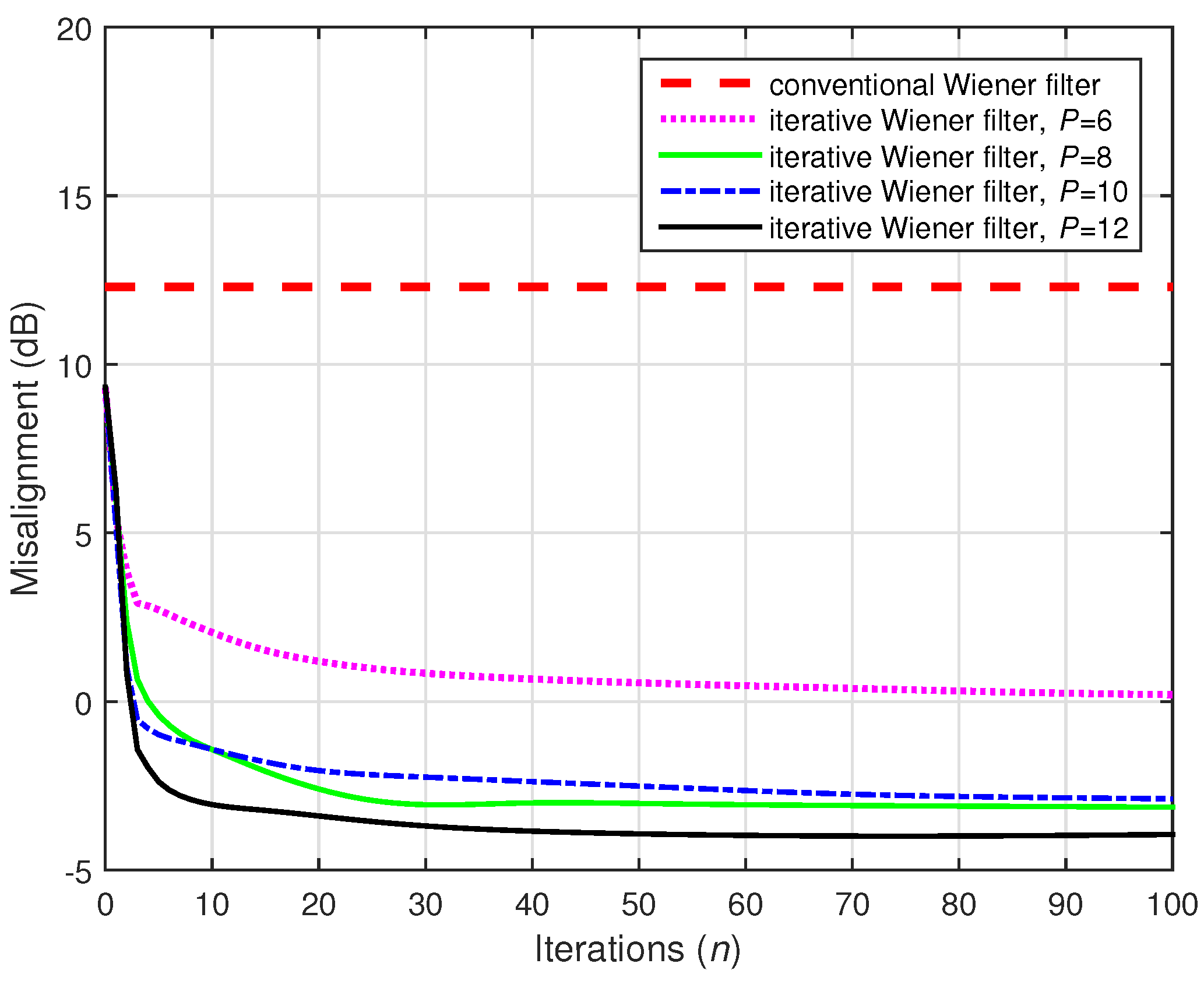
Finally, as shown in Figure 26, $N=$ 10,000 data samples are used to estimate the statistics, but the input signals were not preprocessed (i.e., $\alpha =0$). Even if $N\gg ML$, the conventional Wiener filter could not obtain an accurate solution in this case. On the other hand, the iterative Wiener filter with $P\ll L_2$ was able to outperform the conventional Wiener solution, even in this extremely difficult scenario. In other words, the influence of the nonuniqueness problem is less significant for the iterative Wiener filter. This is probably due to the fact that the matrices within the iterative Wiener filter are smaller as compared to the full matrix of size $ML\times ML$ within the conventional Wiener filter.

Summarizing, the main feature of the multichannel iterative Wiener filter is that it operates with smaller data structures, i.e., of size $PM{L}_1$ and $P{L}_2$, with P values far smaller than $L_2$. On the other hand, the conventional Wiener filter addresses a system identification problem of size $L=L_1{L}_2$. In our experiments, we tried to cover a wide range of scenarios, in order to properly assess the performance of the multichannel iterative Wiener filter, as compared to its conventional counterpart. Consequently, we used different values of N (the available data to estimate the statistics), different noise levels (SNR), and different values of the decomposition parameter P. Moreover, in the SAEC scenario, we also used different values of the distortion parameter $\alpha$. As an overall conclusion, the iterative version significantly outperformed the conventional Wiener filter, especially in difficult conditions and environments, e.g., when using small amounts of data or low SNRs. These scenarios are of great importance in practice, as in real-world applications, only small amounts of data may be available (to estimate the statistics) or the filters may need to operate in noisy environments.

7. Conclusions and Perspectives

In this review paper, we have addressed the system identification problem from an efficient decomposition-based perspective. The contributions are threefold. First, we have shown how the main categories of linear SISO and MISO systems can be interpreted and related in a unified framework, taking advantage of the bilinear form representation. Second, we have demonstrated that the resulting spatiotemporal impulse response of the MISO system can be efficiently identified using the nearest Kronecker product decomposition, followed by low-rank approximations. Third, we have developed an iterative Wiener filter based on these techniques which outperforms the conventional Wiener filter in terms of accuracy and robustness of the solution. The main feature of the overall approach consists of an efficient (re)formulation of a high-dimension system identification problem (e.g., identification of a long spatiotemporal impulse response) as a combination of low-dimension solutions, which result from the optimization of shorter component filters.

In this study, we have illustrated the performance of the decomposition-based approach only in terms of the Wiener filter, which represents a benchmark tool for system identification problems. Simulation results have indicated that the iterative version is able to outperform the conventional Wiener filter, especially when a small amount of data is available for the estimation of the statistics. This represents an important performance feature, taking into account that in many real-world applications we deal with incomplete information related to the inputs/outputs of the system.

In perspective, improved solutions based on adaptive filtering should also be developed, which could further extend the applicability of the decomposition-based approach. For example, several preliminaries toward this goal can be found in [44,45]. Furthermore, a rigorous convergence analysis of these algorithms could reveal the influence of the decomposition parameters, which could be further exploited in order to improve the overall behavior. In addition, finding a practical method to determine the optimal value of the decomposition parameter P represents one of our main tasks for future works. Nevertheless, this is not a straightforward task, since the decomposition parameter depends on the nature of the system to be identified (which is unknown in practice). However, we can take advantage on some a priori knowledge of the system. For example, in the case of network echo paths (which are usually very sparse), the value of P is much smaller than $L_2$. For acoustic impulse responses, the value of P should be increased, but it must still be considerably lower than $L_2$. A preliminary study on the influence of the decomposition parameter can be found in [43].