Article

Sequence to Point Learning Based on an Attention Neural Network for Nonintrusive Load Decomposition

School of Economics and Management, China University of Mining and Technology, Xuzhou 221116, China
*
Author to whom correspondence should be addressed.
Electronics 2021, 10(14), 1657; https://doi.org/10.3390/electronics10141657
Submission received: 18 May 2021 / Revised: 7 July 2021 / Accepted: 8 July 2021 / Published: 12 July 2021
(This article belongs to the Special Issue Smart Processing for Systems under Uncertainty or Perturbation)

Abstract

:
Nonintrusive load monitoring (NILM) analyzes only the main circuit load information with an algorithm to decompose the load, which is an important way to help reduce energy usage. Recent research shows that deep learning has become popular for this problem. However, the ability of a neural network to extract load features depends on its structure. Therefore, more research is required to determine the best network architecture. This study proposed two deep neural networks based on the attention mechanism to improve the current sequence to point (s2p) learning model. The first model employs Bahdanau style attention and RNN layers, and the second model replaces the RNN layer with a self-attention layer. The two models are both based on a time embedding layer. Therefore, they can be better applied in NILM. To verify the effectiveness of the algorithms, we selected two open datasets and compared them with the original s2p model. The results show that attention mechanisms can effectively improve the model’s performance.

1. Introduction

Nonintrusive load monitoring (NILM) is the decomposition of the status and power consumption of individual appliances according to the overall load information at the user’s power supply entrance. The concept was first proposed by G. W. Hart in the 1980s [1]. NILM is of great value to power suppliers, intermediaries, and end users. With the rapid development of smart grids and smart homes, many new opportunities have arisen for achieving efficient energy utilization through big data and two-way controllable appliances. In traditional load decomposition methods, appliances are identified by analyzing the signal characteristics of the voltage and current, which are also referred to as the load signatures. Based on the load signatures of the appliances, load decomposition can be realized through load identification algorithms [2,3,4,5]. According to the working conditions of appliances, load signatures can be divided into three types: steady-state, transient state, and operating state. The various characteristics of load signatures repeatedly appear over time. The periodic pattern is used to identify the load type [6]. A typical load decomposition process includes five steps: data measurement, data processing, event detection, feature extraction, and load identification [7]. By comparing the load features of an event with data from the appliance load characteristics database, the appliances can be identified. Currently, there are two main methods for the construction of a load characteristics database [8]. The first is to record the load characteristics of each appliance manually, and the other is completed via an automatic classification algorithm. The remarkable achievements of deep learning technology in image recognition and speech recognition have inspired researchers to apply this approach to load decomposition [9,10].
According to the acquisition frequency, data in NILM studies can be divided into high-frequency (less than 1 s) and low-frequency (a few seconds to a few hours) data. The sampling period of 1 s can be used as the threshold to distinguished the macroscopic and microscopic characteristics [10]. High-frequency data preserve the entire signals and therefore allow us to extract the maximum information content. Nevertheless, the cost of gathering high frequency data constitutes a major obstacle. On the other hand, the loss in information intrinsic in low frequency features is offset by the tremendous ease with which those data can be collected [11]. Roll-out smart meters [12] can export low frequency data to the outside, which can be tackled using low frequency approaches. Therefore, low frequency data will most likely be the only one available at scale in the near future [11]. According to Pereira et al. [13], NILM can be divided into two categories based on different task purposes: event detection (ED) and energy estimation (EE). ED mainly predicts the switch state of appliances, and EE mainly predicts the power consumption. NILM methods based on ED are referred to as event-based solutions [9], which detect the turning-on of a target appliance by processing the measured active power transient response and can estimate its consumption in real-time [14]. In contrast, the methods directly perform energy decomposition without ED are thus referred to as event-free. The event-based methods depend on precise event characteristics; therefore, these methods are appropriate for high-frequency data. In addition, the event-free methods without identifying the state of appliances are more suitable for low-frequency data.
Kelly et al. [15], proposed three deep neural network architectures for NILM: long short-term memory (LSTM), denoising autoencoders (DA), and rectangles, which were verified using the open dataset UK-DALE [16]. Recent studies have proved that Convolutional Neural Network (CNN) can also accomplish the NILM task [17], and it can be used together with the LSTM network [18]. The results showed that the deep neural network model was superior to the traditional combinatorial optimization (CO) and factorial hidden Markov model (FHMM) model. However, LSTM cannot learn from equipment with long power changing intervals, leading to a vanishing gradient [19,20]. Sequence-to-sequence (s2s) is a general end-to-end training method that can map sequences to sequences, first proposed to tackle text translation problems [21]. This model used the LSTM network as an encoder to compress the input sentence into a fixed-length context vector. The context vector information was then decoded with the encoder to generate the output sentence. This model significantly improved translation accuracy. Kelly et al. [15] showed that the s2s model could effectively identify the target appliances from the overall load power signal. Xia [22] proposed an improved s2s model that reduced the difficulty of learning long time-series data by increasing the receptive field and capturing more data through a dilated convolution network.
The sliding window method is usually applied to the s2s model to produce the input and output sequences. Sequence to point (s2p) different from the s2s means the network map from an input sequence to a single output value. It is only used if the output of the network is active power or the on/off state of an appliance [11]. Zhang et al. [23] proposed an s2p model, in which the input is the window of the main power signal and the output is a single point of the target appliance. If [ X ( t ) ~ X ( t + w 1 ) ]   represents the input window sequence of the model at time t, then the s2p model can only predict the output at time t + (w/2), which allows the neural network to focus on the midpoint of the window while fully utilizing the information of the front and rear adjacent areas, thereby improving the prediction accuracy. Jia [24] proposes an s2p learning framework based on bidirectional (non-casual) dilated convolution for NILM. Sudoso [25] proposes a deep neural network that combines a regression subnetwork with a classification subnetwork to solve the NILM problem. The proposed model employs s2s with a tailored attention mechanism in the regression subnetwork to detect and assign more importance to the turning on-off events, whereas the classification subnetwork helps the disaggregation process by enforcing explicitly the on/off states. It is essentially an ED solution for NILM. Both experiment results show outperforms s2p (Zhang), but they do not publish their codes. In this study, we propose two s2p models based on the attention mechanism for EE. The one employs the Bahdanau style attention mechanism to improve a conventional s2p model, including two recurrent neural network (RNN) units as encoder and decoder. The other replaces the RNN layer with the self-attention layer to shorten training time and improve prediction accuracy. Experiments on the public datasets show that the proposed model performs better at NILM than existing s2p models. In addition, we also compared the s2s and s2p learning methods based on the model structure proposed in this paper. The results show that s2p is more suitable for solving the NILM problem.

2. Deep Neural Network Based on the Attention Mechanism

2.1. Attention Mechanism

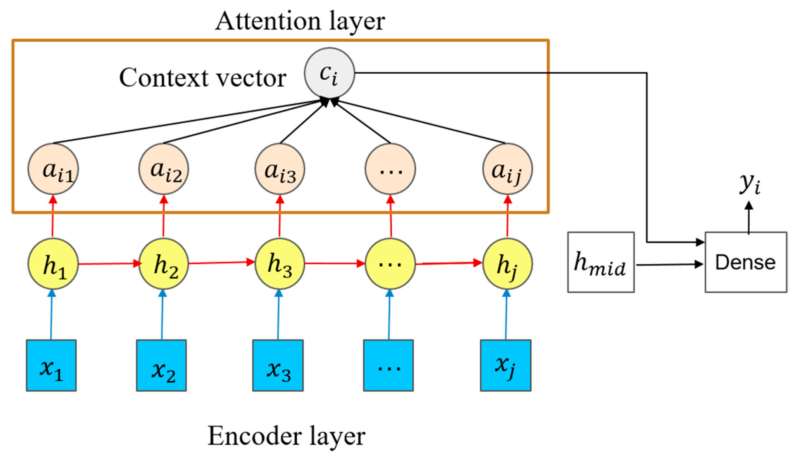
The attention mechanism is also referred to as the attention model and is similar to the way the human brain automatically ignores unimportant information, focusing on important information. The core idea is to calculate and distribute the attention weight, and the focus is placed on important content by increasing its weight. This addresses the problem of the s2s model losing information when the input sequence is too long. Taking a typical machine translation scenario as an example, the s2s model only uses the final hidden state of the input sentence to calculate the context vector, while the attention model calculates the individual context vector for each word of the input sentence, and therefore, more information is retained for the decoder. Bahdanau et al. [26] solved the problem of the input sentence being compressed into a fixed context vector in the s2s model by allowing the model to automatically (soft) search for the part of the original sentence related to the predicted target word to translate (prediction), implementing a variable context vector, and proposing the first attention mechanism. The encoder of the new architecture calculated the context vector relative to each word, while the attention layer converted the context vector into weights and performed pointwise multiplication to obtain a new context vector to send to the decoder. The input of the decoder consisted of two parts: the hidden state of the previous moment and the context vector of the dynamic calculation. Moreover, a bidirectional RNN was used as the encoder of the s2s model, which exhibited relatively good performance in extracting contextual information. Figure 1 describes the working principle of the Bahdanau attention mechanism.
The output at time i is presented by y i = g ( y i 1 , s i , c i ) , where s i is the hidden state of decoder, computed by s i = f ( s i 1 ,   y i 1 ,   c i ) . The context vector c i which is the weighted summation of the attention weight a i j and the hidden state h j of the encoder, as shown in Formula (1). The attention weight a i j is calculated as shown in Formula (2) and represents the correlation between the j-th position of the input sequence and the i-th position of the output sequence. e i j is referred to as the attention score, which is based on the hidden state s i 1 of the decoder and the j-th annotation h j of the input sequence as shown in Formula (3), where v , W 1 and W 2 are the parameter matrices, which are determined via model training.The method using the previous hidden state of the decoder to compute attention score is called Bahdanau style. In this study, we employ the Bahdanau attention mechanism to improve the s2p learning model.
c i = j = 1 T x a i j h j
α i j = e x p ( e i j ) k = 1 T x e x p ( e i k )
e i j = v t a n h ( W 1 s i 1 + W 2 h j )
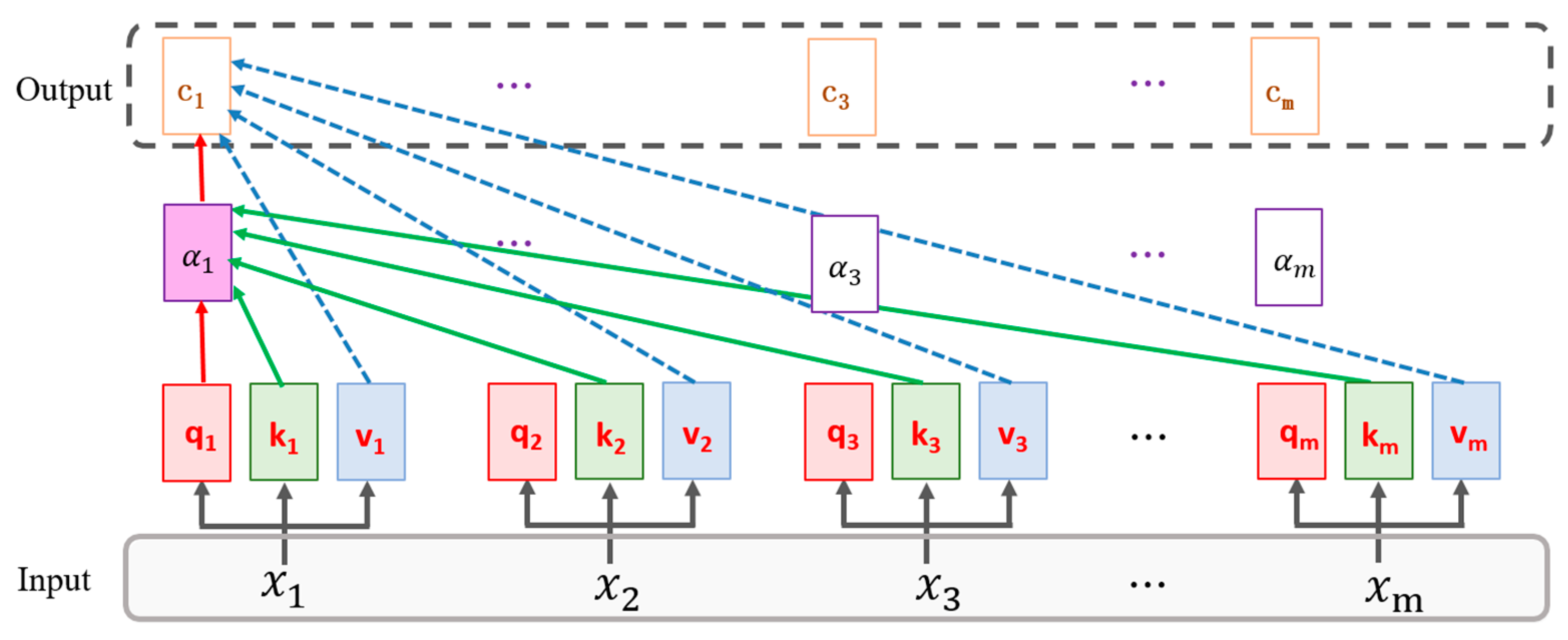
The output from the attention layer contains the information required at the source when forecasting the output. By contrast, self-attention proposed by [27], captures the internal dependency relationship between the sequence elements at the source and the internal dependency relationship between sequence elements at the target separately. Therefore, self-attention is more effective than conventional attention, which neglects the dependency relationship between the source or target elements. The working principle of self-attention is shown in Figure 2. First, q , k , and v are obtained by linearly transforming the input sequence x , and the attention score of x is obtained as the dot product of q and K T . In particular, K denotes a matrix composed of k 1 to k m , as shown by the green solid line. The attention weight α obtained by the softmax operation of attention score shows the internal dependency relationship of the input sequence. The matrix c obtained from the dot product of α and V is the context vector, whereas V denotes a matrix composed of v 1 to v m , as shown by the blue dot line. The details of computation are provided in Formula (4). Moreover, as can be seen from Figure 2, the self-attention layer has the same input and output as an RNN layer and can therefore replace the RNN layer.
{ q = W Q x ; k = W k x ; v = W v x α = s o f t m a x ( K T q ) c = V α

2.2. s2p Model Based on the Attention Mechanism

Depending on the length of the input and output sequences, the s2s model has three forms: many-to-many, many-to-one and one-to-many [21]. But traditional s2s model employs RNN as encoder and decoder, which relies on the output of the last moment for computation. Thus, parallel computing cannot be realized, leading to a very long model training period. The s2p model proposed by Zhang et al. [23] is different from the conventional s2s model because 1D-CNN instead of RNN is employed. Experiments in [23] show that the s2p method achieves the best performance compared with AFHMM (Kolter) [28] and s2s (Kelly) [15]. The s2p (Zhang) model is composed of five 1D-CNN layers and two fully connected layers, as shown in Figure 3. In the present study, we propose two attention models for s2p learning: the s2p+bahdanau attention model and the s2p+bahdanau attention+self-attention model. The former is composed of an embedding layer, a bi-directional GRU encoding layer, an attention layer, a one-way GRU decoding layer, and two fully connected layers. Figure 4 shows the structure of the proposed model. This model employs the bahdanau attention mechanism, but the model’s output is only one point. When training the model, data have to be feed to encoder and decoder, respectively.
The latter uses a self-attention layer to replace the RNN layer. Figure 5 shows the structure of the proposed model. An embedding layer is used to map the input sequence to a higher-dimension space, and the concatenate layer then connects the embedding layer with the original input result and sends the layers to the self-attention layer. The two fully connected layers behind the attention layer replace the decoder for forecasting. Different from the traditional attention model, the s2p+bahdanau attention+self-attention model proposed in this paper removed the RNN layer of decoder, and directly uses dense layer to receive the output of the attention layer. The reason is that the model predicts only one point, so the dense layer will not reduce the prediction accuracy of the model. However, the new network needs to adjust the calculation method of the attention score. As shown in Figure 6, since the decoder hidden state s i 1   no longer exists, we use the hidden state in the middle of the encoder h mid instead. The reason for that is the h mid contains the information for predicting the power of the target appliance at the midpoint of the sequence. The calculation of the context vector is the same as Formulas (1)–(3). In this paper, the effect of the attention model is enhanced by using a time-embedding layer called Time2Vector to process the input sequence [29]. This orthogonal but complementary approach develops a general time vector representation through sine and linear activations. In addition to automatically learning periodic and nonperiodic time features, the Time2Vector can guarantee that these features will not be affected by the time scale. The Time2Vector can be easily embedded in other machine learning models. Experiments on multiple tasks and datasets have demonstrated the efficacy of this method [29].

3. Data and Experiment

3.1. Dataset and NILMTK Toolkit

In this study, two open datasets, REDD and UK-DALE, were used for experiments. The REDD dataset contains six households and 10 to 24 residential appliances in North America [30]. The sampling periods for mains and appliances were 1 s and 3 s, respectively. The UK-DALE dataset consists of over ten types of appliances in five British houses over two years [16]. The mains and appliances were sampled at intervals of 1 s and 6 s, respectively. For comparison, four types of appliances in REDD and five classes in UK-DALE were selected, according to the work of s2p [23]. They are kettle (not available in REDD), microwave, fridge, washing machine and dishwasher. In the experiment, low-frequency active power data was used for decomposition, and the same model network architecture was used for different appliances. In 2014, Kelly [31] developed an open-source toolkit specifically for NILM, which provides a processing interface of mainstream open datasets to simplify NILM data processing tasks. Additionally, the toolkit provides a baseline model and performance metrics, which facilitates the development of state-of-art models [31,32]. The ElecMeter object is the core of the NILM toolkit (NILMTK), encapsulating the method for obtaining power data from the circuit. The mains and submeters at the API interface are called to get the power data of the main electricity meter and its subordinate appliances.
The deep learning model must be trained using data subjected to standard processing to prevent deterioration of the gradient descent efficiency. We obtained the z-score for the experiment by subtracting the mean value from the power of mains or appliances and then divided the result by the standard deviation. The normalizing parameter values according to [23] are shown in Table 1. Due to the different sampling periods of the mains and appliances, we resampled the mains data to mean value according to the appliance’s interval. The data interval was 3 s on REDD and 6 s on UK-DALE, respectively. The sliding window method was applied to obtain the sequence required for model input. Specifically, the time-series data were divided into fixed-length and overlapping windows. One window referred to an input sequence, and the output corresponded to the output power of the appliances to be decomposed at the middle point of the time window. The shape of the input tensor X of the training model was [batch size, window length, 1], and that of the output tensor Y was [batch size, 1]. For the window length and training batch size used in the experiment, see Table 2 below.

3.2. Model Training

In this study, we trained three models for comparison: Model 1 represents the s2p model proposed by Zhang et al. [23]; Model 2 represents the s2p+bahdanau attention model; Model 3 represents the s2p+Bahdanau attention+self-attention model. Figure 3, Figure 4 and Figure 5 show the network structures of the models. The mean squared error (MSE) was used as the loss function in both models, and the Adam algorithm was used to optimize the learning process. The experiment platform was as follows: hardware: Intel Xeon Gold 6230 (base frequency 2.1 GHz), 512 G DDR4 memory, and an NVIDIA Tesla V100 display card (32 GB memory); software: an Ubuntu18.04 64-bit operating system, Python3.7, TensorFlow2.1, cuDNN10.1, and NILMTK0.4.
In REDD, houses 2–5 served as the training set, and house 1 was used as the test set; in UK-DALE, house 1 was the training set, while house 2 was the test set since the data in other houses are small. To deal with the overlong training period, we applied an early-stopping strategy with the specific experimental parameters shown in Table 2. The training time required for five types of appliances varies due to different sample sizes. Because Model 3 proposed herein removed the RNN, it can use graphics processing units (GPUs) for parallel computing, which substantially increases the training speed compared with Model 2. Table 3 shows the comparison of the total parameters and the training time for each model.

3.3. Performance Evaluation

The NILM model can be evaluated in various ways. The mean absolute error (MAE) and F1 score are the most applied performance measures in the case of energy estimation and on/off state classification, respectively [11]. This study chooses MAE and signal aggregate error (SAE) as the metrics, just like [23]. Additionally, we added another metric called match rate (MR), which was proved the best among ten popular NILM metrics [33]. MAE is the average difference between the actual value and the predicted value at different moments. SAE represents the relative value of the difference between the actual and predicted power values. In particular, r is the sum of the actual power, and r ^ represents the sum of the predicted power. MR is robust in presenting performance across different scenarios and the calculation is relatively simple. The specific computation method is shown in Equaitons (5)–(7).
M A E = 1 T t = 1 T | y ^ t y t |
S A E = | r ^ r | r  
M R = t = 1 T m i n { y t , y ^ t } t = 1 T m a x { y t , y ^ t }

4. Results and Analysis

4.1. Comparison of the s2p Models

Table 4 shows the results for the three metrics On the REDD. Compared with Model 1 refers to the s2p (Zhang), our models improve performance in most cases. Model 3 shows the best performance, the numbers of MAE were reduced by 38%, 40%, 25%, and 19% on the microwave, washing machine, fridge, and dishwasher, respectively. On the SAE metric, our method decreased the four appliances by 50%, 47%, 58%, and 9%, respectively. The results of the three metrics were basically consistent. Precisely, the MAE result for the fridge was different from the other two metrics. The match rate evaluation results showed the best consistency, which verified the findings of Mayhorn et al. [33].
To further validate our method, we conducted another experiment on the UK-DALE dataset. The results in Table 5 show that Model 3 performs better than the other two on the kettle, microwave, washing machine, and fridge. Model 1 performed slightly better than Model 3, only on the dishwasher for the MAE results. In addition, the parameters of the models proposed in the study are much smaller than the original model, as Table 3 shows. We also compared the training time of the models on the same number of training samples. Compared with the traditional attention model, Model 2, the training speed of Model 3 is greatly improved due to the removal of RNN, close to Model 1 using 1D-CNN.
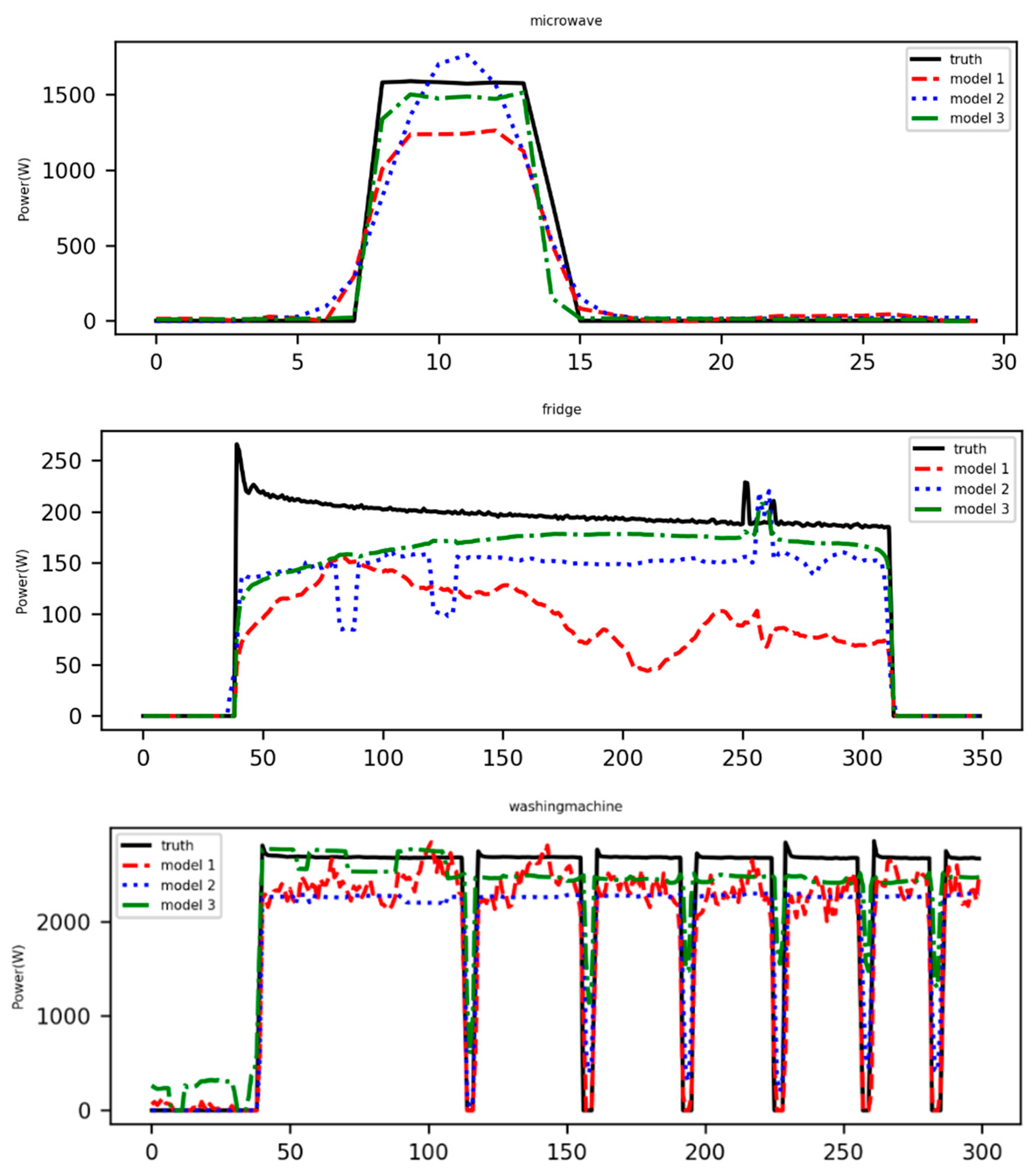
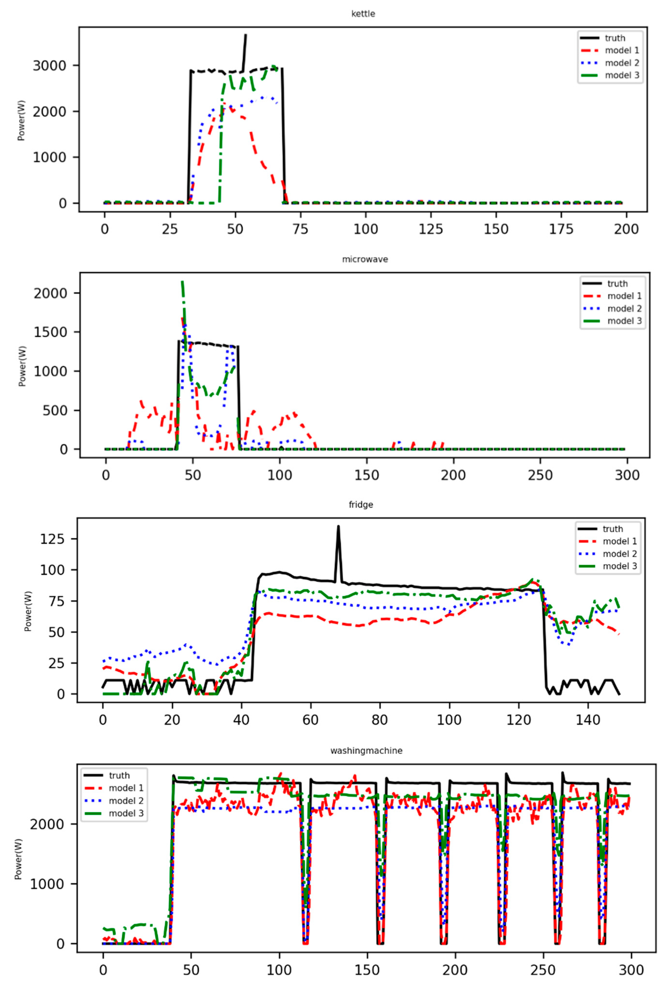
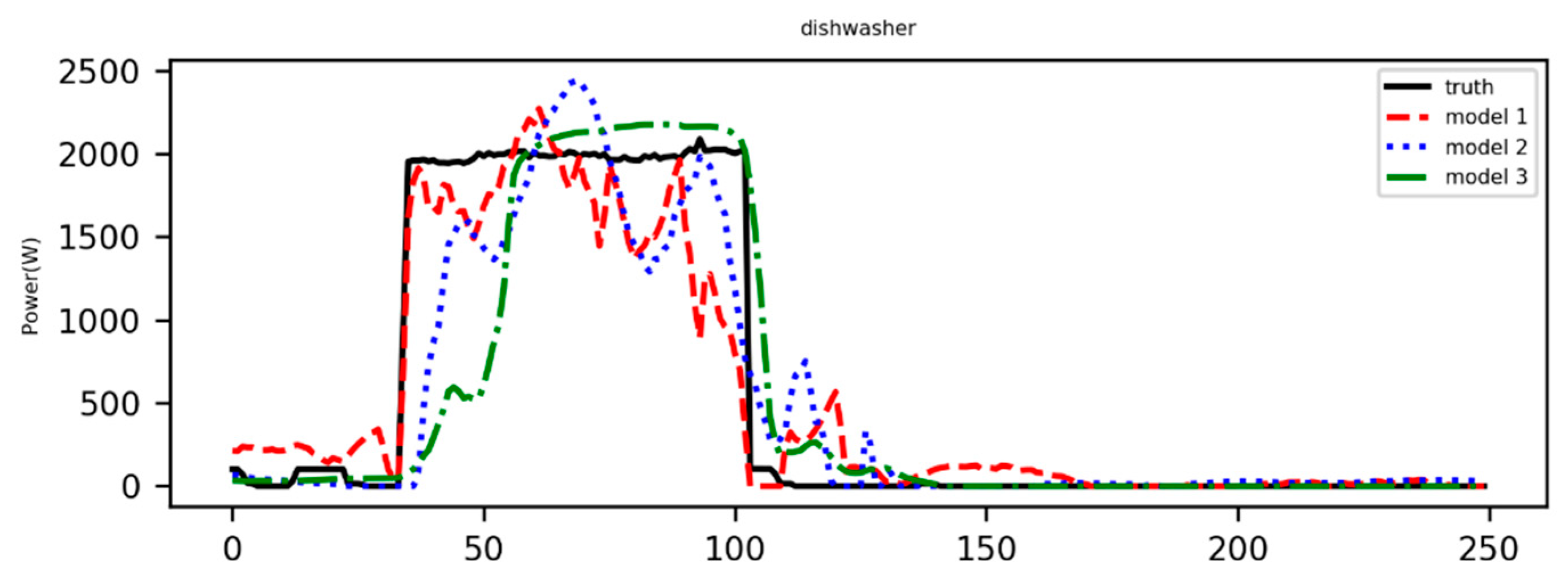
Figure 7 and Figure 8 show the decomposition results of the selected appliances from the testing house. The decomposition results of Model 3 are closer to the real values in most cases. The results show that the decomposition effect on the fridge was superior to that on the microwave or dishwasher. The possible explanation is the microwave has a short operation time and large power variations. When other appliances are running simultaneously, the superposition of the power signals increases the difficulty of load decomposition. In addition, the last picture in Figure 7 shows that the decomposition of the dishwasher is difficult during the change of working stages. Model 3 proposed in this study did much better than Model 1 in this case.
It should be noted that the results obtained in this experiment are not entirely consistent with Zhang’s paper, which may be due to some differences between the data processing and the selected hyper-parameters. For a fair comparison, regularization techniques, such as dropout, L1 and L2 regularizations, were not included. In addition, the hyper-parameters were not fine-tuned carefully. Therefore, there is still a risk of overfitting.

4.2. Comparison of the s2p and the s2s Model

In this study, we added another experiment to compare s2s and s2p learning methods. Model 4 represents the s2s+bahdanau attention+self-attention model, which is entirely consistent with Model 3, the s2p+bahdanau attention+self-attention model, except that the last dense layer outputs a sequence instead of a point. The output sequence’s length equals the input sequence, which indicates the power values of the target electrical appliance within a time window. Due to the sliding window technique used in this paper, the output sequences are overlapped each other, so it is necessary to average the overlapping parts as the predicted values at each time point. Model 4 was trained on House 1 and tested on House 2 in UK-DALE, and the training parameters were consistent with those of Model 3. The experimental results are compared in Figure 9. Model 3 is superior to Model 4, except for microwave on the SAE. The number of MAE decreased most on the microwave, by 24%, and decreased least on the washing machine, by 14%. On the SAE metric, Model 3 decreased the kettle, washing machine, fridge, dishwasher by 27%, 18%, 30%, and 25%, respectively. The numbers of MR were also significantly reduced on all five appliances. These experiment results support the conclusions drawn in [23]: s2p is better than s2s for NILM.

5. Conclusions

This study improves the sequence-to-point learning method via the attention mechanism in NILM. The attention mechanism has made remarkable progress in machine translation and other fields, so many researchers have recently adopted this technology to NILM. However, it is unclear how to combine attention mechanism with existing models because the attention mechanism has developed many different variants. Therefore, it is still a challenge to choose an appropriate model. In this study, two deep neural networks based on the attention mechanism were proposed for NILM. The models employ the Bahdanau style attention and self-attention mechanism to improve the s2p model. The experiment results on the public datasets REDD and UK-DALE show that in most cases, the new models have a better effect than s2p (Zhang) model. Model 3 employed with both bahdanau attention and self-attention performs best in most evaluation metrics and dramatically shortens the training time of Model 2. In the supplementary experiment, Model 3 outperforms Model 4, which indicates that the s2p model is superior to the s2s model in solving the NILM problem. Since the objective of this study was load decomposition rather than ED, only low-frequency active power data were used, as the previous studies referenced in this paper. However, multiple features should be included to improve the performance, such as reactive power, apparent power, current, and and voltage in future studies.
A few recent studies have applied different network structures to solve the NILM problem and claimed to have achieved a status of state-of-the-art [24,25,34]. However, most of them, e.g., [24,25], have not published their codes, so it is difficult to repeat their experimental results for comparison. Some studies use models other than s2s (s2p) learning, e.g., CNN [34], which is not the focus of this paper. Nevertheless, all the researches show that deep learning is a promising load decomposition technique. However, there are still many challenges that can be summarized in terms of two aspects: data and model. For this reason, we believe creating richer features and searching for the best network structure is worthy of future study. In addition, because the model training takes a long time, the utilization of the pre-trained model to perform transfer learning on a new dataset to shorten the training time should be considered.

Author Contributions

M.Y. conceived, designed, and performed the experiments; Y.L. and M.Y. wrote the paper; X.L. reviewed the paper and contributed experimental tools. All authors have read and agreed to the published version of the manuscript.

Funding

This work was supported by the National Natural Science Foundation of China, grant number 71473250.

Conflicts of Interest

The authors declare no conflict of interest.

References

  1. Hart, G.W. Nonintrusive Appliance Load Monitoring. Proc. IEEE 1992, 80, 1870–1891. [Google Scholar] [CrossRef]
  2. Gupta, S.; Reynolds, M.S.; Patel, S.N. ElectriSense: Single-Point Sensing Using EMI for Electrical Event Detection and Classification in the Home. In Proceedings of the 12th ACM International Conference on Ubiquitous Computing, Copenhagen, Denmark, 26–29 September 2010; pp. 139–148. [Google Scholar] [CrossRef]
  3. Bouhouras, A.S.; Milioudis, A.N.; Labridis, D.P. Development of Distinct Load Signatures for Higher Efficiency of NILM Algorithms. Electr. Power Syst. Res. 2014, 117, 163–171. [Google Scholar] [CrossRef]
  4. Matsui, K.; Yamagata, Y.; Nishi, H. Disaggregation of Electric Appliance’s Consumption Using Collected Data by Smart Metering System. Energy Procedia 2015, 75, 2940–2945. [Google Scholar] [CrossRef] [Green Version]
  5. Lin, S.; Zhao, L.; Li, F.; Liu, Q.; Li, D.; Fu, Y. A Nonintrusive Load Identification Method for Residential Applications Based on Quadratic Programming. Electr. Power Syst. Res. 2016, 133, 241–248. [Google Scholar] [CrossRef] [Green Version]
  6. Leeb, S.B.; Shaw, S.R.; Kirtley, J.L. Transient Event Detection in Spectral Envelope Estimates for Nonintrusive Load Monitoring. IEEE Trans. Power Deliv. 2014, 10, 1200–1210. [Google Scholar] [CrossRef] [Green Version]
  7. Xiang, C.; Linzhi, L.I.; Hao, W.U.; Yi, D.; Yonghua, S.; Weizhen, S.U.N.; Xiang, C.; Linzhi, L.I.; Hao, W.U.; Yi, D.; et al. A Survey of The Research on Non-intrusive Load Monitoring and Disaggregation. Power Syst. Technol. 2016, 40, 3108–3117. [Google Scholar] [CrossRef]
  8. Dong, M.; Meira, P.C.M.; Xu, W.; Chung, C.Y. Non-Intrusive Signature Extraction for Major Residential Loads. IEEE Trans. Smart Grid 2013, 4, 1421–1430. [Google Scholar] [CrossRef] [Green Version]
  9. Faustine, A.; Mvungi, N.H.; Kaijage, S.; Michael, K. A Survey on Non-Intrusive Load Monitoring Methodies and Techniques for Energy Disaggregation Problem. arXiv 2017, arXiv:1703.00785. Available online: http://arxiv.org/abs/1703.00785 (accessed on 10 March 2017).
  10. Ruano, A.; Hernandez, A.; Ureña, J.; Ruano, M.; Garcia, J. NILM Techniques for Intelligent Home Energy Management and Ambient Assisted Living: A Review. Energies 2019, 12, 2203. [Google Scholar] [CrossRef] [Green Version]
  11. Huber, P.; Calatroni, A.; Rumsch, A.; Paice, A. Review on Deep Neural Networks Applied to Low-Frequency NILM. Energies 2021, 14, 2390. [Google Scholar] [CrossRef]
  12. Uribe-Pérez, N.; Hernández, L.; De la Vega, D.; Angulo, I. State of the Art and Trends Review of Smart Metering in Electricity Grids. Appl. Sci. 2016, 6, 68. [Google Scholar] [CrossRef]
  13. Pereira, L.; Nunes, N. An Experimental Comparison of Performance Metrics for Event Detection Algorithms in NILM. In Proceedings of the 4th International NILM Workshop, Austin, TX, USA, 7 March 2018. [Google Scholar]
  14. Athanasiadis, C.; Doukas, D.; Papadopoulos, T.; Chrysopoulos, A. A Scalable Real-Time Non-Intrusive Load Monitoring System for the Estimation of Household Appliance Power Consumption. Energies 2021, 14, 767. [Google Scholar] [CrossRef]
  15. Kelly, J.; Knottenbelt, W. Neural NILM:Deep Neural Networks Applied to Energy Disaggregation. In Proceedings of the ACM International Conference on Embedded Systems for Energy-Efficient Built Environments, Seoul, Korea, 4 November 2015; pp. 55–64. [Google Scholar]
  16. Kelly, J.; Knottenbelt, W. The UK-DALE Dataset, Domestic Appliance-Level Electricity Demand and Whole-House Demand from Five UK Homes. Sci. Data 2015, 2, 1–14. [Google Scholar] [CrossRef] [Green Version]
  17. Medeiros, A.P.; Canha, L.N.; Bertineti, D.P.; de Azevedo, R.M. Event Classification in Non-Intrusive Load Monitoring Using Convolutional Neural Network. In Proceedings of the 2019 IEEE PES Innovative Smart Grid Technologies Conference—Latin America (ISGT Latin America), Gramado, Brazil, 15–18 September 2019; pp. 1–6. [Google Scholar]
  18. Çavdar, İ.H.; Faryad, V. New Design of a Supervised Energy Disaggregation Model Based on the Deep Neural Network for a Smart Grid. Energies 2019, 12, 1217. [Google Scholar] [CrossRef] [Green Version]
  19. Balduzzi, D.; Frean, M.; Leary, L.; Lewis, J.P.; Ma, K.W.-D.; McWilliams, B. The Shattered Gradients Problem: If Resnets Are the Answer, Then What Is the Question? arXiv 2018, arXiv:1702.08591. [Google Scholar]
  20. Jiang, J.; Kong, Q.; Plumbley, M.; Gilbert, N. Deep Learning Based Energy Disaggregation and On/Off Detection of Household Appliances. arXiv 2019, arXiv:1908.00941. [Google Scholar]
  21. Sutskever, I.; Vinyals, O.; Le, Q.V. Sequence to Sequence Learning with Neural Networks. In Proceedings of the Advances in Neural Information Processing Systems, Montreal, QC, Canada, 8–13 December 2014; pp. 3104–3112. [Google Scholar]
  22. Xia, M.; Liu, W.; Wang, K.; Zhang, X.; Xu, Y. Non-Intrusive Load Disaggregation Based on Deep Dilated Residual Network. Electr. Power Syst. Res. 2019, 170, 277–285. [Google Scholar] [CrossRef]
  23. Zhang, C.; Zhong, M.; Wang, Z.; Goddard, N.; Sutton, C. Sequence-to-Point Learning with Neural Networks for Nonintrusive Load Monitoring. arXiv 2017, arXiv:1612.09106. [Google Scholar]
  24. Jia, Z.; Yang, L.; Zhang, Z.; Liu, H.; Kong, F. Sequence to Point Learning Based on Bidirectional Dilated Residual Network for Non-Intrusive Load Monitoring. Int. J. Electr. Power Energy Syst. 2021, 129, 106837. [Google Scholar] [CrossRef]
  25. Sudoso, A.M.; Piccialli, V. Non-Intrusive Load Monitoring with an Attention-Based Deep Neural Network. arXiv 2019, arXiv:1912.00759. [Google Scholar]
  26. Bahdanau, D.; Cho, K.; Bengio, Y. Neural Machine Translation by Jointly Learning to Align and Translate. arXiv 2014, arXiv:1409.0473. [Google Scholar]
  27. Vaswani, A.; Shazeer, N.; Parmar, N.; Uszkoreit, J.; Jones, L.; Gomez, A.N.; Kaiser, L.; Polosukhin, I. Attention Is All You Need. arXiv 2017, arXiv:1706.03762. [Google Scholar]
  28. Kolter, J.Z.; Jaakkola, T. Approximate Inference in Additive Factorial HMMs with Application to Energy Disaggregation. In Proceedings of the Fifteenth International Conference on Artificial Intelligence and Statistics, Palma, Canary Islands, 21–23 April 2012; Volume 22, pp. 1472–1482. [Google Scholar]
  29. Kazemi, S.M.; Goel, R.; Eghbali, S.; Ramanan, J.; Sahota, J.; Thakur, S.; Wu, S.; Smyth, C.; Poupart, P.; Brubaker, M. Time2Vec: Learning a Vector Representation of Time. arXiv 2019, arXiv:1907.05321. [Google Scholar]
  30. Kolter, J.Z.; Johnson, M.J. REDD: A Public Data Set for Energy Disaggregation Research. In Proceedings of the Workshop on Data Mining Applications in Sustainability (SIGKDD), San Diego, CA, USA, 21 August 2011; Volume 25, pp. 59–62. [Google Scholar]
  31. Batra, N.; Kelly, J.; Parson, O.; Dutta, H.; Knottenbelt, W.; Rogers, A.; Singh, A.; Srivastava, M. NILMTK: An Open Source Toolkit for Non-Intrusive Load Monitoring. In Proceedings of the 5th International Conference on Future Energy Systems, Cambridge, UK, 11–13 June 2014; pp. 265–276. [Google Scholar] [CrossRef] [Green Version]
  32. Batra, N.; Kukunuri, R.; Pandey, A.; Malakar, R.; Kumar, R.; Krystalakos, O.; Zhong, M.; Meira, P.; Parson, O. A Demonstration of Reproducible State-of-the-Art Energy Disaggregation Using NILMTK. In Proceedings of the 6th ACM International Conference on Systems for Energy-Efficient Buildings, Cities, and Transportation, Association for Computing Machinery, New York, NY, USA, 13 November 2019; pp. 358–359. [Google Scholar]
  33. Mayhorn, E.T.; Sullivan, G.P.; Petersen, J.M.; Butner, R.S.; Johnson, E.M. Load Disaggregation Technologies: Real World and Laboratory Performance; Pacific Northwest National Lab. (PNNL): Richland, WA, USA, 2016. [Google Scholar]
  34. Chen, K.; Zhang, Y.; Wang, Q.; Hu, J.; Fan, H.; He, J. Scale-and Context-Aware Convolutional Non-Intrusive Load Monitoring. IEEE Trans. Power Syst. 2019, 35, 2362–2373. [Google Scholar] [CrossRef] [Green Version]
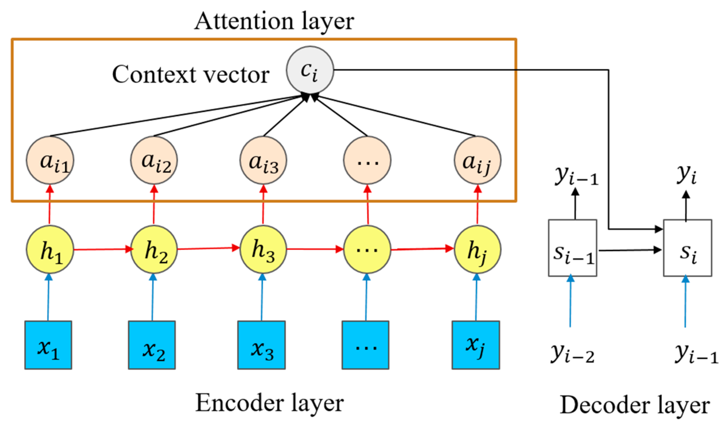
Figure 1. Bahdanau attention mechanism.
Electronics 10 01657 g001
Figure 2. Self-attention mechanism.
Electronics 10 01657 g002
Figure 3. Network structure of s2p (Zhang) model.
Electronics 10 01657 g003
Figure 4. Network structure of s2p+bahdanau attention model.
Electronics 10 01657 g004
Figure 5. Network structure of s2p+bahdanau attention+self-attention model.
Electronics 10 01657 g005
Figure 6. Modified bahdanau attention mechanism.
Electronics 10 01657 g006
Figure 7. The decomposition results on REDD (timestep 6 s).
Electronics 10 01657 g007aElectronics 10 01657 g007b
Figure 8. The decomposition results on UK-DALE (timestep 6 s).
Electronics 10 01657 g008aElectronics 10 01657 g008b
Figure 9. Comparison of metrics between s2s and s2p learning method on UK-DALE. (a) MAE, (b) SAE, (c) MR.
Electronics 10 01657 g009
Table 1. Parameters for Normalizing.
ParameterMeanStd
Aggregate522814
Kettle7001000
Microwave500800
Refrigerator200400
Dishwasher7001000
Washing machine400700
Table 2. Hyperparameters for Training.
Input Window Length599
Maximum Epochs100
Batch Size1000
Patience of Early-Stopping5
Learning Rate0.001
Table 3. Total parameters and one epoch training time for three models.
ModelTotal ParametersTraining Time (1.2 M Samples)
Model 130,708,249249 s
Model 21,359,174535 s
Model 3953,643229 s
Table 4. Evaluation results on REDD.
MetricsModelMicrowave Washing MachineFridgeDishwasher
MAEModel 125.2637.4032.6619.44
Model 219.4441.5215.7718.67
Model 315.3322.3724.4315.73
SAEModel 10.240.490.280.32
Model 20.160.310.180.66
Model 30.120.230.110.29
MRModel 10.220.210.480.17
Model 20.330.340.650.21
Model 30.150.170.310.14
Table 5. Evaluation results on UK-DALE.
MetricsModelKettleMicrowaveWashing MachineFridgeDishwasher
MAEModel 112.2214.6225.0325.1837.12
Model 211.4413.6223.1522.8247.47
Model37.357.7415.1217.3338.66
SAEModel 10.140.480.280.150.32
Model 20.210.500.310.110.35
Model 30.080.310.180.090.24
MRModel 10.240.510.330.270.46
Model 20.180.440.280.210.33
Model 30.110.410.190.140.44
Publisher’s Note: MDPI stays neutral with regard to jurisdictional claims in published maps and institutional affiliations.