Design of a High-Power High-Efficiency Multi-Receiver Wireless Power Transfer System

Abstract

This paper proposes a new control method to regulate the power flow into multiple receivers. This system consists of one transmitter controller and three receiver controllers. They work independently to decide the power distribution with their combined operation. The simulated and experimental models have been built, and the experimental results are in good agreement with the theoretical analysis results. The proposed method is robust, flexible, and generalizable, and can be employed under various wireless charging conditions.

1. Introduction

Wireless power transfer (WPT) is a technology that enables power transfer in a convenient and safe manner without any physical contact. WPT is widely used in many areas, such as cell phones, household appliances, industrial robots, and electric vehicles. There are many WPT system that can charge multiple receivers with a single transmitter. Tightly coupled inductive technology based on wireless power consortium (WPC or Qi) or loosely coupled magnetic resonant technology based on air fuel has been widely used in multi-receiver WPT systems, where receivers are powered simultaneously.

Many literatures have investigated various aspects regarding multi-receiver WPT systems, such as efficiency optimization [1,2,3,4,5], multi-frequency WPT [6], transfer characteristics [7,8], energy encryption [9], omnidirectional WPT [10], cross coupling effect [11,12], reconfigurable WPT [13], and bidirectional power transfer [14]. To extend the application scope of multi-receiver WPT, the system should be more generalizable and robust with flexible receiver number and power levels.

However, there are some challenges with the power distribution of multi-receiver WPT systems. First, receivers close to the transmitter tend to absorb more power than the ones far away [15], whereas the power demand of each receiver should be decided by its load instead of receiver distance. Second, many factors, such as power demand, receiver distances and receiver number may dynamically change. Third, the power capacity of the transmitter becomes more insufficient to meet the demands with the increase in receiver number. In most cases, the peak power demand is much higher than the average power demand [16]. Therefore, the transmitter may be overloaded if the receivers absorb more power than the capacity of the transmitter.

Recently, some methods have been proposed to control the power distribution in multi-receiver WPT systems. In [16], the frequency is used as the communication channel for the entire system. Receivers are configured to different priority levels. When the transmitter is on the verge of overloading, the power of all the receivers is decreased simultaneously. Reference [17] proposes a power distribution scheme that can be adapted to the variations in the load parameters. This scheme employs an impedance regulator at the receiver side to match the power demand of the loads. A transmitter controller is used to alter a capacitor array to control the total equivalent impedance. Reference [18] adopts a time-sharing method, which selectively and exclusively delivers power to only one designated receiver among multiple receivers. The power division ratio is controlled by changing the duration time ratio for power transfer. This method is realized by separating the resonant frequency of every receiver. In [19], multiple frequencies are tuned into one transmitting coil with multiple inverters. Receivers are tuned at different corresponding frequencies; thus, the power transferred to each receiver can be controlled independently. However, this configuration is complex and costly. Reference [15] proposes a method to control the power division ratio through an impedance matching circuit. However, the power division ratio is sensitive to the coupling coefficient, frequency, and load resistance, making this method less flexible. References [4,20] have designed the power division ratio by adjusting the load impedance. However, the load impedance cannot be changed in some practical WPT systems. Reference [21] proposed a game-theory-based power distribution control method, whereby the charging power distribution is determined and updated through the interplay between the existing receivers.

Although several different types of power distribution approaches have proposed in aforementioned literature, these solutions still cannot satisfy all the requirements of large-scale application, such as power demand of each receiver, transmitter overloading prevention, equivalent impedance matching, flexible power ratio, easy configuration, and compact size. Some methods are costly and complicated in hardware and software implementation. In addition, some methods have limitations in the number of receivers.

To improve performance and overcome some limitations of the existing methods, this paper has proposed a new power distribution method for multi-receiver WPT system. This method introduces competition mechanism to distribute power, which can achieve dynamic power distribution. The proposed method is simple in both hardware and software implementation with no limit in the number of receivers.

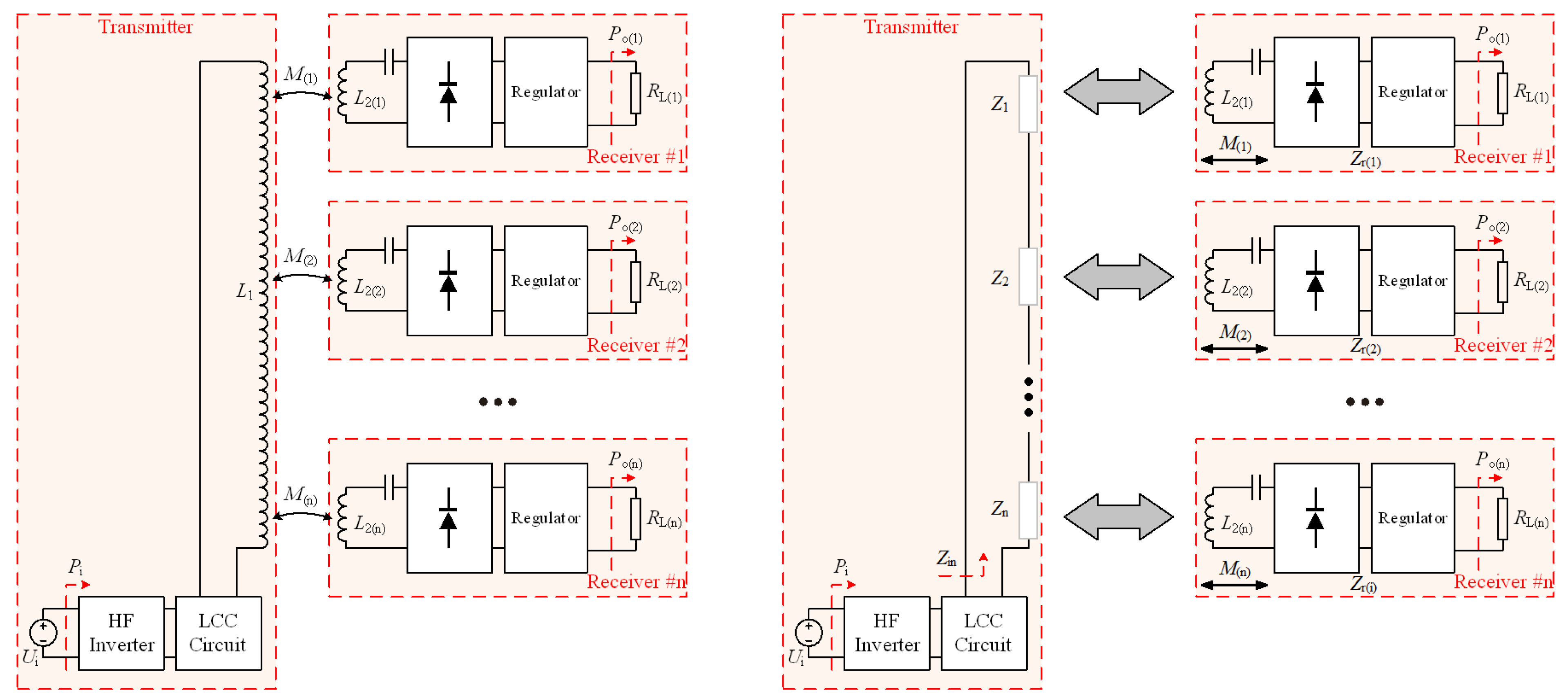
2. Multi-Receiver WPT Systems

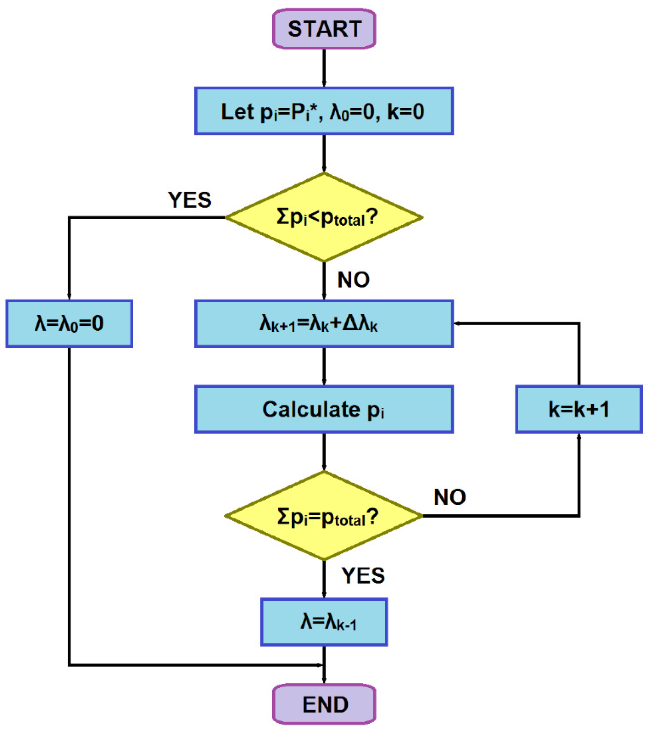
2.1. Competition Theory Analysis

A typical multi-receiver WPT system is shown in Figure 1. The transmitter is powered by a DC power supply. The current in the transmitting coil produces magnetic field around the transmitting coil, voltage is induced in all receiving coils, and then power will be delivered to all receivers simultaneously. When a receiver needs more power, the transmitter sees impedance changes. Since all receiver coils are parallel, the cross-coupling can usually be neglected [22,23], the reflected impedance Z_i can be derived as [23].

$$Z_i=\frac{{\omega }^2{M}_{\left(i\right)}^2}{Z_{r\left(i\right)}+R_{L\left(i\right)}}$$

(1)

where ω is the operating angular frequency; M_(i) is the mutual inductance between the TX coil and the i-th RX coil; Z_ri is the equivalent impedance seen though RX. Under resonance condition, the load impedance seen by the input is

$$Z_{in}={\displaystyle \sum _{i=1}^n{Z}_i}$$

(2)

The output power from the input is first transferred to the i-th RX coil, and then to the load. Then, the power received by the i-th load can be calculated to be

$$P_{o\left(i\right)}=P_i\frac{\mathrm{Re}\left\{Z_i\right\}}{{\displaystyle {\sum }_{i=1}^n\mathrm{Re}\left\{Z_i\right\}}}\cdot \frac{R_{L\left(i\right)}}{\mathrm{Re}\left\{Z_{r\left(i\right)}\right\}+R_{L\left(i\right)}}$$

(3)

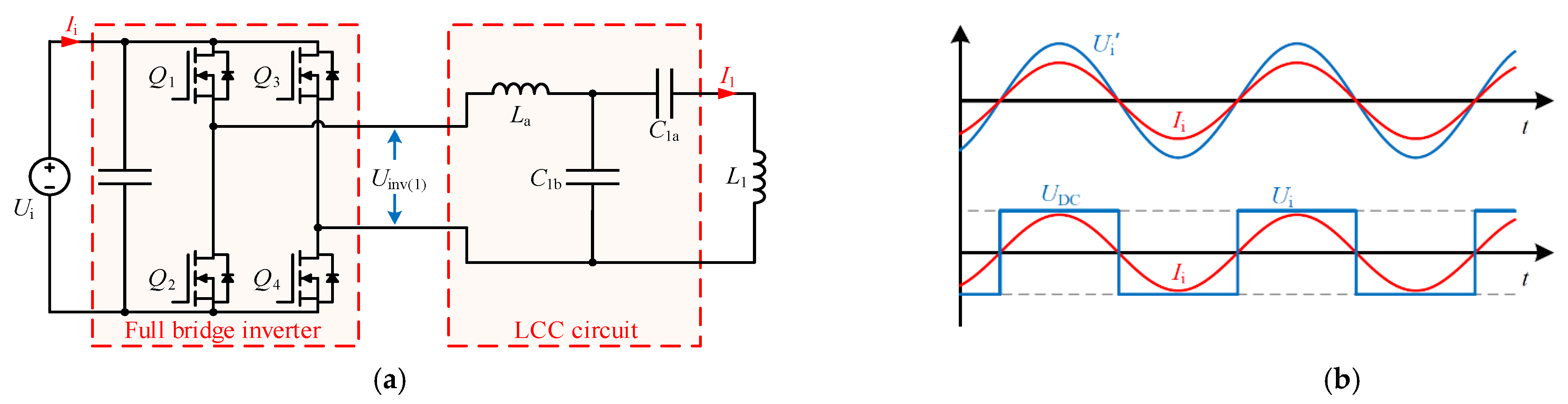
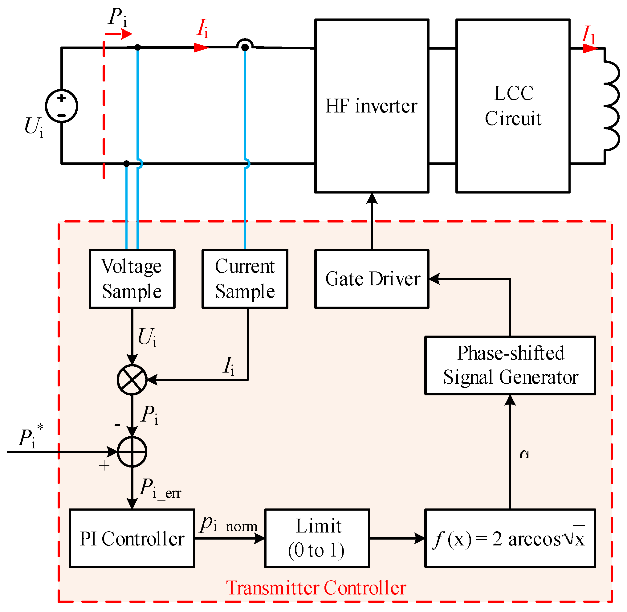
2.2. Transmitter Analysis

The schematic of the transmitter is shown in Figure 2. A high-frequency (HF) inverter converts the DC power to HF AC power, and then the power is driven into the transmitting compensation circuit through the coils.

The inverter adopts a full bridge configuration, and the amplitude of its output is controlled by phase-shift angle α. The waveform of inverter output voltage U_inv is a square waveform which consists of an infinite number of harmonics. When the rms of the fundamental component of U_inv (which is defined as U_inv(1)) is considered, the relationship between U_inv(1) and phase-shift angle α is

$$U_{inv(1)}=\frac{2\sqrt{2}}{\pi }\cos \left(\frac{\alpha }{2}\right)U_i$$

(4)

The LCC circuit is employed for the transmitter as the compensation circuit, which consists of three components L_a, C_1a, and C_1b. The matching condition of the LCC circuit is [5]:

$$\omega L_a=\frac{1}{\omega C_{1b}}=\omega L_1-\frac{1}{\omega C_{1a}}$$

(5)

where ω is the angular frequency and L₁ is the self-inductance of transmitting coil. Then, the rms value of transmitting coil current I₁ is [24]:

$$I_1=\frac{U_{inv(1)}}{\omega L_a}$$

(6)

The transmitting coil current is proportional to U_inv(1), irrespective of the load impedance. Compared with other common compensation circuits such as series compensation circuit, LCC compensation circuit has advantage of constant current characteristics, which is helpful to decouple receivers. The duty cycle is controlled under constant frequency and it is done easily.

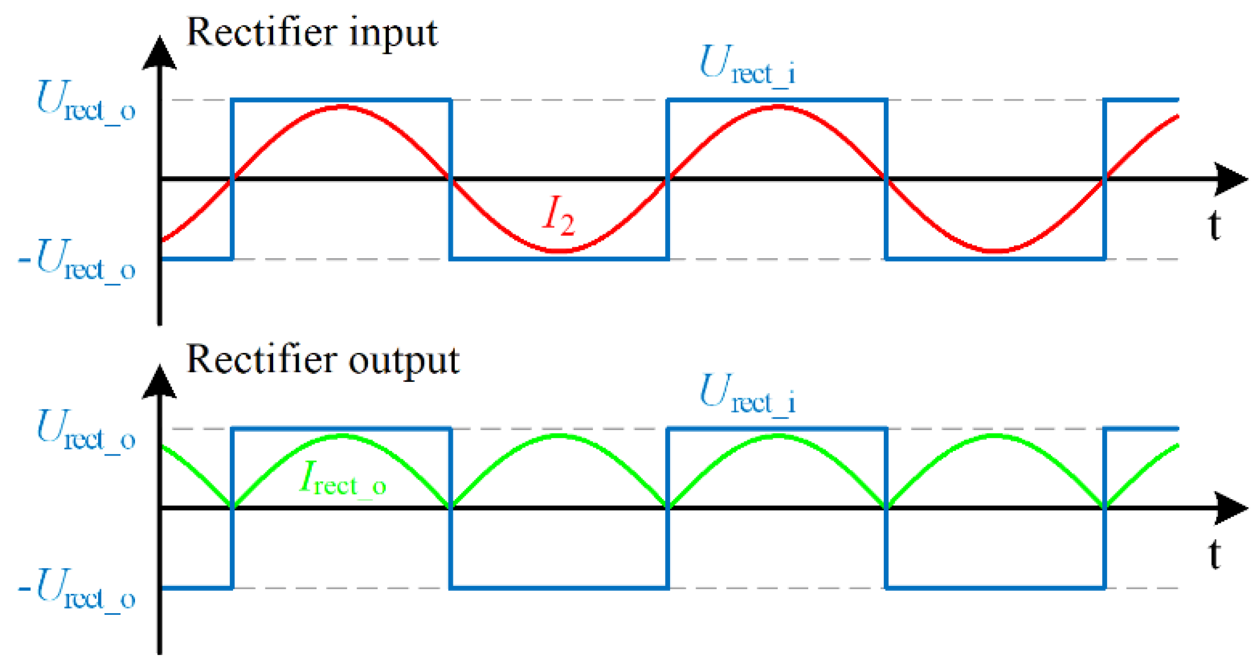
2.3. Receiver Analysis

The receiver consists of a receiving coil, a compensation circuit, a rectifier, and a regulator, as shown in Figure 3. The induced voltage U₂ in receiving coil can be regarded as a voltage source in series with receiver coil, and its rms value can be calculated as:

$$U_2=\omega M{I}_1$$

(7)

The input current of the rectifier I₂ is distorted because of the non-linear characteristics of the rectifier. The average power supplied by U₂ is:

$$P_2=U_2{I}_2$$

(8)

The rectifier input waveform is shown in Figure 4. The output current of the rectifier can be expressed using Fourier harmonic expansion as [25].

$$I_{rect\_o}=\sqrt{2}{I}_2\left(\frac{2}{\pi }-\frac{4}{3\pi }\cos 2\omega t-\frac{4}{15\pi }\cos 4\omega t-\frac{4}{35\pi }\cos 6\omega t\dots \right)$$

(9)

Then, the input power of rectifier P_{rect_i} can be derived using sinusoidal trigonometric functions calculus [26]. Since the power is calculated within a time period, only the DC term is not zero and P_{rect_i} can be calculated to be:

$$P_{ret\_i}=\frac{1}{T}{\displaystyle {\int }_0^T{U}_{rect\_o}{I}_{rect\_o}=}\frac{2\sqrt{2}}{\pi }{U}_{rect\_o}{I}_2$$

(10)

where U_{rect_o} is the rectifier output voltage. The power losses of the rectifier is very small and, therefore, can be neglected, and the average power supply can be calculated as:

$$P_2\approx P_{rect\_i}$$

(11)

The relationship between U₂ and U_{rect_o} can be derived from (10):

$$U_{rect\_o}=\frac{\pi }{2\sqrt{2}}{U}_2$$

(12)

The regulator is a half-bridge converter, and its output voltage U_o is

$$U_o=D{U}_{rect\_o}$$

(13)

where D is the duty cycle of the regulator.

By combining (4), (6), (11), (12) and (13), the output power to the load P_o can be derived as:

$$P_o=\frac{U_o^2}{R_L}=\frac{{\left(M{U}_{i}D\cos \frac{\alpha }{2}\right)}^2}{R_L{L}_a^2}$$

(14)

It can be noted from (14) that P_o can be controlled by α and D.

In our multi-receiver WPT system, the transmitting LCC circuit could minimize the effect of cross coupling due to its constant current characteristic of the transmitting coil [20]. The output power satisfies (14) and can be rewritten as a function of the control variable α and duty cycle of the ith regulator D_(i):

$$P_{o\left(i\right)}=f\left(\alpha ,D_{\left(i\right)}\right)=\frac{{\left(U_i\cos \frac{\alpha }{2}\right)}^2}{L_a^2}\times \frac{{\left(M_{\left(i\right)}{D}_{\left(i\right)}\right)}^2}{R_{L\left(i\right)}}$$

(15)

where M_(i) is the mutual inductance between the transmitting coil and the coil of receiver #i, R_L(i) is the load resistance of receiver #i. P_o(i) can be regulated by the two parameters indicated in (15):α and D_(i). In a single receiver WPT system, only one parameter needs to be changed to achieve desired power regulation, with the other one fixed.

The total output power of the receivers P_{o_sum} can be expressed as follows:

$$P_{o_{-}sum}={\displaystyle \sum _{i=1}^n{P}_{o(i)}}=\frac{{\left(U_i\cos \frac{\alpha }{2}\right)}^2}{L_a^2}\times {\displaystyle \sum _{i=1}^n\frac{{\left(M_{(i)}{D}_{(i)}\right)}^2}{R_{L(i)}}}$$

(16)

where n is the number of receivers.

The efficiency of the entire system η is defined as:

$$\eta =\frac{P_{o\_sum}}{P_i}$$

(17)

where P_i is the input power of transmitter, which can be derived as:

$$P_i=\frac{P_{o_{-}sum}}{\eta }=\frac{{(U_i\cos \frac{\alpha }{2})}^2}{\eta L_a^2}\times {\displaystyle \sum _{i=1}^n\frac{{\left(M_{(i)}{D}_{(i)}\right)}^2}{R_{L(i)}}}$$

(18)

For a multi-receiver WPT system, the power distribution control strategy should satisfy two basic principles. First, the transmitter has limited power capacity, and it should not overload at any given time. Second, the power demand by each receiver should be satisfied as much as possible. When the power capacity of the transmitter meets the demand of all the receivers, every receiver should receive the required amount of power. When the power capacity of transmitter is lower than the total power demand of the receivers, and receivers should absorb less power than their demands to prevent overloading.

2.4. The Proposed Structure Analysis

Our proposed structure employs double-side control and it is comprised of two types of controllers. The first type is the transmitter controller. There is only one transmitter controller in the multi-receiver WPT system, and it is located at the transmitting side to regulate the total power of the WPT system and to prevent overloading the DC power supply. The second type is the receiver controller. Every receiver has an individual receiver controller. Based on the circuit topology, the system provides adaptive output based on the load requirement in each receiver. The current in the transmitting coil produces magnetic field around the transmitting coil, and voltage is induced in all receiving coils, and then power is delivered to all receivers simultaneously. The regulators control the output power of each load are based on the design requirements. Power distribution comes from mutual inductions and actual DCs loads.

The structure of the proposed transmitter controller is shown in Figure 5. This system contains a feedback loop with a PI controller and phase-shifted signal generator. The voltage and current values are sampled in to calculate the input power P_i. This value is subtracted with the instructed power value P_i* to obtain the error power P_{i_err}. Then the error power is normalized in the domain (0, 1) to feedback the phase-shifted signal generator, which controls the gate driver of the HF invertor. Additional anti-trigonometric square root function is integrated to increase the stability and robustness of the controller.

The transmitter controller would control the power of the entire system such that the instruction input power is not exceeded. The instruction input power is set to be slightly lower than the power capacity of the DC power supply to preserve redundancy power of the supply. First, the input voltage and input current of the inverter are sampled through a sampling circuit, and the input power of the inverter is measured by multiplying the input voltage and t current. The error between the instructed and measured power is calculated through subtraction. A proportional–integral (PI) controller then regulates the input power of the inverter based on the input error.

It can be seen from (18) that the DC power supply has the maximum output power P_{i_max} when the inverter phase shift angle α is equal to 0, that is:

$$P_{i\_max}={P_i|}_{\alpha =0^{°}}=\frac{U_i^2}{\eta L_a^2}\times {\displaystyle \sum _{i=1}^n\frac{{\left(M_{(i)}{D}_{(i)}\right)}^2}{R_{L(i)}}}$$

(19)

The output of the PI controller represents the normalized power p_{i_norm}, which is the ratio of the P_i to P_{i_max}. Combining (18) and (19), p_{i_norm} can be derived as:

$$p_{i_{-}norm}=\frac{P_i}{P_{i_{-}max}}={\cos }^2\left(\frac{\alpha }{2}\right)$$

(20)

Since p_{i_norm} is between 0 and 1, the output of the PI controller is limited from 0 to 1. By rewriting (20), the phase shift angle of the inverter α can be derived as:

$$\alpha =2\arccos \sqrt{p_{i_{-}norm}}$$

(21)

Therefore, a math function block is inserted after the PI controller to calculate the phase shift angle α. Finally, a phase-shifted signal generator produces the control signal for the inverter, and the gate driver drives the semiconductor switches in the inverter.

The transmitter controller regulates the inverter input power to prevent overloading of the DC power supply. Two possible states may appear for the transmitter controller. In state 1, P_i* is less than P_{i_max}, while in state 2, the instruction input power P_i* is greater than or equal to P_{i_max}, as shown in Figure 6.

State 1: P_i* < P_{i_max}. Considering a scenario at time t₀, P_i is greater than P_i*, the error power P_{i_err} is negative, the PI controller decreases P_{i_norm}, α increase, and, therefore, P_i decreases. On the contrary, if P_i is less than P_i* at t₀, P_{i_err} would be positive, and the PI controller would increase P_{i_norm}, and α would decrease, and therefore P_i would be increased. The PI controller would adjust its output only if P_i is not equal to P_i*. Finally, in state 1, P_i will be equal to P_i* in the steady state. Moreover, there is no static error due to the integral part in the PI controller.

State 2: P_i* ≥ P_{i_max}. If P_i is less than P_{i_max} at time t₀, then P_i must also be less than P_i*. Similar to state 1, P_{i_err} is positive, and the PI controller would try to increase P_{i_norm} to increase P_i. When P_{i_norm} increases to 1 at t₁, P_i is equal to P_{i_max} but still less than P_i*. Therefore, the PI controller tends to continue to increase P_{i_norm}. However, P_{i_norm} is limited to be no greater than 1, so the P_{i_norm} would remain equal to 1, then the transmitter controller is saturated. Finally, in the steady state, P_i will be equal to P_{i_max} and would not increase to P_i*.

In summary, under steady state, P_i is always less than P_i* and P_{i_max} under the control of the transmitter controller, and can be calculated as

$$P_{i\_max}={P_i|}_{\alpha =0^{°}}=\frac{U_i^2}{\eta L_a^2}\times {\displaystyle \sum _{i=1}^n\frac{{\left(M_{(i)}{D}_{(i)}\right)}^2}{R_{L(i)}}}$$

(22)

Each receiver has an individual receiver controller to regulate its output for the load. This receiver controller is designed for constant-voltage output. The structure of the receiver controller is shown in Figure 7. The input to the receiver controller is the instructed output voltage ${U_{\left(o\right)i}}^{*}$. The output voltage U_o(i) is sampled through the sampling circuit. The error between ${U_{\left(o\right)i}}^{*}$ and U_o(i) is fed into the PI controller, and the output of which is the duty cycle D_(i) for the regulator. D_(i) is limited between 0 and 1. The PWM generator would generate the PWM control signal for the regulator, and the semiconductor switches are driven by the gate driver. Noting that once the instructed output voltage ${U_{\left(o\right)i}}^{*}$ is determined, the equivalent instruction output power P_o(i)* can be determined by:

$$P_{o(i)}^{*}=\frac{U_{o(i)}^{*}{}^2}{R_{L(i)}}=\frac{{\left(D^{*}{U}_{rect\_o}^{*}\right)}^2}{R_{L\left(i\right)}}$$

(23)

It can be seen that when duty cycle D_(i) equals to 1, the receiver has the maximum power:

$$P_{o{(i)}_{-}max}={P_{o(i)}|}_{D_{(i)}=1}=p_{i_{-}norm}\times \frac{{\left(M_{(i)}{U}_o\right)}^2}{R_{L(i)}{L}_a^2}={\cos }^2\left(\frac{\alpha }{2}\right)\times \frac{{\left(M_{(i)}D{U}_{rect\_o}\right)}^2}{R_{L(i)}{L}_a^2}$$

(24)

Similar to the transmitter controller, each receiver controller has two states:

State 1: ${U_{\left(o\right)i}}^{*}$ < U_{o(i)_max}. Figure 8a shows how the receiver controller regulates the output voltage in state 1. If U_o(i) is less than $U_{\left(o\right)i}^{*}$ at t₀, the error of the output voltage U_{o(i)_err} would be positive, and, then, the PI controller would increase the duty cycle D to increase U_o(i). On the contrary, if U_o(i) is higher than ${U_{\left(o\right)i}}^{*}$ at t₀, the error of the output voltage U_{o(i)_err} would be negative, so the PI controller would decrease the duty cycle D_(i) to decrease U_o(i). Finally, in the steady state, U_o(i) will be equal to ${U_{\left(o\right)i}}^{*}$ under the control of the receiver controller in state 1.

State 2: ${U_{\left(o\right)i}}^{*}$ ≥ U_{o(i)_max}. Figure 8b shows how the receiver controller works in state 2. If U_o(i) is less than U_{o(i)_max} at t₀, U_{o(i)_err} will be positive, and the PI controller would try to increase D_(i). When D_(i) increases to 1 at t₁, the output voltage will be U_{o(i)_max} while the output power is P_{o(i)_max}. U_{o(i)_err} would still remain positive. However, D_(i) is limited to be no greater than 1. Thus, the output voltage will no longer increase, which means that the receiver controller is saturated. Finally, in the steady state, the output voltage will remain U_{o(i)_max} in state 2.

In general, under the control of the receiver controller, the output voltage of the receiver in the steady state can be described as:

$$U_{o(i)}=\min \left(U_{o(i)}^{*},U_{o{(i)}_{-}max}\right)=\min \left(D^{*}{U}_{rect\_o}^{*},U_{o{(i)}_{-}max}\right)$$

(25)

The controllers at the transmitter and receiver sides regulate the power in their own ways. The operation principles of the transmitter and receiver controllers are relatively simple. However, the interaction between controllers is more important.

It is shown that P_{o(i)_max} varies with P_{i_norm}. However, P_{i_norm} is controlled by the transmitter controller. Thus, the regulation of the transmitter controller will change P_{o(i)_max}. The output power of a receiver is:

$$P_{o(i)}=P_{o{(i)}_{-}max}\times D_{(i)}^2$$

(26)

when P_{o(i)_max} is changed by the transmitter controller, the receiver controller will try to maintain the output voltage, as well as the output power by adjusting D_(i). Therefore, the transmitter controller will interfere with the receiver controllers.

Similarly, P_{i_max} varies with D in each receiver. Although D is controlled by the receiver controllers, the regulation of the receiver controllers will change P_{i_max}. For the transmitter, the power absorbed from the DC power supply is:

$$P_i=P_{i_{-}max}\times p_{i_{-}norm}=P_{i\_max}\times {\cos }^2\left(\frac{\alpha }{2}\right)$$

(27)

The transmitter will try to maintain P_i by adjusting P_{i_norm} when any receiver controller changes P_{i_max}. Therefore, the receiver controllers will also interfere with the transmitter controller.

Both the transmitter and receiver controllers will participate in the regulation process before the system enters the steady state, with the two types of controllers affecting each other during the regulation. The power distribution is the result of the interaction between the controllers.

The following relationship is derived by combining (16) and (17):

$${\displaystyle \sum _{i=1}^n{P}_{o(i)}}=\eta P_i$$

(28)

From (20), the ratio of P_{o_max} between the receivers can be calculated as:

$$P_{o{(i)}_{-}max}:P_{o{(j)}_{-}max}=p_{i\_norm}\times \frac{{\left(M_{\left(i\right)}{U}_o\right)}^2}{R_{L\left(i\right)}{L}_a^2}:p_{i\_norm}\times \frac{{\left(M_{\left(j\right)}{U}_o\right)}^2}{R_{L\left(j\right)}{L}_a^2}=\frac{M_{(i)}^2}{R_{L(i)}}:\frac{M_{(j)}^2}{R_{L(j)}}$$

(29)

where i and j are the serial numbers of receivers.

Under the assumption that the efficiency is constant and by differentiating (28) and (29) with respect to P_i, the following equations can be derived:

$$\{\begin{array}{l}{\displaystyle \sum {}_{i=1}^n}\frac{\mathrm{d}{P}_{o(i)}}{\mathrm{d}{P}_i}=\eta \hfill \\ \frac{\mathrm{d}{P}_{o(i)\_max}}{\mathrm{d}{P}_i}:\frac{\mathrm{d}{P}_{o(j)\_max}}{\mathrm{d}{P}_i}=\frac{M_{(i)}^2}{R_{L(i)}}:\frac{M_{(j)}^2}{R_{L(j)}}\hfill \end{array}$$

(30)

Figure 9 shows an example illustrating the power distribution between the receivers. In this example, a multi-receiver WPT system with three receivers is presented. The power distribution of the entire system in the steady state as P_i*, which varies from low to high. The blue lines indicate the variations in P_i and P_{o_sum} with P_i*. The gray area between P_i and P_{o_sum} represents the power loss P_loss. The other lines indicate the variation in the output power of the receivers with P_i*.

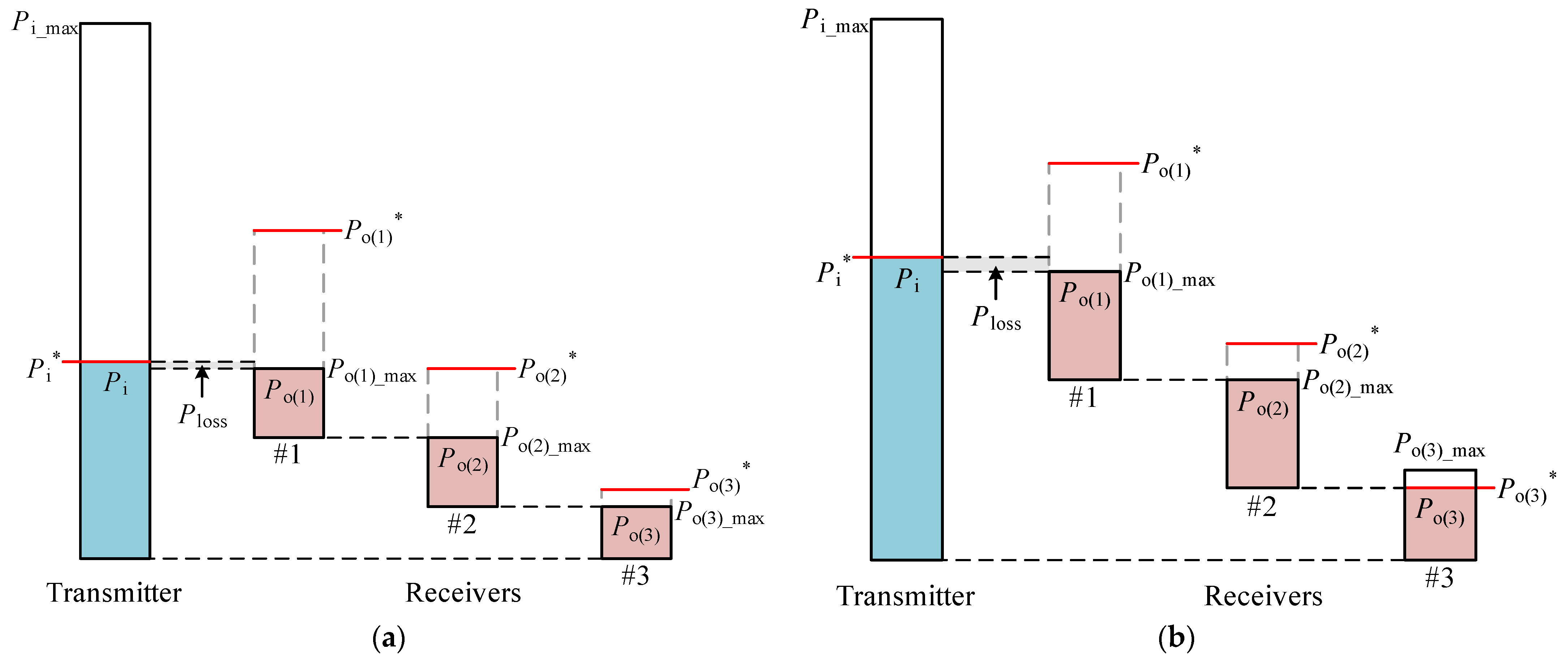
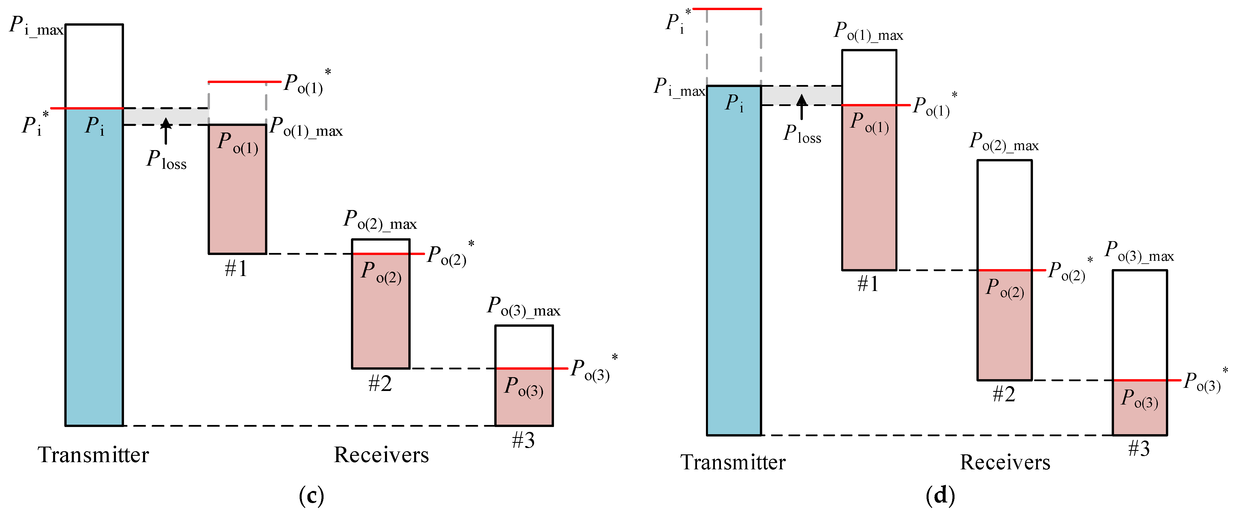
2.5. Four Typical Case Study in the Proposed Structure

Four typical stages in this example are analyzed in detail, and each specific case is represented by in Figure 10.

Case 1: P_i* is low enough, and the transmitter controller will set P_{i_norm} to a low level to ensure that P_i is equal to P_i*. Consequently, P_{o_max} of each receiver will be lower than P_o*, and all the receiver controllers will work in state 2. P_o of every receiver is equal to P_{o_max} under the control of the receiver controller. The above analysis shows that P_i = P_i* and P_o = P_{o_max}. Substituting the above relationships into (30), the slope of P_o can be derived based on (22) as:

$$\mathrm{Slope}=\frac{P_{o(i)}}{P_i^{*}}=\eta \frac{P_{o(i)}}{{\displaystyle \sum _{i=1}^3{P}_{o(i)}}}=\eta \frac{\frac{U_i^2}{L_a^2}\times \frac{{\left(M_{(i)}{D}_{(i)}\right)}^2}{R_{L(i)}}}{\frac{U_i^2}{L_a^2}\times {\displaystyle \sum _{i=1}^3\frac{{\left(M_{(i)}{D}_{(i)}\right)}^2}{R_{L(i)}}}}=\eta \frac{\frac{M_{(i)}^2}{R_{L(i)}}}{\frac{M_{(1)}^2}{R_{L(1)}}+\frac{M_{(2)}^2}{R_{L(2)}}+\frac{M_{(3)}^2}{R_{L(3)}}},i=1,2,3$$

(31)

Case 2: When the system already works in case 1 and then increases P_i* until one of the receiver controllers transfers to state 1, the system would transfer to case 2. The transmitter controller will increase P_{i_norm} to increase P_i, thereby increasing P_{o_max} of every receiver. For the receiver #3, P_{o(3)_max} will increase beyond $P_{o\left(3\right)}$*. Therefore, the controller of receiver #3 would enter state 1 and P_o(3) is equal to P_{o(3)_max}. The receiver controllers of receivers #1 and #2 remain in state 2. To sum up, in case 2, P_i = P_i*, P_o(1) = P_{o(1)_max}, P_o(2) = P_{o(2)_max}, and P_o(3) = $P_{o\left(3\right)}$*. Substituting the above relationships into (31), the slope of P_o in case 2 can be derived as:

$$\frac{P_{o(i)}}{P_i^{*}}={\eta \frac{P_{o(i)}}{{\displaystyle \sum _{i=1}^3{P}_{o(i)}}}|}_{P_{o\left(3\right)}=0}=\{\begin{array}{ll}\eta \frac{\frac{U_i^2}{L_a^2}\times \frac{{\left(M_{(i)}{D}_{(i)}\right)}^2}{R_{L(i)}}}{\frac{U_i^2}{L_a^2}\times {\displaystyle \sum _{i=1}^2\frac{{\left(M_{(i)}{D}_{(i)}\right)}^2}{R_{L(i)}}}}=\eta \frac{\frac{M_{(i)}^2}{R_{L(i)}}}{\frac{M_{(1)}^2}{R_{L(1)}}+\frac{M_{(2)}^2}{R_{L(2)}}},\hfill & fori=1,2\hfill \\ \eta \frac{0}{\frac{U_i^2}{L_a^2}\times {\displaystyle \sum _{i=1}^2\frac{{\left(M_{(i)}{D}_{(i)}\right)}^2}{R_{L(i)}}}}=0,\hfill & fori=3\hfill \end{array}$$

(32)

Case 3: When the system already works in case 2 and then further increases P_i* until another receiver controller transfers to state 1, the system would transfer to case 3. The transmitter controller will further increase P_{i_norm} to increase P_i, thereby increasing P_{o_max} of every receiver. In this example, the controller of receiver #2 will transfer to state 1. Meanwhile, the receiver controller of receiver #1 remains in state 2 and receiver controller of receiver #3 remains in state 1. To sum up, in case 3, P_i = P_i*, P_o(1) = P_{o(1)_max}, P_o(2) = P_o(2)*, and P_o(3) = P_o(3)*. Substituting the above relationships into (30), the slope of P_o in case 3 can be derived as:

$$\frac{P_{o(i)}}{P_i^{*}}={\eta \frac{P_{o(i)}}{{\displaystyle \sum _{i=1}^3{P}_{o(i)}}}|}_{P_{o\left(2\right)}=P_{o\left(3\right)}=0}=\{\begin{array}{ll}\eta \frac{\frac{U_i^2}{L_a^2}\times \frac{{\left(M_{(1)}{D}_{(1)}\right)}^2}{R_{L(1)}}}{\frac{U_i^2}{L_a^2}\times \frac{{\left(M_{(1)}{D}_{(1)}\right)}^2}{R_{L(1)}}}=\eta ,\hfill & i=1\hfill \\ \eta \frac{0}{\frac{U_i^2}{L_a^2}\times \frac{{\left(M_{(1)}{D}_{(1)}\right)}^2}{R_{L(1)}}}=0,\hfill & i=2,3\hfill \end{array}$$

(33)

Case 4: When P_i* is set high enough, the system will enter case 4. In this case, P_{i_norm} will be saturated at 1 under the control of the transmitter controller, which means that the transmitter works in state 2. Because P_{i_norm} maintains its maximum value of 1, the P_{o_ max} values of each receiver reach their maximum values and are higher than P_o*. Consequently, all the receiver controllers will work in case 1. To sum up, in this case, P_i = P_{i_max} and P_o = $P_o$*. Substituting the above relationships into (26), the slope of P_o in case 4 can be derived as:

$$\frac{P_{o(i)}}{P_i^{*}}={\frac{P_{o(i)}}{P_i^{*}}|}_{P_{o\left(1\right)}=P_{o\left(2\right)}=P_{o\left(3\right)}=0}=\frac{0}{P_i^{*}}=0,i=1,2,3$$

(34)

With the slope information of each case, the power distribution in this system in the steady state can be calculated.

This example has three receiver and four cases, and the number of cases n_case is determined by the number of receivers:

$$n_{case}=n+1$$

(35)

The total charging power is non-cooperative game, the Karush–Kuhn–Tucker could be applied to optimize the gaming relation among the receivers. The power can be inserted into the Lagrangian function as

$$L=-{\displaystyle \sum _{i=1}^n{w}_i\ln \left(p_i+1\right)}+v\left({\displaystyle \sum _{i=1}^n{p}_i-p_{total}}\right)$$

(36)

Then the partial derivatives can be derived as

$$\frac{\partial L}{\partial p_i}=-\frac{w_i}{p_i+1}+v=0,fori=1,\dots ,n$$

(37)

$$\frac{\partial L}{\partial v}={\displaystyle \sum _{i=1}^n{p}_i}-p_{total}=0$$

(38)

The KKT candidate point can be solved as

$$p_i=\frac{w_i\left(p_{total}+n\right)-{\displaystyle {\sum }_{i=1}^n{w}_i}}{{\displaystyle {\sum }_{i=1}^n{w}_i}},forv=\frac{w_i}{p_i+1}$$

(39)

$$p_i=P_i^{*},forv=0$$

(40)

Since the Lagrangian function is convex, the Hessian of the Lagrangian function is always positive definite and the derivative is the global optimal point. Then, the calculated power divisions are achieved through the duty cycle control of the DC–DC converters in the receivers. The proposed algorithm is linear, and is proportional to O(n).

For a given receiver, the combined Langrangian function can be calculated as

$$L_i=u_i+{\lambda }_i\left({\displaystyle \sum _{i=1}^n{p}_i-p_{total}}\right)$$

(41)

where λ_i is the Lagrange multiplier. Under the Karush–Kuhn–Tucker conditions, the optimization problem can be given as

$$\frac{\partial L_i}{\partial P_i}=-\frac{w_i}{p_i+1}+{\lambda }_i=0$$

(42)

Then, the charging power of each receiver is competing under the balanced condition at the power of p_total, therefore,

$$p_i=\frac{w_i\left(p_{total}+n\right)}{{\displaystyle \sum _{i=1}^n{w}_i}}-1$$

(43)

Then, the distributed power is unique. In our application, the implementation of competitive mechanism is realized by searching λ_i when the receivers need to compete on the limited total available transmitting power p_total, as shown in the flow chart in Figure 11.

The power distribution is the result of the interplay among the receivers. The total power is limited by the transmitter, and all the receivers compete for more power until their demands are met. Receivers with higher mutual inductance and low load resistance have an advantage. Finally, there will be an equilibrium. The result is that some receivers get sufficient power, while some do not. The balance itself is the result of power distribution. With the increase in the transmitter power capacity, more and more receivers can obtain the required power, and they do not compete for more power. They maintain their existing power, while others still compete for more power.

In addition, the power distribution depends on the mutual positions of elements too. So, constant, defined, and identical position between elements should be expected. Figure 12 gives the magnetic field distribution of the coils. Since the receiving coils are aligned diagonally, magnetic induction lines from one receiving coil hardly pass through the other two receiving coils. Therefore, the cross-coupling among the receiving coils can be neglected.

3. Results

An experimental multi-receiver WPT system has been built to verify the validity of the theoretical analysis.

The experimental setup is shown in Figure 13. It has one transmitter and three individual receivers. The model of all semiconductor switches in the system is Infineon IHW50N65R5, and the model of receiver rectifier diodes is CREE D3065C5.

The coil structure is shown in Figure 14. The transmitting coil has three slots designed for three receivers. Its winding consists of eight turns of Litz wire. All the receiving coils have the same structure and size. They are square-shaped with ferrite bricks over them to augment the mutual inductance. The gap between the transmitting and receiving coils is 5 cm.

The configuration of this experimental setup is listed in

Table 1. Parameters of the experimental setup.

	Symbol	Parameter	Value
	f	Frequency	85 kHz
	Ui	DC power supply voltage	110 V
Transmitter	L1	Tx coil self-inductance	91.53 μH
	C1b	Tx compensation capacitor	187.24 nF
	C1a	Tx compensation capacitor	47.97 nF
	La	Tx compensation inductor	18.85 μH
Receiver #1	L2(1)	Rx coil self-inductance	42.89 μH
	M(1)	Mutual inductance to Tx coil	16.30 μH
	C2(1)	Compensation capacitor	81.69 nF
Receiver #2	L2(2)	Rx coil self-inductance	42.20 μH
	M(2)	Mutual inductance to Tx coil	14.51 μH
	C2(2)	Compensation capacitor	85.15 nF
Receiver #3	L2(3)	Rx coil self-inductance	52.14 μH
	M(3)	Mutual inductance to Tx coil	17.61 μH
	C2(3)	Compensation capacitor	67.12 nF

. ωL_a of the LCC compensation circuit at the transmitting side is designed to be 10 ohms. The designated parameters of the compensation circuit are derived from the analysis.

The switching frequency of the receiver regulator is 50 kHz. The control algorithm is realized by programming using DSP controllers, with every transmitter and receiver having an individual DSP controller. The loads of the receivers were electric loads in the constant resistance (CR) mode. A power analyzer is connected to record the powers. In the experiment, the gate driver UCC21520 and PI controller dsp28335 have been used. The current and voltage signals are sampled and differentially amplified by AMC1302. The signal is collected through AD7682 and then transmitted back to the DSP.

The static experiment was conducted to verify the validity of the theoretical analysis, where the input power was set at the maximum value. The parameters of the controllers and the loads are shown in

Table 2. Parameters of controllers and loads.

	Symbol	Value
Load Resistance	RL(1)	12 Ω
	RL(2)	14 Ω
	RL(3)	20 Ω
Instruction output voltage	$U_{o\left(1\right)}$*	80 V
	$U_{o\left(2\right)}$*	70 V
	$U_{o\left(3\right)}$*	60 V
Equivalent instruction output power	$P_{o\left(1\right)}$*	533.3 W
	$P_{o\left(2\right)}$*	350 W
	P(3)*	120 W

. In this experiment, all the receivers were active. P_i* was swept from low to high. Each time P_i* changed, the controllers would regulate the power and, thus, the system would enter steady state again. The three receivers are terminated with 12 Ω, 14 Ω, and 20 Ω loads, respectively.

The result of the static experiment is shown in Figure 15. The optimal efficiency in the simulation is equal to 88%. With the increase in P_i*, P_i is always lower than P_i*, indicating that P_i is limited under the regulation of the transmitter controller. The total output power P_{o_sum} increases with the increase in P_i*. The difference between P_i and P_{o_sum} is the power loss of the entire system P_loss. The power distribution of this experiment is comprised of four cases: P_o curves have different slopes in different cases. With the increase in P_i*, all the receivers absorb more power until the output power P_o reaches its equivalent instructed output power P_o*. Finally, all the receivers reach their P_o* as P_i* is high enough.

The comparison shows that the experimental result is consistent with the theoretical result. However, there are some errors between the measured and theoretical values. The errors originate from the following sources: (1) Theoretical result is obtained under the assumption that the efficiency is constant; in the practical system, the efficiency increases with the increase in the power. (2) Voltage drops of the wire and semiconductor devices are not considered in the theoretical analysis. (3) The practical components of the compensation circuits and coil have tolerances. Thus, the system deviates from the resonance state. (4) The harmonic components are ignored in the theoretical analysis. Nonetheless, the theoretical analysis is in good agreement with the experimental result with acceptable errors.

A dynamic experiment is performed to verify the flexibility of the proposed method, where the input power is increased dynamically from 0 to the maximum value. In this experiment, the working condition was set to simulate a practical working condition. In a practical working condition, the system parameters may vary dynamically. For example, the coil position, load resistance, and number of receivers may dynamically change while the system is running. The proposed control method is expected to handle these variations.

This experiment simulated the condition wherein the number of receiver changes from 2 to 3. The setup is the same as the setup in the static experiment. This procedure consists of two phases. In phase 1, only receivers #1 and #3 are operated in the WPT system while receiver #2 is disabled. In phase 2, all the receivers are operated. First, the system works in phase 1 and is in steady state, then receiver #2 joins the WPT system and the system turns to phase 2. With the joining of receiver #2, the controllers regulate the power among the receivers. Finally, after the transient regulation of the controllers, the system would enter the steady state of phase 2. A power analyzer is employed to record the input and output power continuously with a period of 10 ms.

Under the theoretical power distribution condition in the steady state of phase 1, the optimal efficiency is 88%. As the condition of phase 2 is the same as that in the static experiment, the power distribution state is steady. The theoretical power distribution in both phases 1 and 2 can be determined. Figure 16 shows the power variation when the system moves from phase 1 to phase 2. At the beginning, the system is in the steady state of phase 1. The output power of receiver #2 was 0 as it is disabled, and the power only flows to receiver #3. As soon as the receiver #2 is activated at 43.2 s, the controller starts to increase the output power of receiver #2. The output power of receiver #3 decreases to the steady value in phase 2. The output power of receiver #3 decreases first, then increases, and finally maintains the same value. The regulation process lasts for approximately 3 s. Finally, the system returns to the steady state. In

Table 3. Power in the steady state in the dynamic experiment.

		Pi	Po(1)	Po(2)	Po(3)
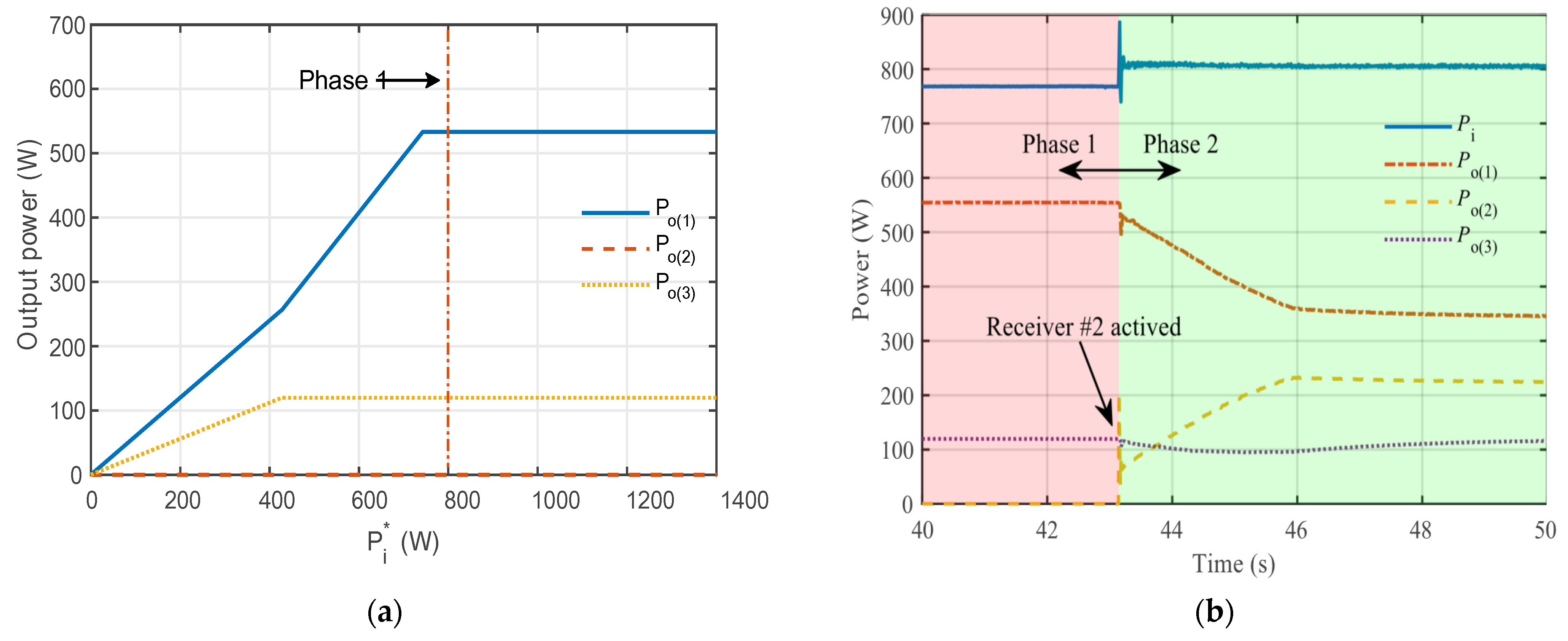
Phase 1	Theoretical	768.6 W	533.3 W	0.0 W	120.0 W
	Measured	768.5 W	554.7 W	0.0 W	119.7 W
	Error	−0.01%	4.01%	-	−0.25%
Phase 2	Theoretical	800.0 W	348.8 W	236.2 W	120.0 W
	Measured	805.7 W	343.8 W	223.2 W	119.6 W
	Error	0.71%	−1.43%	−5.50%	−0.33%

, the theoretical and measured power distributions in the steady state are compared. The measured power values match well with the theoretical power values with the maximum error of −5.50%.

The dynamic experimental result demonstrates that the proposed control method can handle the dynamic variation in the number of receivers. The power is redistributed under the combined action of all the controllers following a change in the number of receivers in the system. The control method demonstrates flexibility and robustness in the dynamic experiment. The controller works as expected even when some of the parameters vary while the system is in operation.

4. Discussion

In a practical scenario, P_i* of the transmitter controller should be the same or only slightly lower than the rated power of the DC power supply of the transmitter to prevent it from overloading. The P_i* limits the maximum power of the entire system. P_o* of the receivers should be the required power of their loads. However, the practical output power P_o may be lower than the required power due to the limit of the transmitter power capacity. The experimental setup adopts a transmitting coil designed especially for three receivers. However, the transmitting coil design is not limited. Coils with any shape, size, number of receivers, etc., are acceptable for the proposed control method. Receivers with higher power demand should be equipped with bigger receiving coil to achieve higher mutual inductance. Otherwise, the receiver may face disadvantage in the competition.

The proposed method distributes power unequally, but the competition mechanism makes dynamic distribution possible. Receivers can join or quit the system freely, and the receiver power demand can also vary dynamically. No matter how the system varies, the system will redistribute the power automatically. This control method can handle massive receivers without reprogramming, and will not become complicated with the increase in the number of receivers. Therefore, the system can expand easily.

Table 4. Comparison between existing methods.

Method	Controller Algorithm	Main Circuit Configuration	Dynamic Distribution	Scalability	Additional Requirement
Impedance matching [4,15,20]	None	Simple	No	Low	-
Multi-frequency method [19]	None	Complicated	No	Low	Multiple inverters
Time-sharing method [18]	Simple	Complicated	Yes	Low	Capacitor switching array
Frequency communication method [16]	Simple	Simple	Yes	High	High accuracy frequency measurement
Game-theory-based control [21]	Complicated	Simple	Yes	High	-
Proposed method	Simple	Simple	Yes	High	-

gives the comparison between the proposed method and some representative existing methods, and the advantages and disadvantages are listed. It demonstrates the superiority of the proposed method over previous methods. In the comparison, algorithm complexity is judged by the time and space consumed at a given input of size n [27]. The controller algorithms lower than O(nlogn), such as O(logn) and O(n), are defined as “simple” whereas those higher than O(nlogn), such as O(n^k) and O(k^n), are defined as “complicated”. Circuit configuration complexity is based on equivalent circuit topology. If the topology structure satisfies Karp–Lipton condition [28], it is defined as “simple”, otherwise it is defined as “complicated”. Dynamic distribution is judged by whether the circuit can distribute power flexibly with the change of outside factors, such as load, receiver number, or charging distance. Scalability is judged by whether this system can be applied in other multi-receiver scenarios with only changing the parameters instead of system structure. This is mainly determined by circuit topology, operating frequency and dynamic distribution.

The proposed method has a constant-voltage output characteristic. In the future, the configuration can be set to constant current output by modifying the compensation circuit and receiver controller to suit applications, such as charging batteries or supercapacitors.

5. Conclusions

A power distribution control method for a multi-receiver WPT system is proposed in this paper. By employing double-side control, the power from transmitter distributes to multiple receivers automatically. Receivers acquire power by competition, and the receivers with higher mutual inductance is easier to gain higher power. This procedure is dynamic, so the power will be redistributed when the system parameters varied. Hence, this method can handle various occasions such as the number of receivers changing, receiver power demands changing or coil position (mutual inductance) changing. For receivers, the received power will not exceed their demands, while the transmitter will not be overloaded at any given time. The control algorithm and main circuit configuration are simple, and the communication channel is not required. The increase in the number of receivers will not increase the complexity. Thus, the number of receivers can be increased easily. Static experiment with fixed system parameters indicates the power distribution result can be accurately predicted based on the circuit and controller parameters. Dynamic experiment with dynamically varying system parameters demonstrates the reliability, scalability, flexibility, and generality of this method. The proposed WPT system is compared with several others. The classification is derived based on algorithm theory and circuit topology. The characteristics are determined through mathematical calculations based on the results provided in those references.

References

- Cannon, L.; Hoburg, J.F.; Stancil, D.D.; Goldstein, S.C. Magnetic Resonant Coupling As a Potential Means for Wireless Power Transfer to Multiple Small Receivers. IEEE Trans. Power Electron. 2009, 24, 1819–1825. [Google Scholar] [CrossRef]
- Kurs, A.; Moffatt, R.; Soljačić, M. Simultaneous mid-range power transfer to multiple devices. Appl. Phys. Lett. 2010, 96, 044102. [Google Scholar] [CrossRef]
- Ahn, D.; Hong, S. Effect of Coupling between Multiple Transmitters or Multiple Receivers on Wireless Power Transfer. IEEE Trans. Ind. Electron. 2013, 60, 2602–2613. [Google Scholar] [CrossRef]
- Fu, M.; Zhang, T.; Ma, C.; Zhu, X. Efficiency and Optimal Loads Analysis for Multiple-Receiver Wireless Power Transfer Systems. IEEE Trans. Microw. Theory Tech. 2015, 63, 801–812. [Google Scholar] [CrossRef]
- Hu, X.; Wang, Y.; Jiang, Y.; Lei, W.; Dong, X. Maximum Efficiency Tracking for Dynamic Wireless Power Transfer System Using LCC Compensation Topology. In Proceedings of the 2018 IEEE Energy Conversion Congress and Exposition (ECCE 2018), Portland, OR, USA, 23–27 September 2018; pp. 1992–1996. [Google Scholar]
- Liu, W.; Chau, K.T.; Lee, C.H.T.; Jiang, C.; Han, W.; Lam, W.H. Multi-Frequency Multi-Power One-to-Many Wireless Power Transfer System. IEEE Trans. Magn. 2019, 55, 1–9. [Google Scholar] [CrossRef]
- Zhou, J.; Gao, Y.; Huang, X.; Hu, S.; Fang, Y. Voltage transfer ratio analysis for multireceiver resonant power transfer systems. IET Power Electron. 2016, 9, 2795–2802. [Google Scholar] [CrossRef]
- Kuang, J.; Luo, B.; Zhang, Y.; Hu, Y.; Wu, Y. Load-Isolation Wireless Power Transfer With K-Inverter for Multiple-Receiver Applications. IEEE Access 2018, 6, 31996–32004. [Google Scholar] [CrossRef]
- Liu, W.; Chau, K.T.; Lee, C.H.T.; Jiang, C.; Han, W. A Switched-Capacitorless Energy-Encrypted Transmitter for Roadway-Charging Electric Vehicles. IEEE Trans. Magn. 2018, 54, 1–6. [Google Scholar]
- Dai, Z.; Fang, Z.; Huang, H.; He, Y.; Wang, J. Selective Omnidirectional Magnetic Resonant Coupling Wireless Power Transfer with Multiple-Receiver System. IEEE Access 2018, 6, 19287–19294. [Google Scholar] [CrossRef]
- Huang, K.; Lau, V. Enabling Wireless Power Transfer in Cellular Networks: Architecture, Modeling and Deployment. IEEE Trans. Wirel. Commun. 2012, 13, 902–912. [Google Scholar] [CrossRef]
- Sun, T.; Xie, X.; Li, G.; Gu, Y.; Deng, Y.; Wang, Z. A Two-Hop Wireless Power Transfer System with an Efficiency-Enhanced Power Receiver for Motion-Free Capsule Endoscopy Inspection. IEEE Trans. Biomed. Eng. 2012, 59, 3247–3254. [Google Scholar] [PubMed]
- Hwang, S.-H.; Kang, C.G.; Lee, S.-M.; Lee, M.-Q. Reconfigurable Wireless Power Transfer System for Multiple Receivers. J. Electromagn. Eng. Sci. 2016, 16, 199–205. [Google Scholar] [CrossRef]
- Madawala, U.K.; Thrimawithana, D.J. A bidirectional inductive power interface for electric vehicles in V2G systems. IEEE Trans. Ind. Electron. 2011, 58, 4789–4796. [Google Scholar] [CrossRef]
- Koh, K.E.; Beh, T.C.; Imura, T.; Hori, Y. Impedance Matching and Power Division Using Impedance Inverter for Wireless Power Transfer via Magnetic Resonant Coupling. IEEE Trans. Ind. Appl. 2014, 50, 2061–2070. [Google Scholar] [CrossRef]
- Chen, L.J.; Boys, J.T.; Covic, G.A. Power Management for Multiple-Pickup IPT Systems in Materials Handling Applications. IEEE J. Emerg. Sel. Top. Power Electron. 2015, 3, 163–176. [Google Scholar] [CrossRef]
- Zhang, Z.; Tong, R.; Liang, Z.; Liu, C.; Wang, J. Analysis and control of optimal power distribution for multi-objectivewireless charging systems. Energies 2018, 11, 1726. [Google Scholar] [CrossRef]
- Kim, Y.-J.; Ha, D.; Chappell, W.J.; Irazoqui, P.P. Selective Wireless Power Transfer for Smart Power Distribution in a Miniature-Sized Multiple-Receiver System. IEEE Trans. Ind. Electron. 2016, 63, 1853–1862. [Google Scholar] [CrossRef]
- Liu, F.; Yang, Y.; Ding, Z.; Chen, X.; Kennel, R.M. A Multifrequency Superposition Methodology to Achieve High Efficiency and Targeted Power Distribution for a Multiload MCR WPT System. IEEE Trans. Actions Power Electron. 2018, 33, 9005–9016. [Google Scholar] [CrossRef]
- Lee, K.; Cho, D.-H. Analysis of Wireless Power Transfer for Adjustable Power Distribution among Multiple Receivers. IEEE Antennas Wirel. Propag. Lett. 2015, 14, 950–953. [Google Scholar] [CrossRef]
- Yin, H.; Fu, M.; Liu, M.; Song, J.; Ma, C. Autonomous Power Control in a Reconfigurable 6.78-MHz Multiple-Receiver Wireless Charging System. IEEE Trans. Ind. Electron. 2018, 65, 6177–6187. [Google Scholar] [CrossRef]
- Fu, M.; Zhang, T.; Zhu, X.; Luk, P.; Ma, C. Compensation of cross coupling in multiple-receiver wireless power transfer systems. IEEE Trans. Ind. Inform. 2016, 12, 474–482. [Google Scholar] [CrossRef]
- Zhen, N.L.; Chinga, R.A.; Tseng, R.; Lin, J. Design and test of a high-power high-efficiency loosely coupled planar wireless power transfer system. IEEE Trans. Ind. Electron. 2009, 56, 1801–1812. [Google Scholar] [CrossRef]
- Shen, D.; Du, G.; Zeng, W.; Yang, Z.; Li, J. Research on Optimization of Compensation Topology Parameters for a Wireless Power Transmission System with Wide Coupling Coefficient Fluctuation. IEEE Access 2020, 8, 59648–59658. [Google Scholar] [CrossRef]
- Roberts, M.J. Signals and Systems: Analysis Using Transform Methods & MATLAB, 3rd ed.; McGraw-Hill Education: Boston, MA, USA, 2017. [Google Scholar]
- Erickson, R.W. Fundamentals of Power Electronics; Kluwer Academic Publishers: New York, NY, USA, 2010. [Google Scholar]
- Sedgewick, R.; Wayne, K. Algorithms, 4th ed.; Addison-Wesley Professional: Boston, MA, USA, 2011. [Google Scholar]
- Fernandez, M. Models of Computation: An Introduction to Computability Theory; Springer: Berlin/Heidelberg, Germany, 2009. [Google Scholar]