1. Introduction
Heavy and high-power induction motors (IMs) are a crucial component in modern manufacturing. The complexity of the machinery used in today’s industrial machines, as well as their mechanical level, has increased with advancements in technology [
1]. Among the various elements used in IMs, bearings are pivotal because they are responsible for more than 50% of mechanical failures [
2]. Generally, electrical stress, unbalanced loads, abrasion, and overloading are the main causes of faults in rotating machinery. These faults hamper the structural integrity of IMs and create secondary faults. Failure leads to abnormalities and unpredicted downtime of the overall system, resulting in huge maintenance costs and causalities. To identify unusual signals as early as possible, it is necessary to perform condition monitoring and detect and diagnose fault information in a timely manner [
3]. In recent times, real-time monitoring has drawn huge interest in fault diagnosis processes.
Many researchers have investigated numerous aspects of condition monitoring, such as detecting and classifying various faults [
4], diagnosing the severity of faults [
5,
6], and carrying out prognoses [
7]. All these approaches require professional experience and knowledge to correctly extract fault features from signals for classification. Additionally, these processes not only require large amounts of time but are also expensive. Furthermore, high accuracy in the classification output is not guaranteed [
8]. Generally, fault diagnosis methods can be classified as reactive, preventive, or predictive maintenance methods. Among them, reactive methods are the most expensive because they take corrective measures after a fault occurs. Preventive measures require more resources for periodic monitoring, and predictive approaches depend on real-time monitoring and start taking measures after getting an indication of failure [
9]. Fault diagnosis of mechanical equipment can rely on a quantitative model, a qualitative model, or a data-driven method. The first two methods depend on the accuracy of the mathematical model and/or significant expertise related to the designed system. The last method relies on the process of data acquisition and the analysis of the measured data of the rotating machinery to classify faults [
10]. Because of improvements in communication technologies and data acquisition sensors, data-driven methods of fault diagnosis have become a preferred choice for researchers. Data acquisition, data preprocessing, feature extraction-selection, and fault classification with a preferable algorithm are the main steps of data-driven fault diagnosis techniques.
The diagnosis of induction motor faults is performed mostly by using different signals acquired from motors, such as vibration signals [
11], acoustic emission signals [
12], motor currents [
13], temperature, and thermal images [
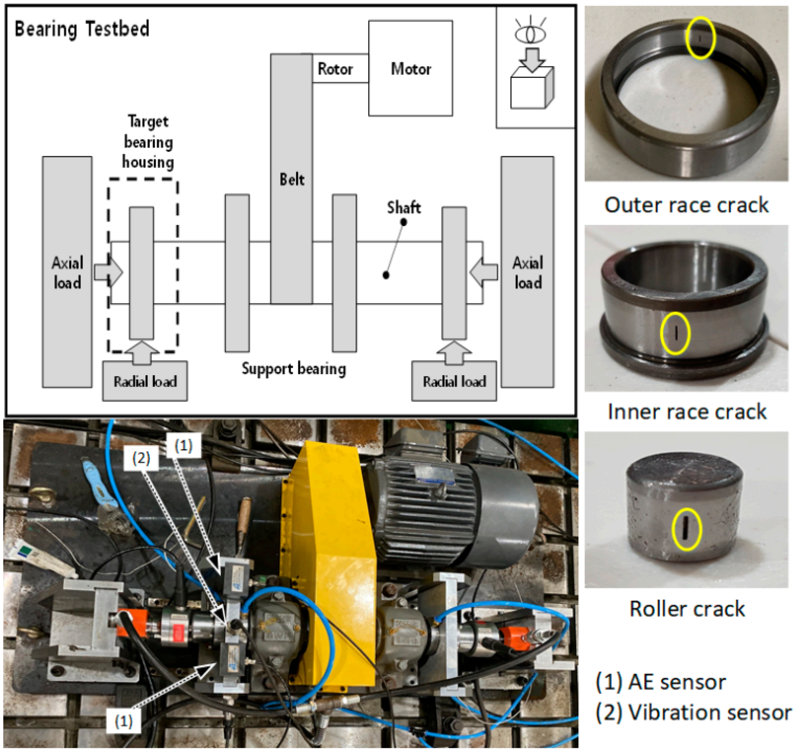
14]. In vibration signal-based methods, the signal is acquired through vibration sensors. Then, the frequency analysis is performed for further fault investigation. In this case, sensors are installed around the bearings under investigation, and full-time access is mandatory for recording and acquiring data. Despite containing a huge number of data related to a mechanical fault in vibration data, accurate extraction of fault characteristic signals is extremely important due to the noisy environment around the examined components [
15].
Signal processing techniques play an essential role in preprocessing as well as in feature extraction. Most signal processing techniques consist of time-domain analysis, frequency-domain analysis, or time-frequency domain analysis [
16,
17]. Generally, the peak-to-peak amplitude, kurtosis, root mean square, and higher-order statistical moments are calculated and used as features in the time-domain approach. Fast Fourier Transform (FFT) and spectral analysis are the most popular approaches for frequency-domain analysis. Finally, due to the nonstationary nature of the vibration signal, analysis based on the time-frequency domain is more suitable for bearing fault analysis; this includes techniques that use the wavelet transform [
17], short-time Fourier transformation (STFT) [
18], singular value decomposition [
19], local characteristic-scale decomposition (LCD) [
20], local mean decomposition (LMD) [
21], empirical mode decomposition (EMD), or ensemble empirical mode decomposition (EEMD) [
22]. Because it is controlled with the basis function, the wavelet transform cannot attain adaptive decomposition in many cases, which is a major drawback for signal analysis. Additionally, choosing an accurate mother wavelet for certain types of fault signals is a challenging task. EMD is widely used to deal with nonlinear and nonstationary signals, although it possesses large data dimensions and low calculation efficiency because it includes redundant information [
23]. Additionally, mode mixing is a problem for EMD, where the same IMF can contain oscillations with different time scales. Additionally, signals containing the same time scales are assigned to different IMFs. As a result, the IMFs do not accurately reflect the real scenario, and the actual properties of the signal can be misinterpreted. In this analysis, the EEMD method is applied to a vibration signal to solve the mode mixing problem of EMD when separating the decomposed signals to IMFs.
Envelope detection (ED) is another effective method used in fault diagnosis. This high-frequency resonance technique was introduced by Mechanical Technology Inc. [
24,
25]. A narrow-band, envelope spectrum-based algorithm was applied by Klausen et al. [
26], which can autonomously detect bearing faults by investigating multiple narrow bands of various faults. In [
27], the authors presented an effective technique, named envelope demodulation, to accurately find the fault signatures in a bearing. Additionally, Tyagi et al. [
28] proposed a method based on the optimum envelope window to overcome shortcomings of the traditional envelope detection process by using a particle swarm optimization technique for bearing fault analysis. Different envelope detection techniques with spectral correlation and RMS-based methods can identify different bearing faults. Different techniques can also increase the computational speed [
29]. In [
30], EMD is employed to find an accurate resonant frequency, with the help of envelope analysis for verifying the characteristic fault frequencies; this can be used to efficiently identify the bearing faults. The efficiency of the envelope analysis method largely depends on choosing suitable filter parameters. For this purpose, the fast kurtogram method has been analyzed by many researchers [
31,
32,
33]. Envelope analysis based on the kurtogram method is an effective and convenient approach that can be used to diagnose bearing faults.
Machine learning (ML) algorithms are widely used for fault diagnosis, as fault data are available from many devices of interest. In [
34], the empirical wavelet transform, fuzzy entropy, and support vector machine (SVM) are applied for signal decomposition, computing model inputs, classification, and predicting faulty conditions. In [
35], a model for fault classification is built with extreme machine learning, which can extract multi-scale features from the original signal. Among other approaches, K-nearest neighbors (KNN) [
36], random forest (RF) [
37], and artificial neural networks (ANN) [
38] have been successfully implemented for fault diagnosis. Although ML-based fault diagnosis techniques are performed well and are well-organized, they also have some drawbacks. First, to make the ML model highly accurate, it needs to extract discriminative features with signal processing techniques, which require expertise and lots of time. Second, a similar feature extraction and selection process for a particular type of signal might not provide satisfactory results for other signals.
In recent times, deep learning (DL) algorithms have been used in various technical and research fields. Among them, robot vision [
39], control systems [
40], and power capacity allocation [
41] are some of the most advanced examples. Deep learning has also become a promising technique in fault diagnosis because of its capability of automatic feature learning from the original signal. It possesses nonlinear operations for multiple stages and performs classification based on automatically extracted high-level features. DL consists of three parts: a deep auto-encoder (DAE), a convolutional neural network (CNN), and a deep belief network (DBN) [
42]. Among recent studies, combining time and frequency domain features with a sparse auto-encoder and DBN is a popular approach for bearing fault investigation. Several DBN-based fault diagnosis approaches are published in [
43,
44,
45]. The CNN method makes the training process easier because it shares weights and has sparse connection ability. It has also attracted the attention of researchers for use in more complex scenarios. Variations of CNN have been applied to the raw signals from various noisy environments for the diagnosis of bearing faults. More details can be found in [
46,
47,
48].
Generally, a representation of a 2-D image explores the local texture fault features, which can be obtained by applying a time-frequency-based transformation from the time-domain signal. This method has proven to be efficient for fault diagnosis with a vibration signal [
49,
50]. In this case, a 2-D image constructed from only time-domain signals may not contain the fault characteristics effectively. To address this issue, in this paper we propose an approach that utilizes EEMD to select dominant modes and then transforms the vibration signal into 2-D images for accurate bearing fault classification. In recent times, 2-D images from vibration signals have been generated using an energy distribution map [
51] and bi-spectrum analysis [
52], in which discrimination among individual bearing faults are projected. However, these techniques are unable to show the relationship between the fault signatures and the projected image. Significant information related to bearing health can be collected from the periodic impulse behavior due to the rotation at a constant speed and precise transient response analysis, which can provide fault indication at an early state. The periodic transient response generates peaks at different frequencies, such as the inner race fault frequency (FI), outer race fault frequency (FO), and ball spin harmonics (SF). Additionally, the performance of the fault diagnosis can be improved by observing signals from these particular frequency ranges [
36,
53].
In the majority of works, after EEMD decomposition, statistical, time domain, and frequency domain features are created and used for fault classification with machine learning algorithms. In this work, the innate ability of CNN with image data is leveraged by using 2-D images in the training phase. Our proposed approach utilizes selective intrinsic mode functions (IMFs) from EEMD and wavelet transform to generate an image dataset. Of all the IMFs produced after performing EEMD on vibration signals, the most relevant IMFs are selected based on kurtosis value. Thus, the selected IMFs contain the fault signature, which is validated by performing envelope analysis. Envelope analysis ensures that even after reconstruction the signal still contains the fault components. After selecting the one-dimensional IMF components, they are converted into two-dimensional spectrogram images using continuous wavelet transform (CWT), which is a technique of transforming the time-domain signal into a time-frequency domain based on Fourier Transform (FT) and Short-Term Fourier Transform (STFT). Comparing to FT and STFT, the application of wavelet transform is favorable because it can extract temporal and spectral information. The basic idea of wavelet transform is to find the correlation of a mother wavelet (a zero-averaged waveform of effectively limited duration) with a signal of interest at different points. The shape and position of the mother wavelet can be varied using its scale and location parameter. There are several mother wavelets available for finding a distinctive shape within a signal. Generally, the similarity of the mother wavelet basis function and the inspected signal plays the main role when choosing the most appropriate wavelet.
In addition, images generated from raw vibration signals with two other techniques, conventional wavelet spectrogram, and defect signature wavelet image generation method [
54] are also used to train the CNN model to establish the validity of our proposed image generation technique. Finally, a CNN is trained with a portion of this image data. Two well-known CNN architectures, namely, AlexNet and LeNet, are also trained with the same data to compare our proposed model.
The major contributions of this work can be listed as follows:
A pipeline to convert 1-D (the IMFs obtained from vibration signal after EEMD) signal to 2-D image signal involving CWT.
A CNN-based classifier model for bearing fault classification. The CNN architecture is less complex as a small number of hidden layers is used.
A laboratory dataset collected from a bearing testbed with multiple bearing faults is used to validate the performance of the described approach. Additionally, some other well-known CNN methods described in the literature are applied for comparison.
The rest of this paper is organized as follows.
Section 2 presents the test rig, description of the experiment setup, and details of the data acquisition process.
Section 3 provides a detailed description of the overall process utilized in this paper to investigate various faults.
Section 4 explains the experimental evaluation of the proposed approach from the dataset using the evaluation parameters. Our proposed method is also compared with state-of-the-art approaches. Finally,
Section 5 includes our concluding remarks.
3. Proposed Bearing Fault Classification Approach
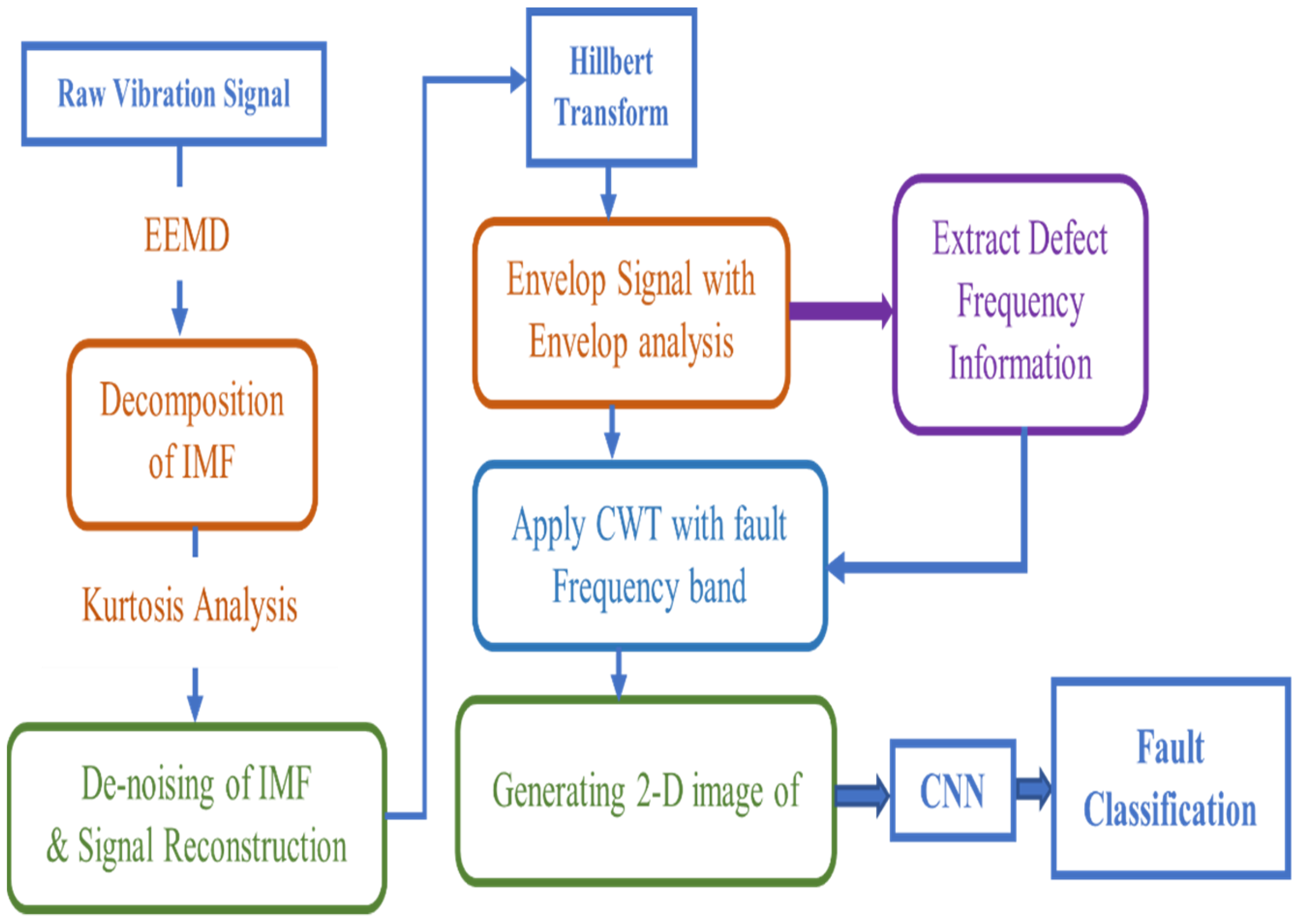
The main target of this study is to classify different bearing faults by investigating the vibration signal using a convolutional neural network. CNNs are well suited for classification from 2-D images, but the vibration signal is 1-D in nature. Therefore, in this paper, an approach is proposed that can transform the vibration signal into a 2-D image to take advantage of the CNN model. By applying EEMD, the intrinsic mode functions (IMFs) are calculated; these represent the decomposition of the vibration signal in different frequency bands. However, it has been observed that not all of the decomposed IMFs contain useful information pertaining to the faults. To find the dominant IMFs, the kurtosis value is utilized. Additionally, reducing the number of IMFs will reduce the computation complexity. Finally, the selected IMFs that contain fault information are used to rebuild the signal. After that, the new signal is transformed into a 2-D image using CWT with the particular fault frequency range. The proposed method is presented in
Figure 2 and explained in the following sub-sections.
3.1. Ensemble Empirical Mode Decomposition (EEMD)
To deal with nonlinear and nonstationary signals, Haung et al. [
55] proposed a signal analysis method in 1998 referred to as empirical mode decomposition (EMD). This approach decomposes any complex signal into a residual portion and several multi-scale intrinsic mode functions (IMFs). Every IMF is represented by a function, which must satisfy two conditions:
The extrema points and the number of zero crossings must be less than or equal to 1 for the overall dataset.
The mean value of the local maximum envelope signal and the envelope defined by the local minima are zero at all points.
Although the resultant signal obtained after performing EMD includes most of the vital information of the raw time signal, it experiences an endpoint effect and mode mixing problem where a portion of the IMF may have properties that are quite similar to adjacent IMFs. To solve this issue, Wu and Huang [
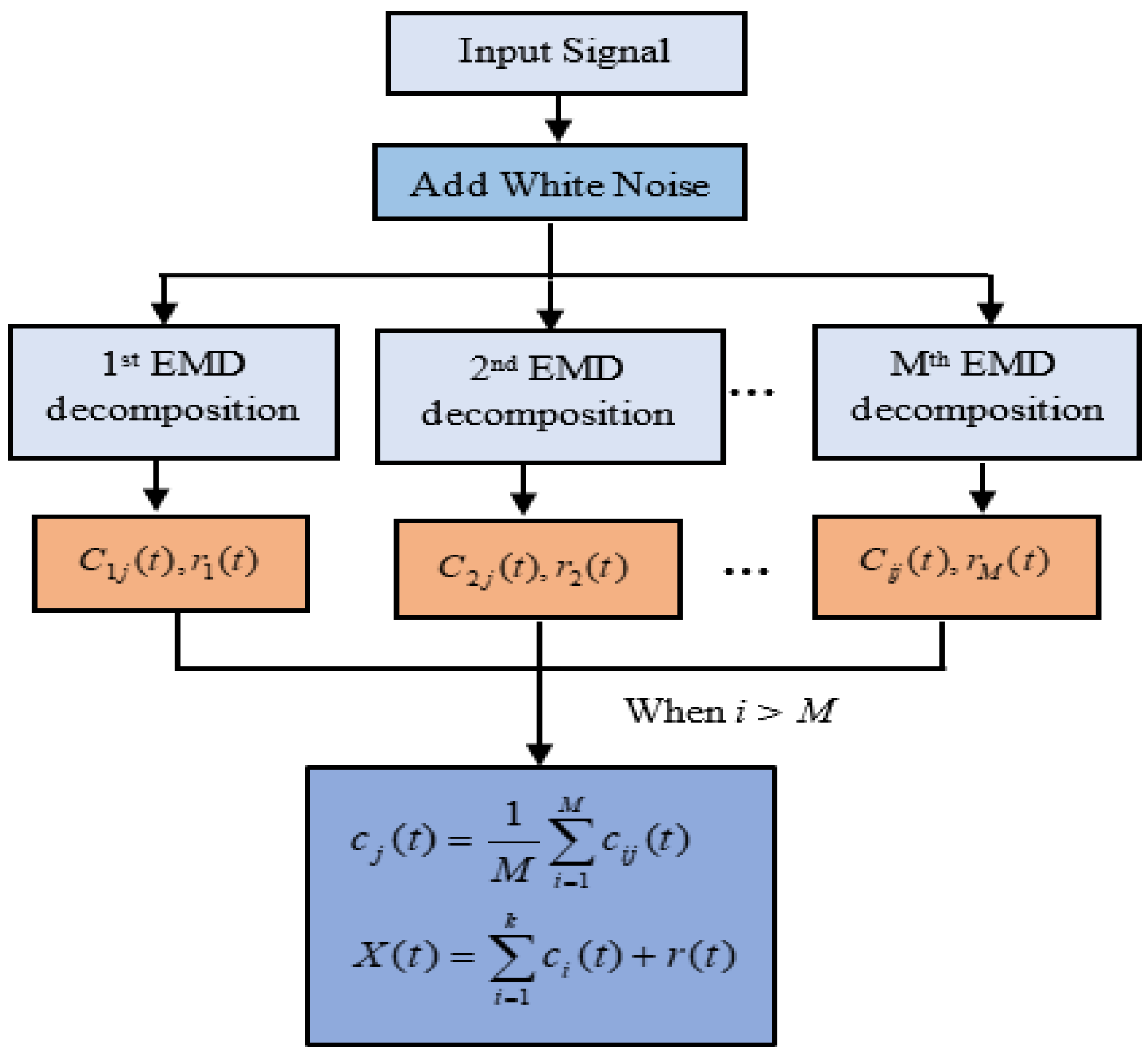
56] proposed the ensemble empirical mode decomposition (EEMD) method, in which white noise was first added to the signal and then EMD was implemented to reconstruct a new signal. The resultant signal comprises the average values of all modes and efficiently eliminates the limitations of EMD to generate a more accurate set of true IMFs. The basic steps of the EEMD method are given below:
Step 1: White noise is added to the original time series data.
where
i = 1, …,
M and
represents the white noise, which has a new normal distribution for each trial. Additionally,
M indicates the number of trials.
Step 2: The updated time-series signal is decomposed by EMD and all the IMFs
and one residual component
are extracted.
Step 3: If i < M, repeat step 1 and step 2 by adding different series of white noise every time to get the ensemble of IMFs.
Step 4: All the ensemble IMFs are calculated by taking the average as follows:
Here, represents the j-th IMF value decomposed by EEMD (j = 1, …, N) when the i-th white noise is being added.
The workflow of the EEMD method is presented in
Figure 3.
The eight IMFs and one residual signal for the roller bearing are presented in
Figure 4, where each IMF contains an individual frequency range. The corresponding Fourier spectra for each of the IMFs are shown in
Figure 5, clearly exhibiting that, with EEMD, the generated IMFs contain the signals of different frequency ranges.
Though the EEMD method solved the mode mixing problem, it is still necessary to find out the most important IMFs that exhibit substantial fault information. The resultant IMFs possess high cardinality and can be signal- or noise-dominant functions. Therefore, using all IMFs in fault detection may result in lower efficiency, as not all IMFs contain fault information. If the number of selected IMFs becomes too low in the selection state, useful information related to faults may be skipped and the accuracy of fault detection could be low. On the other hand, too many IMF components can create confusion between effective feature information and false components, as well as increase the computational complexity [
57]. Several methods are proposed for designing an efficient fault diagnosis system by identifying appropriate IMFs for a faulty condition. For example, Lei and Zuo [
58] utilized a sensitivity factor calculated from a correlation coefficient to select IMFs. In [
59], a degree-of-presence and Kullback-Leibler divergence-based matrix was introduced for selecting informative IMFs.
Kurtosis values of IMFs can also be used to select the most suitable IMFs related to fault signatures, as demonstrated in a few previous studies. This statistical indicator is utilized in [
31] to detect the impulse components that occurred due to the presence of faults in signals. In [
60], based on the kurtosis value, an IMF selection method is used with the EEMD method to extract fault signatures. After that, with the reconstructed signal, the characteristic frequency ratio was calculated between healthy and faulty bearings, and a lower boundary was applied to distinguish between them.
Kurtosis is a higher-order statistical feature of time series data. The kurtosis value of a time series observation indicates how outlier-prone the time series distribution is. Kurtosis of a time series observation is expressed as:
Here,
xi is the
i-th time series point, while
μ,
σ, and
N represent the mean, standard deviation, and length of the time series data, respectively. Changes in the kurtosis value of time series data point to corresponding changes in the physical system from which the time series data was obtained. Generally, when a normal distribution is considered, the value of kurtosis is equal to 3. In
Figure 6, kurtosis values of random observations from the dataset in use are presented. It can be noticed that when the bearing is not faulty the kurtosis value is very close to 3. Alternatively, for a bearing with a fault, the kurtosis of the time series data is much higher than 3. Therefore, in this work, the value of kurtosis is considered a crucial parameter that can be used to discover relevant IMFs, in which fault information is significantly noticeable.
The original signals and reconstructed signals after removing the unnecessary IMFs based on kurtosis for every bearing condition are presented in
Figure 7.
3.2. Envelope Analysis for Bearing Fault Analysis
When operating rotating machinery, various types of damage, such as pitting, misaligned raced damage, spalling, and waviness can occur because of manufacturing malfunctions, incorrect installation, material fatigue, and so on. Each type of bearing fault can be characterized by a specific frequency, which depends on various parameters associated with the geometric characteristics of the bearing. The fault-specific frequency occurs due to the increase of the vibration energy because of the interaction between the defects and the bearing surface. The defect frequencies for the inner race fault (FI), outer race fault (FO), and roller faults (SF) can be defined as:
Here, , , , and define the ball numbers, the ball diameter, the diameter of the cage, the contact angles of the balls, and the rotational frequency, respectively.
A high peak is generated in the FFT spectrum because of the increasing energy. Generally, in the high-frequency region, it becomes difficult to distinguish the damage frequency with the FFT method because of the amplitude modulation. To resolve this matter, the Hilbert transform is combined with envelope analysis, which is used as a demodulation technique. This helps to amplify the fault impulse with a bandpass filter, which includes the fault frequency range and rejects the carrier signal.
However, when the FFT is applied to generate the envelope spectrum, it may lose some time information regarding the exact time in which the impulse appeared. To address this issue, a new spectrogram produced by the continuous wavelet transform (CWT) is utilized; this represents the time and frequency domain signal envelope [
54].
The main idea of the Hilbert transform is to transfer the time domain vibration signal into the Hilbert domain,
, by applying the convolution between
s(
t) and the signal
, which implies [
] [
61]. The convolution results in a signal with a complex form, which can be defined as
. Then, the signal envelope is computed as the absolute value of
with
. The envelope spectrum is presented in
Figure 8 and is then obtained with the square root of the FFT and the envelope signal. Considering the mathematical approach, the rectified signal is equivalent to the square root of the squared signal, which is also true when calculating the envelope signal. It is better to apply the square root operation, which helps to visualize superfluous components of the original signal, which can make it difficult to extract useful information. Additionally, it is not easy to remove high harmonics with a low pass filter or create aliasing in the required measurement range. The convolution method produces results with various frequencies, including the spacing of sidebands, which contains the modulated information of the desired signal. Next, the resultant envelope signal is used as an input for the continuous wavelet transform.
3.3. Generating a 2-D Defect Signature Image with a Wavelet Transform
The CWT is recognized as an appropriate method for investigating nonlinear and nonstationary signals since it shifts a time-domain signal into a time-frequency domain. As the result, this method yields correlation coefficients through a convolution operation between a mother wavelet and the original signal. There are two important parameters associated with mother wavelet functions. The first one is a scaling parameter, which allows for modifying the shape of the mother wavelet by stretching or contracting. The second parameter is called the shifting parameter and helps to control the movement of the mother wavelet function along the signal being investigated. By varying the scaling parameter and performing shifting with the mother wavelet, the dynamic frequency characteristic of the signal can be obtained.
The process of detecting the rolling-element bearing local faults using the wavelet transform has been analyzed by many researchers. Here, the filter includes the fault-associated frequency band to create a 2-D representation after generating the envelope signal. The squared module values of the wavelet coefficients and analyzing the squared envelope signals in the frequency domain help extract important information for fault diagnosis. Each type of fault is associated with the specific fault frequencies, and the envelope analysis can be used to extract repetitive transient peaks in the frequency domain as well as the modulation patterns depending on the fault types.
When the time-frequency analysis is more important than the localization of transient points for an oscillatory signal, the bump wavelet is considered a better choice than the mother wavelet. It provides better separation of start and end times for every component and can be used to achieve high precision in every completed test. The relationship of the scale and center frequency of this symmetrical frequency wavelet can be expressed as follows:
Here,
σ >
0, v >
0, and
σ, v >
1, which is the general convention for CWT. In this equation, the window lengths of the wavelets can be controlled by adjusting σ, and this can also modify the shape of the transformed signal. The bump wavelet provides good frequency localization in comparison with other existing wavelets due to its band-limited characteristic. In Equation (5),
represents the indicator function and the peak frequency is denoted by
, where
. However, the different fault signature characteristics associated with the mother wavelet location and properties of the subsequent child wavelet are controlled by the translation matrix,
v. Regarding the vibration signal, the slow variation elements are captured by the stretched wavelet, whereas the fast variation elements are captured by shrinking the wavelet. Due to this property of the wavelet transform, the signals containing different types of frequency components can be efficiently investigated. Also, it provides the foundations for analyzing any concealed elements of the transient impulse. The bump wavelet possesses a symmetrical representation concerning the peak frequency. It worth noting that since the mother wavelet acts as a band-pass filter, the defect frequency ranges should be specified. To determine the fault frequency ranges accurately and extract the fault information precisely, it is necessary to analyze the fine-resolution frequency band. During this analysis, multiple fault frequencies of bearings are analyzed by varying the cutoff frequencies of the bandpass filter. The range of wavelet coefficients can be defined as below:
Here,
and
k represent the highest defect frequency of the sideband and the allowed number of the harmonic, respectively. However, the range of the cutoff frequency starts at 0 Hz for determining the fine resolution in terms of the frequency. These provisions are used to create 2-D coordinate matrices. Using the colormap, the vertex colors are defined such that they correspond to the coefficients of the matrix, which finally results in a 2-D spectrogram, provided in
Figure 9.
Finally, the generated 2-D images are divided into training and testing datasets and are fed into the input of the CNN model.
3.4. CNN Model
The convolutional neural network (CNN) is one of the most effective models in deep learning. It was mainly introduced to deal with images. The CNN model can automatically learn high-dimensional features, which makes it very effective in target detection, optical character recognition (OCR), video analysis, and image classification applications. Overfitting is a common problem in machine learning methods, but this can be solved with CNN by performing large-scale deep learning and sharing weights [
62]. The CNN model is predominately made up of a convolution layer, pooling layer, fully connected layer, and output layer. Due to its complex mechanism, it can easily reveal the inner rules and diverse presentation levels of sample data. It can also reduce the dependence on training data with the help of some optimization parameters, such as batch normalization, dropout layers, rectified linear units, and so on [
63].
3.4.1. Convolution Layer
The core building block of the CNN model is known as the convolution layer. This is the segment of the network where heavy computation occurs. The convolution layer consists of several learnable kernels, and convolution operation is carried out between these kernels and the input image to produce feature maps. Then, it provides inputs to the activation functions to perform a nonlinear operation. After completing the overall process, a 2-D image will be mapped into a different feature matrix. The convolution operation can be defined as:
Here, is the output of the convolution layer, i and j mean the i-th input feature map and j-th output feature map, respectively. Additionally, l represents the l layer, implies the i-th input feature map in the (l − 1) layer, is the weight matrix, contains the bias value, and f(.) indicates the activation function. Among various activation functions, ReLU is most used because of its ability to increase nonlinearity in CNN, which can be represented as . When the input data has high variations with large complexity, several convolution layers are used to build a deep CNN to diagnosis all variant features accurately.
3.4.2. Pooling Layer
The pooling layer is a down-sampling layer generally linked with the convolution layer to reduce the size of the feature map to reduce the network computation time and maintain the same invariance of the distinctive characteristic scale. This reduction is performed by keeping the exact features unchanged and making the output less sensitive to environmental change. Among different pooling approaches, such as average pooling, max pooling, logarithmic pooling, and norm pooling, max pooling is largely applied in CNN. This can be written as follows:
Here, and denote the (a, b) pixel of the ith feature map after and before the max-pooling operation, respectively. Further, p expresses the stride size of the pooling window, which should be greater than 1. However, if p becomes too high, information related to that CNN layer may be lost.
3.4.3. Fully Connected Layer
The fully connected layer takes the results from the convolution and pooling layers and classifies the image. In this work, the SoftMax activation is used in the dense layer to classify different classes. The output of the fully connected layer can be defined as:
Here, , , , and represent the output of the fully connected layer, feature vectors (one-dimensional), weight coefficients, and bias, respectively.
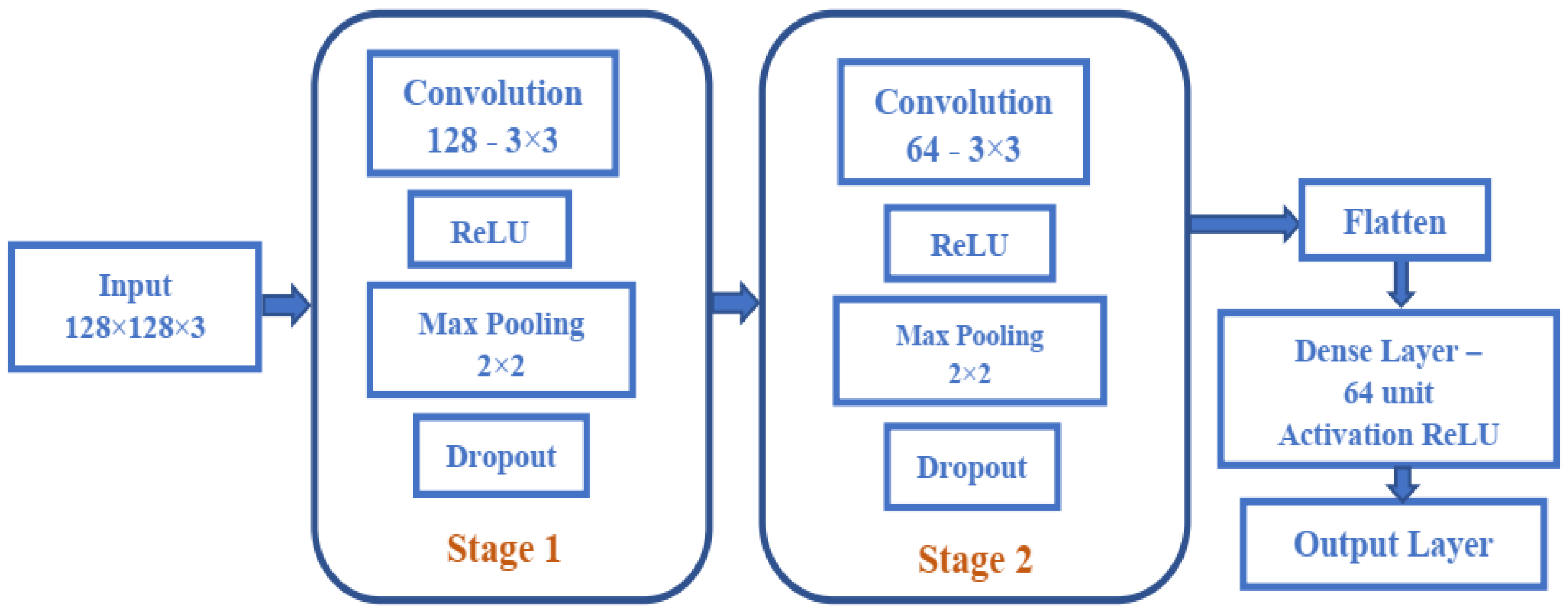
The CNN model implemented in this work includes two convolution layers with 32–3 × 3 and 64–3 × 3 filters for an input image size of 128 × 128 × 3. Here, 128 represents the image length and width and 3 indicates the three channels of the RGB image. The max-pooling layer has a size of 2 × 2. Additionally, to ensure better regularization in each layer, a dropout value of 0.5 is applied. The structure of the CNN model used in this study is provided in
Figure 10.
In this CNN model, the trainable parameters are first initialized and then optimization is performed with the adaptive moment estimation (Adam) algorithm to reduce the error between the original and predicted values. The categorical cross-entropy is applied to measure the training error. Several types of CNN models were examined by varying each of the described layers, and it was observed that the extensive deep version of CNN not only failed to provide better accuracy but also took a large amount of time for training. The proposed CNN model runs at 50 epochs to extract features for each type of bearing condition. Other conventional deep neural network architectures, such as LeNet-5 [
64] and AlexNet [
65], were also trained with the same 2-D image to allow for comparison with the results of the proposed model.
3.5. Performance Evaluating Parameters
The performance of the proposed model was initially described with a confusion matrix, which gave a numerical representation of correct and incorrect predictions made by the model. Later, some other evaluation parameters, such as the precision, sensitivity, specificity, F1-score, and overall accuracy, were computed from the entries of the confusion matrix.
Table 2 lists the expressions for the parameters. Here, TP, TN, FP, and FN correspond to true positive, true negative, false positive, and false negative, respectively.
4. Experimental Results
The vibration signal recorded from the testbed described in
Section 2 is converted into a 2-D image. Each observation of the vibration signal has a duration of 1 s. To produce a distinctive image dataset for the CNN model, each instance of the signal is passed through EEMD decomposition, signal reconstruction, envelope analysis, and spectrogram creation.
Figure 9. depicts three sample spectrogram images for different fault conditions, which are distinguishable by visible inspection. Later, the proposed CNN model is employed with the images containing the invariant signatures of different faults to automatically extract and learn features. While training the CNN model, a total of 988 samples is considered for training purposes. After that, 248 samples are used simultaneously for validation during every epoch. To validate the proposed method, two other popular CNN models, i.e., AlexNet and LeNet-5, are trained with the same dataset. The classification results for these models are compared with the proposed model. Additionally, two other methods, i.e., the conventional wavelet spectrogram (CWS) and the defect signature wavelet image (DSWI) generation method [
54], are applied to create 2-D images. These images are compared with the image created using the proposed method.
Figure 11. displays the images for different conditions produced by the three approaches.
Here, the images generated from the conventional wavelet spectrogram do not reveal any distinct fault signatures for any fault conditions of the bearings. However, the other two methods do show different patterns depending on the fault that occurs in the bearings. More specifically, because we applied EEMD on the original signal and reconstructed the signal based on the kurtosis value, our proposed method generated images that show more noticeable differences between the different fault signatures. This method also indicates a strong correlation with the specific damage frequencies. This type of image can be provided as the input to the CNN model to evaluate the classification accuracy. The confusion matrices obtained from the proposed model for three different image generation techniques from the vibration signal are provided in
Figure 12. From the confusion matrices, it can be observed that the image generated with the proposed method, i.e., a combination of EEMD and envelope analysis with CWT, shows comparable classification performance.
Two CNN architectures commonly used for image processing, i.e., AlexNet and LeNet-5, are also trained with the generated images. The confusion matrices obtained for all of these CNN models are given in
Figure 13. The accuracy values indicate that every model is very successful in classifying the faults. Thus, it indicates that the image dataset produced from our proposed approach is quite efficient for bearing fault diagnosis.
Other evaluation parameters are presented in
Table 3 for comparison. AlexNet and LeNet exhibit slightly better performance when images produced with our proposed method are used. Additionally, when the CNN architecture discussed in this paper is combined with the image set, an accuracy of 99.19% is achieved, which is slightly higher than the other two models.
The DL models were running on Windows 10 having a 3.60 GHz CPU of Intel with 16 GB RAM. With the constructed 2-D images corresponding to different bearing faults, the LeNet, AlexNet, and our proposed CNN model took 303.177 s, 983.20 s, and 503.568 s, respectively, to produce the outputs. The training time can be reduced significantly by using GPU programming-based implementation. Observing this, it can be concluded that the LeNet model is faster than the other two, but the proposed model attains the highest accuracy although its training takes twice more time than the LeNet model.


