1. Introduction
Colorectal cancer is the third most common type of cancer with ≈1.9 million new cases and ≈935 thousand deaths yearly [
1]. At the time of diagnosis, approximately a quarter of the patients already have cancer spread into the liver in the form of metastasis [
2,
3]. Detection, definition and mapping of these metastases require medical imaging.
Medical image segmentation is the process of locating and extracting the anatomical structures of interest or pathologies from medical images such as computed tomography, magnetic resonance imaging, ultrasound, etc. Extraction of hepatic vessels and their relationship with tumors play an important role in liver surgery treatment and planning [
4]. In addition, liver vessel extraction aids in visualization, liver segment approximation, multi-modal registration, where vessels act as landmarks, computer-aided diagnosis and surgery [
4,
5]. The manual delineation of hepatic vessels is often time-consuming, error-prone and highly user dependent. Image-related challenges, such as high signal-to-noise ratio, low image resolution, inhomogeneous background, varying contrast between the vessels and liver parenchyma, imaging artifacts and varying vessel thickness [
6] make hepatic vessel segmentation challenging. In recent years, deep learning-based methods have become widely used for various medical image analysis tasks. Though deep learning-based segmentation is proven to be efficient, the way of data handling and the enhancement of images that go into the deep learning model has a major influence on the precise segmentation. Especially for complex structures such as vessels, enhancement techniques are proven to be effective prior to segmentation and visualization [
7,
8,
9]. In particular, Hessian-based vessel enhancement filters are most popularly used compared to other techniques [
10,
11,
12,
13,
14].
In this work, the impact of four different multi-scale vesselness filters, including Hessian, Sato, Frangi and Meijering, were studied experimentally. The effect of enhancement has been evaluated based on 3D U-net, a widely used deep-learning based segmentation model in the medical imaging domain. To review the impact of enhancement on segmentation, we compared the segmentation results with and without vesselness enhancement. We also compared the performance of different multi-scale vesselness filter. Secondly, we studied the effect of gamma filtering on vesselness enhanced images. Finally, we proposed to fuse the outcome from the filtered and gamma corrected images in two different designs, and the effect of fusing the outcome is compared over the individual vesselness filter. We evaluated the methods on the clinical dataset.
2. Related Work
In Frangi et al. [
10], the vesselness measure is obtained based on all eigenvalues of the Hessian, a multi-scale second order local structure of the image. Yang et al. [
12] improved the multi-scale enhancement technique inspired by Frangi et al. [
10] to enhance the vessel structures for retinal vessel segmentation. Kumar et al. [
15] developed a modified multi-vesselness filter based on the Hessian matrix for the center line extraction of blood vessels. In Drechsler et al. [
13], the enhancement method is based on the Laplacian for the tubular structures. Jerman et al. [
14] implemented a enhancement filter based on the ratio of multi-scale Hessian eigenvalues to accurately enhance the borders between the vessel structures and the background. In Lamy et al. [
16], seven different Hessian based vesselness filters were compared and benchmarked on the IRCAD and VasucSynth datasets. The enhancement methods were evaluated using level-set-based segmentation. Zeng et al. [
17] proposed a Hessian-based multi-feature method to segment the liver vessel structures prior to segmentation based on the extreme learning machine. Manh Luu et al. [
18] evaluated five different diffusion filters for enhancing the liver vessels in 3D CTA images. In Phellan and Forkert [
19], different vessel enhancement algorithms were applied to time-of-flight MRA images for cerebrovascular segmentation and then compared.
In Shahid and Taj [
7], a combination of adaptive histogram equalization, morphological top-hat filter, high boost filtering and Frangi filter were employed for the purpose of retinal vessel enhancement prior to deep learning-based segmentation. In Soomro et al. [
8], morphological operators and the contrast limited adaptive histogram equalization (CLAHE) technique were used to enhance and segment the retinal vessels. In Blaiech et al. [
9], to study the effect of enhancement, CLAHE, Frangi and ranking the orientation response of path operators(RORPO) were used to enhance the coronary artery for the purpose of segmentation.
Gamma correction is widely used in the medical image enhancement process. In Karuppanagounder and Palanisamy [
20], a gamma correction-based technique is used to enhance medical MRI and CT images. In Tiwari and Gupta [
21], a combination of gamma correction and homomorphic filtering was used to enhance knee MRI images. In Dash and Senapati [
22] and Zhitao et al. [
23], the combination of gamma correction with other enhancement techniques was used to enhance the retinal blood vessels from the ophthalmic images.
In the field of medical image segmentation, 3D U-net [
24] based architectures are widely used for various volumetric segmentation tasks [
25].
Inspired from the literary works, in this paper, we also studied the effect of the combination of Hessian-based vesselness filters and gamma-correction technique for the hepatic vessel enhancement. We also proposed fusing the outcome from the vesselness filtered and gamma-corrected images to improve the effect of enhancement for the purpose of deep learning-based hepatic vessel segmentation.
This paper consists of seven sections. The
Section 1 gives an introduction to the paper and the motivation behind it. The
Section 2 describes the background and related work. The various methods and the datasets used in the paper are presented in
Section 3. The experiments comparing different methods are presented in
Section 4 and their corresponding results are presented in
Section 5.
Section 6 summarizes the discussion of the results and
Section 7 presents the conclusion and suggests future work.
3. Materials and Methods
In this section, the dataset, experimental setup, methodology and different evaluation techniques used in the experiments are explained.
3.1. Dataset
This study utilizes a dataset derived from Oslo University hospital OSLO-COMET (Oslo Randomized Laparoscopic Versus Open Liver Resection for Colorectal Metastases Trial). (
ClinicalTrials.gov: NCT01516710) with necessary approvals from both local and regional ethical committees. All study participants had colorectal liver metastasis and were referred for liver resection. The used dataset consists of 57 contrast-enhanced computed tomography (CT) images from 4 manufacturers and 13 different CT machine models. These volumes were processed and manually segmented by a medical doctor. The segmentation process involved a combination of ITK-SNAP [
26] and SLICER [
27] to annotate liver parenchyma and clearly visible vessels. All datasets were scaled to an isotropic resolution of 1 × 1 × 1 mm. We split the dataset as 70% for training, 20% for validation and 10% for testing.
3.2. Experimental Setup
The vessel enhancement and gamma-correction filters were implemented using the scikit-image library [
28] in python. For segmentation, the Chainer implementation of 3D U-net [
24] was used. In total, 11 models based on different inputs (Unenhanced, Frangi, Hessian, Meijering, Sato, FrangiGC, HessianGC, MeijeringGC, SatoGC, FilterAdded) were trained to segment the hepatic vessel structures. The models were trained on a cluster with multiple V100 GPUs with 32GB video memory. All models were trained using the same hyper-parameter configurations including softmax-cross-entropy loss, adam optimizer, ReLU activation function and initial learning rate of 0.0001. The weights were initialized using He’s initialization method. A patch size of 64 × 64 × 64 was used as an input to the U-net model.
3.3. Preprocessing
Prior to vessel enhancement, Hounsfield unit (HU) windowing and Gaussian smoothing were used as a preprocessing step.
3.3.1. HU Windowing
Hounsfield unit(HU) windowing/intensity clipping is the contrast enhancement technique that highlights the particular structure. By adjusting the attenuation level and range in the image, the tissue of interest can be highlighted [
29]. To enhance the hepatic vessel structures (
Figure 1b), we used a HU range from 80 to 220.
3.3.2. Gaussian Smoothing
Hessian-based vesselness filters are highly sensitive to noise and sharp edges. To reduce the noise, Gaussian smoothing or blurring of
1 was applied prior to vessel enhancement filtering. Gaussian smoothing is given by,
3.4. Vesselness Enhancement
We investigated four different Hessian-based vessel enhancement filter techniques in our work. They are based on the second-order derivatives of the image intensity identifying the curvilinear structures in the image. These filtering techniques compute the Hessian matrix of the image f(X) where X = (
x,
y,
z). The Hessian matrix is defined by
To reduce the effect of noise and to tune the filter to the width of the structures, the standard deviation Gaussian kernel is applied to image I along with the second derivative. This makes the filter, a multi-scale framework where the vessel scale depends on the .
,
,
are the eigen values and
are the corresponding eigenvectors of
. On sorting
,
represents the direction along which the second derivative is maximum, i.e., the direction of the vessel. The eigenvectors
and
corresponds to the cross section directions of the vessel. This is referred to as the tube model [
5,
10].
Figure 1 shows an example image when different vesselness filtering techniques are applied.
3.4.1. Frangi Vesselness Filter
To discriminate between the different structures, the Frangi vesselness filter [
10] used three eigenvalues. Based on these three eigenvalues, three measures to discriminate blobs (
), distinguish between the plate and line structures (
), Hessian norm measure to reduce the influence of noise (
S) were derived.
These measures are used in the function,
The parameters , , c are the thresholds that control the function.
3.4.2. Hybrid Hessian or Hessian Vesselness Filter
Ng et al. [
30] proposed a modified multi-scale Hessian filter by combining the directional gradient and Hessian matrix. The directional gradient of the image is computed and used to calculate the Hessian matrix H at specific scale
. Each approximation in the H is the convolution between the directional gradient and Gaussian kernel. To obtain the texture orientation, the eigenvalues
and
are derived and used to compute the curve derivation
R and similarity measure
S. Using
R and
S, the curvilinear likeliness
is derived and given by [
30],
The final output
of the filter will be the maximum of all scales that approximate the size of the ridges, given by
The parameters , control the sensitivity of the filter.
3.4.3. Meijering Vesselness Filter
Meijering et al. [
31] proposed a parameter-free vesselness function to detect elongated structures such as neurites. The method is based on the modified Hessian matrix
. The method was initially developed in 2D and later extended to 3D in [
32], given by [
16],
In general,
= 1/3. The eigenvalues of
with respect to H(f) is expressed as
for
i ≠
j ≠
k.
The vesselness is defined by,
where,
which is computed at each voxel and
is the minimum of all
of the image.
3.4.4. Sato Vesselness Filter
Sato et al. [
33] proposed a line enhancement filter function based on the tube model. It is given by,
where
,
. Sato et al. [
33] sorted the eigenvalues
as
The parameters
and
control the assymmetrical strength and formulation.
3.5. Gamma Correction
Gamma correction or gamma (
) is a non-linear operation used in histogram adjustment. The intensity of each pixel in the image scaled to the range [0,1] and raised to the power of
and scaled back. It is given by the expression [
34],
where, A is a constant,
is the original image and
is the gamma-corrected image.
When , the fainter objects becomes more intense while the brighter objects remain the same. If , the medium intensity objects becomes fainter while the brighter objects remain the same.
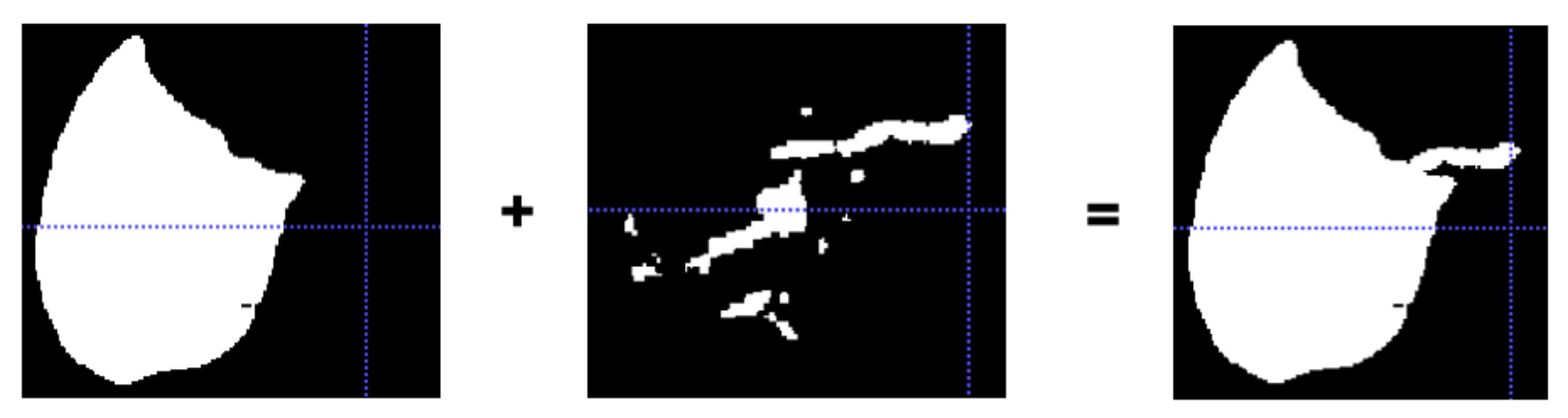
3.6. Masking
To reduce the search space of the 3D U-net, the liver region of interest (ROI) is obtained using the U-net model [
35,
36]. The liver ROI does not include the inlet of the major liver vessels. So, the hepatic vessel ground truth labels were added to get the final liver mask (
Figure 2). Hessian-based vesselness filters are very sensitive to gradient change. In order to avoid the false positives occurring in the liver borders, the liver is masked in the final step after the application of vessel enhancement filters.
3.7. Evaluation
In order to evaluate the results from the experiments, both quantitative and qualitative evaluations were performed. The quantitative evaluation is based on different evaluation metrics and the qualitative evaluation is based on the visual inspection and comparison analysis between predicted and ground truth segmentation.
3.7.1. Quantitative Evaluation
In order to evaluate the segmentation performance, we have selected five different evaluation metrics. These include spatial overlap-based assessment methods such as DICE, Volume Overlap Error (VOE) and Relative Absolute Volume Difference (RAVD) and distance-based measures such as Average symmetric surface distance (ASSD) and maximum symmetric surface distance (MSSD). Below, we briefly describe these metrics.
3.7.2. Dice Coefficient (DICE)
The Dice coefficient (DICE) is the most commonly used metric for validation in medical image segmentation. It is used to find the overlap between the ground-truth segmentation
and the predicted segmentation
using
where
and the
are the cardinalities of the two sets.
3.7.3. Volume Overlap Error (VOE)
Volume Overlap Error is defined as
where
and
are the volumes of segmented regions in the predicted segmentation and ground-truth segmentation, respectively. A value of zero for VOE corresponds to perfect segmentation.
3.7.4. Relative Absolute Volume Difference (RAVD)
Relative Absolute Volume Difference is another volume-based metric and is defined as the ratio of the absolute difference between two segmentation volumes (predicted and ground-truth) and the volume of ground-truth segmentation
A value of RAVD closer to 0 generally corresponds to better segmentation, whereas a higher value suggests poorer segmentation.
3.7.5. Average Symmetric Surface Distance (ASSD)
Average Symmetric Surface Distance is defined as the average of all the distances from boundary points of the segmented image regions to those in the ground-truth. It is given by the following equation:
where
A and
B represent the predicted and ground-truth surfaces, respectively,
and
are the number of points on each
A and
B, and
is the directed distance between mesh points on
A and
B and is given by
with
being the Euclidean distance. A smaller value of ASSD implies better segmentation results.
3.7.6. Maximum Symmetric Surface Distance (MSSD)
Maximum Symmetric Surface Distance is referred to as the maximum of two directed distances between the regions in the ground-truth and segmented image. Similar to ASSD, a smaller value of MSSD implies better segmentation results. For two finite point sets, MSSD is defined in terms of directed distance
as
3.7.7. Qualitative Visual Evaluation
Qualitative visual inspection and evaluation were performed by the same medical doctor who made initial ground truth segmentations. To review predictions from the 3D U-net, 3D Slicer was used to load the original CT images and ground truth segmentations together with predictions. Firstly, the predictions generated from the different enhancement methods were visually inspected. The continuity of major vessels and main bifurcations, which have great clinical importance understanding inflow and outflow in the liver were mainly focused. Secondly, the under- and over-segmentations by calculating the difference between ground truth and predictions were created. These segmentations were visually inspected and used for HU calculation.
4. Experiments
The three experiments conducted in this work are presented in this section. In the first experiment, the effect of different vesselness filters were compared over unenhanced images. In the second experiment, the effects of gamma correction on vesselness filters were studied. In the third experiment, the effect of the fused/combined filter approach was studied.
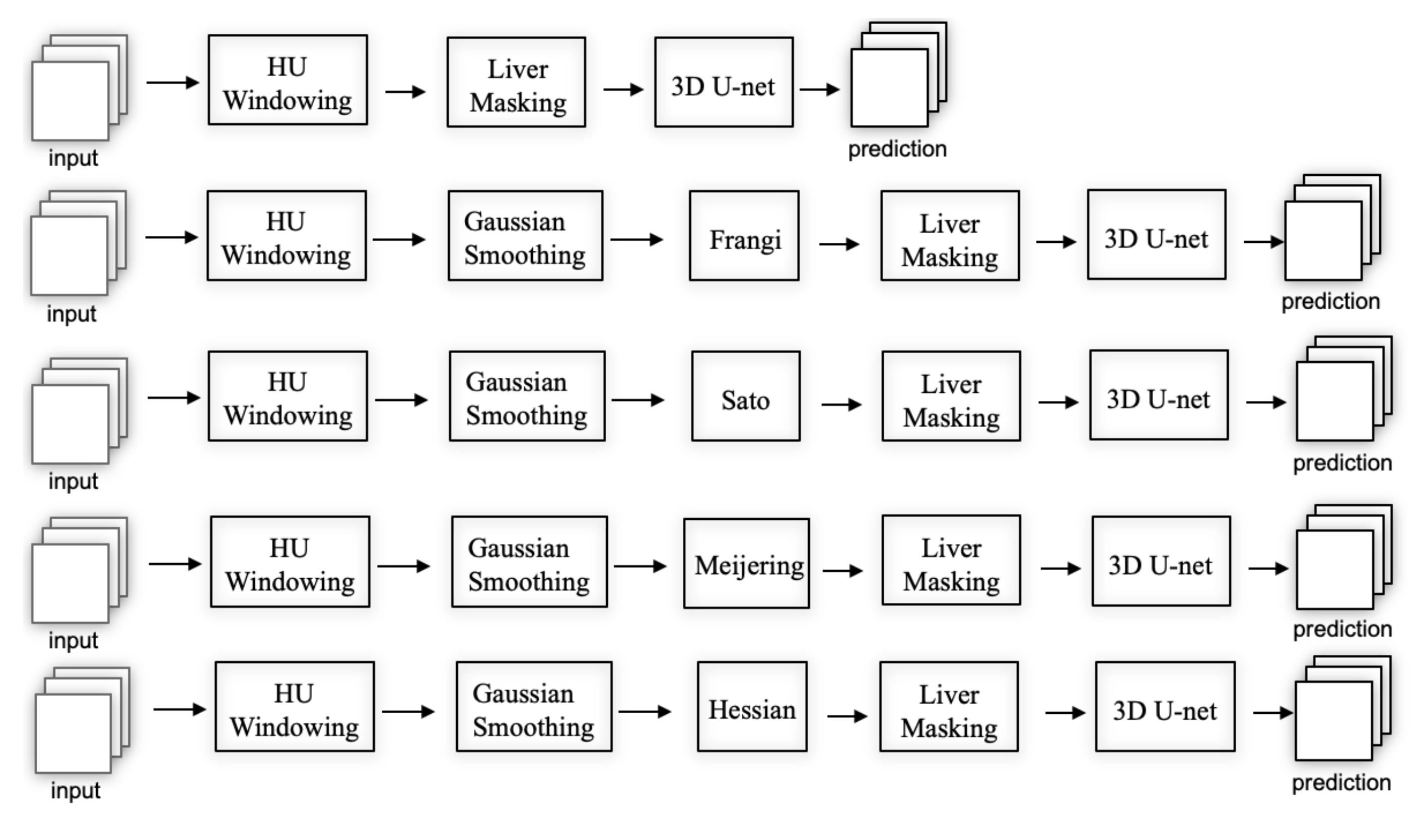
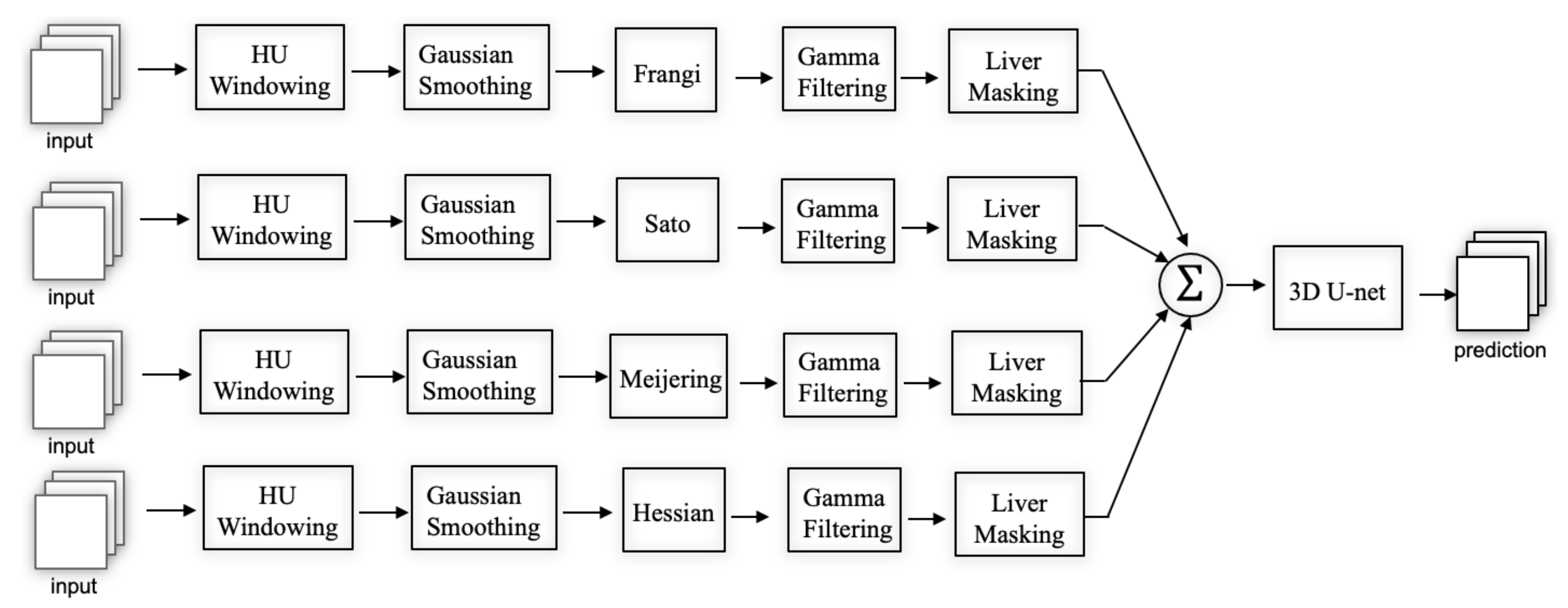
4.1. Experiment 1: Comparison of Different Vesselness Filters
The aim of the first part of the experiment is to compare the results of the unenhanced hepatic vessel segmentation with the segmentation results obtained using different vesselness filters. The second part of the experiment is to compare Frangi, Sato, Meijering and Hessian vesselness filters. For this experiment, a total of five different models were trained. The first model was trained with the images without any vessel enhancement filter. Four other models were trained on Frangi, Sato, Meijering and Hessian vesselness filtered images (
Figure 1d–g), respectively. The workflow of the experiment using these five models is shown in
Figure 3.
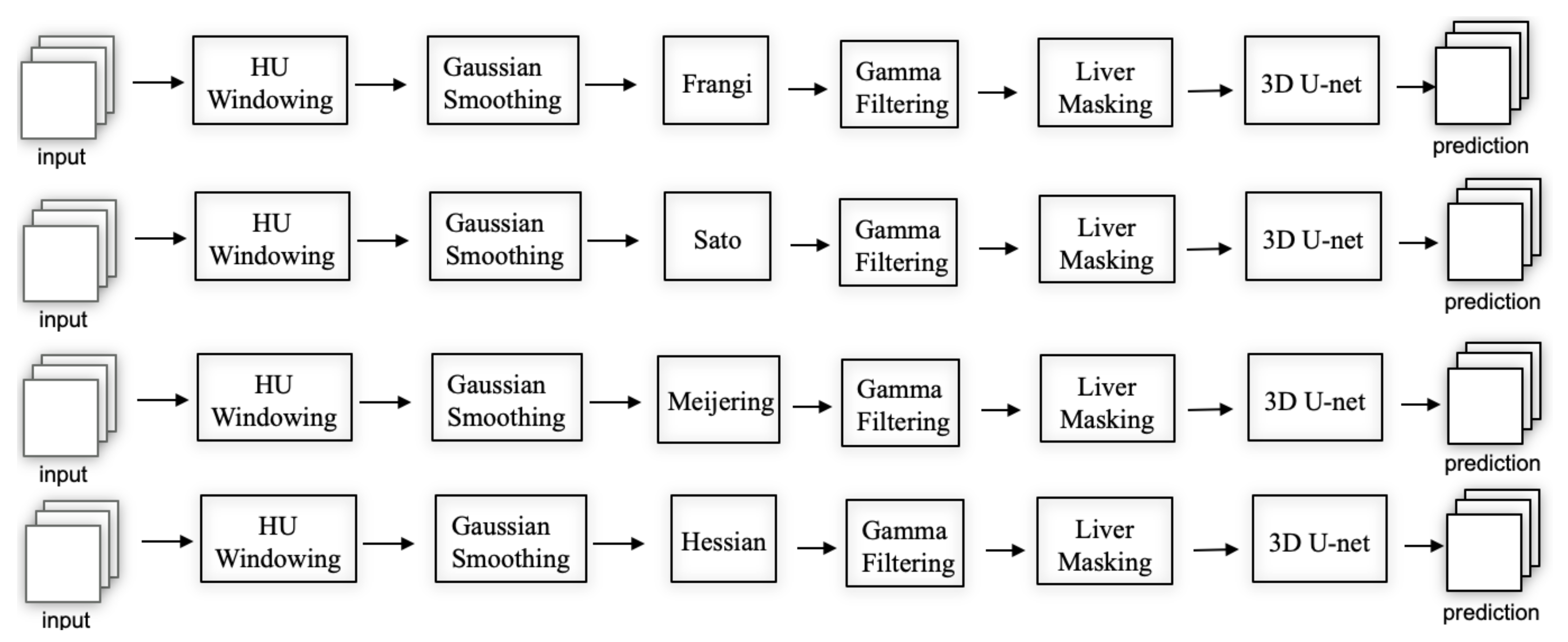
4.2. Experiment 2: Effect of Gamma Correction on Vesselness Filters
In this experiment, the effect of the gamma correction technique on the four vesselness filters was studied. The gamma correction was applied on vesselness filtered images and these images (
Figure 1h–k) were used as an input to the four 3D U-net models (
Figure 4). The segmentation results obtained using gamma-corrected images were compared with the vesselness filtered images without gamma correction.
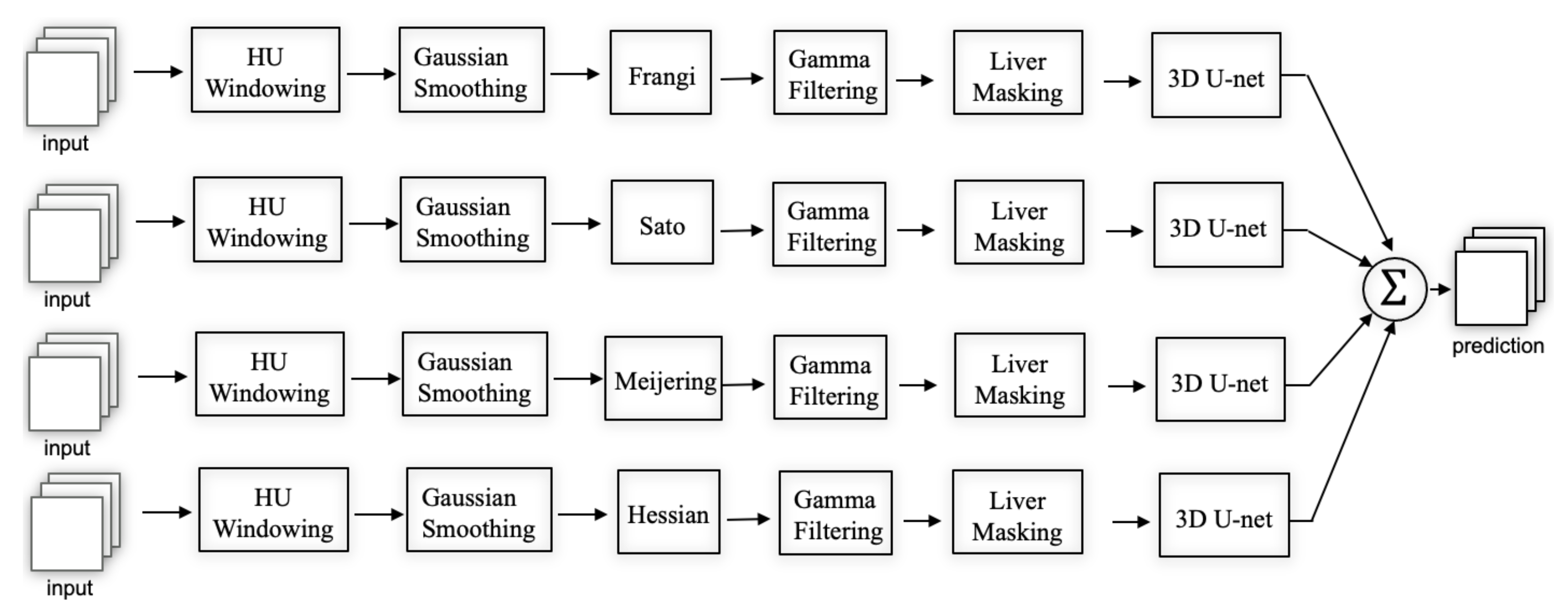
4.3. Experiment 3: Fused Vesselness Filters
In experiment 3, we studied the effect of fused/combined vesselness filters on the individual filters. For this experiment, two different designs were studied. In the first design, the output from the four different filters followed by gamma correction was added channel-wise (
Figure 1l). The U-net model was trained on the vesselness added image (FilterAdded (
Figure 5)). In the second design, the output or the prediction from the four models trained using the four vesselness enhanced gamma-corrected images were added (SegAdded (
Figure 6)) and analyzed. In order to reduce false positives, only the pixels predicted from at least two different filters were considered:
where
,
,
and
are Frangi-, Hessian-, Meijering- and Sato- gamma corrected images respectively.
5. Results
The results from the experiments based on both the technical evaluation and clinical evaluation are analyzed in this section.
5.1. Quantitative Evaluation
In order to evaluate the quality of segmentation, we used the five evaluation metrics presented in
Section 3.7.1 namely DICE, VOE, RAVD, ASSD and MSSD.
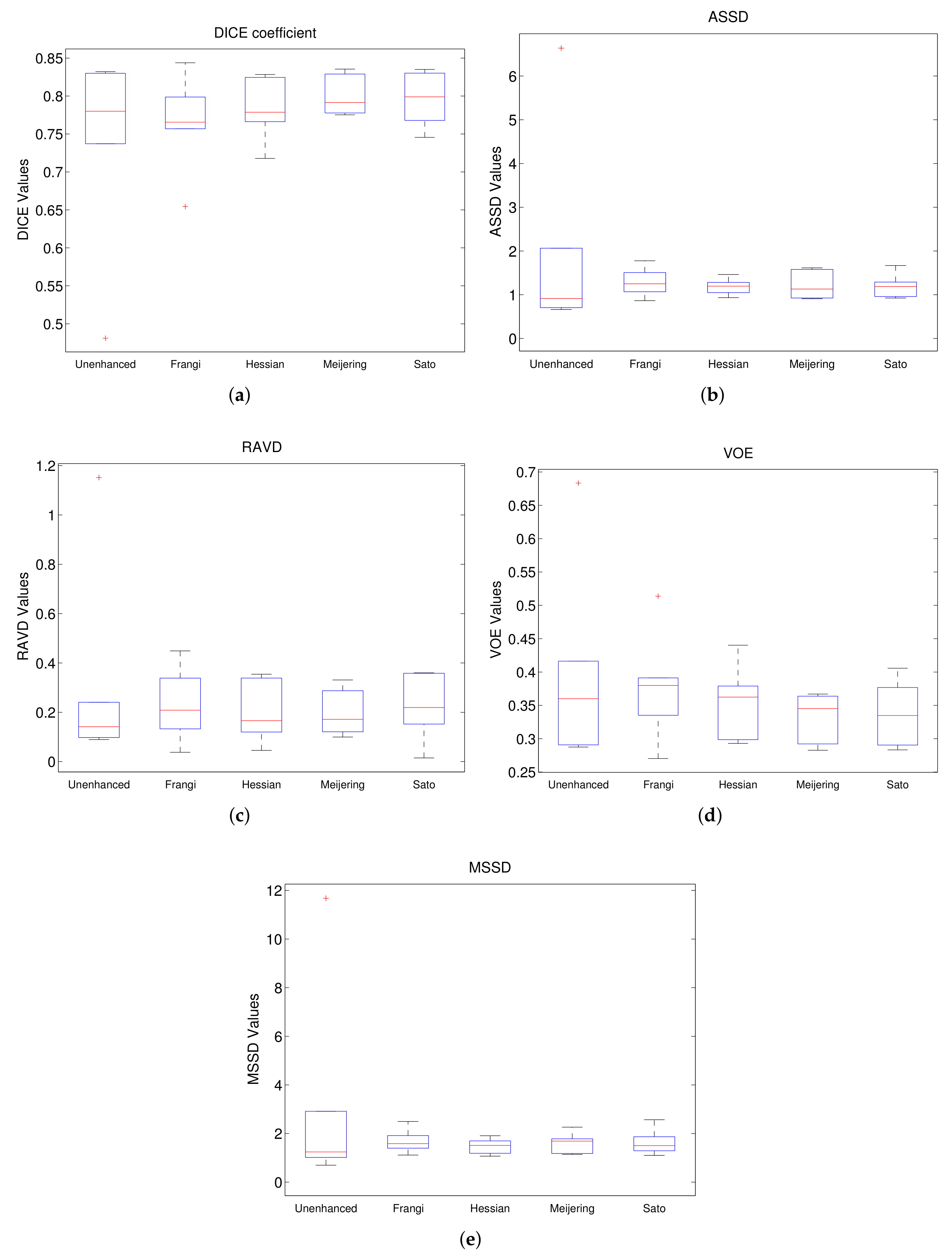
Figure 7 shows the boxplots for each of these metrics for Experiment 1, where the model trained using unenhanced images is compared to those trained with filtered images without Gamma correction. From the DICE boxplot in
Figure 7a, we can observe that the models trained on Sato filtered and Meijering filtered give the best median values and overall spread whereas that based on Frangi gives the worst performance amongst the filtered images. A similar trend is also observed for VOE (
Figure 7d). For ASSD and MSSD (
Figure 7b,e), the median value of the model trained on unfiltered images is the best. This is followed in order by Meijering, Sato, Hessian and Frangi for ASSD and by Hessian, Sato, Frangi and Meijering for MSSD. However, in terms of consistency, all the filtered models can be considered to be superior to the model trained on unenhanced images on the basis of ASSD and MSSD with Hessian being the best, followed by Sato. Finally, for RAVD (
Figure 7c), we also observe the best median value for unenhanced followed closely by Hessian, Meijering, Sato and Frangi. In terms of consistency, all models have a similar spread. However, it is important to note that for each metric unenhanced has an outlier value with a very high deviation which may be attributed to the lack of robustness of this model. Overall, Sato and Meijering can be considered to be the best performing model in Experiment 1 with Hessian as the second-best. This conclusion can also be confirmed on the basis of
Table 1 where the mean and standard deviation of different metrics for each model are presented. From the table, we can see that, amongst the five models compared, Meijering has the best values for all metrics except ASSD, with Sato being the second-best for DICE and VOE, indicating a good overlap between the two volumes. For distance-based metrics, Hessian gives the best mean values which are closely followed by Sato and Meijering. For RAVD, unenhanced has the best mean value, although the value of standard deviation is very high in this case.
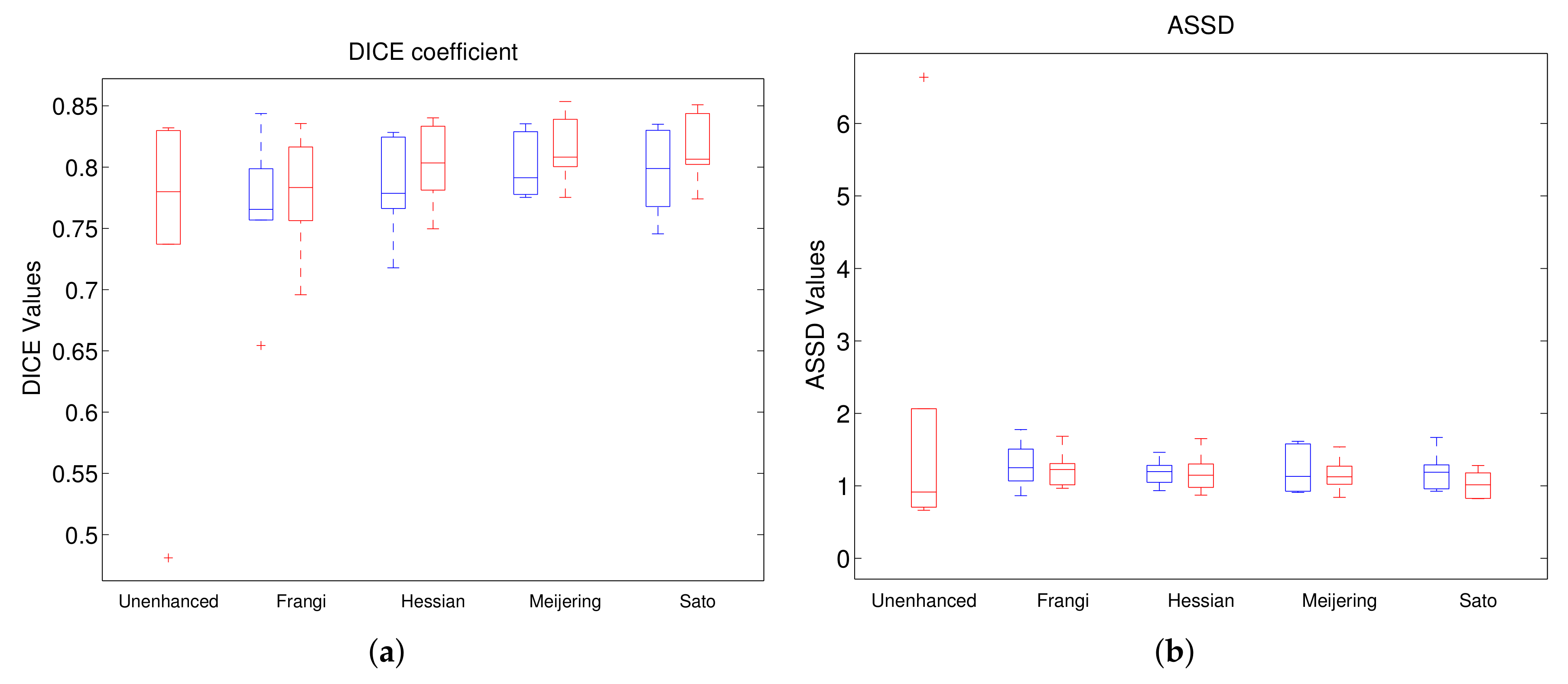
In Experiment 2, we have also included the results of models trained on filtered and gamma-corrected images.
Figure 8 shows the results from this experiment. The left-most box in each boxplot in the figure is that from the unenhanced whereas the remaining boxes are presented in pairs to highlight the differences between the models trained on filtered images with and without gamma correction. In each pair, the boxes in blue represent results from models without gamma correction whereas those in red correspond to those with gamma correction. Overall, we can observe that the models trained with gamma-corrected versions perform much better than their corresponding counterparts with better median values and similar spreads. From among all the methods compared SatoGC has, in general, the best values for all the five metrics followed by MeijeringGC. On the other hand, unenhanced and Frangi give the worst performance from all the methods compared. This holds true also for comparison between mean and standard deviation values as can be seen in
Table 1.
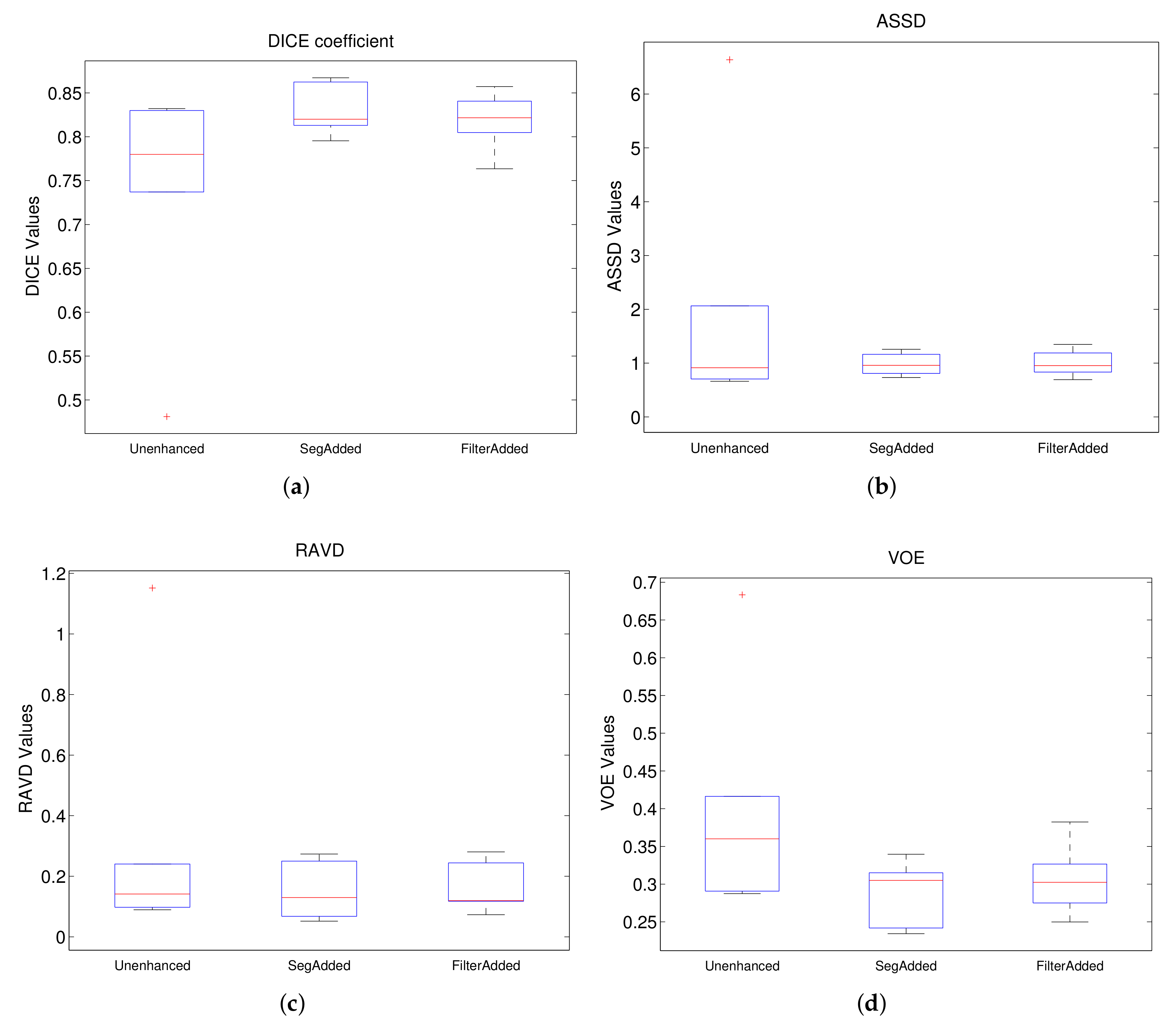
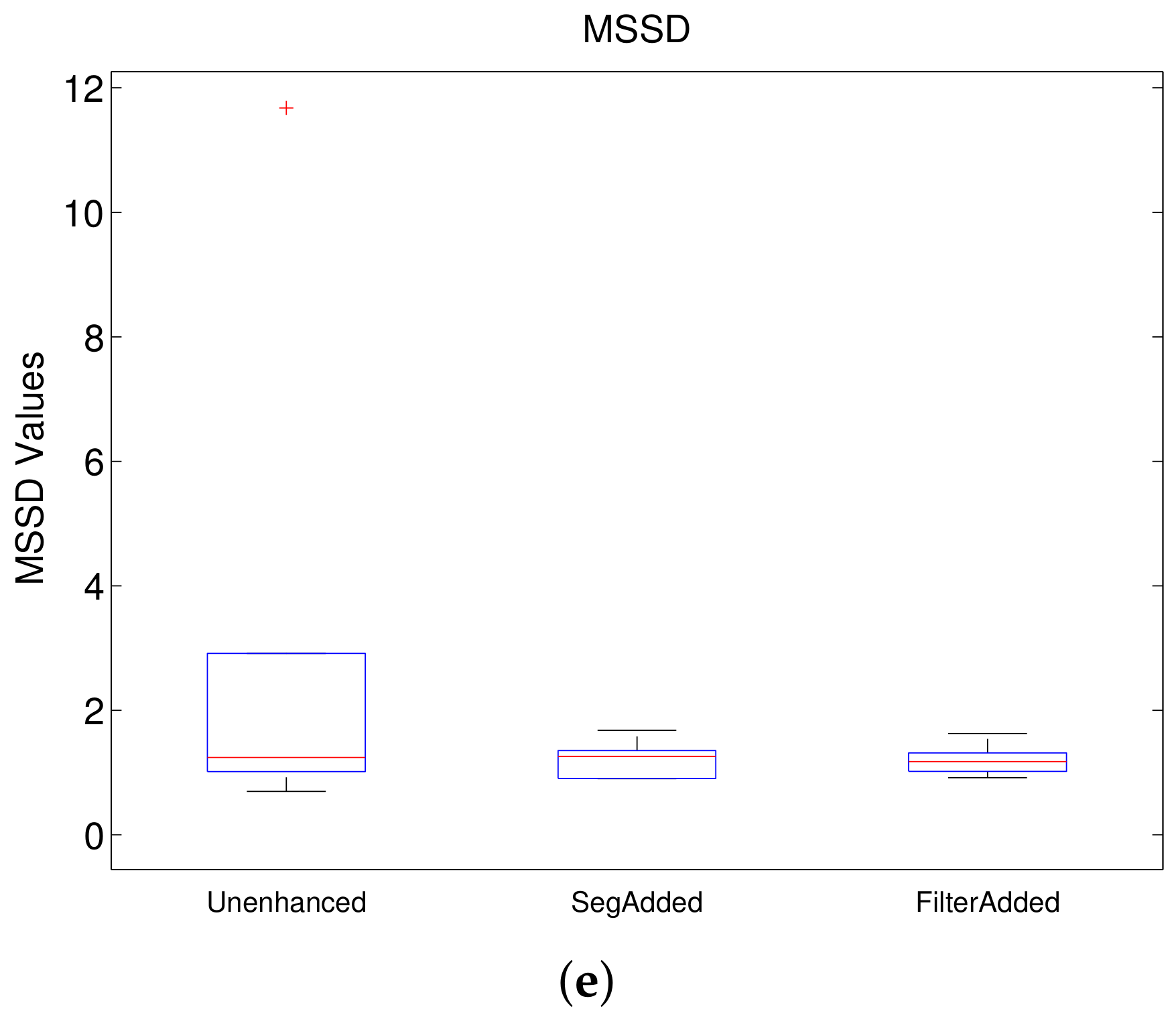
Finally, for Experiment 3, we have compared the results of the two configurations in
Figure 5 and
Figure 6 denoted by SegAdded and FilterAdded with unenhanced. These results are shown in
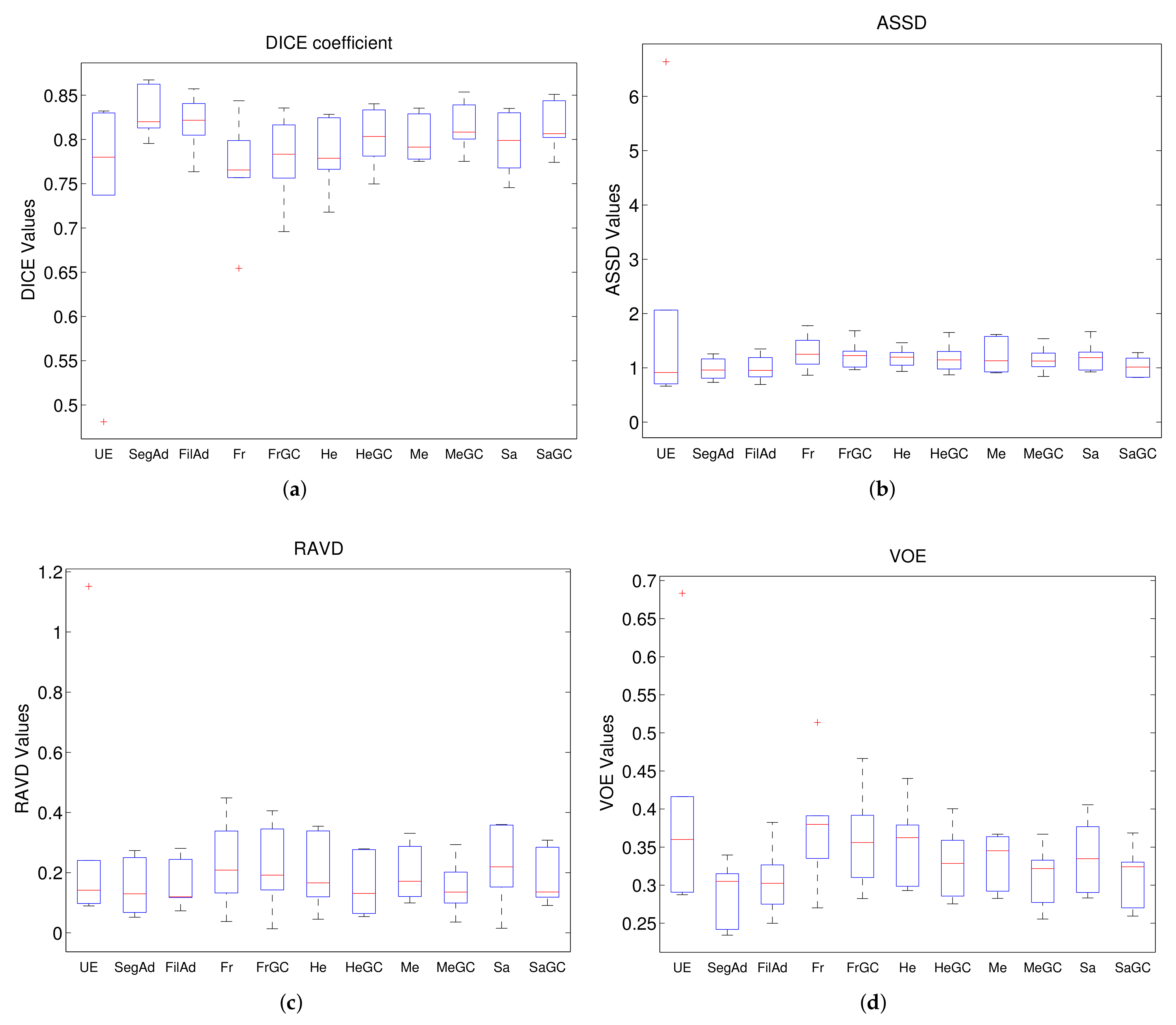
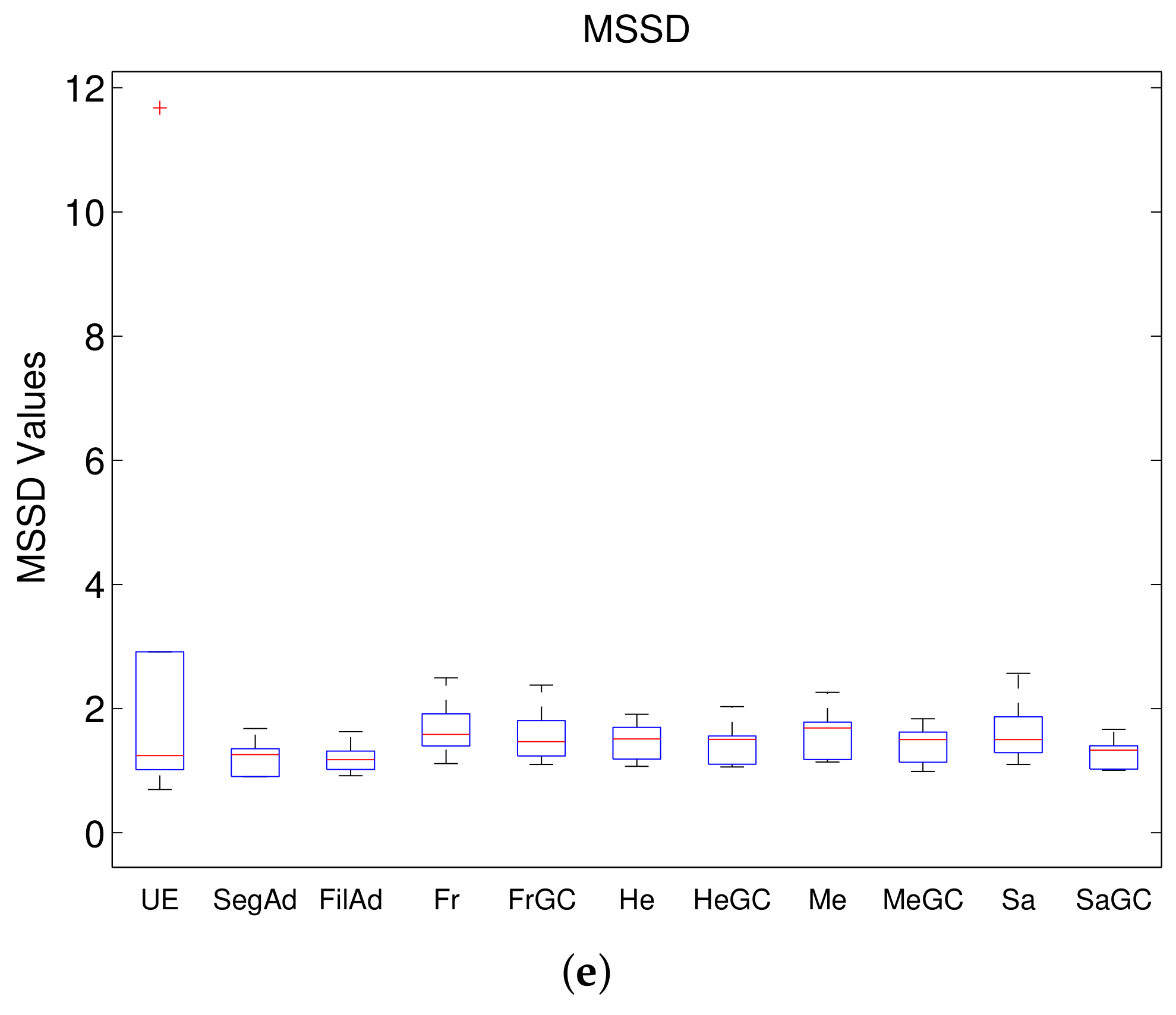
Figure 9. From the results, we can clearly observe that both these methods outperform unenhanced in terms of median values and overall consistency. Both have higher DICE values and lower values for all other metrics depicting better performance. If we compare the performance of the two methods with each other, FilterAdded is the better one with the best median values and a smaller spread for all the metrics. To get an idea of the overall best- and worst-performing methods, we have plotted boxplots of all the methods from the three experiments in
Figure 10. For DICE (
Figure 10a), FilterAdded has the highest median value with a small spreads and hence is the best performing method. This is followed by SegAdded and SatoGC methods. Among the worst-performing are the unenhanced and Frangi. For ASSD (
Figure 10b), the best three are the same but Frangi is the worst in terms of median, whereas unenhanced has the lowest consistency despite a better median value. The same holds true for the MSSD metric (
Figure 10e). Similarly, for RAVD (
Figure 10c) and VOE (
Figure 10d) the best three are FilterAdded, SegAdded and SatoGC, respectively, whereas Frangi is the worst for RAVD and unenhanced is the worst for VOE with a very large spread.
Table 1, displays the mean and standard deviation values from all the filtered and unfiltered models. The values highlighted in bold indicate the best performance for each metric, whereas those in italic are the worst. From the table, we can observe that, as expected, most of the conclusions made based on the boxplots hold true in terms of these values also. In terms of mean and standard deviation values, SegAdded shows the best performance overall with FilterAdded not very far behind. To analyze the significance, we also performed paired t-tests to compare different filtering methods with the two best methods and found improvement using SegAdded to be statistically significant from all of them for majority of metrics. The same results were also found for comparison of all filtered methods with FilterAdded, with the only exception of MeijeringGC and SatoGC, where only values from one of the five metrics were found to be statistically more significant. Hence, in terms of these quantitative results, it can be considered safe to conclude that the SegAdded and the FilterAdded methods are the best whereas the unenhanced and the Frangi give the poorest segmentation results.
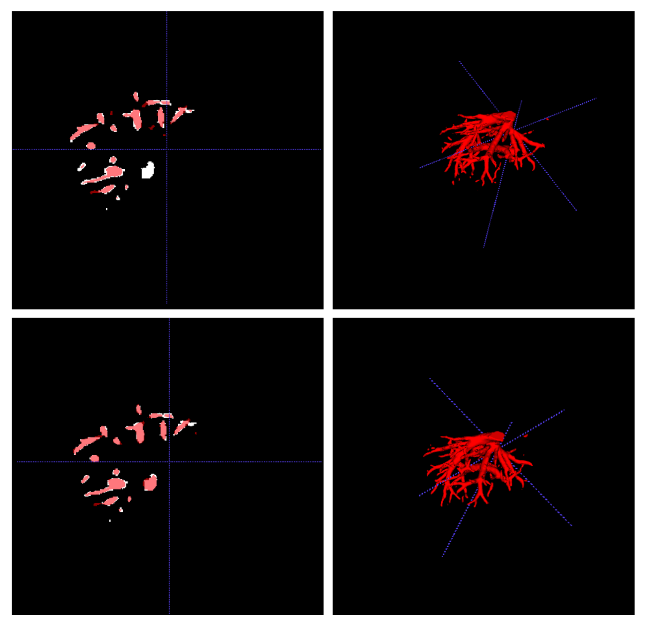
Figure 11 shows the comparison between both the Frangi and SegAdded which has the worst and best mean Dice score respectively.
5.2. Qualitative Evaluation
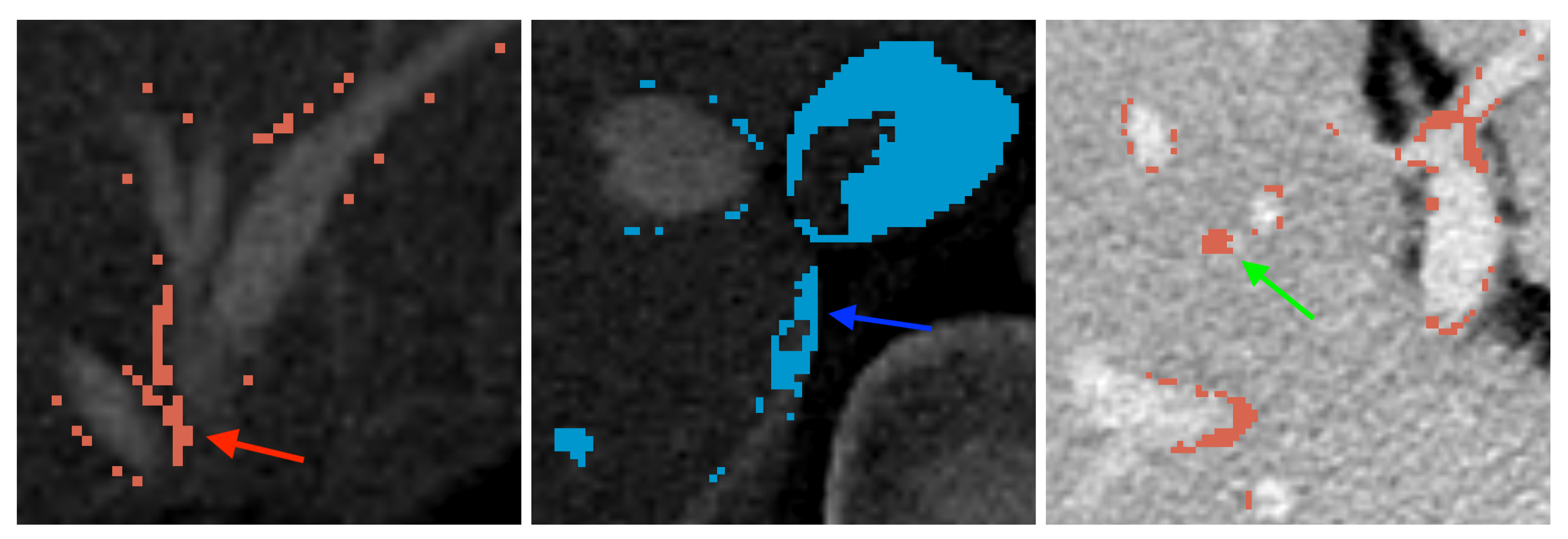
General inspection of the predictions show that results are good as an initial segmentation of the vessels which can be manually corrected, though different fusions and disruptions of vessels are present, examples shown in
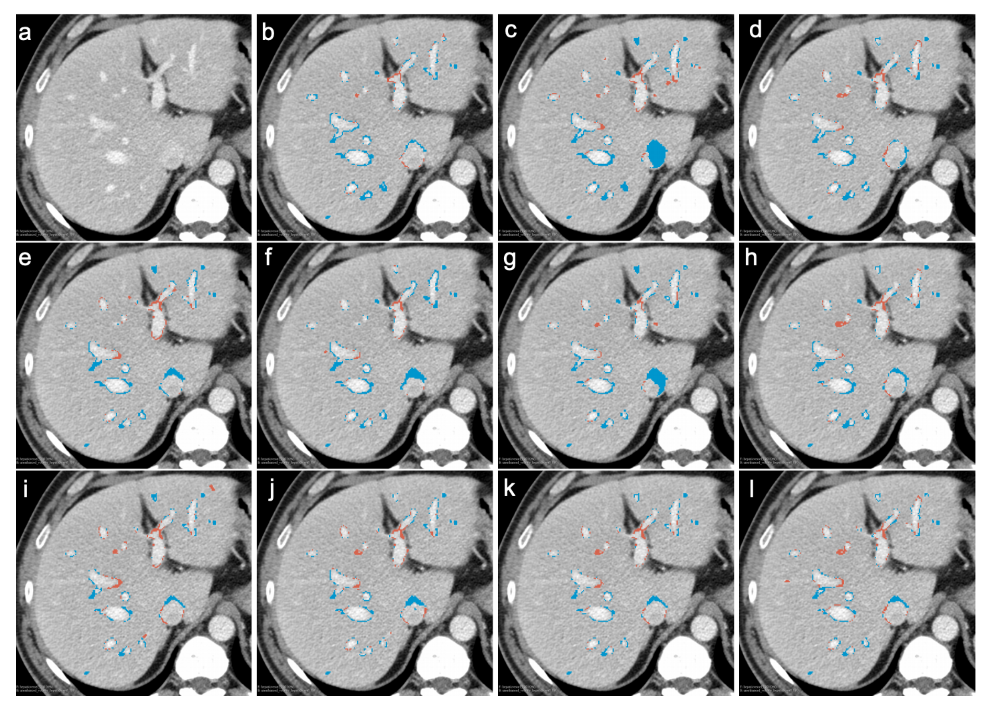
Figure 12. These errors are clearly seen by visual inspection of the inferences together with calculated territories of over- and under-segmentation with examples shown in
Figure 13. Most of the errors are in the edges and borders of vessels. This is supported by values in the CT images showing lower average HU for both over- and under-segmentation, shown in
Table 2.
Overall, the predictions from the deep learning model had an average HU 124.36 ± 26.95 for over-segmentation and 132.59 ± 27.45 for under-segmentation compared to an average 151.91 ± 33.30 for the ground truth. Both over- and under-segmentation capture HU values on average lower than ground truth which indicates that most of the errors are in the edges or additional territories with lower amounts of contrast. In some cases and some slices, predictions in several filtered images captured vessels which were not segmented in the ground truth, examples shown in
Figure 12.
The model trained on unenhanced images generated a visually more “noisy” segmentation with more variations and more extreme errors, shown in
Figure 14. Additionally, the model trained on the unenhanced images had the lowest values of over-segmentation and the highest values of under-segmentation. This can be a sign that these predictions include more of the background in the over-segmentation and misses more high-intensity zones in the under-segmentation.
Overall, visually the SegAdded and the FilterAdded provided a more consistent segmentation of the liver vessels, compared to the other tested methods, and had sometimes advantage of capturing finer details.
6. Discussion
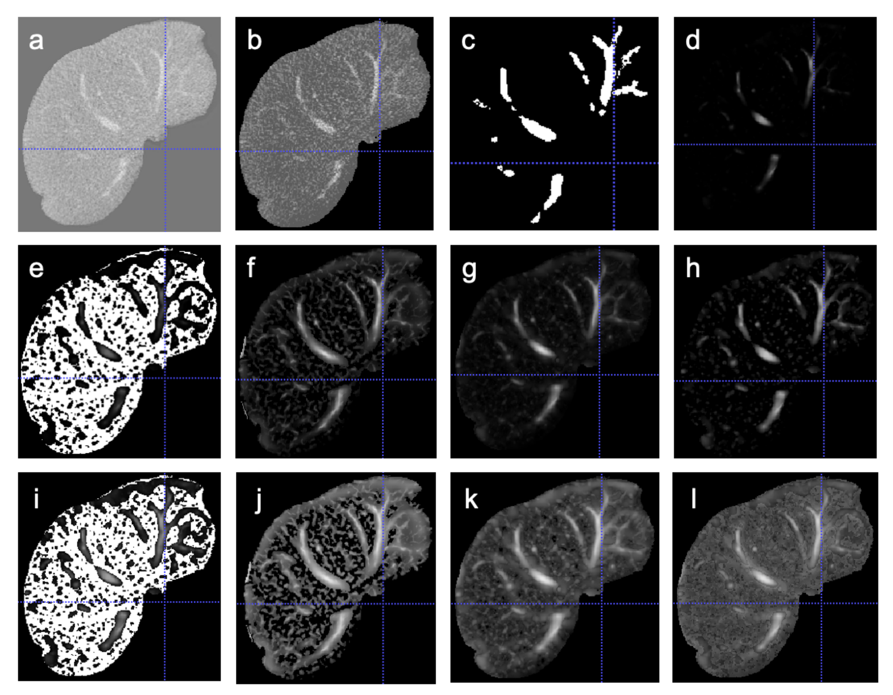
In experiment 1, on comparing the effect of Frangi, Hessian, Sato and Meijering vesselness enhancement filters with the unenhanced images, the model trained on Sato enhanced images seem to perform the best and the model trained on Frangi enhanced images has the worst performance. In addition to the quantitative evaluation, from the
Figure 1, we see that the Sato and Meijering enhanced images seem to capture the vessel information better compared to Hessian and Frangi enhancement. Especially when applying the Frangi vesselness filter, we noticed there is a huge loss of vessel information due to which, the model trained on these images has poorer performance than the model trained on unenhanced images.
In experiment 2, on comparing the effect of gamma correction on Frangi, Hessian, Sato and Meijering vesselness images, we see that the models trained on gamma-corrected images perform better than the ones without gamma correction. Due to gamma correction, the fainter vessel structures in the enhanced images were further enhanced and the models trained on the gamma-corrected enhanced images seem to capture the vessel structure better than the images without gamma correction.
In the final experiment, we studied the effect of fusing all four enhancement filters with gamma correction. In FilterAdded, the FrangiGC, HessianGC, SatoGC and Meijering GC were fused and the model was trained on the fused image. In SegAdded, four different models were trained on FrangiGC, HessianGC, SatoGC and MeijeringGC individually and the segmentation maps from these four models were combined to produce the final segmentation. On comparing FilterAdded and SegAdded, we observed very similar performances with FilterAdded, giving better overall median values and SegAdded giving better mean values. However, the differences between the mean and median metric values were not found to be significant.
On combining the results from all the experiments, the FilterAdded and SegAdded from experiment 3 have the best performance followed by SatoGc. The overall improvement in the performance was found to be statistically significant in terms of the majority of the evaluation metrics for most cases and in terms of at least one metric for MeijeringGC and SatoGC. From the results and the statistical test, we observe that the fused methods have better potential to capture the vessel structures compared to the individual enhancement filters.
Qualitative visual inspection of different results from the methods tested indicates high variability in the vessel edges for all the approaches. Visually, SegAdded and FilterAdded had more consistent predictions with various differences in fine detail depending on the test case. In some slices, vessels were predicted and afterward confirmed by the clinician although defined as oversegmentation because they were not included in the original ground truth. It is important to mention that manual segmentation is a subjective task and is highly user dependent. Therefore ground truth segmentation should not be defined as perfect or complete because there is room for different interpretations and improvements.
Improvement to automatic segmentation might be achieved with the addition of more quality data to train the deep learning model. This work and method provide a solid starting point for vessel segmentation, which can be further worked on using manual correction tools.
7. Conclusions
Automatic segmentation of hepatic vessels is critical for computer-assisted liver surgery, treatment planning and navigation. For the segmentation of complex structures such as liver veins, enhancing the vessel structures makes the segmentation tasks less challenging. In this work, the effects of four different vesselness filters with and without gamma correction have been studied. Additionally, the effect of fused vesselness enhancement over individual filters has been studied. The quantitative analysis of the results in terms of different evaluation metrics from experiments shows that each of the filtered methods improves the segmentation results as compared to those that are unenhanced. Moreover, it was observed that, by applying gamma correction, a statistically significant improvement was achieved in the performance of each filter with SatoGC and MeijeringGC giving better results. Finally, our study showed that both the fused filtered images and fused segmentation give the best results in terms of all the five evaluation metrics with a statistically significant improvement compared to the individual filters with and without Gamma correction. The worst performance was observed for that which was unenhanced and for a model with Frangi (without gamma correction). In addition to that, qualitative evaluation of the deep learning-based segmentations showcase current pitfalls and potential to be used clinically although after extensive manual corrections. To conclude, this work provides an important contribution towards the improvement of the outcomes of the challenging hepatic vessel segmentation task, by making intelligent use of the existing vesselness filters for enhancement in combination with deep learning methods.
In the future, we would like to extend the study to clinical MRI volumes and cross-modality vessel enhancement studies for multi-label vessel segmentation (portal and hepatic vein separated).
Author Contributions
Conceptualization, S.S. and F.L.; methodology, S.S., R.P.K. and F.L.; software, S.S.; validation, S.S., Z.A.K. and E.P.; formal analysis, Z.A.K. and E.P.; labeled dataset creation, E.P.; writing—original draft preparation, S.S., Z.A.K. and E.P.; writing—review and editing, S.S., Z.A.K., E.P., F.L., R.P.K. and B.E.; supervision, F.L. and R.P.K.; project administration and funding acquisition F.L. All authors have read and agreed to the published version of the manuscript.
Funding
This work is supported by H2020-MSCA-ITN Marie Skłodowska-Curie Actions, Innovative Training Networks (ITN) -H2020 MSCA ITN 2016 GA EU project number 722068 High Performance Soft Tissue Navigation (HiPerNav).
Institutional Review Board Statement
The study was conducted according to the guidelines of the Declaration of Helsinki, and approved by the Local and Regional Review Board. This study utilizes a dataset derived from Oslo University hospital OSLO-COMET (Oslo Randomized Laparoscopic Versus Open Liver Resection for Colorectal Metastases Trial). (
ClinicalTrials.gov: NCT01516710).
Informed Consent Statement
Informed consent was obtained from all subjects involved in the OSLO-COMET trial.
Data Availability Statement
Restrictions apply. The data are not publicly available due to privacy or ethical issues.
Conflicts of Interest
The authors declare no conflict of interest.
Abbreviations
| CRC | Colorectal Cancer |
| CNN | Convolutional Neural Networks |
| CLAHE | Contrast Limited Adaptive Histogram Equalization |
| RORPO | Ranking the Orientation Response of Path Operators |
| CT | Computer Tomography |
| MRI | Magnetic Resonance Imaging |
| MRA | Magnetic Resonance Angiography |
| CTA | Computed Tomography Angiography |
| HU | Hounsfield unit |
| FrangiGC | Frangi enhanced image with Gamma Correction |
| SatoGC | Sato enhanced image with Gamma Correction |
| HessianGC | Hessian enhanced image with Gamma Correction |
| MeijeringGC | Meijering enhanced image with Gamma Correction |
| FilterAdded | Filtered images Added |
| SegAdded | Segmentation maps Added |
| ROI | Region of Interest |
| DICE | Dice Coefficient |
| VOE | Volume Overlap Error |
| RAVD | Relative Absolute Volume Difference |
| ASSD | Average Symmetric Surface Distance |
| MSSD | Maximum Symmetric Surface Distance |
References
- Sung, H.; Ferlay, J.; Siegel, R.L.; Laversanne, M.; Soerjomataram, I.; Jemal, A.; Bray, F. Global Cancer Statistics 2020: GLOBOCAN Estimates of Incidence and Mortality Worldwide for 36 Cancers in 185 Countries. CA Cancer J. Clin. 2021, 71, 209–249. [Google Scholar] [CrossRef] [PubMed]
- Van der Geest, L.G.; Lam-Boer, J.; Koopman, M.; Verhoef, C.; Elferink, M.A.; de Wilt, J.H. Nationwide trends in incidence, treatment and survival of colorectal cancer patients with synchronous metastases. Clin. Exp. Metastasis 2015, 32, 457–465. [Google Scholar] [CrossRef] [PubMed]
- Siegel, R.L.; Miller, K.D.; Jemal, A. Cancer statistics, 2016. CA Cancer J. Clin. 2016, 66, 7–30. [Google Scholar] [CrossRef]
- Selle, D.; Preim, B.; Schenk, A.; Peitgen, H.O. Analysis of Vasculature for Liver Surgical Planning. IEEE Trans. Med. Imaging 2002, 21, 1344–1357. [Google Scholar] [CrossRef]
- Kumar, R.P. Fast Blood Vessel Segmentation for Surgical and Interventional Planning and Navigation. 2014. Available online: http://urn.nb.no/URN:NBN:no-46196 (accessed on 3 March 2021).
- Chung, M.; Lee, J.; Chung, J.W.; Shin, Y.G. Accurate liver vessel segmentation via active contour model with dense vessel candidates. Comput. Methods Programs Biomed. 2018, 166, 61–75. [Google Scholar] [CrossRef]
- Shahid, M.; Taj, I. A Robust Retinal Vessel Segmentation using Vessels Location Map and Frangi Enhancement Filter. IET Image Process. 2017, 12. [Google Scholar] [CrossRef]
- Soomro, T.A.; Afifi, A.J.; Ali Shah, A.; Soomro, S.; Baloch, G.A.; Zheng, L.; Yin, M.; Gao, J. Impact of Image Enhancement Technique on CNN Model for Retinal Blood Vessels Segmentation. IEEE Access 2019, 7, 158183–158197. [Google Scholar] [CrossRef]
- Blaiech, A.G.; Mansour, A.; Kerkeni, A.; Bedoui, M.H.; Ben Abdallah, A. Impact of Enhancement for Coronary Artery Segmentation Based on Deep Learning Neural Network. In Pattern Recognition and Image Analysis; Morales, A., Fierrez, J., Sánchez, J.S., Ribeiro, B., Eds.; Springer International Publishing: Cham, Switzerland, 2019; pp. 260–272. [Google Scholar]
- Frangi, A.F.; Niessen, W.J.; Vincken, K.L.; Viergever, M.A. Multiscale vessel enhancement filtering. In Medical Image Computing and Computer-Assisted Intervention—MICCAI’98; Wells, W.M., Colchester, A., Delp, S., Eds.; Springer: Berlin/Heidelberg, Germany, 1998; pp. 130–137. [Google Scholar]
- Kumar, R.P.; Barkhatov, L.; Edwin, B.; Albregtsen, F.; Elle, O.J. Portal and Hepatic Vein Segmentation with Leak Restriction: A Pilot Study. In EMBEC & NBC, 2017; Eskola, H., Väisänen, O., Viik, J., Hyttinen, J., Eds.; Springer: Singapore, 2018; pp. 823–826. [Google Scholar]
- Yang, J.; Lou, C.; Fu, J.; Feng, C. Vessel segmentation using multiscale vessel enhancement and a region based level set model. Comput. Med. Imaging Graph. 2020, 85, 101783. [Google Scholar] [CrossRef] [PubMed]
- Drechsler, K.; Laura, C.O.; Wesarg, S. Hepatic vein segmentation using wavefront propagation and multiscale vessel enhancement. In Medical Imaging 2013: Image Processing; Ourselin, S., Haynor, D.R., Eds.; International Society for Optics and Photonics, SPIE: Bellingham, WA, USA, 2013; Volume 8669, pp. 354–360. [Google Scholar] [CrossRef]
- Jerman, T.; Pernuš, F.; Likar, B.; Špiclin, Ž. Beyond Frangi: An improved multiscale vesselness filter. In Medical Imaging 2015: Image Processing; Ourselin, S., Styner, M.A., Eds.; International Society for Optics and Photonics, SPIE: Bellingham, WA, USA, 2015; Volume 9413, pp. 623–633. [Google Scholar] [CrossRef]
- Kumar, R.; Albregtsen, F.; Reimers, M.; LangÞ, T.; Edwin, B.; Elle, O. 3D Multiscale Vessel Enhancement Based Centerline Extraction of Blood Vessels. In Medical Imaging 2013: Image Processing; International Society for Optics and Photonics, SPIE: Bellingham, WA, USA, 2013; Volume 8669, p. 86691X. [Google Scholar] [CrossRef]
- Lamy, J.; Merveille, O.; Kerautret, B.; Passat, N.; Vacavant, A. Vesselness filters: A survey with benchmarks applied to liver imaging. In Proceedings of the International Conference on Pattern Recognition (ICPR), Milan, Italy, 10–15 January 2021. [Google Scholar]
- Zeng, Y.Z.; Zhao, Y.Q.; Liao, M.; Zou, B.J.; Wang, X.F.; Wang, W. Liver vessel segmentation based on extreme learning machine. Phys. Med. 2016, 32, 709–716. [Google Scholar] [CrossRef] [PubMed]
- Manh Luu, H.; Moelker, A.; Klink, C.; Mendrik, A.; Niessen, W.; van Walsum, T. Evaluation of Diffusion Filters for 3D CTA Liver Vessel Enhancement. In Abdominal Imaging. Computational and Clinical Applications; Yoshida, H., Hawkes, D., Vannier, M.W., Eds.; Springer: Berlin/Heidelberg, Germany, 2012; pp. 168–177. [Google Scholar]
- Phellan, R.; Forkert, N.D. Comparison of vessel enhancement algorithms applied to Time-of-Flight MRA images for cerebrovascular segmentation. Med. Phys. 2017, 44. [Google Scholar] [CrossRef] [PubMed]
- Karuppanagounder, S.; Palanisamy, K. Medical Image Contrast Enhancement based on Gamma Correction. Int. J. Knowl. Manag. e-Learn. 2011, 3, 15–18. [Google Scholar]
- Tiwari, M.; Gupta, B. Brightness preserving contrast enhancement of medical images using adaptive gamma correction and homomorphic filtering. In Proceedings of the 2016 IEEE Students’ Conference on Electrical, Electronics and Computer Science (SCEECS), Bhopal, India, 5–6 March 2016; pp. 1–4. [Google Scholar] [CrossRef]
- Dash, S.; Senapati, M.R. Enhancing detection of retinal blood vessels by combined approach of DWT, Tyler Coye and Gamma correction. Biomed. Signal Process. Control 2020, 57, 101740. [Google Scholar] [CrossRef]
- Zhitao, X.; Xinpeng, Z.; Fang, Z.; Lei, G.; Jun, W.; Long, S.; Liming, C. Diabetic Retinopathy Retinal Image Enhancement Based on Gamma Correction. J. Med. Imaging Health Inform. 2017, 7, 149–154. [Google Scholar] [CrossRef]
- Çiçek, Ö.; Abdulkadir, A.; Lienkamp, S.S.; Brox, T.; Ronneberger, O. 3D U-Net: Learning Dense Volumetric Segmentation from Sparse Annotation. In Medical Image Computing and Computer-Assisted Intervention–MICCAI 2016; Springer: Cham, Switzerland, 2016; Volume 9901, pp. 424–432. [Google Scholar] [CrossRef]
- Litjens, G.; Kooi, T.; Bejnordi, B.E.; Setio, A.A.A.; Ciompi, F.; Ghafoorian, M.; van der Laak, J.A.W.M.; van Ginneken, B.; Sánchez, C.I. A Survey on Deep Learning in Medical Image Analysis. Med. Image Anal. 2017, 42, 60–88. [Google Scholar] [CrossRef] [PubMed]
- Yushkevich, P.A.; Gao, Y.; Gerig, G. ITK-SNAP: An interactive tool for semi-automatic segmentation of multi-modality biomedical images. In Proceedings of the 2016 38th Annual International Conference of the IEEE Engineering in Medicine and Biology Society (EMBC), Orlando, FL, USA, 16–20 August 2016; pp. 3342–3345. [Google Scholar] [CrossRef]
- Fedorov, A.; Beichel, R.; Kalpathy-Cramer, J.; Finet, J.; Fillion-Robin, J.C.; Pujol, S.; Bauer, C.; Jennings, D.; Fennessy, F.; Sonka, M.; et al. 3D Slicer as an image computing platform for the Quantitative Imaging Network. Magn. Reson. Imaging 2012, 30, 1323–1341. [Google Scholar] [CrossRef] [PubMed]
- Van der Walt, S.; Schönberger, J.L.; Nunez-Iglesias, J.; Boulogne, F.; Warner, J.D.; Yager, N.; Gouillart, E.; Yu, T.; The Scikit-Image Contributors. scikit-image: Image processing in Python. PeerJ 2014, 2, e453. [Google Scholar] [CrossRef] [PubMed]
- Adams, J.E.; Mughal, Z.; Damilakis, J.; Offiah, A.C. Radiology. In Pediatric Bone, 2nd ed.; Glorieux, F.H., Pettifor, J.M., Jüppner, H., Eds.; Academic Press: San Diego, CA, USA, 2012; Chapter 12; pp. 277–307. [Google Scholar] [CrossRef]
- Ng, C.C.; Yap, M.H.; Costen, N.; Li, B. Automatic Wrinkle Detection Using Hybrid Hessian Filter. In Computer Vision—ACCV 2014; Cremers, D., Reid, I., Saito, H., Yang, M.H., Eds.; Springer International Publishing: Cham, Switzerland, 2015; pp. 609–622. [Google Scholar]
- Meijering, E.; Jacob, M.; Sarria, J.C.; Steiner, P.; Hirling, H.; Unser, M. Design and validation of a tool for neurite tracing and analysis in fluorescence microscopy images. Cytom. Part A 2004, 58A, 167–176. [Google Scholar] [CrossRef] [PubMed]
- Obara, B.; Fricker, M.; Gavaghan, D.; Grau, V. Contrast-Independent Curvilinear Structure Detection in Biomedical Images. IEEE Trans. Image Process. Publ. IEEE Signal Process. Soc. 2012, 21, 2572–2581. [Google Scholar] [CrossRef] [PubMed]
- Sato, Y.; Nakajima, S.; Shiraga, N.; Atsumi, H.; Yoshida, S.; Koller, T.; Gerig, G.; Kikinis, R. Three-dimensional multi-scale line filter for segmentation and visualization of curvilinear structures in medical images. Med. Image Anal. 1998, 2, 143–168. [Google Scholar] [CrossRef]
- Choudhury, A.K.R. 7—Using instruments to quantify colour. In Principles of Colour and Appearance Measurement; Choudhury, A.K.R., Ed.; Woodhead Publishing: Sawston, UK, 2014; pp. 270–317. [Google Scholar] [CrossRef]
- Bilic, P.; Christ, P.F.; Vorontsov, E.; Chlebus, G.; Chen, H.; Dou, Q.; Fu, C.; Han, X.; Heng, P.; Hesser, J.; et al. The Liver Tumor Segmentation Benchmark (LiTS). arXiv 2019, arXiv:1901.04056.2019. [Google Scholar]
- Pedersen, A. Automatic Liver Segmentation in CT Using Deep Learning. 2020. Available online: https://github.com/andreped/livermask (accessed on 8 December 2020).
Figure 1.
Comparison of different enhancement methods. (a) Original image, (b) HW, (c) Ground truth, (d) Frangi, (e) Hessian, (f) Meijering, (g) Sato, (h) FrangiGC, (i) HessianGC, (j) MeijeringGC, (k) SatoGC, (l) FilterAdded.
Figure 1.
Comparison of different enhancement methods. (a) Original image, (b) HW, (c) Ground truth, (d) Frangi, (e) Hessian, (f) Meijering, (g) Sato, (h) FrangiGC, (i) HessianGC, (j) MeijeringGC, (k) SatoGC, (l) FilterAdded.
Figure 2.
Masking. Liver ROI (left), vessel ground truth (middle), final liver mask (right).
Figure 2.
Masking. Liver ROI (left), vessel ground truth (middle), final liver mask (right).
Figure 3.
Workflow of the unenhanced and different vesselness enhancement approaches.
Figure 3.
Workflow of the unenhanced and different vesselness enhancement approaches.
Figure 4.
Workflow of different vesselness enhancement approaches with gamma correction.
Figure 4.
Workflow of different vesselness enhancement approaches with gamma correction.
Figure 5.
Workflow of the combined vesselness filter output (FilterAdded).
Figure 5.
Workflow of the combined vesselness filter output (FilterAdded).
Figure 6.
Workflow of the combined prediction from different vesselness filters (SegAdded).
Figure 6.
Workflow of the combined prediction from different vesselness filters (SegAdded).
Figure 7.
Comparison of segmentation for unenhanced and different filtered images (red + are outliers). (a) DICE; (b) ASSD; (c) RAVD; (d) VOE; (e) MSSD.
Figure 7.
Comparison of segmentation for unenhanced and different filtered images (red + are outliers). (a) DICE; (b) ASSD; (c) RAVD; (d) VOE; (e) MSSD.
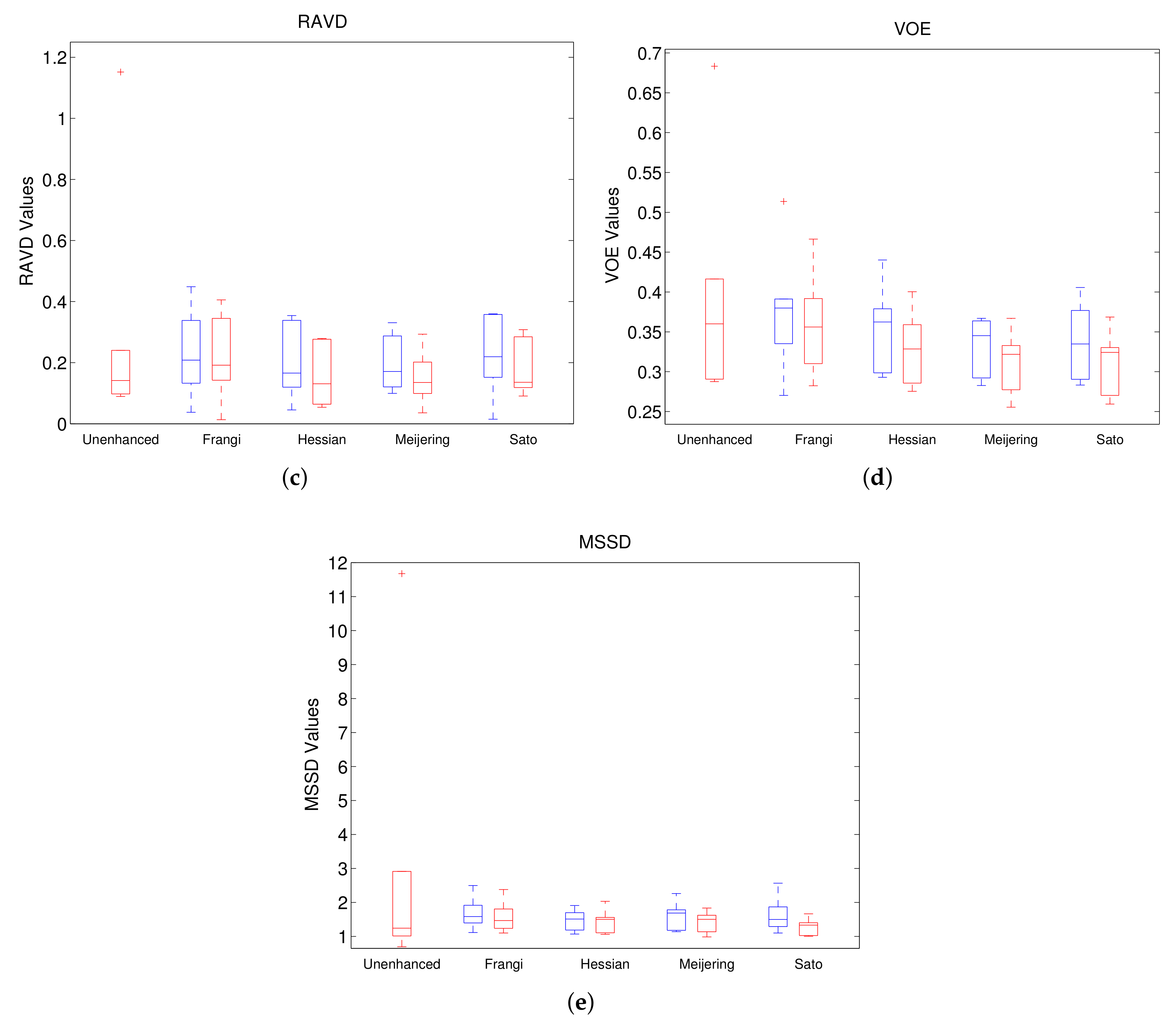
Figure 8.
Comparison of segmentation of unenhanced (first red) and filtered images without (blue) and with (red) Gamma correction. (a) DICE; (b) ASSD; (c) RAVD; (d) VOE; (e) MSSD.
Figure 8.
Comparison of segmentation of unenhanced (first red) and filtered images without (blue) and with (red) Gamma correction. (a) DICE; (b) ASSD; (c) RAVD; (d) VOE; (e) MSSD.
Figure 9.
Comparison of segmentation of filtered images with combination of filters. (a) DICE; (b) ASSD; (c) RAVD; (d) VOE; (e) MSSD.
Figure 9.
Comparison of segmentation of filtered images with combination of filters. (a) DICE; (b) ASSD; (c) RAVD; (d) VOE; (e) MSSD.
Figure 10.
Comparison of all the methods. UE—Unenhanced, SegAd—SegAdded, FilAd—FilterAdded, Fr—Frangi, FrGC—FrangiGC, He—Hessian, HeGC—HessianGC, Me—Meijering, MeGC—MeijeringGC, Sa—Sato, SaGC—SatoGC. (a) DICE; (b) ASSD; (c) RAVD; (d) VOE; (e) MSSD.
Figure 10.
Comparison of all the methods. UE—Unenhanced, SegAd—SegAdded, FilAd—FilterAdded, Fr—Frangi, FrGC—FrangiGC, He—Hessian, HeGC—HessianGC, Me—Meijering, MeGC—MeijeringGC, Sa—Sato, SaGC—SatoGC. (a) DICE; (b) ASSD; (c) RAVD; (d) VOE; (e) MSSD.
Figure 11.
Liver vessel segmentation overlay on ground truth using Frangi enhanced image which has the worst Dice score; 2D slice (top-left) and 3D view (top-right), and SegAdded image which has the best Dice score; 2D slice (bottom-left) and 3D view (bottom-right).
Figure 11.
Liver vessel segmentation overlay on ground truth using Frangi enhanced image which has the worst Dice score; 2D slice (top-left) and 3D view (top-right), and SegAdded image which has the best Dice score; 2D slice (bottom-left) and 3D view (bottom-right).
Figure 12.
Left image—an example of oversegmentation in the borders of the vessels with a vessel fusion in the bifurcation (red arrow). Middle image—undersegmentation disrupting vessel continuity (blue arrow). Right image—an example of a segmented vessel which was not detected and segmented in the ground truth (green arrow).
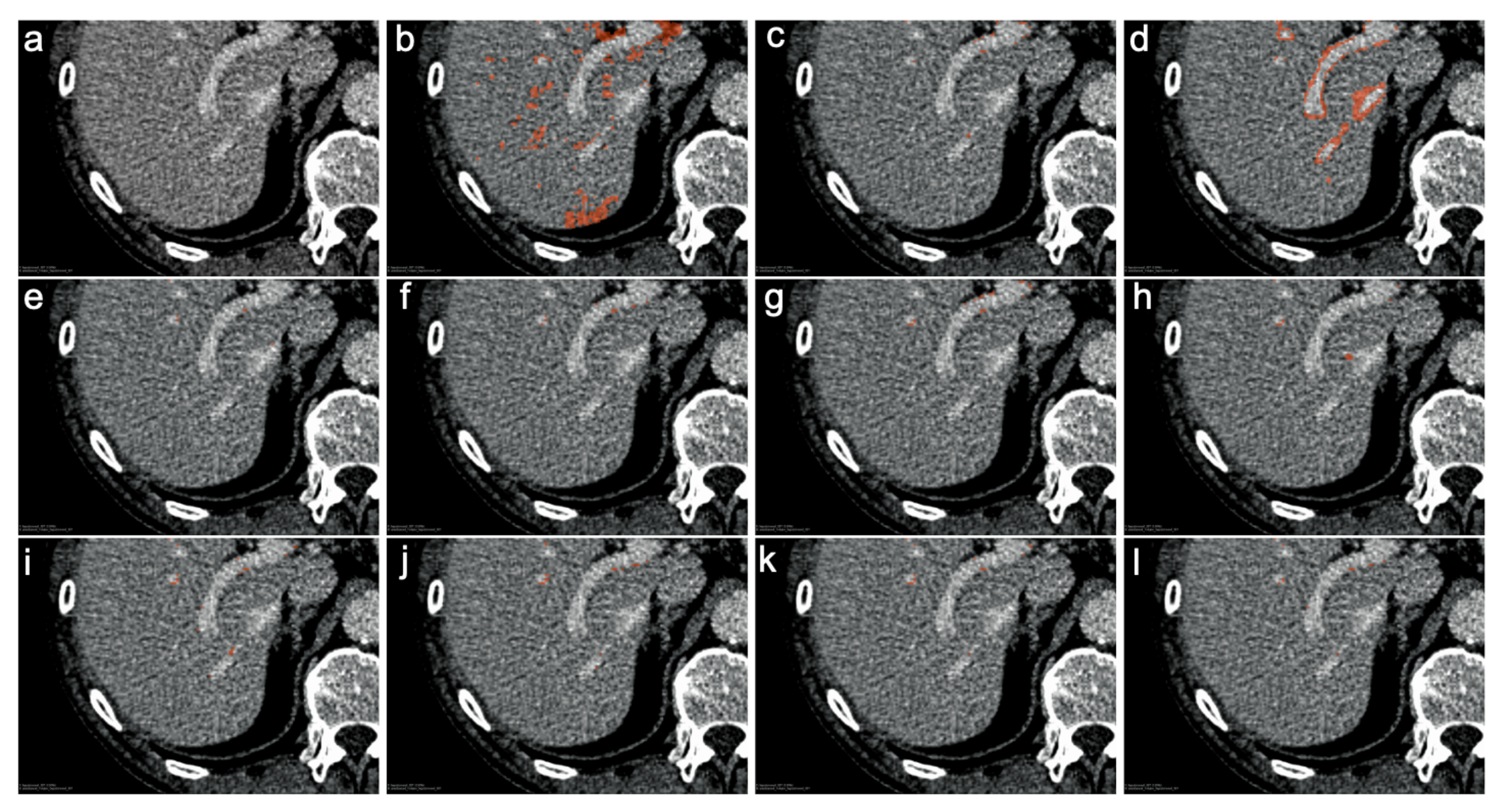
Figure 13.
A slice in the CT images from test data followed by examples of oversegmentation (shown in red) and undersegmentation (shown in blue) from all image enchanchements tested. (a) Original image, (b) Unenhanced, (c) Frangi, (d) Hessian, (e) Meijering, (f) Sato, (g) FrangiGC, (h) HessianGC, (i) MeijeringGC, (j) SatoGC, (k) SegAdded, (l) FilterAdded.
Figure 14.
A slice in the CT images from test data followed by examples of over-segmentation (shown in red) from all image enhancements tested. (a) Original image, (b) Unenhanced, (c) Frangi, (d) Hessian, (e) Meijering, (f) Sato, (g) FrangiGC, (h) HessianGC, (i) MeijeringGC, (j) SatoGC, (k) SegAdded, (l) FilterAdded.
Table 1.
Mean and standard deviation values for Segmentation metrics with different filtering.
Table 1.
Mean and standard deviation values for Segmentation metrics with different filtering.
| Filtering | DICE | ASSD | RAVD | VOE | MSSD |
|---|
| Unenhanced | 0.740 ± 0.121 | 1.982 ± 2.135 | 0.310 ± 0.380 | 0.340 ± 0.136 | 3.132 ± 3.887 |
| Frangi | 0.764 ± 0.057 | 1.285 ± 0.294 | 0.229 ± 0.136 | 0.378 ± 0.073 | 1.683 ± 0.438 |
| Hessian | 0.782 ± 0.037 | 1.186 ± 0.172 | 0.198 ± 0.113 | 0.356 ± 0.050 | 1.481 ± 0.298 |
| Meijering | 0.800 ± 0.024 | 1.213 ± 0.289 | 0.197 ± 0.085 | 0.333 ± 0.033 | 1.624 ± 0.384 |
| Sato | 0.796 ± 0.032 | 1.202 ± 0.246 | 0.221 ± 0.119 | 0.338 ± 0.044 | 1.638 ± 0.491 |
| FrangiGC | 0.778 ± 0.045 | 1.236 ± 0.235 | 0.215 ± 0.131 | 0.360 ± 0.059 | 1.577 ± 0.426 |
| HessianGC | 0.802 ± 0.031 | 1.182 ± 0.254 | 0.156 ± 0.092 | 0.330 ± 0.042 | 1.462 ± 0.325 |
| MeijeringGC | 0.814 ± 0.026 | 1.153 ± 0.216 | 0.150 ± 0.081 | 0.313 ± 0.037 | 1.431 ± 0.288 |
| SatoGC | 0.814 ± 0.026 | 1.022 ± 0.175 | 0.179 ± 0.085 | 0.313 ± 0.037 | 1.294 ± 0.226 |
| SegAdded | 0.830 ± 0.026 | 0.979 ± 0.191 | 0.150 ± 0.084 | 0.290 ± 0.039 | 1.227 ± 0.269 |
| FilterAdded | 0.818 ± 0.031 | 0.995 ± 0.223 | 0.159 ± 0.076 | 0.306 ± 0.043 | 1.206 ± 0.235 |
Table 2.
Average overall HU for test data evaluation with over- and under-segmentation.
Table 2.
Average overall HU for test data evaluation with over- and under-segmentation.
| Label | Overall | Over-Segmentation | Under-Segmentation |
|---|
| Ground truth | 151.91 ± 33.30 | N/A | N/A |
| Unenchanced | 149.60 ± 38.50 | 119.89 ± 40.32 | 135.60 ± 31.90 |
| Frangi | 157.23 ± 32.16 | 123.16 ± 26.28 | 131.86 ± 29.12 |
| Hessian | 155.28 ± 33.89 | 123.25 ± 25.83 | 133.91 ± 26.31 |
| MeijeringGC | 153.08 ± 33.50 | 124.05 ± 25.90 | 132.81 ± 27.73 |
| SatoGC | 154.57 ± 33.32 | 125.42 ± 25.17 | 132.40 ± 26.16 |
| FrangiGC | 157.04 ± 32.03 | 124.71 ± 26.05 | 131.32 ± 29.05 |
| HessianGC | 153.78 ± 33.94 | 123.96 ± 25.11 | 133.67 ± 25.95 |
| Meijering | 154.77 ± 33.40 | 124.13 ± 26.36 | 133.05 ± 27.60 |
| Sato | 156.17 ± 33.66 | 128.31 ± 25.39 | 129.84 ± 26.40 |
| SegAdded | 153.85 ± 33.29 | 126.06 ± 24.82 | 131.61 ± 25.96 |
| FilterAdded | 154.04 ± 33.59 | 125.05 ± 25.25 | 132.41 ± 25.84 |
| Publisher’s Note: MDPI stays neutral with regard to jurisdictional claims in published maps and institutional affiliations. |
© 2021 by the authors. Licensee MDPI, Basel, Switzerland. This article is an open access article distributed under the terms and conditions of the Creative Commons Attribution (CC BY) license (https://creativecommons.org/licenses/by/4.0/).


 ,
, 


