LSTM Networks for Overcoming the Challenges Associated with Photovoltaic Module Maintenance in Smart Cities

Abstract

Predictive maintenance is a field of research that has emerged from the need to improve the systems in place. This research focuses on controlling the degradation of photovoltaic (PV) modules in outdoor solar panels, which are exposed to a variety of climatic loads. Improved reliability, operation, and performance can be achieved through monitoring. In this study, a system capable of predicting the output power of a solar module was implemented. It monitors different parameters and uses automatic learning techniques for prediction. Its use improved reliability, operation, and performance. On the other hand, automatic learning algorithms were evaluated with different metrics in order to optimize and find the best configuration that provides an optimal solution to the problem. With the aim of increasing the share of renewable energy penetration, an architectural proposal based on Edge Computing was included to implement the proposed model into a system. The proposed model is designated for outdoor predictions and offers many advantages, such as monitoring of individual panels, optimization of system response, and speed of communication with the Cloud. The final objective of the work was to contribute to the smart Energy system concept, providing solutions for planning the entire energy system together with the identification of suitable energy infrastructure designs and operational strategies.

1. Introduction

At the moment, we are witnessing major technological developments that make cities smarter in each and every one of their processes. As cities strive to become “smart”, we cannot lose sight of importance of using renewable energies to achieve the cities’ goals. To provide intelligence to the processes, it is necessary to make use of the industry 4.0 paradigm, known as the ”fourth industrial revolution”, which primarily involves the use of IoT (Internet of Things) on interconnected facilities where a large volume of data is collected and processed by Big Data and Machine Learning (ML) techniques [1]. The renewable energy sector is in need of technological solutions capable of perfectly optimizing and integrating processes in the smart city ecosystem by reducing costs and enabling a truly effective and competitive deployment model. For these reasons, the application of novel methods is needed which use a series of smart renewable energy strategies that combine actions in all the energy sectors [2]. Given that photovoltaic (PV) systems are the cheapest source of electricity in sunny locations, we are witnessing significant investment in PV infrastructures and their rapid deployment around the world. However, the outdoor degradation processes are a cause of uncertainty for PV community regarding the reliability and long-term performance of PV modules [3]. The main motivation of this work is to solve the problem of predicting PV energy in solar panels, taking into account the problems associated with the degradation phenomenon in PV modules throughout their lifetime. As solar panels operate in the outdoors, PV modules experience significant performance loss which must be taken into account when performing predictive maintenance and process monitoring. This article’s main focus is predictive maintenance on solar panels. We are in a time of change where energy from fossil fuels are no longer the primary source of energy, and renewable sources, such as solar energy, are much more relevant. Leaman focuses on the benefits of solar energy [4], analyzing its impact and growth in the U.S. in recent years. In 2014 alone, the solar energy industry created more jobs than the big technology companies, such as Apple, Google, Facebook, or Twitter, combined. Moreover, it has come at a crucial time in the energy economy where the rise in electricity prices is not ceasing. Making this type of energy operational is one of the reasons why we are looking for a reduction in the costs of maintaining these facilities. The main novelty of this article lies in the application of an improved model for detecting degradation in PV modules based on Long Short-Term Memory (LSTM) Networks, as well as the proposal of an architecture based on Edge Computing that allows for its operational and scalable implementation. Table 1, below shows the list of abbreviations used in this paper.

Table 1. List of abbreviations.

Abbreviation	Full Form
DKASC	Desert Knowledge Australia Solar Center
ENNs	Echo-State Neural Networks
IoT	Internet of Things
LSTM	Long Short-Term Memory
MAE	Mean Absolute Error
MQTT	Message Queue Telemetry Transport
ML	Machine Learning
MSE	Mean Square Error
NoSQL	not only SQL
SVM	Support Vector Machines
PV	Photovoltaic
ReLU	Rectified Linear Unit
RMSE	Root Mean Square Error
RMSprop	Root Mean Square Propagation
RNN	Recurrent Neural Network
sMAPE	Symmetric Mean Absolute Percentage Error

The article is structured as follows: Section 2 is a review of the state of the art on predictive maintenance in solar panels. Section 3 describes the proposed solution for solar panel monitoring and fault detection, detailing the methodology. Section 4 outlines the conducted case study and its results. Moreover, in this section, the architecture based on Edge Computing is proposed. Finally, in Section 5, the conclusions and future lines of research are presented.

2. Related Works

Among the models that effectively detect failures in photovoltaic (PV) modules, there are architectures that apply predictive methods accompanied by the monitoring of systems in real time and the use of mathematical heuristics to detect abnormal behavior. There are architectures, such as the Edge Computing architectures [5,6], which improve communication with the cloud and relieve computation load by doing the calculations directly on the node. This technique has many benefits, and its standardization is described further on in this article.

Among the algorithms used, it should be noted that most are specific solutions to a given problem using probabilistic models [7,8,9]. As they are specific solutions, they cannot be adjusted to the particularity of each case, which means that they fall behind other types of solutions. Other algorithms to take into account are neural networks and Support Vector Machines (SVM) [10,11,12]. Neural networks have been widely used in recent years, particularly those that are convolutional [13,14,15]. In terms of image recognition [16,17,18,19], the research has focused on two different aspects. One focuses on cloud recognition as a means of predicting the output power of the PV module and the other on the recognition of hot spots or breaks in the panels through images captured by a drone or similar. However, these studies have been discarded as a reference for this proposal because very specific resources are needed, and they are beyond the scope of this study.

The following studies are considered of great interest for this research since they have many points in common with the approach presented here: References [5,11,14,15,20,21,22,23].

Among the methodologies that have been studied there are those that predict the PV power generated by solar modules. In Reference [22], the authors build a predictive algorithm that is capable of predicting the output power of a panel through weather data predictions. As a result, they obtained the best configuration of a neural network, Long Short-Term Memory (LSTM), through statistical metrics, such as mean square error, mean absolute error, etc. In addition, it makes predictions 24 h ahead. Another very similar study is the one proposed in Reference [14], but, in this case, the predictor was based on a convolutional network. They obtained a system to predict consumption peaks in housing communities through wind and solar predictions. When comparing the average error of the square root of the solar predictions, they obtained a superior performance of 7.6% with respect to other studies. However, the cited works do not apply any method of failure prediction.

Another methodology that has been studied is failure analysis as proposed in Reference [20]. It uses a time window of the output power of the PV modules. The temporal curve is then classified either as a correct operation or a specific failure. Given that there were N panels, the worst result that could be obtained is $2N-1$ failure. One of the strengths of this methodology is its ability to detect failures in specific parts of the solar module array. Another approach to consider is the monitoring of solar panels through a neural network, as in Reference [21]. In this study, the authors obtained a power predictor with a network in which precision was not less than 98% and a difference of less than 0.02 between the real value and the predicted value. This difference allowed them to detect degradations in the solar panels and their malfunctioning. Specifically, the work seeks solutions to a problem of regression, focused on time series. To make this prediction, models that can take advantage of time information are usually used. In machine learning, one of the most known models when dealing with time series and making predictions are recurrent neural networks (RNNs). Echo-State Neural Networks (ESNs), is also based on, the projection of a RNN to model the temporal dependencies of the data. They could be of great interest for the problem posed here, since they have demonstrated good performance in time series prediction in solar energy solutions [24,25,26].

Finally, the above studies do not apply their research to a decentralized architecture. However, Reference [5] proposed an architecture where different IoT nodes are monitored. As a result, the authors obtained a year-long analysis of the performance of the solar panels, where highest power production peaks occurred in September and October. They also observed the lowest production in May and March. The biggest problem with this architecture is that it does not implement any automatic learning algorithm to improve the performance of the station. Despite this, the case study is valuable because it describes the deployment of an IoT-based architecture where Edge Computing can be used to reduce latency times and data traffic in communications.

3. Methodology

The present study is a methodological proposal for predictive maintenance involving the elaboration of a system capable of solving a time series problem. Time series problems consist of the study of repetitive patterns over time. Thus, values are determined in the near future and make it possible to make decisions accordingly. It is based on the regression problems, but there are some differences, such as:

• The variables are time-dependent and, therefore, do not comply with all the observations being independent.
• It shows trends of a seasonality, growth, or decrease.

A proposed system capable of obtaining the weather forecast and using it to predict the output power of the solar modules. To this end, the LSTM networks are used, which are described in detail in Section 3.1. Finally, a confidence interval is calculated in real time, and it makes it possible to determine degradations in PV systems, which is described in detail in Section 3.2.

3.1. Definition of LSTM Networks

Long Short-Term Memory (LSTM) networks [27] are an adaptation of RNNs, in particular the change is focused on the hidden layer of the network. This hidden layer is called the LSTM cell, which is made up of three gates, one input, one output, and one override that controls the data flow of the network. In Figure 1, the general scheme of the cell that constitutes the LSTM networks is illustrated. Consider an instant of time t with an input $X_t$, the output of the hidden layer $H_t$, and its previous output $H_{t-1}$, which results in the input state being ${\tilde{C}}_t$, the output state $C_t$ and the previous state $C_{t-1}$. Besides, the gate states take the values of $i_t$, $f_t$, and $o_t$. It should be noted that the values $C_t$ and $H_t$ are propagated through the network, as shown in the scheme.

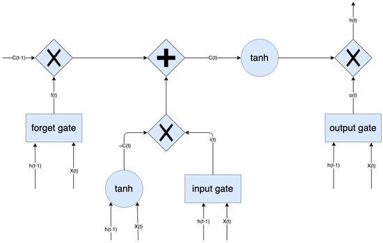
Figure 1. Scheme of a Long Short-Term Memory (LSTM) cell.

To obtain these two values, a series of equations are required. First, states of the three doors and the state of the cell input must be calculated:

$$i_t=\sigma (W_1^i·x_t+W_h^i·h_{t-1}+b_i)\mathrm{Input\; gate},$$

(1)

$$f_t=\sigma (W_1^f·x_t+W_h^f·h_{t-1}+b_f)\mathrm{Forget\; gate},$$

(2)

$$o_t=\sigma (W_1^o·x_t+W_h^o·h_{t-1}+b_o)\mathrm{Output\; gate},$$

(3)

$${\tilde{C}}_t=tanh(W_1^C·x_t+W_h^C·h_{t-1}+b_C)\mathrm{Cell\; entrance},$$

(4)

where $W_1^i$, $W_1^f$, $W_1^o$, $W_1^C$ are the arrays of weights that connect $X_t$ to the three gates and the cell entrance, $W_h^i$, $W_h^f$, $W_h^o$, $W_h^C$ are the weight matrices that connect $h_{t-1}$ to the three gates and the cell entrance, $b_i$, $b_f$, $b_o$, $b_C$ are the bias terms of the three gates and the cell entry, $\sigma$ represents the function $\frac{1}{1+exp(-x)}$, and $tanh$ represents the hyperbolic tangent function $\frac{exp\left(x\right)-exp(-x)}{exp\left(x\right)+exp(-x)}$. Secondly, the output state of the cell is calculated:

$$C_t=i_t·{\tilde{C}}_t+f_t·C_{t-1},$$

(5)

where $i_t$, $f_t$, ${\tilde{C}}_t$, $C_t$, $C_{t-1}$ has the same dimension. Thirdly, the output of the hidden layer is calculated:

$$h_t=o_t·\tanh \left(C_t\right),$$

(6)

The output of the cell is defined as:

$${\tilde{x}}_{t+1}=W_2·h_t+b,$$

(7)

where $W_2$ is the weighting array between the input layer and the output layer, and b is the bias of the output layer.

The size of the window should be taken into account since not having an infinite history limits the window of the network. Historical data go through the whole network, changing its states to obtain the desired prediction.

3.2. System Description

This subsection outlines the network configuration used in the study to develop the power predictor. The design of the neural network was based on trial and error until the best configuration has been obtained that provided the best solution to the problem. The structure can be seen in Figure 2, which contains the following characteristics:

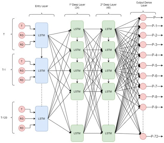
Figure 2. Outline of the proposed LSTM network.

• In the first layer, the number of times to be passed and the number of parameters that form it are specified. In the design, it was specified that it would receive 120 instants of time and three input parameters.
• Two hidden layers are defined with 24 and 48 neurons in which function of activation is ReLU (rectified linear unit). This activation function is the most used in the recurrent neural network (RNN), hence its choice.
• The dense layer with 72 neurons was used as an output in order to obtain the 72 predictions that would form the future window.

The design of the network was based on trial and error [28], until finding the best configuration that encompasses the problem. For the layout of the LSTM network, the TensorFlow library in Python was used. This library allows to handle the Keras module, capable of designing neural networks with a high level of complexity. The training flow of the proposed model involved the manual tunning of the model hyperparameters to boost performance by simple training, validation and test split. The training data are split into 70% training data and 30% validation data (24,283 inputs). On the basis of the regression problem, the loss function that was used was the Mean Square Error (MSE). The performance of the training model is evaluated on the basis on various metrics, including RMSE, MAE, and MSE, detailed in Section 4.1.

On the one hand, the gradient descent algorithm was defined. The Adam algorithm [29] was used, characterized by its notably decreasing learning rates. On the other hand, the number of times specified for the training was 50, and the size of the lots was 120.

Once the network was trained, a prediction window was obtained as a result. The objective of these prediction windows was to analyze the possible anomalies in the PV module. The real power produced by the panel is compared with the power predicted by the neural network. The confidence margins are calculated as those used in the reference article [21], being established on a 10% deviation of the real value from the upper and lower confidence limit. If the predicted value of the network is outside these margins, it is considered that the module may have entered a degradation process. This does not mean that the module is broken, but its operation is anomalous and could become a more serious fault in the future.

$$P_{network}>P_{real}\times 1.1\mathrm{Exceeds\; the\; superior\; limit},$$

(8)

$$P_{network}<P_{real}·0.9\mathrm{Below\; the\; lower\; limit},$$

(9)

where $P_{network}$ is the value obtained by the neural network, and $P_{real}$ is the real power value of the PV panel.

4. Case Study

Subsequently, a case study has been conducted to test the functioning of the neural network and to evaluate its performance.

In the case study, the data provided by the DKASC (Desert Knowledge Australia Solar Center) were used [30], from the Alice Sprint project located in Australia. The selected station is number 25, which was installed in 2016. It belongs to the Hanwha Solar brand with polycrystalline silicon technology. In Table 2, the main characteristics can be observed.

Table 2. Information on the main characteristics of the solar module.

Name	Value
Array Rating	5.83 kW
Panel Rating	265 W
Number of Panels	22
Panel Type	HSL 60S
Array Area	36.74
Inverter Size/Type	SMA SMC 6000A
Installation Completed	Saturday, 2 July 2016
Array Tilt/Azimuth	Tilt = 20, Azi = 0 (Solar North)

The data set consists of measurements that have been taken every 5 min from July 2016 to February 2020. These data have been recorded in an excel spreadsheet that can be accessed publicly from the organization’s website. The file is made up of twelve columns but the six most important columns were extracted according Reference [21]:

• The variable “Timestamp” is used to group the data set because it represents the instant of time when the data was taken.
• The variable “Rainfall” represents the average precipitation measured in millilitres (mL).
• The variable “ActPower” represents the output power of the solar module, measured in kilowatts (kW), and is the target variable that is predicted.
• The variable “Temperature” represents the temperature that is recorded in the zone measured in Celsius (°C).
• The variable “DiffuseRadation” represents diffuse radiation, that is, radiation that does not directly affect the panel. It is also measured in W/m².

The correlation between the 12 features in the data set is analyzed, shown in Figure 3, with the aim of discarding those that do not contribute knowledge to the model. The main focus was to obtain the output power. It is true that, if the algorithm were to detect clouds, it would make more sense to predict the solar incidence, or, if the model were applied to wind energy, it would have more value than the radiation index. The variable “active energy delivered-received” has been discarded as it represents the energy status of the entire solar station. In the case study, the focus is on a specific station, not on all the solar plants in the park. On the other hand, the variable “Current Phase Average” is the output variable of the panel but is measured in amperes. In future research, it can be taken into account, however not as an input for the model, as it does not provide information. As the variable “Performance Ratio” represents the area of the active board, but does not have knowledge of the relationship between the module arrays, it could not be applied to detect malfunctioning in parts; rather, the overall evaluation of the board as a whole has been chosen. The solar station is located in a warm climate, with no precipitation and no wind, so the variables associated with these phenomena do not provide any knowledge to this particular model (“Wind speed”, “Wind Direction”, “Weather Relative Humidity”, and “Rainfall”). It is proposed to incorporate these variables from data sets created in other geographical points. This would improve the model further.

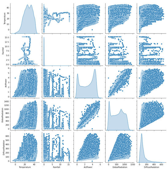
Figure 3. Feature selection: correlation of data set variables.

The most relevant features were those linked to diffuse radiation (RD), global radiation (RG), and temperature (T). These three features were selected as inputs to the neural network, as shown in Figure 2, with the aim of extracting the output window with the output power prediction for the PV panel.

In Figure 4, it is possible to see a representation of the data processed over time. In addition, it can be observed how the radiation values are similar to the power output of the panel, so it was considered that they have a high correlation and can be used by the model. Moreover, the variable that represents the precipitation was eliminated because it does not provide value to the model. The station is located in Australia, so it has a very hot climate and most of its territory is a desert. If the location of the plant had a different climate, the importance of rainfall in the model could be evaluated.

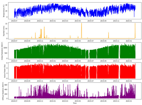
Figure 4. Selection of variables processed over time.

4.1. System Evaluation

The objective of the tests is to verify if there was a significant difference in the treatments applied, and if so, which method was the best. Metrics, such as mean absolute error (MAE), mean square error (MSE), root mean square error (RMSE), and Symmetric Mean Absolute Percentage Error (sMAPE), were used to evaluate the system because it is based on a regression problem. These metrics measure the distance between the predicted value, $\widetilde{Y_i}$, and the actual value, $Y_i$ (real data):

• The Mean Absolute Error (MAE) calculates the average of the errors in the set of predictions. This metric takes into account all individual differences for the same weight. In addition, its value is absolute, so the signs in the errors are eliminated.

  $$MAE=\frac{1}{n}\sum _{j=1}^n|Y_i-{\tilde{Y}}_i|.$$

  (10)
• The Mean Square Error (MSE) measures the average squared error of the actual value of the estimate. This metric was used as the value of the losses in the configuration of the neural network.

  $$MSE=\frac{1}{n}\sum _{i=1}^n{({\tilde{Y}}_i-Y_i)}^2.$$

  (11)
• The Root Mean Square Error (RMSE) is the quadratic scoring rule that measures the average of errors. It calculates the value through the square root of the average squared differences between predictions and actual observations.

  $$RMSE=\sqrt{\frac{1}{n}\sum _{i=1}^n{(Y_i-{\tilde{Y}}_i)}^2}.$$

  (12)
• Symmetric Mean Absolute Percentage Error (sMAPE) is the measure for forecast accuracy based on percentage errors.

  $$sMAPE=\frac{100\%}{n}\sum _{i=1}^n\frac{|Y_i-{\tilde{Y}}_i|}{\left(\right|Y_i|+|{\tilde{Y}}_i\left|\right)/2}.$$

  (13)

The smaller the values of MAE, MSE, RMSE, and sMAPE, the better the performance of a forecasting model. A validation set of 735 instances has been used to test the model. Various configurations were tested by adding a certain number of neurons in various layers of the network. In addition, two test sets were made with different optimization algorithms. The first optimization algorithm that has been used is called Root Mean Square Propagation (RMSprop). The RMSprop algorithm tries to find a smaller oscillation in the gradient slope by choosing a single learning rate for each specific parameter. Table 3 shows the obtained outcome.

Table 3. Root Mean Square Propagation (RMSprop) algorithm test results.

Name	Number of Neurons	MAE	MSE	RMSE
Test 1	Layer1: 6	0.0899	0.0178	0.1334
Test 2	Layer1: 12	0.0904	0.0196	0.1483
Test 3	Layer1: 24	0.0821	0.0165	0.1284
Test 4	Layer1: 48	0.0731	0.0157	0.1254
Test 5	Layer1: 72	0.0744	0.0162	0.1273
Test 6	Layer1: 6 Layer2: 3	0.1160	0.0253	0.1590
Test 7	Layer1: 12 Layer2: 6	0.0751	0.0154	0.1241
Test 8	Layer1: 48 Layer2: 12	0.0730	0.0168	0.1298
Test 9	Layer1: 48 Layer2: 24	0.0749	0.0170	0.1304
Test 10	Layer1: 12 Layer2: 48	0.0745	0.0163	0.1275
Test 11	Layer1: 24 Layer2: 48	0.0740	0.0169	0.1298
Test 12	Layer1: 12 Layer2: 6 Layer3: 3	0.0867	0.0173	0.1315
Test 13	Layer1: 48 Layer2: 12 Layer3: 6	0.0850	0.0186	0.1363

In each of the tests, the number of neurons in the hidden layer of the network was increased to see whether the results improved or not. Up to 72 neurons were tested where it was observed that the obtained result did not improve with the previous test. Then, an attempt had been made to increase the number of layers. The number of neurons was increased in the first layer and decreased in the second, and vice versa. But, starting from the best results of the previous tests, such as 0, 1, and 3, the best configurations obtained were in test 7 and test 8. The number of hidden layers was increased to 3, but there was no improvement in the result. Finally, the most optimal configuration was obtained, where two layers have 12 neurons in the first layer and 6 neurons in the second layer. Test 7 was selected even though it had a higher MAE than test 8, since, in the RMSE, it has a considerably lower value.

A second test has been performed by switching the algorithm using the Adam algorithm. This algorithm is based on algorithms, such as RMSprop, used in the first test, Adadelta, or Momentum. The same configuration of neurons was used as in the previous test in order to make a comparison of the results obtained by both algorithms. The results obtained from these tests are shown in Table 4.

Table 4. Adam algorithm test results.

Name	Number of Neurons	MAE	MSE	RMSE
Test 1	Layer1: 6	0.1035	0.0220	0.1483
Test 2	Layer1: 12	0.0738	0.0155	0.1245
Test 3	Layer1: 24	0.0847	0.0189	0.1374
Test 4	Layer1: 48	0.0704	0.0159	0.1261
Test 5	Layer1: 72	0.0708	0.0159	0.1262
Test 6	Layer1: 6 Layer2: 3	0.2634	0.0875	0.2958
Test 7	Layer1: 12 Layer2: 6	0.0757	0.0154	0.1240
Test 8	Layer1: 48 Layer2: 12	0.0716	0.0157	0.1251
Test 9	Layer1: 48 Layer2: 24	0.0712	0.0162	0.1272
Test 10	Layer1: 12 Layer2: 48	0.0768	0.0165	0.1284
Test 11	Layer1: 24 Layer2: 48	0.0684	0.0141	0.1188
Test 12	Layer1: 12 Layer2: 6 Layer3: 3	0.0762	0.0158	0.1256
Test 13	Layer1: 48 Layer2: 12 Layer3: 6	0.0850	0.0164	0.1280

In order to complete the study, a final analysis is carried out in order to select the best architecture. Tests performed and shown in both Table 3 and Table 4 are filtered out by identifying the two best results and the two worst for each test bank in both algorithms. In this final analysis, the sMAPE metric is incorporated. For the RMSprop algorithm, the worst pair (test 2 and 6) and the best (test 5 and 8) are identified, for which the results are shown in Table 5. The same procedure is carried out by selecting the best results with the Adam algorithm (test 4 and 11) and the worst (test 1 and 6), shown in Table 6. In this second analysis, the sMAPE metric clearly and definitively discriminates the final results.

Table 5. RMSprop algorithm final test results.

Name	Number of Neurons	MAE	MSE	RMSE	sMAPE
Test 2	Layer1: 12	0.0787	0.0174	0.1319	21.56%
Test 5	Layer1: 72	0.0867	0.0205	0.1431	23.06%
Test 6	Layer1: 6 Layer2: 3	0.2634	0.0876	0.2960	30.04%
Test 8	Layer1: 48 Layer2: 12	0.0745	0.0104	0.1281	18.50%

Table 6. Adam algorithm final test results.

Name	Number of Neurons	MAE	MSE	RMSE	sMAPE
Test 1	Layer1: 6	0.0763	0.0172	0.1313	20.94%
Test 4	Layer1: 48	0.0731	0.0174	0.1319	17.09%
Test 6	Layer1: 6 Layer2: 3	0.2634	0.0875	0.2958	29.94%
Test 11	Layer1: 24 Layer2: 48	0.0693	0.0161	0.1267	16.34%

As a result, test 11, shown in Table 6, had the best result even if we compare it with the results of the previous test. The final design of the network was based on two hidden layers; the first one had 24 neurons, and the second one had 48 neurons. In addition, according to the results in Table 6 and in Table 5, better results are achieved when using the Adam algorithm as a gradient optimization algorithm.

A comparison is made between the model proposed in this work and the starting model that has already been introduced and analyzed as a methodological basis in previous sections and described in Reference [14], where a model based on convolutional networks with multiple heads is proposed. Using MAE, RMSE, and sMAPE metrics, Table 7 shows the comparison. The model with which this proposal is compared also uses a neural network as a predictive system to provide the solution, and the same metrics have been used in its evaluation, in order to compare the range of values.

Table 7. Metrics comparison of the proposed model.

Model	MAE	RMSE	sMAPE
The referenced model [14]	0.0917	0.1339	17.94
Proposed Model	0.0693	0.1267	16.34
Improvement %	24.42	5.37	1.6

As a result, Table 7 shows that the proposed model is better than the one in the referenced article. Specifically, it shows that the proposed model has an improvement of 5.37% in RMSE, 24.42% in MAE, and that 1.6% in sMAPE was achieved.

4.2. Model Assessment

Once the final network structure with two hidden layers of 24 and 48 neurons has been selected using Adam’s algorithm, according to the previous section, the evaluation data set can be applied. This way, the results of the proposed case study can be observed. To display the results graphically, graphs, such as the Figure 5, Figure 6, Figure 7 and Figure 8, show the variation of the active power normalized with values between 0 and 1 of the solar panel over the hours. The daily power cycles (24 h) are clearly perceived in Figure 5 and Figure 7 show, reaching the maximum power in the central hours of the day and descending to 0 at night, in the hours when there is no sun.

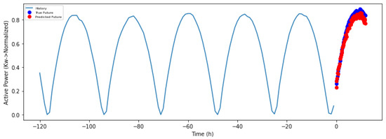
Figure 5. Output power of the solar module in the evaluation window.

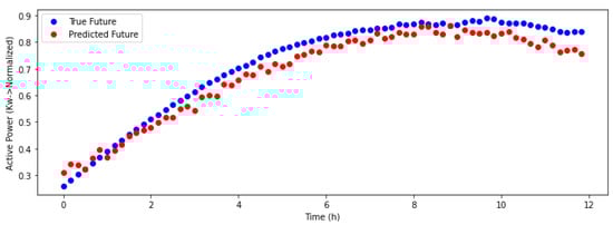
Figure 6. Magnified output power of the solar module in the evaluation window.

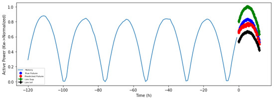
Figure 7. Output power with limit of the solar module in the evaluation window.

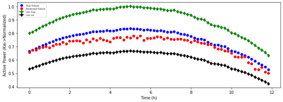
Figure 8. Extended output power with limit of the solar module in the evaluation window.

The neural network has an input time window where parameters, such as global solar panel radiation and diffuse radiation, are entered at each instant of time. This is done by creating a set of data formed by periods that represent these time windows. The neural model processes the input, and, as a result, a forecast is obtained with as many instances as there were neurons in the output.

Figure 5 and Figure 6 show in blue the input window representing the active power of the panel and the resulting output in red. An approach was designed in which a time window was introduced that was composed of a five-day history of measurements and a forecast for the next day. As a result, the output power of the solar panel has been obtained. These results were compared with the real value provided by the data set.

Figure 5 shows the continuous blue line, that represents the normalized power record that the module had in the last 5 days (−120 h). This period of time was the input to the neural network with the normalized global radiation and diffuse radiation values. The output power of the solar panel has been obtained with a 12-h forecast, as can be seen in both Figure 5 and Figure 6, where it is magnified.

The red dots represent the predictions made by the neural network using the input data. The continuous blue line represents the power it has held in the past in the time window, while the blue points are the real values of the solar module in that instant of time.

The confidence margins, which had been detailed in the system description, were applied. These limits are represented graphically to see that the predictions are within the normal values. These results are shown in Figure 7 and Figure 8.

The lower limit is represented by the black line and the upper limit is represented by the green line. It can be seen that the predictions are within the limits calculated as a zone of optimal solar panel performance.

4.3. An Architectural Proposal

To complete the proposal, on the basis of the obtained results, a possible application of the system is proposed within an architecture based on Edge Computing and Big Data ingestion. The objective of the proposed architecture is to allow for the generation and integration of a real-time fault control system for a solar panel infrastructure.

The idea is based on each PV module being associated with an edge node where system operations are performed. The answer would be unique for the associated module and thus save communication costs and latency. Apart from obtaining the data from the board, the node receives the meteorological data from the area in order to make the prediction. The communication data flow would be done through Message Queue Telemetry Transport (MQTT) or similar communications. These communications would be programmed every certain period of time with the cloud to store all the events that take place. The cloud would be in charge of managing all the operations performed by the architecture, apart from recording all plant activity. In addition, a service-based platform would be developed where the entire station could be monitored in real time. This platform would show the predictions that would be made in the nodes. These nodes would in turn manage a series of actuators that control the current flow of the solar panels in case the network has a critical failure. Figure 9 gives an outline of the proposal.

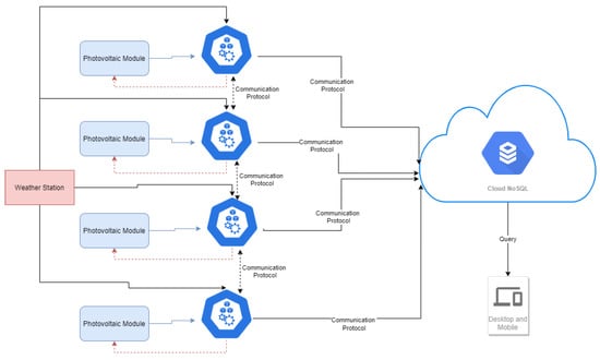
Figure 9. Component scheme of the architectural proposal.

5. Conclusions and Future Work

Throughout the paper, a systematic mapping of predictive maintenance technology has been done, focusing mainly on PV modules for solar energy. A proposal has been defined that is capable of detecting degradation in solar modules.

A neural network has been developed, capable of predicting the output power of solar panels on the basis of weather forecasts. Once obtained, the time window was compared with the real value of the module. By applying some confidence limits, it is possible to determine the possible malfunctioning of the panel. As a result, a predictive model has been obtained in which performance is up to 25.4% better than that of the published proposals.

Additionally, the design of an architecture based on Edge Computing has been proposed, where the developed system would be applied. This architecture would connect the IoT devices and would be able to store large volumes of data in the cloud.

In a future research, the system’s performance will be studied under adverse weather conditions and seasonal changes. The application of different algorithms for the prediction of models based on time series, such as ESNs, will be evaluated, as they have proven to obtain good performance in time series prediction in researches that focused on similar problem presented here. In addition, the proposed architecture will be used for the detection of degradation in solar modules.

References

- Guerrero, M.; Luque Sendra, A.; Lama-Ruiz, J.R. Técnicas de predicción mediante minería de datos en la industria alimentaria bajo el paradigma de Industria 4.0. In V Jornada de Investigación y Postgrado de la Escuela Politécnica Superior de Sevilla; Universidad de Sevilla, Departamento de Ingeniería del Diseño: Sevilla, Spain, 2019; pp. 149–157. ISBN 978-84-120057-2-1. [Google Scholar]
- Lund, H.; Østergaard, P.A.; Connolly, D.; Mathiesen, B.V. Smart energy and smart energy systems. Energy 2017, 137, 556–565. [Google Scholar] [CrossRef]
- Ascencio-Vásquez, J.; Kaaya, I.; Brecl, K.; Weiss, K.A.; Topič, M. Global climate data processing and mapping of degradation mechanisms and degradation rates of PV modules. Energies 2019, 12, 4749. [Google Scholar] [CrossRef]
- Leaman, C. The benefits of solar energy. Renew. Energy Focus 2015, 16, 113–115. [Google Scholar] [CrossRef]
- Pereira, R.I.S.; Jucá, S.C.S.; Carvalho, P.C.M.; Fernández-Ramírez, L.M. Comparative analysis of photovoltaic modules center and edge temperature using iot embedded system. Renew. Energy Power Qual. J. 2019, 17, 198–207. [Google Scholar] [CrossRef]
- Sabry, A.; Hasan, W.; Kadir, M.; Radzi, M.; Shafie, S. Wireless monitoring prototype for photovoltaic parameters. Indones. J. Electr. Eng. Comput. Sci. 2018, 11, 9–17. [Google Scholar] [CrossRef]
- Seyedi, Y.; Karimi, H.; Grijalva, S. Distributed Generation Monitoring for Hierarchical Control Applications in Smart Microgrids. IEEE Trans. Power Syst. 2017, 32, 2305–2314. [Google Scholar] [CrossRef]
- Moreno-Garcia, I.M.; Palacios-Garcia, E.J.; Pallares-Lopez, V.; Santiago, I.; Gonzalez-Redondo, M.J.; Varo-Martinez, M.; Real-Calvo, R.J. Real-Time Monitoring System for a Utility-Scale Photovoltaic Power Plant. Sensors 2016, 16, 770. [Google Scholar] [CrossRef]
- Sun, X.; Chavali, R.V.K.; Alam, M.A. Real-time monitoring and diagnosis of photovoltaic system degradation only using maximum power point-the Suns-Vmp method. Prog. Photovoltaics 2019, 27, 55–66. [Google Scholar] [CrossRef]
- Yasin, Z.M.; Salim, N.A.; Aziz, N.F.A.; Mohamad, H.; Wahab, N.A. Prediction of solar irradiance using grey Wolf optimizer least square support vector machine. Indones. J. Electr. Eng. Comput. Sci. 2019, 17, 10–17. [Google Scholar] [CrossRef]
- Farhadi, M.; Mollayi, N. Application of the least square support vector machine for point-to-point forecasting of the PV power. Int. J. Electr. Comput. Eng. 2019, 9, 2205–2211. [Google Scholar] [CrossRef]
- Rodrigues, S.; Mütter, G.; Ramos, H.G.; Morgado-Dias, F. Machine Learning Photovoltaic String Analyzer. Entropy 2020, 22, 205. [Google Scholar] [CrossRef] [PubMed]
- Wang, F.; Yu, Y.; Zhang, Z.; Li, J.; Zhen, Z.; Li, K. Wavelet decomposition and convolutional LSTM networks based improved deep learning model for solar irradiance forecasting. Appl. Sci. 2018, 8, 1286. [Google Scholar] [CrossRef]
- Alhussein, M.; Haider, S.I.; Aurangzeb, K. Microgrid-level energy management approach based on short-term forecasting of wind speed and solar irradiance. Energies 2019, 12, 1487. [Google Scholar] [CrossRef]
- Dong, N.; Chang, J.-F.; Wu, A.-G.; Gao, Z.-K. A novel convolutional neural network framework based solar irradiance prediction method. Int. J. Electr. Power Energy Syst. 2020, 114, 105411. [Google Scholar] [CrossRef]
- Alsafasfeh, M.; Abdel-Qader, I.; Bazuin, B.; Alsafasfeh, Q.; Su, W. Unsupervised fault detection and analysis for large photovoltaic systems using drones and machine vision. Energies 2018, 11, 2252. [Google Scholar] [CrossRef]
- Fu, L.; Yang, Y.; Yao, X.; Jiao, X.; Zhu, T. A Regional Photovoltaic Output Prediction Method Based on Hierarchical Clustering and the mRMR Criterion. Energies 2019, 12, 3817. [Google Scholar] [CrossRef]
- Dhimish, M.; Mather, P.; Holmes, V. Novel Photovoltaic Hot-Spotting Fault Detection Algorithm. IEEE Trans. Device Mater. Reliab. 2019, 19, 378–386. [Google Scholar] [CrossRef]
- López-Fernández, L.; Lagüela, S.; Fernández, J.; González-Aguilera, D. Automatic evaluation of photovoltaic power stations from high-density RGB-T 3D point clouds. Remote. Sens. 2017, 9, 631. [Google Scholar] [CrossRef]
- Ji, D.; Zhang, C.; Lv, M.; Ma, Y.; Guan, N. Photovoltaic Array Fault Detection by Automatic Reconfiguration. Energies 2017, 10, 699. [Google Scholar] [CrossRef]
- Samara, S.; Natsheh, E. Intelligent Real-Time Photovoltaic Panel Monitoring System Using Artificial Neural Networks. IEEE Access 2019, 7, 50287–50299. [Google Scholar] [CrossRef]
- Maitanova, N.; Telle, J.-S.; Hanke, B.; Grottke, M.; Schmidt, T.; von Maydell, K.; Agert, C. A Machine Learning Approach to Low-Cost Photovoltaic Power Prediction Based on Publicly Available Weather Reports. Energies 2020, 13, 735. [Google Scholar] [CrossRef]
- Liu, S.; Dong, L.; Liao, X.; Cao, X.; Wang, X. Photovoltaic Array Fault Diagnosis Based on Gaussian Kernel Fuzzy C-Means Clustering Algorithm. Sensors 2019, 19, 1520. [Google Scholar] [CrossRef] [PubMed]
- Basterrech, S.; Buriánek, T. Solar irradiance estimation using the echo state network and the flexible neural tree. In Intelligent Data Analysis and Its Applications; Springer: Cham, Switzerland, 2014; Volume I, pp. 475–484. [Google Scholar]
- Sun, X.; Li, T.; Li, Q.; Huang, Y.; Li, Y. Deep belief echo-state network and its application to time series prediction. Knowl. Based Syst. 2017, 130, 17–29. [Google Scholar] [CrossRef]
- Li, Q.; Wu, Z.; Ling, R.; Feng, L.; Liu, K. Multi-reservoir echo state computing for solar irradiance prediction: A fast yet efficient deep learning approach. Appl. Soft Comput. 2020, 95, 106481. [Google Scholar] [CrossRef]
- Duan, Y.; Lv, Y.; Wang, F.-Y. Travel time prediction with LSTM neural network. In Proceedings of the 2016 IEEE 19th International Conference on Intelligent Transportation Systems (ITSC), Rio de Janeiro, Brazil, 1–4 November 2016; pp. 1053–1058. [Google Scholar]
- Ibnu, C.R.M.; Santoso, J.; Surendro, K. Determining the Neural Network Topology: A Review. In Proceedings of the ICSCA ’19: Proceedings of the 2019 8th International Conference on Software and Computer Applications, Penang, Malaysia, 19–21 February 2019; pp. 357–362. [Google Scholar]
- Kingma, D.P.; Ba, J. Adam: A method for stochastic optimization. arXiv 2014, arXiv:1412.6980. [Google Scholar]
- DKASC. Alice Springs 25 Hanwha Solar poly-Si Fixed 2016 | DKA Solar Centre. Available online: http://dkasolarcentre.com.au/download?location=alice-springs (accessed on 23 December 2020).
Publisher’s Note: MDPI stays neutral with regard to jurisdictional claims in published maps and institutional affiliations. |
© 2021 by the authors. Licensee MDPI, Basel, Switzerland. This article is an open access article distributed under the terms and conditions of the Creative Commons Attribution (CC BY) license (http://creativecommons.org/licenses/by/4.0/).