Layer-Wise Network Compression Using Gaussian Mixture Model

Abstract

Due to the large number of parameters and heavy computation, the real-time operation of deep learning in low-performance embedded board is still difficult. Network Pruning is one of effective methods to reduce the number of parameters without additional network structure modification. However, the conventional method prunes redundant parameters up to the same rate for all layers. It may cause a bottleneck problem, which leads to the performance degradation, because the minimum number of optimal parameters is different according to the each layer. We propose a layer adaptive pruning method based on the modeling of weight distribution. We can measure the amount of weights close to zero accurately by applying Gaussian Mixture Model (GMM). Until the target compression rate is reached, the layer selection and pruning are iteratively performed. The layer selection in each iteration considers the timing to reach the target compression rate and the degree of weight pruning. We apply the proposed network compression method for image classification and semantic segmentation to show the effectiveness of the proposed method. In the experiments, the proposed method shows higher compression rate during maintaining the accuracy compared with previous methods.

1. Introduction

Since the growth of Deep Neural Networks (DNNs), significant performance has been achieved in a variety of applications, such as image classification [1,2], object detection [3,4], and semantic segmentation [5,6,7,8]. In general, recent DNNs have been very deep and have tremendous parameters to consider large-scale datasets. This makes DNNs more computationally expensive and memory inefficient. Thus, it is hard to implement in resource limited systems, such as mobile devices or self-driving vehicles.

To address this problem, there are various efforts to reduce the computation and memory size. In image classification, from the conventional convolution network, there are some remarkable ways by proposing the network structure modification or the approximated computation of convolution [9,10,11,12]. Even though they have shown comparable classification accuracy to the state of the art methods with much reduced number of parameters, this approach is not directly adjustable to control the relationship between the number of parameters and the accuracy. In terms of compatibility, it is better to remain the current network structure and make it efficiently. For that purpose, network compression is a popular way to reduce the computation without changing the network structure. Knowledge distillation which transfers the knowledge of big network to small target network [13,14,15,16], bit quantization for saving the memory by quantizing the weight (‘Weight’ in this paper indicates the coefficient of filters using the convolution operation, which is usually trained by the learning process.) of model [17,18,19,20] and network pruning that removes the redundant portion of the network have been studied in the field of network compression.

Network pruning can be categorized into structured and unstructured pruning. Structured pruning removes the channel level of the network [21,22] so that it directly decreases computation complexities of network. Consequently, it brings the speed up; however, it does not reduce memory relatively much. On the other hand, unstructured pruning can save the large memory size without an accuracy drop by removing the weight level of the network [23,24]. Although unstructured pruning needs the special libraries that can skip the computation for pruned weights, it has the advantage that saves the large memory by removing considerable number of weights. Since a mobile phone or a resource-limited embedded system usually has the limited memory, it is more important to compress the amount of weights as much as possible with the minimum accuracy drop that can allow a porting to those systems. In this paper, we try to have this advantage so that we mainly focus on the unstructured pruning method.

Han et al. proposed pruning methods based on weight magnitude, which remove weights lower than the specific threshold [23,25]. Since selecting the threshold affects the performance of the pruned network directly, it is important to determine the appropriate threshold to achieve the target compression rate without performance degradation. Assigning the same threshold through all the layers may prune almost all weights for some layers, which causes failure to train the network or a severe accuracy drop. Another option for removing weights is pruning up to the same rate for all layers. However, it may not be the optimal solution because each layer has a different number of weights and the weight distribution. Because each layer in the deep learning network has the fundamental role that generates a relevant output from an input data, it requires the sufficient number of weights to accommodate the diversity of the target dataset. If most of weights in a specific layer are pruned, that layer cannot be trainable due to incapacity of transferring important information into the next layer. We can regard this problem as one of bottleneck problems, which should be taken into account by network pruning methods.

For example, the first and the last convolution layer of VGG-16 has 1728 and 2.35 M weights, respectively. If we prune all layers with the same rate of 90 percents, the first convolution layer remains only 172 weights that can cause this bottleneck problem, while the last layer remains sufficient weights to be trained as explained in Reference [26]. Figure 1 shows the weight histogram of several convolution layers in VGG-16 network. Figure 1a has a maximum magnitude about 0.4, while Figure 1c has about 0.01. This implies that, when pruning each layer with the same rate, in some layers, relatively large magnitudes are also removed, which leads to the loss of important information. In addition, we can notice that the same threshold cannot be used because some layers are not pruned at all with large thresholds, and some layers are pruned up to the whole weights with small thresholds, as shown in Figure 1.

In this paper, we propose a layer-wise pruning method. To prune each layer adaptively, we should determine the optimal threshold for each layer. In a VGG-16 network, for example, there are 13 convolutional layers and 3 fully connected layers so that we consider 16 threshold values. Our main idea is to use an intuitive idea that the more small magnitude of weights in the layer, the more prune that layer. On this basis, we propose three steps in the pruning procedure. First, the quantity of small magnitude of weights in each layer is estimated using Gaussian Mixture Model (GMM). Second, the target layers to be pruned are selected based on this estimation. The last, the selected layers are pruned with specific compression rate. We repeat these three steps until we achieve the target compression rate. By selecting the target layers with more small weights, the proposed not only can prune relatively small weights effectively but also can alleviate the bottleneck problem.

2. Related Works

Recently, there have been various works on making the DNNs more efficient with respect to the memory and computation. One of common ways is to modify the network structure or to approximate the convolution computation. SqueezeNet [9] reduced the network size using fire module which is composed of a squeeze convolution layer and an expand convolution layer. It achieves better performance by downsampling later. MobileNet [10] decreased the number of parameters using depth-wise and point-wise convolutions. ShuffleNet [11] reduced the computational cost without accuracy drop through a point-wise group convolution and a channel shuffle. EfficientNet [12] simultaneously considered the model’s depth scaling, width scaling, and resolution scaling. Then, it found the optimal rat by experiment. Even though their trained models have much smaller network sizes during maintaining the recognition performance, these methods are not easy to apply another domain directly, for example, in object detection or semantic segmentation.

Instead, there is a way to compress the network. Knowledge distillation compresses the network by transferring the knowledge of the teacher, a big network, to student network, a small network. Hinton et al. [27] showed that a small network imitates the soft max of a large network so that knowledge can be transferred. For better generalization and faster execution, Fitnets suggested that not only outputs but also intermediate layers can be resembled to a big network [13]. Due to the characteristic of sequential layer in DNNs, Yim et al. [14] transferred the distilled knowledge considering the flow between layers. However, it is not easy to transfer the knowledge if a gap between teacher and student is large. Mirzadeh et al. [15] alleviated this gap by introducing a teacher assistant so that they achieved better performance. Because the teacher’s performance should be guaranteed for this teacher-student distillation network, Zhang et al. [16] suggested self knowledge distillation without the teacher network. For more detailed surveys of different knowledge distillation methods, we refer the readers to Reference [28].

Another way to reduce the network resource is a network pruning which removes less meaningful connection from the trained network. Network pruning can be classified into structured and unstructured pruning. Structured pruning removes less important or redundant filters so that it reduces each layer’s channel size. Unstructured pruning removes less meaningful or redundant weights during remaining the original structure. Both methods can be directly applied to other existing networks, such as a classification network [1,10,29] or semantic segmentation network [6,30].

To prune redundant channels or filters, structured pruning has been usually approached as an optimization problem. ThiNet (Thin Net) [31] used statistic information computed from its next layer for the filter level pruning. NISP (Neuron Importance Score Propagation), in Reference [32], measures the importance of the final response layer and formulates network pruning as a binary integer optimization problem. Wen et al. [33] compressed the network by applying group Lasso regularization in training. Li et al. [21] selected unimportant filters via L1-norm. Then, they adopted a one-shot pruning and retraining strategy. As adopting the regularization at batch normalization, Liu et al. [34] made scaling factors in batch normalization to zero using L1 regularization that can remove unnecessary channels. FPGM [22] pruned the filter that can be replaced other filters via a Geometry median. Although structured pruning methods simultaneously reduce the computation and the number of weights by removing filters, they cannot prune redundant weights at all. There may be unremoved filters because some weights have important information by applying the filter.

Unstructured pruning aims to remove the weight as much as possible by minimizing an accuracy drop. Optimal Brain Damage (OBD) [35] was proposed to remove the unimportant weights using second-derivative information. Han et al. [23] pruned the network based on weights magnitude and deep compression [25] applied quantization and Hoffman coding for further network efficiency. Net-trim [36] learned sparse parameters for each layer by minimizing reconstructed error. However, this method failed to achieve high compression rate due to difficulty in optimization induced from an $l_0$-norm or an $l_1$ norm regularization term. Dong et al. [37] overcame this problem based on second order derivatives of a layer-wise error function. Tartaglione et al. [38] proposed the method that quantifies the output sensitivity to the parameters and lowers the absolute value of parameters gradually. AutoPrune [24] automatically eliminated network redundancy with recoverability, relieving the complicated prior knowledge required to design thresholding functions.

3. The Proposed Method

The method for pruning the weight in the DNN is based on the magnitude of weights. Simply, we can remove weights that are smaller than the specific threshold. Since the weight distribution may be different according to the layer as in Figure 1, the weights can be over- or under-pruned using a single threshold. Another way for weight pruning is reducing the pre-defined percentage of weights for each layer [23,25]. Even though these methods with the same rate for each layer guarantee the number of remaining weights to some extent, they can suffer from the bottleneck problem due to extremely small number of weights for the specific layer.

To solve the limitation of previous methods, we propose a layer-wise pruning method that removes more weights for the layer including smaller weights close to zero. First, we fit Gaussian Mixture Model (GMM) to the distribution of weights for each layer. Then, layers are selected according to the probability that weights are zero. Finally, weights are pruned with the specific rate in the selected layers.

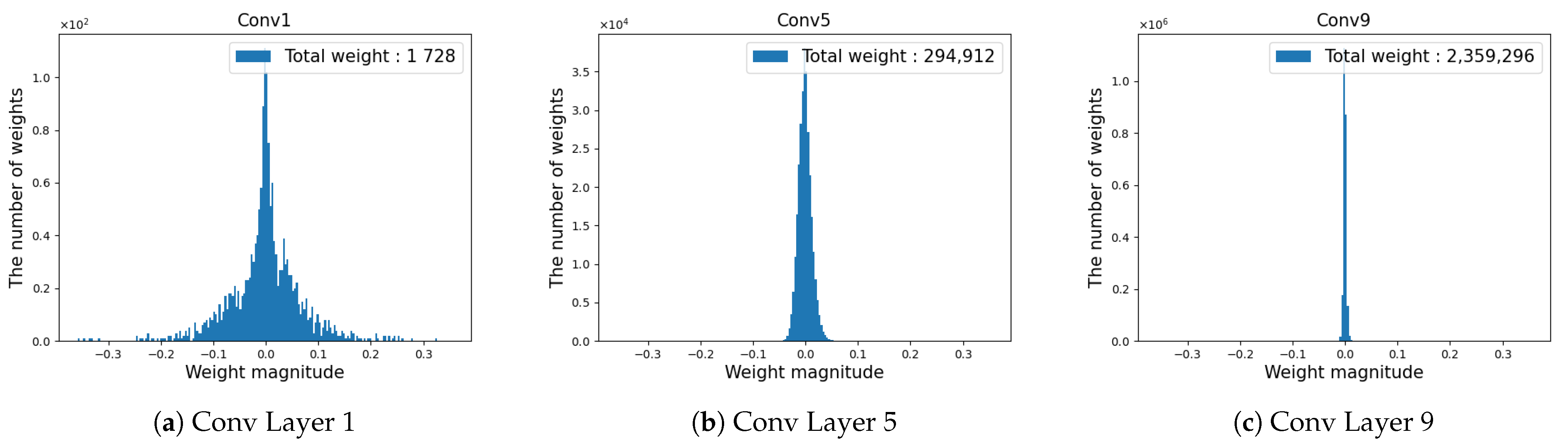
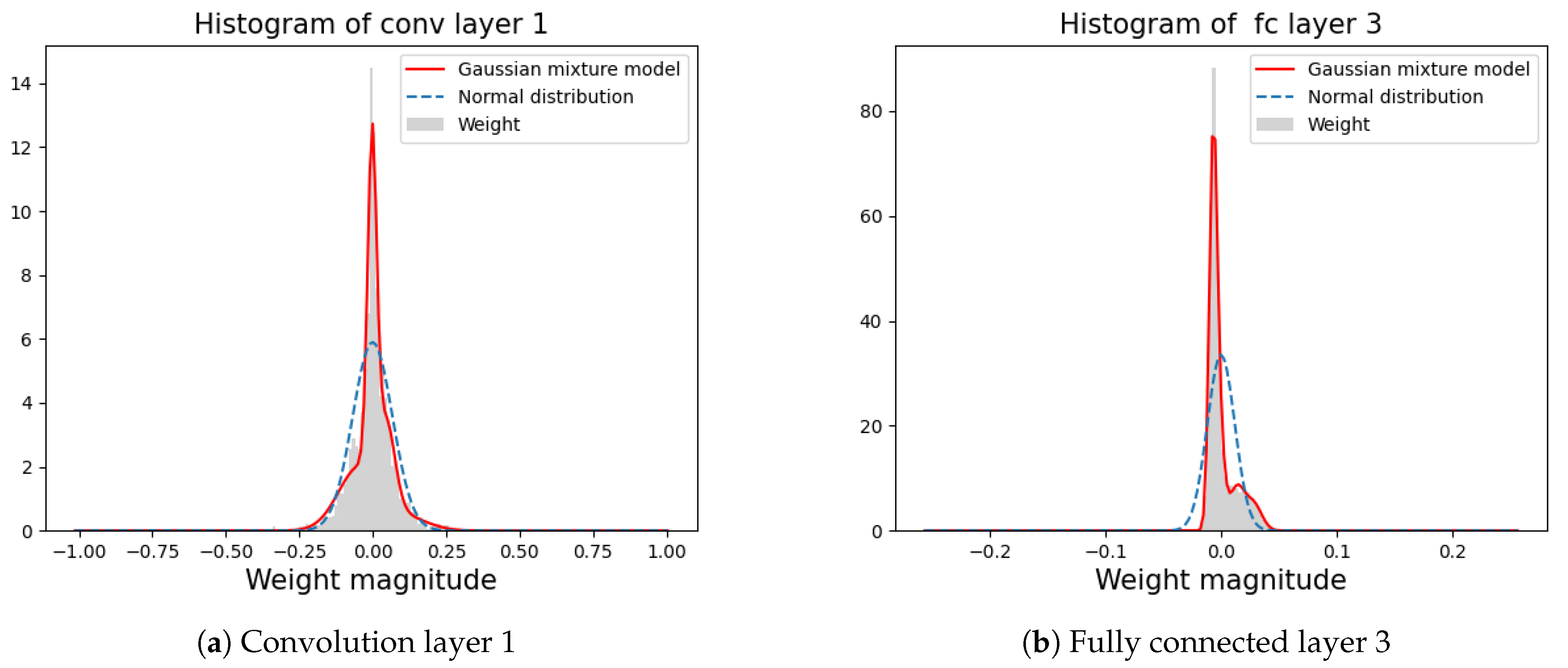
3.1. Estimating the Weight Distribution Using the GMM

For layer-wise pruning, the evaluation for each layer should be done by counting the number of weights close to zero. Intuitively, after constructing a histogram of weights, the value corresponding to zero can be counted as the number of zeros in the layer. However, as shown in Figure 1, a bin width in the histogram is not easy to determine due to the scale variation in each layer. Instead of using the histogram, the Gaussian Mixture Model (GMM) is used to fit the distribution of weights in the layer. To initialize parameters of Gaussian distributions, a K-means clustering algorithm is used to minimize the objective function as:

$$\underset{\mathbb{S}}{argmax}\sum _{i=1}^K\sum _{w\in S_i}\parallel w-{\mu }_i{\parallel }^2,$$

(1)

where $\mathbb{S}=\{S_1,S_2,...,S_K\}$ is a set of K clusters that have a mean ${\mu }_i$, respectively. After random initialization, associating all weights and computing centroids for each cluster are alternately repeated until convergence.

A GMM model that represents a distribution of weights in a layer can be written as:

$$f\left(w\right)=\sum _{i=1}^K{\pi }_i\mathcal{N}\left(w\right|{\mu }_i,{\sigma }_i),$$

(2)

where ${\pi }_i$ is the mixing coefficients, where:

$$\sum _{i=1}^K{\pi }_i=1and{\pi }_i\ge 0,\forall i.$$

(3)

$\mathcal{N}(·|{\mu }_i,{\sigma }_i)$ is an i-th Gaussian distribution with mean ${\mu }_i$ and standard deviation ${\sigma }_i$. To estimate more accuracy parameters in each Gaussian distribution from the initial values, the Expectation and Maximization (EM) algorithm is applied to find maximum likelihood solutions. In E-step, given the current estimate of the parameters, the conditional probability of a latent variable z which represents the assignment to one of Gaussians can be computed by:

$$p(z=i|w)=p\left(z\right|w)=\frac{{\pi }_i\mathcal{N}\left(w\right|{\mu }_i,{\sigma }_i)}{{\sum }_{j=1}^K{\pi }_j\mathcal{N}\left(w\right|{\mu }_j,{\sigma }_j)}.$$

(4)

In M-step, the parameters of Gaussians are re-estimated given the current assignments as:

$${\mu }_i=\frac{1}{N_i}\sum _{n=1}^{N}p\left(z^{\left(n\right)}\right|w)w^{\left(n\right)},$$

(5)

$${\sigma }_i=\frac{1}{N_i}\sum _{n=1}^{N}p\left(z^{\left(n\right)}\right|w)(w^{\left(n\right)}-{\mu }_i){(w^{\left(n\right)}-{\mu }_i)}^T,$$

(6)

$${\pi }_i=\frac{N_i}{N}where{N}_i=\sum _{n=1}^{N}p\left(z^{\left(n\right)}\right|w),$$

(7)

where $w^{\left(n\right)}$ and $z^{\left(n\right)}$ indicate n-th weight and its assignment, respectively. N is the total number of weights.

Figure 2 shows the modeling results for convolution layer 1 and fully connected layer using the proposed GMM model and the conventional normal distribution. It is shown that the distributions of weights cannot be modeled by a single Gaussian distribution due to their non-symmetric and one-sided properties. The weight distribution is well fitted by the proposed GMM model based on the initialization and iterative parameter estimation using the K-means clustering and EM algorithm, respectively. From this accurate fitting results of weight distributions, we can estimate the probability of weights on the value of zero.

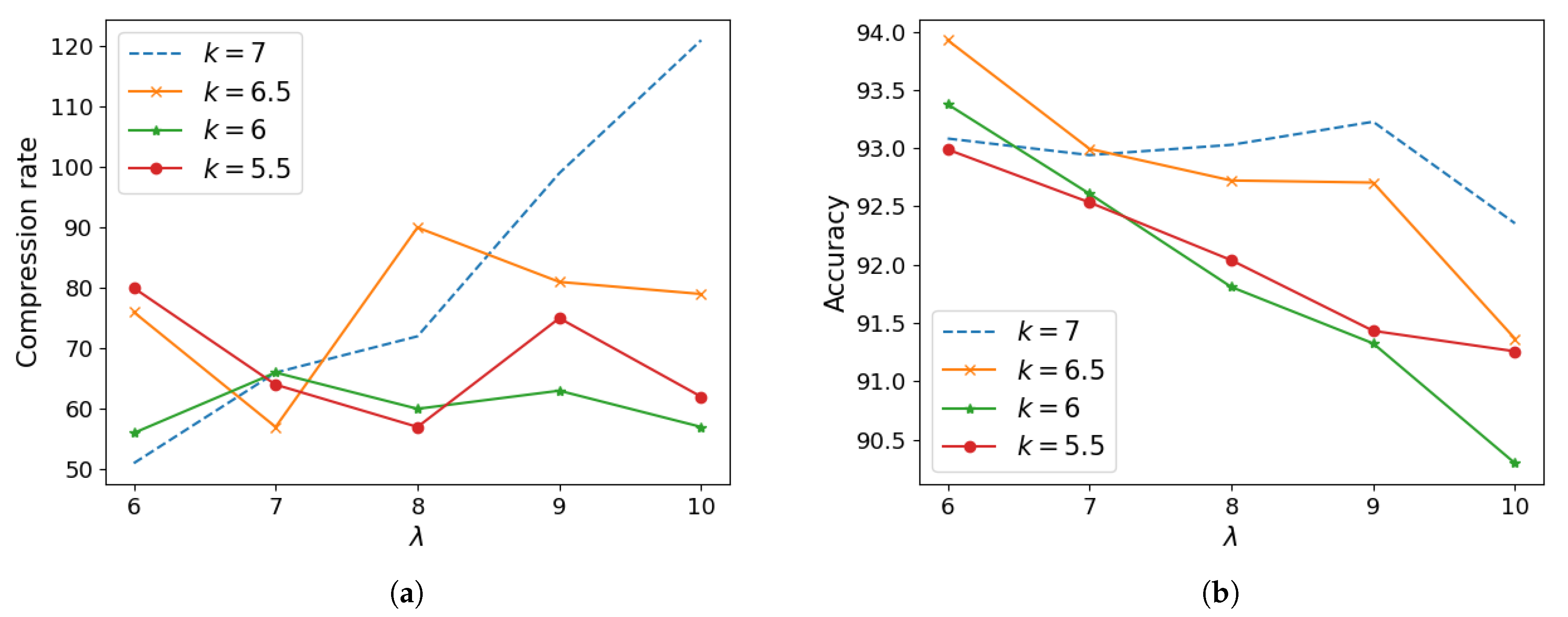
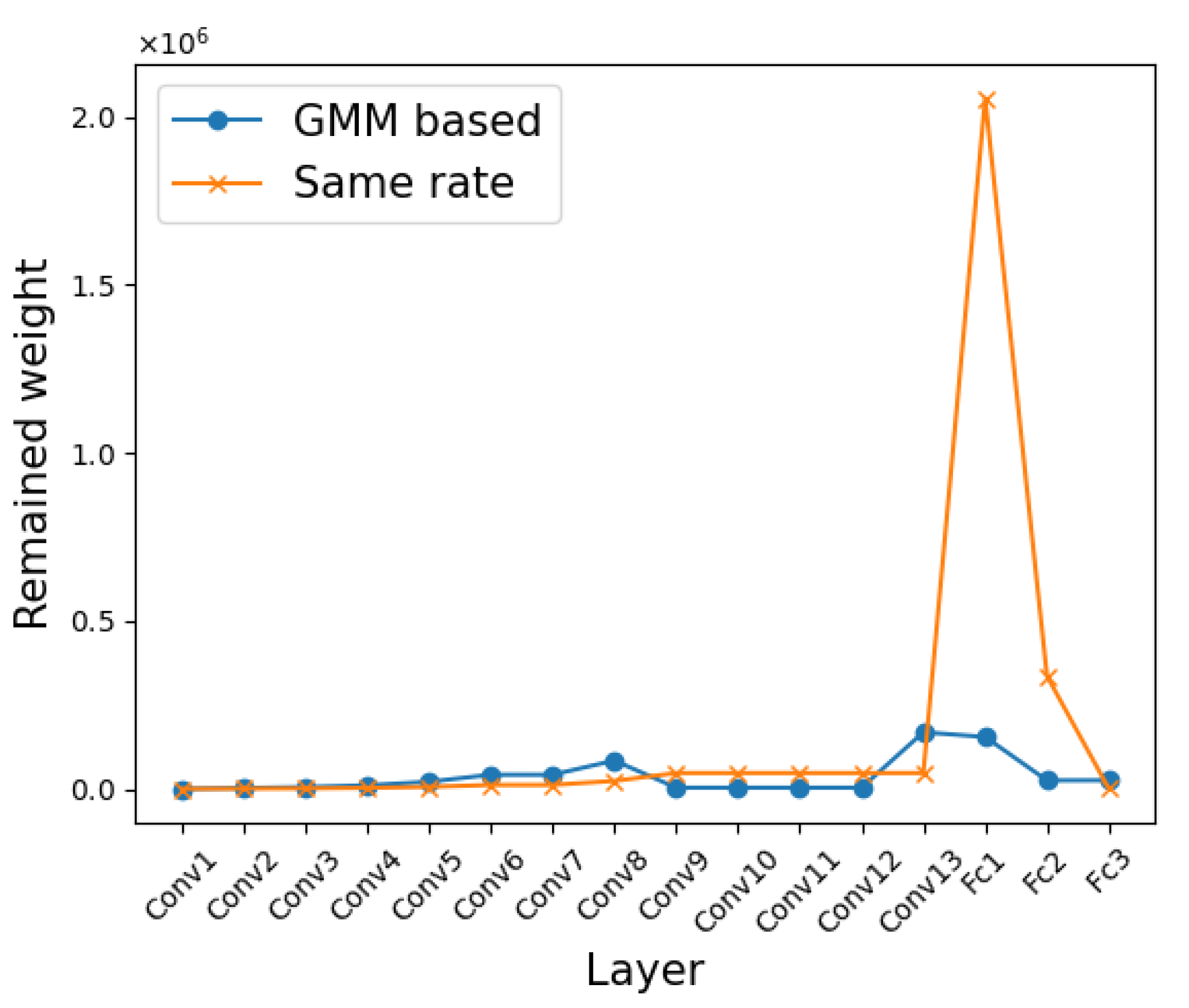
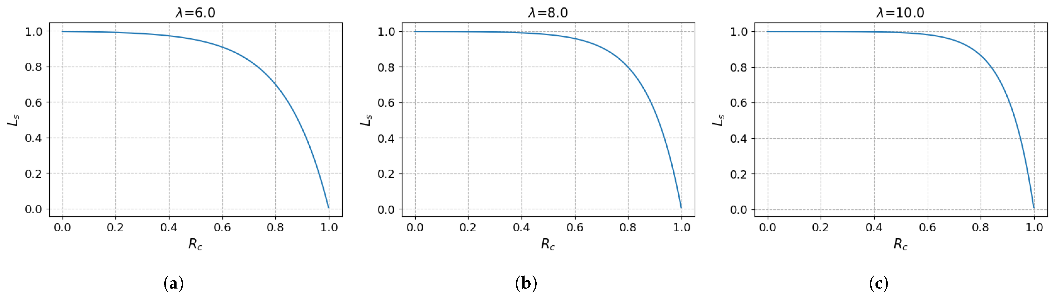
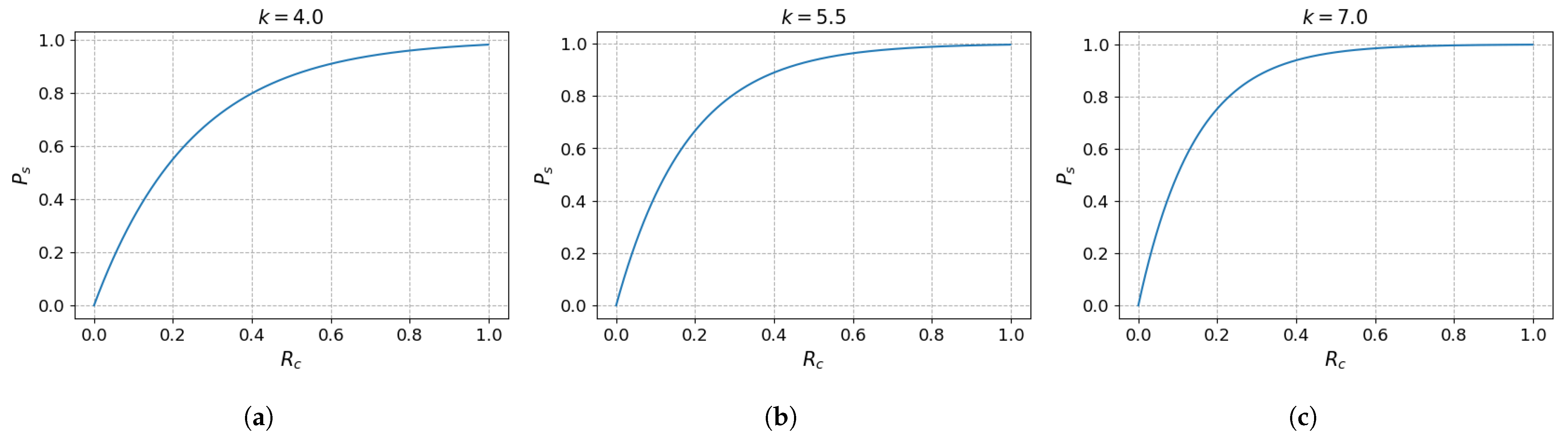
3.2. Layer Selection According to Redundancy

Instead of pruning all the layers in each step, the layers to be pruned in this step are selected according to the probability of zero weights because the layer that the number of weights close to zero is larger can have more redundant weights. However, the determination how many layers are selected in a single step is the corresponding problem. If the number of selected layers is too small, it will take a long time to achieve the target compression rate or fail to reach it. On the other hand, if the number of selected layers is too large, it can achieve the target compression rate quickly, but our layer-wise pruning scheme according to redundancy become less effective. To solve this issue, we determine the number of selected layers as:

$$L_s=1-\frac{e^{\lambda \times R_c}}{e^{\lambda }}.$$

(8)

$L_s$ is the rate of layers to be selected, which is determined by current compression rate, $R_c$. $R_c$ is a value between 0 and 1. In the earlier step, the large number of layers are selected. This ensures that it prunes all the layers in the early steps to achieve the target compression rate efficiently. As the steps go by, the number of selected layers decreases gradually to remove weights only at the relatively more redundant layers. $\lambda$ determines the steepness of decreases, as shown in Figure 3. It controls the trade-off between the training time to reach the target compression rate and the rapid consideration of more redundant layers.

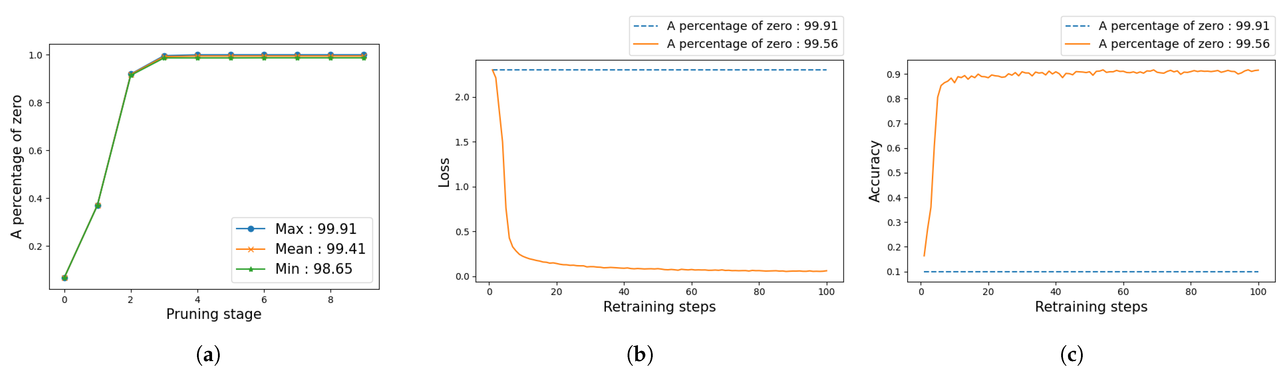
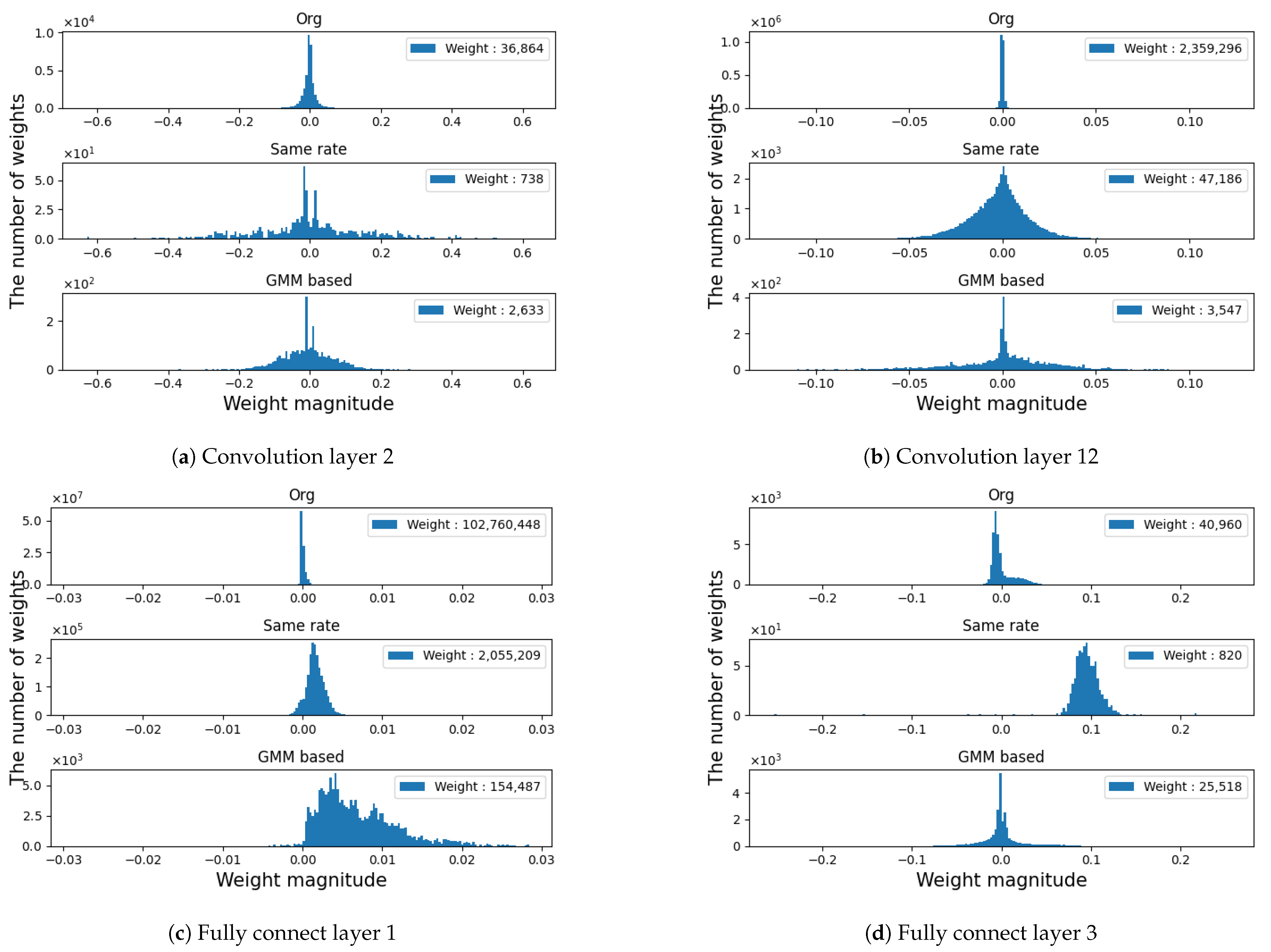
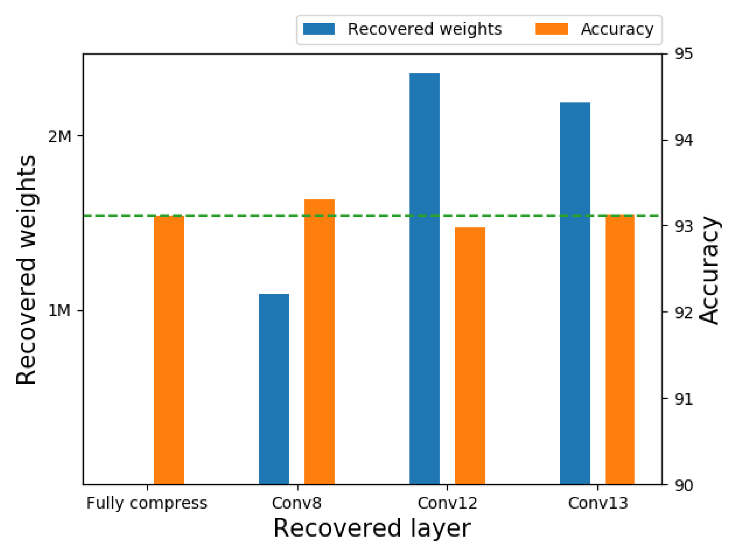
3.3. Pruning of Selected Layers

The last procedure of our method is pruning selected layers. We chose the large number of layers to be pruned in earlier steps to reach the target compression rate rapidly. Because the distribution in each layer is different, applying a large compression rate at this step would remove important weights at once, which results in performance degradation. To prevent this problem, we apply a small compression rate at earlier step and gradually increase the compression rate to reach the target compression rate as:

$$P_s=1-e^{-k\times R_c}.$$

(9)

$P_s$ is a pruning rate in the current step and k is the parameter that control the steepness to reach the target compression rate. $P_s$ is also determined by the current compression rate $R_c$. When the network is extremely compressed, the pruning rate in some layers would be up to 100 percent, which means all weights are removed. However, applying Equation (9) in each step, we can prevent this problem.

In Figure 4, the graph of $P_s$ according to $R_c$ and k. As the current compression rate increases, the value of pruning rates increases gradually. By changing the value of K, the momentum close to the higher pruning rate can be adjusted. The control parameters, $\lambda$ and k, should be considered simultaneously for the final compression rate and classification accuracy.

4. Experiments

In this section, we apply our layer-wise pruning algorithm not only to image classification, which is usually utilized by other network compression methods, but also to semantic segmentation, which shows that our method can be used in other deep learning networks.

4.1. Image Classification

We apply our method to a VGG network [1], which is one of representative networks in image classification. The VGG network is the standard DNN that consists of convolution layer and FC (fully connected) layer. In particular, VGG-16 is a very heavy network consisting of 13 convolution layers and 2 FC layers, and it has 134M of parameters. Many researches have attempted to compress this large-size network because it is not easy to operate in the resource limited devices.

We use the CIFAR10 dataset to evaluate the classification performance. For implementation, we use the pytorch library (1.5.0 verison). The reference model trained with a SGD (Stochastic Gradient Descent) optimizer with decaying learning rate starting from $0.01$ and achieved 7.03% error. The target compression rate is over 98%, which is the same as 50 times (×50) by the pruning process. For the comparison, we refer the performance of other methods in AutoPrune [24]. In

Table 1. Comparison of different unstructured pruning method applying to VGG -16.

Methods	CR	Error Rate
Zhuang et al. [39]	×15.58	6.42% $\stackrel{}{\to }$ 6.69%
Zhu et al. [40]	×8.5	6.01% $\stackrel{}{\to }$ 5.43%
Sparse VD [41]	×65	7.55% $\stackrel{}{\to }$ 7.55%
AutoPrune [24]	×75	7.60% $\stackrel{}{\to }$ 7.82%
GMM-Based-Layerwise [Ours]	×225	7.03% $\stackrel{}{\to }$ 6.89%

, when we use the same rate to compress VGG-16 to the ×50, an error rate increased from 7.03% to 10.99%. This accuracy drop is rather severe to employ it practically. Because the methods in Zhuang et al. [39] and Zhu et al. [40] can be categorized as channel pruning, their performance in terms of compression rate is comparably lower than other methods. However, they have another advantage of reducing computational cost effectively due to direct removal of channels. Sparse VD to the ×65 with no accuracy drop. In case of AutoPrune [24], they compressed VGG-16 up to ×75 with little accuracy drop, 0.22%. Applying the proposed layer-wise method to compress VGG-16, the network is shrunk up to ×225, and the error rate decreases to 6.89%. The proposed method can generate the highly efficient network where remaining weights are less than 1% of total weights with accuracy improvement from the baseline, as in Table 1. It validates that the proposed pruning strategy based on GMM-based weight modeling is effective.

The remaining weight and compression rate for each layer is shown in

Table 2. Remaining weights and compression rate for each layer in VGG-16.

Layer	Weight	Remaining Weight	Rate of Remainder
Conv 1	1728	124	7.18%
Conv 2	37 K	2.6 K	7.14%
Conv 3	74 K	5.2 K	7.14%
Conv 4	147 K	11 K	7.14%
Conv 5	294 K	21 K	7.14%
Conv 6	590 K	42 K	7.14%
Conv 7	590 K	42 K	7.14%
Conv 8	1.18 M	84 K	7.14%
Conv 9	2.36 M	3.5 K	0.15%
Conv 10	2.36 M	3.5 K	0.15%
Conv 11	2.36 M	3.5 K	0.15%
Conv 12	2.36 M	3.5 K	0.15%
Conv 13	2.36 M	169 K	7.14%
FC 1	102.76 M	154 K	0.15%
FC 2	16.78 M	25 K	0.15%
FC 3	41 K	26 K	62.3%
Total	134 M	596 K	0.44%

. In VGG-16, from Conv 1 to Conv 8 are compressed at a relatively small rate. This means that there are relatively larger magnitude in the front side of the network with less redundancy. The layers in the back side of convolution layers from Conv 9 to Conv 12 and the FC layers 1 and 2 are massively pruned due to the large portion of small weights. Even though the huge number of parameters are pruned, it does not have a significant impact on performance. Interestingly, the compression rate of the final FC layer is comparably low. It means that the final layer includes important information that has weights of large magnitude.

In Table 2, we can notice that VGG-16 has highly weight redundancy with a meaningful value of only 0.6 M out of 134 M. Because the rate of remainder is different according to layers, we can assume that the rate of remainder for a specific layer indicates the importance of that layer. We select Conv 8 as a more important layer and Conv 12, 13 as less important layers according to their rates of remainders in Table 2. As in Figure 5, by recovering Conv 8, which means not compressing Conv 8, we can achieve a more accurate result than the fully compressed model in Table 2 with 1 M more weights. However, by recovering Conv 12 or 13, the accuracy is similar or even worse than the fully compressed model even though they have 2 M more weights. From this experiment, we can notice that, if the rate of remainder is higher for a layer, i.e., if the layer is less redundant after applying the proposed layer-wise weight pruning method, we can regard the layer as a more important layer.

Recently, efficient networks have been introduced by modifying the network structure or approximating the convolution computation, like MobileNet [10]. MobileNet is one of good options when we develop applications running in a mobile phone or an embedded board. However, according to target platform, we may need more reduced network due to the limitation of memory or processing time. As in

Table 3. The results by applying our method to MobileNetV2 and GoogleNet (CIFAR10 dataset).

Network	Method	Accuracy	CR	No. of Weights
MobileNet [42]	Original	94.59	-	2.2 M
	pruned by our method	94.11	×6.01	0.36 M
GoogleNet [29]	Original	92.63	-	6.14 M
	pruned by our method	91.96	×10.78	0.57 M

, the proposed method can reduce the number of weights up to less than 20% of original MobileNet network, while an accuracy drop is less than 0.5%. Because the filter size of VGG-16 and MobileNet is $3\times 3$, we applied our method to GoogleNet [29], which has $5\times 5$ filters. Our method compressed GoogleNet less than 10% from the original network, while an accuracy drop is less than 1%, as shown in Table 3. From these experiments, we can show that the proposed method can be applied to various networks, regardless of network efficiency and mask size.

To show the limitation of the amount of network size reduction, we have tried to compress the network as much as possible. As in Figure 6a, a percentage of zeros is from 98.65% to 99.91% when we tried 5 times. Interestingly, the loss is totally not reduced as a retraining step is processed when a percentage of zeros is the maximum value of 99.91% in Figure 6b. Consequently, the accuracy is not increased for the case in Figure 6c. When the network is severely reduced so that a specific layer with significantly small remaining weights cannot transfer relevant information into the next layer, the training cannot be proceeded due to the bottleneck problem explained in Section 1. When a percentage of zeros is not the maximum value, we can see that the loss becomes reduced, and the accuracy is increased, as shown in Figure 6b,c. There is the limitation of network size reduction, which the network cannot be trainable due to the bottleneck problem. We should consider that the compressed network does not reach to this maximum value during the process of network compression.

In Equations (8) and (9), there are control parameters, $\lambda$ and k, which can affect the performance of the proposed pruning method. Accordingly, we show the compression rate and accuracy according to varying $\lambda$ and k values in Figure 7. We tested k from 5.5 to 7 with 0.5 interval, and $\lambda$ from 6 to 10 with 1 interval. Each value of compression rate and accuracy is obtained by averaging of performing 5 times. In case of small k, there is no further compression through $\lambda$ is increasing. On the other hand, when k is sufficiently large, the network is more compressed according to the increase of $\lambda$, as in Figure 7a. In addition, in Figure 7b, accuracy decreases relatively slowly at $k=7$. Therefore, the compression rate and accuracy have the trade-off relationship when we select sufficiently large k values. We select $k=7$ and $\lambda =9$ for all of our experiments.

As mentioned earlier, the performance could be degraded when the specific layers are pruned severely due to the bottleneck problem. Figure 8 shows the weight distribution after the training in the original network, the pruned network using the same rate, and the pruned network based on GMM, respectively. In the layer of small number of weights, as shown in Figure 8a,d, the distribution of weights has different profiles from the original or GMM-based network due to the same rate pruning applied to initially small number of weights. Furthermore, in FC layer 3, most weights around the zero are pruned. Contrarily, in the layer of large number of weights in Figure 8b,c, the great number of weights close to zero are remaining redundantly in the same rate pruning method compared with the GMM-based pruning method. From this layer-level analysis of weight distributions, the proposed GMM-based pruning method not only preserves the sufficient number of weights in the small-sized layers to escape from the bottleneck problem but also reduces the redundant number of weights to compress the network more effectively.

In Figure 9, we show that the number of remaining weights for each layer in the same rate pruning and GMM-based pruning methods, respectively. Compared with the same rate pruning, the proposed layer-wise pruning has more weights from conv5 to conv9 layers but less weights from conv9 to conv12. Because the FC1 and FC2 layers are pruned considerably, we can notice that these layers have very high redundancy compared with other layers.

4.2. Semantic Segmentation

We apply the proposed method to another deep learning network to show the effectiveness of our method. Semantic segmentation is widely used in variety of applications, such as self-driving. FCN (fully connected network) [5] proposed the 1 × 1 convolution to enable segmentation through DNNs. However, FCN is hard to run in real-time due to high computational cost. To reduce the computational cost, SegNet [30] was proposed, which reduces the trainable parameters to execute in real time on the device with the strong computing power, such as Nvidia TitanX GPU. But, they still have the 29 M parameter, which could not run in real-time on the resource limited device.

We pre-trained a SegNet model using NYUv2 Dataset with an SGD optimizer with decaying learning rate starting from $0.01$, which is implemented using the pytorch library (1.5.0 verison). We attempt to compress the model to the 98% over as in Section 4.1. We compute the accuracy (pixel-wise accuracy $=\frac{TN+TP}{TN+TP+FN+FP}$) and mIoU (mean intersection over union $=\frac{1}{N_{class}}{\sum }_{N_{class}}\frac{target\cap prediction}{target\cup prediction}$) to show our method’s performance. In

Table 4. Comparison of unstructured pruning method applying to SegNet.

Methods	CR	Remaining Weight	Accuracy	mIoU
SegNet [30]	-	29 M	57.71	20.50
Same Rate [23]	×50	0.58 M	53.64	16.90
GMM-Based-Layerwise (Ours)	×64	0.44 M	55.27	17.90

, accuracy and mIoU of the reference model are 57.71 and 20.50, respectively. When compressing this model to ×50 using the same rate pruning method [23], the accuracy and mIoU drop to 53.64 and 16.90, respectively. Our compression method reduces up to compression rate of ×64, while the accuracy and mIoU are 55.27 and 17.90, respectively. For semantic segmentation network, the proposed method shows less accuracy drops, as well as higher compression rate, compared with the conventional pruning method [23]. From the result, only 0.44 M out of 29 M parameters can be used with moderate accuracy drops. Because semantic segmentation should compute pixel-level classification labels, it has more accuracy drops than image-level classification. It means that the weights in the semantic segmentation have less redundancy.

In

Table 5. Remaining weights and compression rate for each layer in SegNet.

Layer	Weight	Remaining Weight	Rate of Remainder
Encoder 1	1728	1.1 K	66.44%
Encoder 2	37 K	4.2 K	11.27%
Encoder 3	74 K	8.3 K	11.27%
Encoder 4	147 K	16.6 K	11.27%
Encoder 5	295 K	33.3 K	11.27%
Encoder 6	590 K	1.8 K	0.31%
Encoder 7	590 K	1.8 K	0.31%
Encoder 8	1.18 M	3.7 K	0.31%
Encoder 9	2.36 M	7.4 K	0.31%
Encoder 10	2.36 M	7.4 K	0.31%
Encoder 11	2.36 M	7.4 K	0.31%
Encoder 12	2.36 M	7.4 K	0.31%
Encoder 13	2.36 M	7.4 K	0.31%
Decoder 1	2.36 M	266.1 K	11.27%
Decoder 2	2.36 M	7.4 K	0.31%
Decoder 3	2.36 M	7.4 K	0.31%
Decoder 4	2.36 M	7.4 K	0.31%
Decoder 5	2.36 M	7.4 K	0.31%
Decoder 6	1.18 M	3.7 K	0.31%
Decoder 7	590 K	1.8 K	0.31%
Decoder 8	590 K	1.8 K	0.31%
Decoder 9	295 K	0.9 K	0.31%
Decoder 10	147 K	16.6 K	11.27%
Decoder 11	74 K	8.3 K	11.27%
Decoder 12	37 K	4.2 K	11.27%
Decoder 13	7.5 K	0.8 K	11.28%
Total	29 M	0.44 M	1.5%

, the remaining weights and compression rates are shown for each layer when applying the proposed method. The initial layers in the encoder network are more relevant than the last layers. Contrarily, the initial layers in the decoder network are more redundant than the last layers except for the connecting layer between encoder and decoder networks. This information can be helpful to design an efficient network for semantic segmentation.

To show the effectiveness of the propose pruning method, we apply our method to recent efficient semantic segmentation network, ENet [6]. Although ENet was designed to achieve more than 10 fps on the low-resource device, Nvidia TX1, the network compression enables to apply it to the embedded board with lower specification or without GPU. As shown in

Table 6. Apply our method on ENet with a CamVid dataset.

Methods	mIoU	CR	Remaining Weight
Original ENet [6]	52.85	-	0.34 M
Pruning 50%	53.04	×2.35	0.15 M
Pruning 70%	51.52	×3.51	0.10 M

, the proposed method not only reduces the half of weights from the original ENet [6] but also improves the accuracy of mIoU slightly. This accuracy improvement might be caused that the pruning method has a similar effect of the dropout method to generalize the network. If we pruned more than half, for example, $70\%$, mIoU is dropped more than $1\%$. This tendency is due to generalization-stability trade-off [43] and shows that the redundancy of ENet is not severer than SegNet. The proposed method can be applied semantic segmentation networks, SegNet and ENet, to reduce the number of weights during maintaining the accuracy.

5. Conclusions

We proposed layer-wise pruning method based on the fact that the layer which has more small-valued weights are pruned with higher compression rate. The pruning method has three steps. First, we need to evaluate the redundancy of each layer by estimating the probability of weights on zero. We applied the Gaussian Mixture Model (GMM) to fit the distribution of weights accurately. The second step is selecting the number of layers to be pruned. The selected layers started from all of layers for the fast convergence to target compression rate in early stage and gradually reduced for careful selection in later stage. Finally, the pruning is done with applying lower compression rate for almost all of layers, as well as higher compression rate for carefully selected layers. We applied the proposed method to the image classification and showed better performance than the existing methods in terms of compression rate and classification accuracy. We achieved ×255 compression rate, even with slight improvement of accuracy. By applying to semantic segmentation, our method showed better compression and less accuracy drop compared with the conventional method with the same rate pruning for all layers. By various experiments, we validated that the layer-wise pruning can reduce the number of redundant weights efficiently with the limited accuracy drop.

References

1. Simonyan, K.; Zisserman, A. Very Deep Convolutional Networks for Large-Scale Image Recognition. In Proceedings of the International Conference on Learning Representations, San Diego, CA, USA, 7–9 May 2015. [Google Scholar]
2. He, K.; Zhang, X.; Ren, S.; Sun, J. Deep residual learning for image recognition. In Proceedings of the IEEE Conference on Computer Vision and Pattern Recognition, Las Vegas, NV, USA, 27–30 June 2016; pp. 770–778. [Google Scholar]
3. Girshick, R.; Donahue, J.; Darrell, T.; Malik, J. Rich feature hierarchies for accurate object detection and semantic segmentation. In Proceedings of the IEEE Conference on Computer Vision and Pattern Recognition, Columbus, OH, USA, 24–27 June 2014; pp. 580–587. [Google Scholar]
4. Girshick, R. Fast R-CNN. In Proceedings of the IEEE International Conference on Computer Vision, Santiago, Chile, 11–18 December 2015; pp. 1440–1448. [Google Scholar]
5. Long, J.; Shelhamer, E.; Darrell, T. Fully convolutional networks for semantic segmentation. In Proceedings of the IEEE Conference on Computer Vision and Pattern Recognition, Boston, MA, USA, 8–10 June 2015; pp. 3431–3440. [Google Scholar]
6. Paszke, A.; Chaurasia, A.; Kim, S.; Culurciello, E. Enet: A deep neural network architecture for real-time semantic segmentation. arXiv 2016, arXiv:1606.02147. [Google Scholar]
7. Hu, X.; Yang, K.; Fei, L.; Wang, K. ACNET: Attention Based Network to Exploit Complementary Features for RGBD Semantic Segmentation. In Proceedings of the 2019 IEEE International Conference on Image Processing (ICIP), Taipei, Taiwan, 22–25 September 2019; pp. 1440–1444. [Google Scholar]
8. Yang, K.; Hu, X.; Fang, Y.; Wang, K.; Stiefelhagen, R. Omnisupervised Omnidirectional Semantic Segmentation. IEEE Trans. Intell. Transp. Syst. 2020, 1–16. [Google Scholar] [CrossRef]
9. Iandola, F.N.; Han, S.; Moskewicz, M.W.; Ashraf, K.; Dally, W.J.; Keutzer, K. SqueezeNet: AlexNet-level accuracy with 50x fewer parameters and <0.5 MB model size. arXiv 2016, arXiv:1602.07360. [Google Scholar]
10. Howard, A.G.; Zhu, M.; Chen, B.; Kalenichenko, D.; Wang, W.; Weyand, T.; Andreetto, M.; Adam, H. Mobilenets: Efficient convolutional neural networks for mobile vision applications. arXiv 2017, arXiv:1704.04861. [Google Scholar]
11. Zhang, X.; Zhou, X.; Lin, M.; Sun, J. Shufflenet: An extremely efficient convolutional neural network for mobile devices. In Proceedings of the IEEE Conference on Computer Vision and Pattern Recognition, Salt Lake City, UT, USA, 18–22 June 2018; pp. 6848–6856. [Google Scholar]
12. Tan, M.; Le, Q. EfficientNet: Rethinking Model Scaling for Convolutional Neural Networks. In Proceedings of the International Conference on Machine Learning, Long Beach, CA, USA, 11–13 June 2019; pp. 6105–6114. [Google Scholar]
13. Romero, A.; Ballas, N.; Kahou, S.E.; Chassang, A.; Gatta, C.; Bengio, Y. Fitnets: Hints for thin deep nets. arXiv 2014, arXiv:1412.6550. [Google Scholar]
14. Yim, J.; Joo, D.; Bae, J.; Kim, J. A gift from knowledge distillation: Fast optimization, network minimization and transfer learning. In Proceedings of the IEEE Conference on Computer Vision and Pattern Recognition, Honolulu, HA, USA, 22–25 June 2017; pp. 4133–4141. [Google Scholar]
15. Mirzadeh, S.I.; Farajtabar, M.; Li, A.; Levine, N.; Matsukawa, A.; Ghasemzadeh, H. Improved Knowledge Distillation via Teacher Assistant. arXiv 2019, arXiv:1902.03393. [Google Scholar] [CrossRef]
16. Zhang, L.; Song, J.; Gao, A.; Chen, J.; Bao, C.; Ma, K. Be your own teacher: Improve the performance of convolutional neural networks via self distillation. In Proceedings of the IEEE International Conference on Computer Vision, Seoul, Korea, 29 October–1 November 2019; pp. 3713–3722. [Google Scholar]
17. Courbariaux, M.; Hubara, I.; Soudry, D.; El-Yaniv, R.; Bengio, Y. Binarized neural networks: Training deep neural networks with weights and activations constrained to +1 or −1. arXiv 2016, arXiv:1602.02830. [Google Scholar]
18. Gupta, S.; Agrawal, A.; Gopalakrishnan, K.; Narayanan, P. Deep learning with limited numerical precision. In Proceedings of the International Conference on Machine Learning, Lille, France, 7–9 July 2015; pp. 1737–1746. [Google Scholar]
19. Rastegari, M.; Ordonez, V.; Redmon, J.; Farhadi, A. Xnor-net: Imagenet classification using binary convolutional neural networks. In Proceedings of the European Conference on Computer Vision, Amsterdam, The Netherlands, 11–14 October 2016; pp. 525–542. [Google Scholar]
20. Park, E.; Ahn, J.; Yoo, S. Weighted-entropy-based quantization for deep neural networks. In Proceedings of the IEEE Conference on Computer Vision and Pattern Recognition, Honolulu, HA, USA, 22–25 June 2017; pp. 5456–5464. [Google Scholar]
21. Li, H.; Kadav, A.; Durdanovic, I.; Samet, H.; Graf, H.P. Pruning filters for efficient convnets. arXiv 2016, arXiv:1608.08710. [Google Scholar]
22. He, Y.; Liu, P.; Wang, Z.; Hu, Z.; Yang, Y. Filter pruning via geometric median for deep convolutional neural networks acceleration. In Proceedings of the IEEE Conference on Computer Vision and Pattern Recognition, Long Beach, CA, USA, 18–20 June 2019; pp. 4340–4349. [Google Scholar]
23. Han, S.; Pool, J.; Tran, J.; Dally, W. Learning both weights and connections for efficient neural network. Adv. Neural Inf. Process. Syst. 2015, 28, 1135–1143. [Google Scholar]
24. Xiao, X.; Wang, Z.; Rajasekaran, S. Autoprune: Automatic network pruning by regularizing auxiliary parameters. Adv. Neural Inf. Process. Syst. 2019, 32, 13681–13691. [Google Scholar]
25. Han, S.; Mao, H.; Dally, W.J. Deep Compression: Compressing Deep Neural Network with Pruning, Trained Quantization and Huffman Coding. In Proceedings of the 4th International Conference on Learning Representations (ICLR), San Juan, Puerto Rico, 2–4 May 2016. [Google Scholar]
26. Frankle, J.; Carbin, M. The Lottery Ticket Hypothesis: Finding Sparse, Trainable Neural Networks. In Proceedings of the International Conference on Learning Representations, Vancouver, BC, Canada, 30 April–3 May 2018. [Google Scholar]
27. Hinton, G.; Vinyals, O.; Dean, J. Distilling the knowledge in a neural network. arXiv 2015, arXiv:1503.02531. [Google Scholar]
28. Wang, L.; Yoon, K.J. Knowledge Distillation and Student-Teacher Learning for Visual Intelligence: A Review and New Outlooks. arXiv 2020, arXiv:2004.05937. [Google Scholar]
29. Szegedy, C.; Liu, W.; Jia, Y.; Sermanet, P.; Reed, S.; Anguelov, D.; Erhan, D.; Vanhoucke, V.; Rabinovich, A. Going deeper with convolutions. In Proceedings of the IEEE Conference on Computer Vision and Pattern Recognition, Boston, MA, USA, 8–10 June 2015; pp. 1–9. [Google Scholar]
30. Badrinarayanan, V.; Kendall, A.; Cipolla, R. Segnet: A deep convolutional encoder-decoder architecture for image segmentation. IEEE Trans. Pattern Anal. Mach. Intell. 2017, 39, 2481–2495. [Google Scholar] [CrossRef] [PubMed]
31. Luo, J.H.; Wu, J.; Lin, W. Thinet: A filter level pruning method for deep neural network compression. In Proceedings of the IEEE International Conference on Computer Vision, Venice, Italy, 24–27 October 2017; pp. 5058–5066. [Google Scholar]
32. Yu, R.; Li, A.; Chen, C.F.; Lai, J.H.; Morariu, V.I.; Han, X.; Gao, M.; Lin, C.Y.; Davis, L.S. Nisp: Pruning networks using neuron importance score propagation. In Proceedings of the IEEE Conference on Computer Vision and Pattern Recognition, Salt Lake City, UT, USA, 18–22 June 2018; pp. 9194–9203. [Google Scholar]
33. Wen, W.; Wu, C.; Wang, Y.; Chen, Y.; Li, H. Learning structured sparsity in deep neural networks. Adv. Neural Inf. Process. Syst. 2016, 29, 2074–2082. [Google Scholar]
34. Liu, Z.; Li, J.; Shen, Z.; Huang, G.; Yan, S.; Zhang, C. Learning efficient convolutional networks through network slimming. In Proceedings of the IEEE International Conference on Computer Vision, Venice, Italy, 24–27 October 2017; pp. 2736–2744. [Google Scholar]
35. LeCun, Y.; Denker, J.S.; Solla, S.A. Optimal brain damage. Adv. Neural Inf. Process. Syst. 1990, 2, 598–605. [Google Scholar]
36. Aghasi, A.; Abdi, A.; Nguyen, N.; Romberg, J. Net-trim: Convex pruning of deep neural networks with performance guarantee. Adv. Neural Inf. Process. Syst. 2017, 30, 3177–3186. [Google Scholar]
37. Dong, X.; Chen, S.; Pan, S. Learning to prune deep neural networks via layer-wise optimal brain surgeon. In Proceedings of the Advances in Neural Information Processing Systems, Long Beach, CA, USA, 4–7 December 2017; pp. 4857–4867. [Google Scholar]
38. Tartaglione, E.; Lepsøy, S.; Fiandrotti, A.; Francini, G. Learning sparse neural networks via sensitivity-driven regularization. Adv. Neural Inf. Process. Syst. 2018, 31, 3878–3888. [Google Scholar]
39. Zhuang, Z.; Tan, M.; Zhuang, B.; Liu, J.; Guo, Y.; Wu, Q.; Huang, J.; Zhu, J. Discrimination-aware channel pruning for deep neural networks. In Proceedings of the Advances in Neural Information Processing Systems, Montreal, QC, Canada, 4–6 December 2018; pp. 875–886. [Google Scholar]
40. Zhu, X.; Zhou, W.; Li, H. Improving Deep Neural Network Sparsity through Decorrelation Regularization. In Proceedings of the International Joint Conferences on Artificial Intelligence, Stockholm, Sweden, 13–19 July 2018; pp. 3264–3270. [Google Scholar]
41. Molchanov, D.; Ashukha, A.; Vetrov, D. Variational Dropout Sparsifies Deep Neural Networks. In Proceedings of the International Conference on Machine Learning, Sydney, Australia, 7–9 August 2017; pp. 2498–2507. [Google Scholar]
42. Ayi, M.; El-Sharkawy, M. RMNv2: Reduced Mobilenet V2 for CIFAR10. In Proceedings of the IEEE 2020 10th Annual Computing and Communication Workshop and Conference (CCWC), Las Vegas, NE, USA, 6–8 January 2020; pp. 0287–0292. [Google Scholar]
43. Bartoldson, B.R.; Morcos, A.S.; Barbu, A.; Gordon, E. The generalization-stability tradeoff in neural network pruning. arXiv 2020, arXiv:1906.03728. [Google Scholar]
Figure 1. Weight histograms of some layers in a VGG-16 network. It shows that each layer has different weight distribution: (a) has the maximum weight magnitude around 0.4; (b) has the maximum magnitude about 0.05; and (c) has the maximum magnitude about 0.01.
Electronics 10 00072 g001
Figure 2. Modeling the weight of convolution layer 1 and fully connected layer 3 using Gaussian mixture model (GMM) and Normal distribution: (a) shows that GMM modeling is better than Normal distribution in terms of sharpness at 0. And, when using GMM, we can also model the complex weight shape, as shown in (b).
Electronics 10 00072 g002
Figure 3. L S Graph according to λ value. It determines the number of selected layers. (a) is L s at λ = 6 . (b,c) shows L s at λ = 8 and λ = 10 , respectively. If current compression rate R c is small, L s is close to 1, which means almost all layers are selected. Thus, it can reach the target compression rate quickly. And, when R c is larger, L s drop to zero. It means if compression rate is sufficient to target, layers are selected in more detail.
Electronics 10 00072 g003
Figure 4. Graph of P S according to k value. It determines each layers pruning rate. (a) is P s at k = 4.0 . (b,c) shows P s at k = 5.5 and k = 7.0 , respectively. When the current compression rate R c is small, almost all layers are selected in the previous step. In this case, a small value of pruning rate P s prevents the vanishing of large weights. Unlike this, when R c is large, only a few layers which has many small weight value are selected. Thus, the large value of P s helps to significantly reduce the redundancy and reach the target compression rate.
Electronics 10 00072 g004
Figure 5. Comparison between the number of recovered weights and accuracy for selected layers.
Electronics 10 00072 g005
Figure 6. The results by compressing the network as much as possible: (a) the minimum, maximum, and mean percentage of zeros (related with compression rate), (b) corresponding retraining loss, and (c) accuracy for the maximum percentage and the non-maximum percentage, respectively.
Electronics 10 00072 g006
Figure 7. (a) The value of compression rate according to k and λ . (b) The value of accuracy according to k and λ . If k is small, the network cannot be compressed more, and performance decreases more, according to changing of λ . On the other hand, when k is sufficiently large, the network can be compressed with high compression rate, and accuracy drop is not too severe, according to changing of λ .
Electronics 10 00072 g007
Figure 8. Compare the weight distribution between original network, network that pruned with the same rate and network that pruned based on GMM. On the layers with less weights, like (a,d), a network applying the same rate maintains a few weights, so it can cause network to suffer to train. However, GMM-based pruning leaves sufficient weights, and the network can be trained more easily. On the other hand, at the layers with a lot of weights, such as (b,c), a network using same rate pruning method has more redundancy of weights. But, when adopting the GMM-based pruning method, redundancy weights are fairly removed
Electronics 10 00072 g008
Figure 9. The graph of remaining weights of each layer. Difference between each layers weight is smaller when using GMM-based pruning than applying same rate. It means GMM-based pruning solves the bottleneck problem which can bring difficulty of training. In addition, it can reduce considerable redundancy, so it can compress the network significantly.
Electronics 10 00072 g009