1. Introduction
Currently, the field of learning machines and, more specifically, of deep neural networks is currently rife with acceleration environments. Those try to bring electronic technologies of a certain complexity closer to engineers and researchers who make use of powerful and versatile artificial intelligence (AI) frameworks such as Tensorflow, Caffe, and PyTorch.
These environments are usually oriented toward the determination of the network topology and its subsequent training with learning samples. However, when you want to use that trained network in the inference phase, the hardware that carries out the training phase required to create this artificial intelligence is hardly adequate due to size, price, or power limitations. An evaluation of different available electronic technologies is required to efficiently perform these tasks. This is the point where different implementation options such as application-specific integrated circuits (ASICs) and field-programmable gate arrays (FPGAs) are able to provide competitive solutions compared to today’s predominant central processing units (CPUs) and graphical processing units (GPUs). As a consequence, a second wave of applications and languages in search of fast implementation and optimal results has appeared. These applications focus on the inference phase of artificial neural networks. Although they communicate easily with training environments and allow the heterogeneity of technological alternatives (CPU, GPU, FPGA), they lack architectural vision when dedicated to FPGA solutions. For instance, OpenVINO and the Xilinx Machine Learning Suite provide direct implementation for FPGA and GPU based solutions, but on the other hand, oneAPI aims at providing a new language for machine learning hardware design.
Finally, the goal of this work is to find a middle abstraction point of implementation for deep neural networks. A trade off is made between designing with the applications described above and the classic microelectronic workflow based on hardware description languages (HDLs, such as VHDL and Verilog) and register transfer logic (RTL) synthesizers. We will focus first on the implementation of autoencoders, which are the simplest example of dense layer stacking. Autoencoders rely on unsupervised training, which enables them to automatically learn from data examples. This implies that it is easy to train specialized instances of the algorithm that will match a specific type of input and will not require any new engineering but the appropriate training data. Its features for data denoising and dimensionality reduction [
1,
2,
3,
4,
5] are very useful to us for our data streams of signals acquired for medical imaging instrumentation.
This middle point approach is required since it is necessary to accelerate the microelectronic design beyond the possibilities of RTL synthesis and also make it more accessible to systems engineers. However, from our point of view, in order to improve the performance of the tools that try to automate the entire process, the architectural control of the obtained implementations must be guaranteed. This new methodological solution must satisfy the temporary requirements of our applications dedicated to medical imaging, with very demanding throughputs below 10 s. These kinds of requirements are the ones that have mainly motivated this new way of approaching the inference phase of artificial neural networks proposed by this paper.
The rest of this paper is organized as follows: The machine learning design infrastructures currently used with FPGA as the target technology are reviewed in
Section 2. In
Section 3, the elements used in the proposed methodology are determined. In
Section 4, the obtained implementation results for an autoencoder are analyzed, comparing them with other available environments. The conclusions are presented in
Section 5.
2. Autoencoder Implementation Review
Since few pure autoencoder implementations have been found in the bibliography [
6,
7,
8], we will focus on networks with the same characteristics as autoencoders. A sufficient number of implementations were selected to draw some conclusions about our starting hypothesis on the trade off between high level synthesis (HLS) and register transfer logic (RTL) with HDLs.
The set of neural networks under study includes multilayer perceptrons and convolutional neural networks (CNNs). Many implementations of the former have been described and developed in the past, but currently, the latter draws all the attention of the different research groups working in this field using FPGAs.
Extensive CNN implementations on FPGAs were fully covered in [
9,
10]. The first review reported up to 30 different implementations, 18 of which were based on HLS and 9 on RTL synthesis. Unfortunately, there are no data about the design time of such implementations since research articles do not usually include it, and it is practically impossible to compare the performance due to the lack of a uniform example since they work with different precision levels. For example, the concept of GOPS/W (giga operations per second/Watt) is meaningless due to of the differences in the computed operations.
The second review was chosen based on the use of dedicated training tools such as Caffe, Tensorflow, PyTorch, and Theano. These packages allow fast implementations of CNN on different hardware platforms. Since the results obtained with these tools are quite heterogeneous, the review aimed at throughput and latency when evaluating their quality.
A detailed examination of the aforementioned reviews sheds light on the usage of an intermediate level of implementation. The meet in the middle approach shown in [
11,
12] is a trade off between high level and RTL synthesis workflows. A combination of OpenCL and systolic architectures was also shown in [
12].
Regarding autoencoder implementations, HLS based ones [
6] and others directly obtained from HDL were shown in [
7,
8,
13].
As expected, HLS implementations are flexible and may also include a training phase. However, from a performance point of view, such implementations are only slightly optimized. Their throughput measured in terms of frames per second (fps) is very low. In [
6], a deep network implementation based on stacked sparse autoencoders was discussed. This implementation is a multilayer perceptron-type network created by stacking trained autoencoders without supervision; thus, a 3072-2000-750-10 topology network is constructed (3072 nodes in the first layer, 2000 nodes in the first hidden layer, 750 nodes in the second hidden layer, and 10 nodes in the output layer).
HDL based implementations are more efficient, improving throughput by two orders of magnitude. However, the design process is complex and has a limited flexibility. In [
7,
8,
13], proposals for traditional neural networks using autoencoders were introduced. Suzuki et al. [
7] proposed, in addition to the traditional autoencoder architectures, a structure with two chained autoencoders (4-2-1-2-4) inside a Xilinx Virtex-6 XC6VLX240T. Medus et al. [
13] proposed a systolic architecture for different neural networks, highlighting an autoencoder implementation (784-196-784) in fixed-point arithmetic, with 3.24
s of throughput inside a Xilinx Virtex-7 XC7VX485T. In [
8], a hardware implementation proposal of a deep neural network based on the stacked sparse autoencoder technique was presented. The hardware was developed for the feedforward phase, adopting the systolic array technique, which allowed them to use multiple neurons and several layers. Data regarding hardware occupancy rate and processing time were presented for a Xilinx Virtex-6 XC6VLX240T-1FF1156 FPGA. This implementation can reach throughputs of 26,000 images/s.
In this paper, the proposed implementation is an attempt to combine the virtues of both trends. We aim at exploiting OpenCL’s flexibility for describing systolic architectures. The latter ones are implemented using multikernel structures of the single-work-item type. Each kernel is tuned with SystemVerilog based RTL libraries, which were added to the OpenCL compiler to improve the performance in two fundamental aspects: the implementation of activation functions and better usage of the ARRIA 10 architecture’s floating point digital signal processors (DSPs), especially when they execute the equation.
The main underlying idea of a trade off between HLS and RTL has already been proposed in previous works [
11], and the use of systolic architectures was also fundamental in [
12], although it was performed in a less customized way.
3. Methodologies Used
Methodologically, the following aspects must be described:
The generation of the systolic architectures: from this point of view, a classic systolization system is used;
The transfer of the obtained architecture to OpenCL code; and
Kernel implementation refinement using RTL libraries.
Fundamental contributions in these three areas have already been provided by our group, as follows:
3.1. Systolic Generation
A systematic method was applied for the design of systolic arrays [
14] in order to obtain the architecture of two adjacent dense layers. This method is suitable for algorithms that can be expressed as a set of uniform recurrent equations on a convex set of whole D coordinates [
14]. Once the recurring equations have been obtained, the method follows two steps: (1) finding a plan for the operations (schedule) that is compatible with the dependencies introduced by the equations and, then, (2) mapping the D domain within another finite set of coordinates. Each of these coordinates will represent a processor of the systolic array. As a consequence, the concurrent operations are mapped within different processors (allocation). The schedule and allocation functions must fulfill conditions that allow the method to be fully automated. This fact enables the transition to a systolic array of equations that intervene in the operation of the multilayer perceptron.
One of the main issues when designing neural network architectures is the ability to share memory, hardware resources, and the array configuration in both training mode and already-trained work mode (“recall” phase) computations. This fact avoids the difficult task of transferring synaptic weights between the recall and training phases, carrying the same memory elements used to store weights along all the computations. Our example makes use of backpropagation training algorithm.
The resulting architecture was obtained using different procedures to the ones shown in [
15,
16,
17]. The latter procedures start from the dependency network and conduct a mapping operation on a systolic array. Projection operations in a certain direction are carried out for each PPE. The proposed architecture is called “alternative orthogonal systolic array”, and the complete method of extraction can be seen in [
18], though it is not systematic and therefore difficult to transfer to other cases. In the case presented herein, the systematic procedure seen in [
14] is used. Even though the same configuration already obtained by Murtagh, Tsoi, and Bergmann is achieved here, this methodology can be executed for the computation of different configurations and can be applied to other types of problems (algorithms).
3.1.1. Encoder
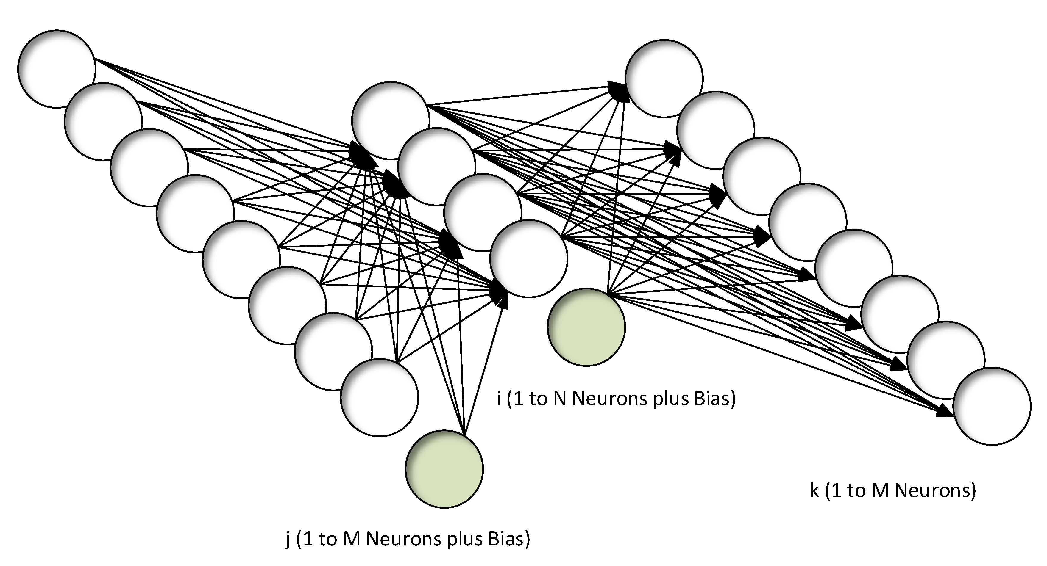
An autoencoder with the same layer structure as the one shown in
Figure 1 is used.
Domain Definition
Here, the encoder layer connection between
j (neuron source layer) and
i (neuron destination layer) is discussed (
Figure 2).
- 1.
Uniform Recurrence Equations
From Equations (
1) and (
2), uniform iterative Equations (
3) and (
4) can be obtained:
where
y stands for activation,
w for weight,
f for the non-linear function, and
j,
i for the indexes in the source and destination layer.
and the boundary conditions:
- 2.
= dependence vectors = { (0,1) (1,0)}
- 3.
D = {(i,j) N i 1 M + 1 j 1 }
- 4.
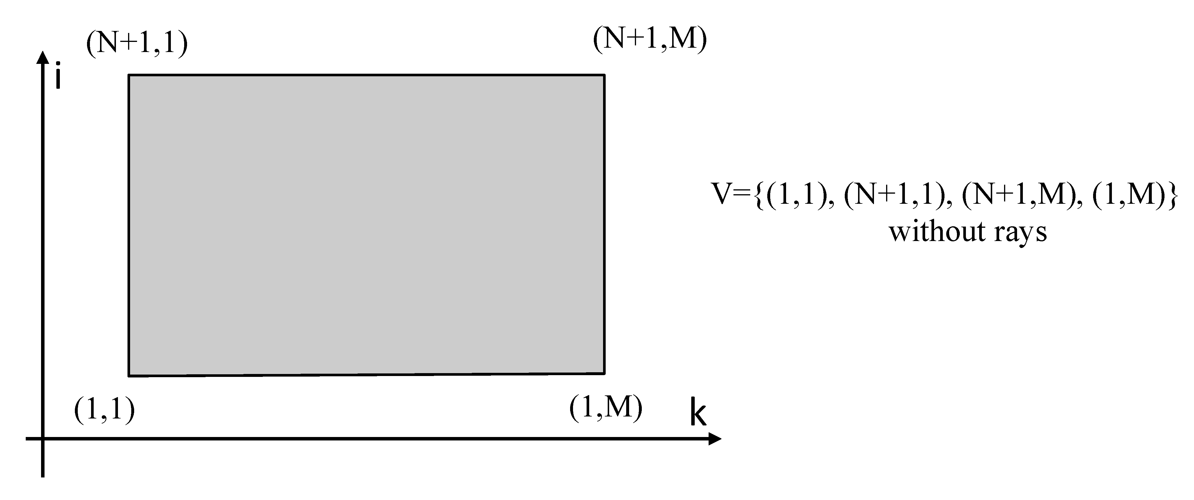
Domain geometry.
The geometry of the domain is shown in
Figure 3.
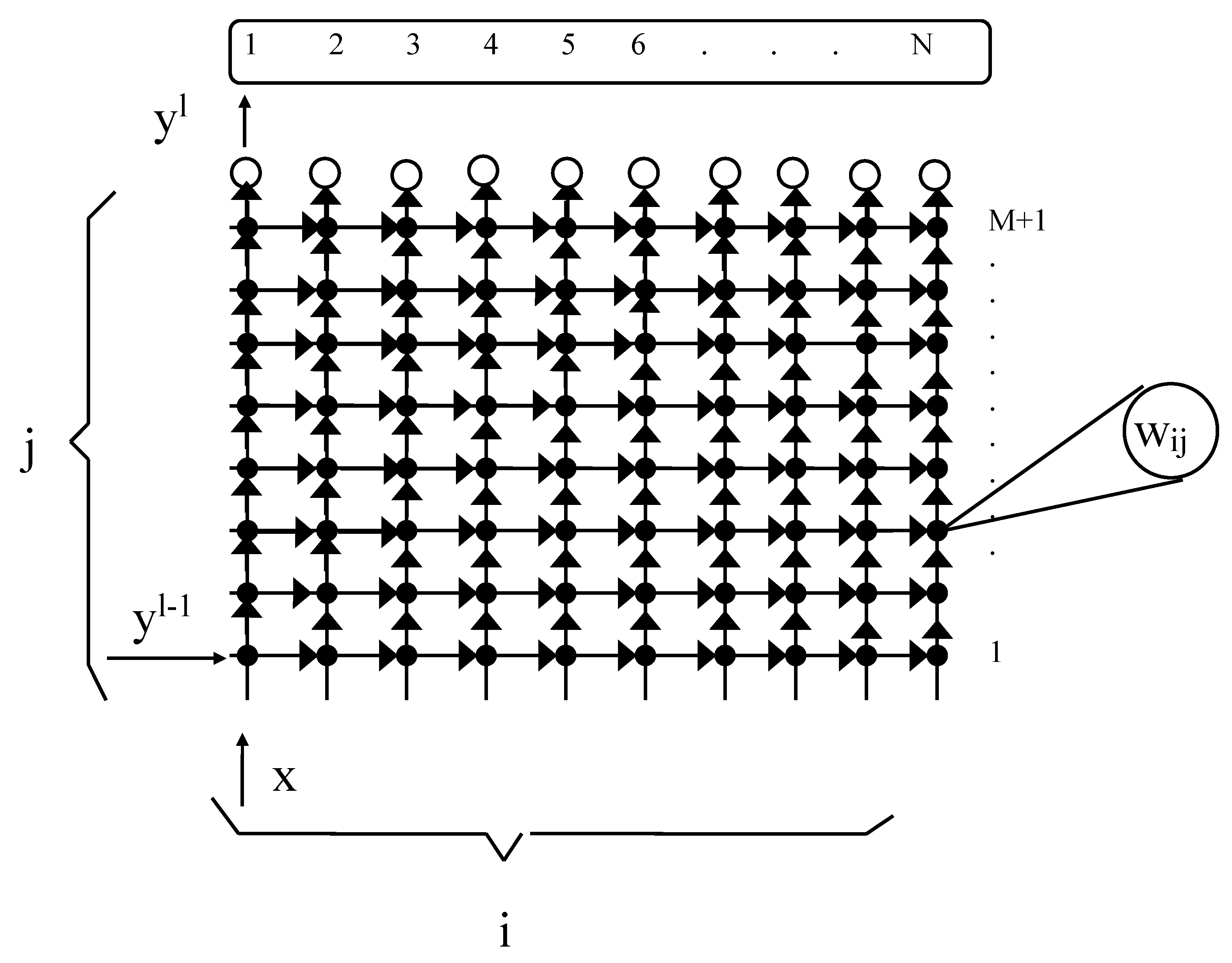
Resulting Systolic Array
The final result of the systolization procedure with a direction (1,0) projection is the systolic array shown in
Figure 4.
The fundamental characteristics of this projection in a interconnection layer are:
- ■
The number of functional blocks, called “vertical synapses”, equals the number of neurons in the source layer. Those functional blocks basically perform the function ; and
- ■
The number of functional blocks (neurons) is 1. This functional block implements the activation function.
3.1.2. Decoder
An autoencoder with the same layer structure as the one shown in
Figure 1 is used.
In this section, the decoder layer connection between
i (neuron source layer) and
k (neuron destination layer) is discussed (
Figure 5).
- 1.
Uniform recurrence equations.
From Equations (
5) and (
6), uniform iterative Equations (
7) and (
8) can be obtained:
where
y stands for activation,
w for weight,
f for a the non-linear function, and
i,
k for the indexes in the source and destination layer.
and the boundary conditions:
- 2.
= dependence vectors = { (0,1) (1,0)}
- 3.
D = {(k,i) M k 1 N + 1 i 1 }
- 4.
Domain geometry.
The geometry of the domain is shown in
Figure 6.
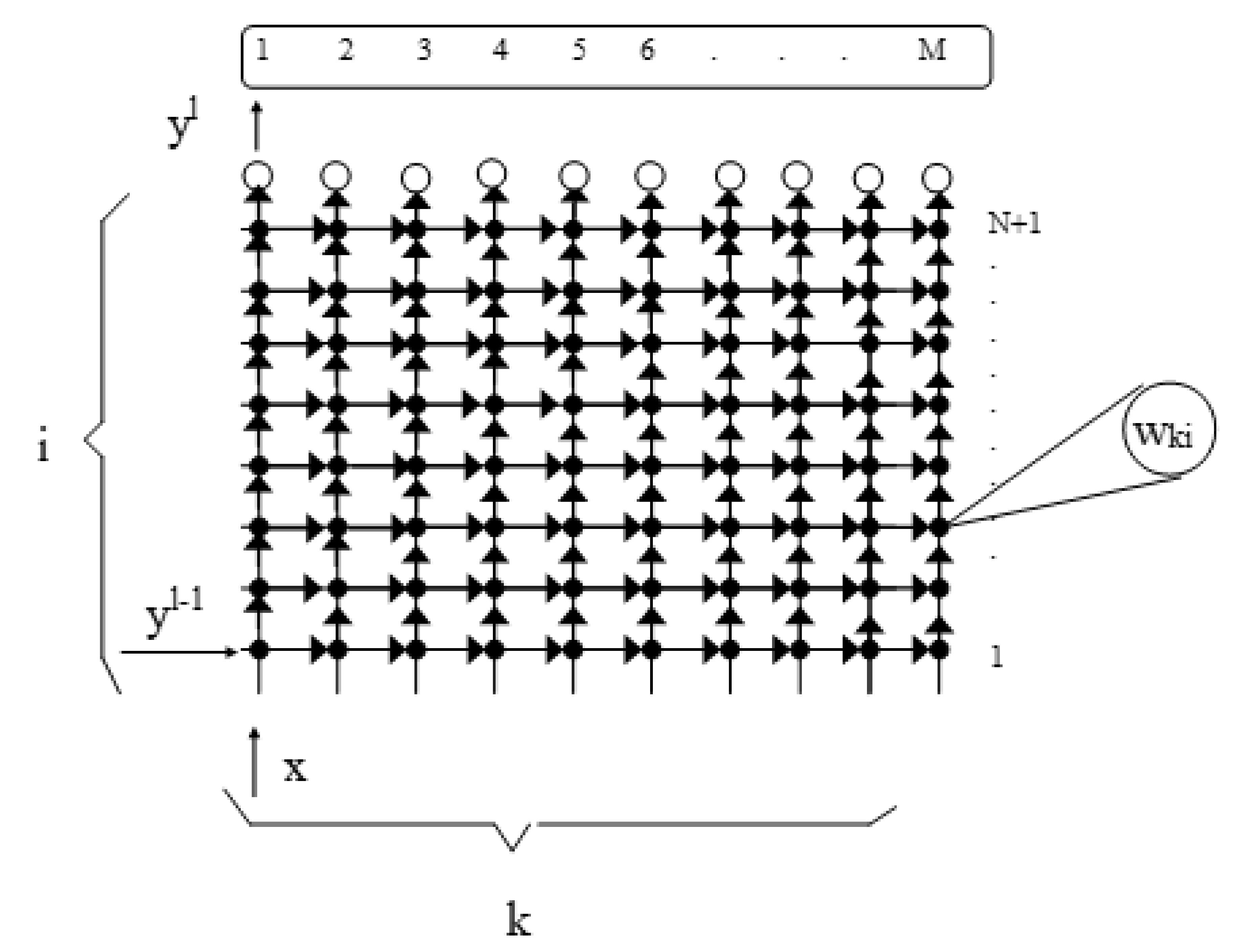
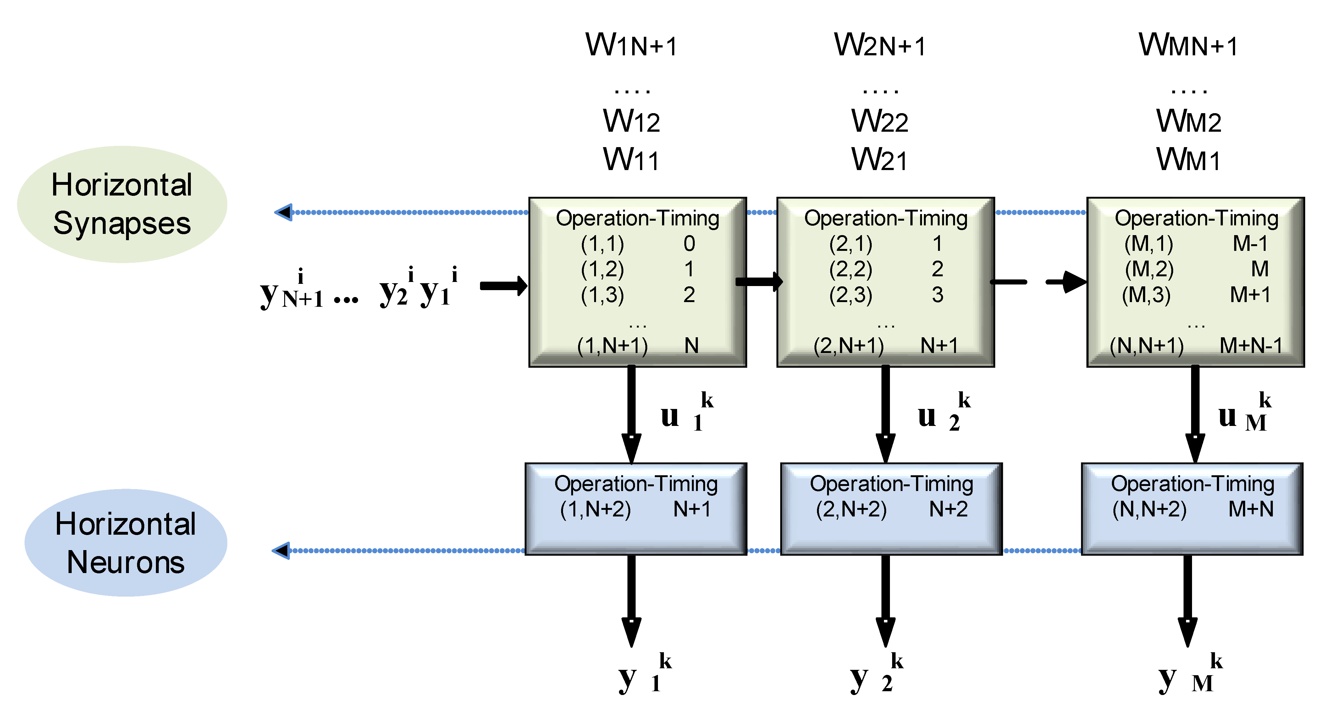
Resulting Systolic Array
The final result of the systolization procedure with a direction (0,1) projection is the systolic array shown in
Figure 7.
The fundamental projection characteristics for an interconnection layer are:
- ■
The number of functional blocks, called “horizontal synapses”, equals the number of neurons in the target layer. Those functional blocks basically perform the function Accu = A × B + Accu; and
- ■
The number of functional blocks (neurons) equals the number of neurons in the target layer. This functional block implements the activation function.
3.1.3. Alternative Architecture
The same study can be repeated by choosing the projection direction (0,1) for the encoder layer and the projection (1,0) for the decoder layer. This choice was made in order to enable an efficient communication between layers.
3.2. Conversion of the Systolic Architecture to OpenCL
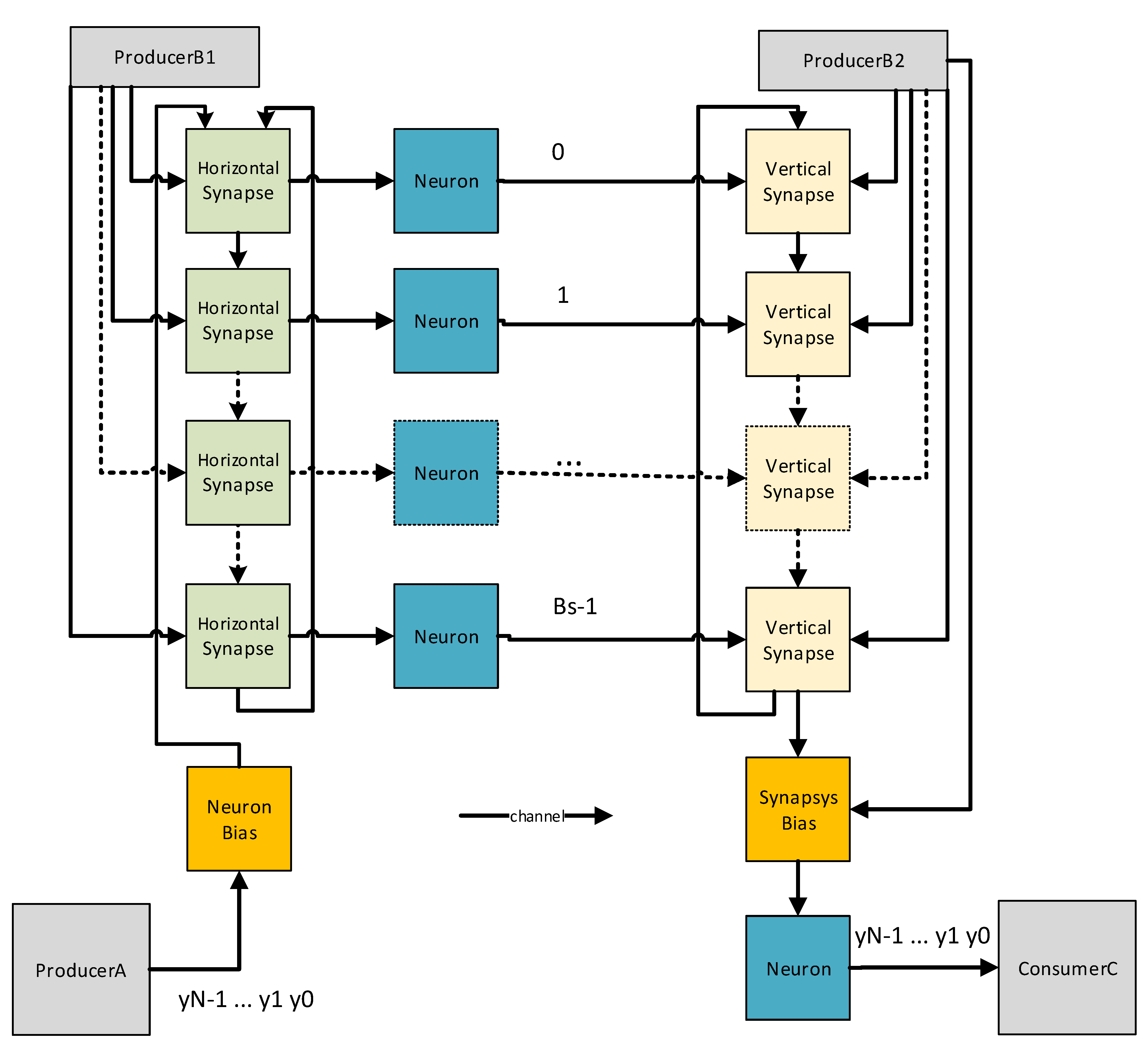
The first proposed architecture (called the V-H architecture here) is shown in
Figure 8.
The second proposed architecture (called the H-V architecture here) is shown in
Figure 9.
As already shown, these architectures are the combination of the encoder and decoder layers discussed in the previous subsection:
- ■
All the data streams were implemented through channels. Those channels perform two important tasks: the transmission of data and control signals and the synchronization of the systolic architecture. Each processing unit (synapses and neurons) can only operate when all of the data and control channels have data available. Otherwise, these processing units are blocked while the queues (channels) are empty. Therefore, all of the processing units (synapses and neurons) act autonomously and do not need to be commanded from the host. The difficulty in this approach lies in making the systolic network adaptable to different numbers of inputs, outputs, and neurons in the hidden layer without having to recompile the OpenCL code. This task is performed by the control generation units, which distribute control commands through the associated channels. Alternative to the latter scheme, in order to improve the performance of the systolic architecture, a distributed control scheme located at each processing unit can be used instead of a centralized one. This results in a loss of flexibility. Since the processing units do not have direct connectivity to the host, it cannot modify the properties of the implemented network by means of arguments.
- ■
The two encoder and decoder layers are constructed based on a BLOCK-SIZE parameter (Bs in
Figure 8 and
Figure 9). The BLOCK-SIZE parameter is used several times to cover the number of inputs and outputs, as shown in
Figure 8, or to cover the number of hidden neurons, as shown in
Figure 9. In the cited experiments, BLOCK-SIZE values of 16, 32, 64, and 128 were considered, which respectively provides 32, 64, 128, and 256 floating point DSPs.
- ■
All the operations are in single precision format.
- ■
Theoretically, an interconnection layer systolic architecture in which the source layer number of neurons is higher than that in the target layer is more efficient when horizontal projection is used. On the other hand, a vertical projection is more efficient when the number of neurons in the target layer is larger than that in the source layer. As a consequence, the architecture shown in
Figure 9 was expected to be more efficient with autoencoders whose hidden layer is smaller than the input layer. This last assumption is experimentally corroborated by means of a 640-256-640 (inputs-hidden-outputs) topology autoencoder configuration in the following sections.
3.3. RTL Refinement
3.3.1. Introduction of the Nonlinear Function inside the Kernel
Our experience in designing backpropagation (BP) algorithm accelerators [
19,
20] along with other works [
21] indicates that one of the most effective means of achieving acceleration is usually to replace the software implementation of the hyperbolic tangent with a hardware one.
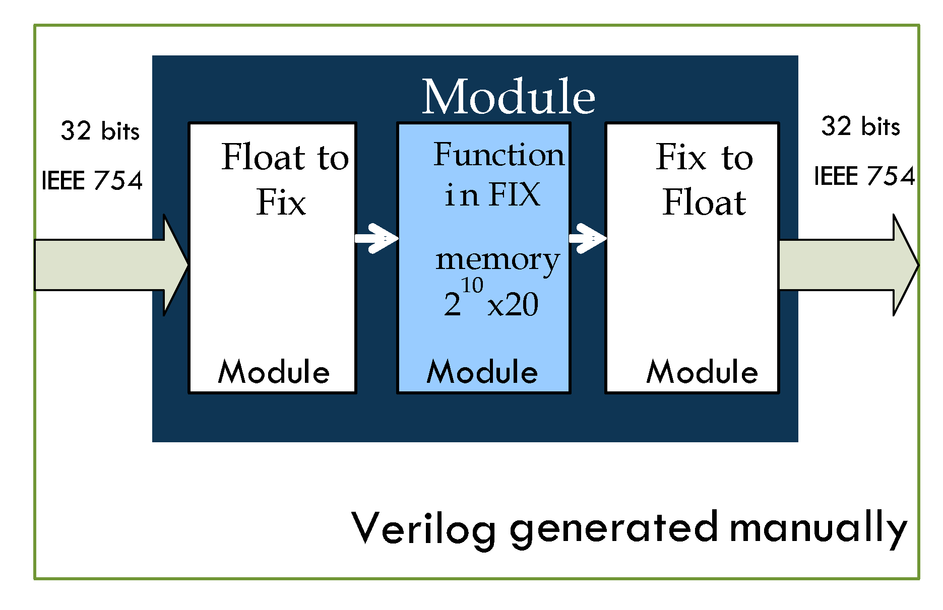
The processing units depicted in
Figure 8, called neurons, necessarily include the nonlinear activation function in OpenCL based implementations. The proposed hardware implementation makes use of lookup tables (LUTs) with a memory capacity that could be implemented using the Arria 10 devices’ embedded memories. An organization of
is used in the proposed implementation.
For instance, when the hyperbolic tangent is used as the activation function, a direct implementation through OpenCL is highly unsatisfactory in terms of area and speed, as shown in
Table 1.
As seen in Equation (
9), the substitution of the hyperbolic tangent by some of its equivalent formulas can be a better implementation. Results from Expression 3 are shown in the second row of
Table 1. Bearing in mind that a systolic architecture with BLOCK-SIZE = 16 would need to replicate 17 times the results shown in
Table 1, the final area would be unacceptable.
Our results regarding the resources being used and speed performance (latency) are shown in the row labeled “RTL tanh IP” in
Table 1. This approach is outstanding in terms of area and speed; moreover, it has no impact on the recall work mode of the trained autoencoder from the precision point of view.
Therefore, we attempted to insert our own Verilog RTL code in place of the current standard implementation of the hyperbolic tangent function in OpenCL (see
Figure 10).
3.3.2. Instantiation of DSPs versus Direct Inference
The same procedure used for the implementation of hyperbolic tangent functions inside PPE neurons was applied to PPE synapses in order to achieve further refinement based on register transfer logic (RTL) libraries written in Verilog-SystemVerilog.
Results in
Table 2 demonstrate that for the
function’s implementation, the RTL code based instantiation versus OpenCL code inference has no remarkable impact in terms of efficiency. However, in the case of function
, the amount of resources saved by using direct instantiations of horizontal synapses is remarkable (
Table 3). An overall improvement in both area and performance can be observed for autoencoder implementations with 256-640-256 and 640-256-640 topologies (
Table 4 and
Table 5).
4. Performance Evaluation
The Arria 10 family was specifically introduced as the technological answer of the FPGA world (by the manufacturer IntelFPGA) to manage floating point operations and that could compete with GPUs. It is important to demonstrate in our article that the DSPs of this technological family can be handled more efficiently than the automatic inference performed by the OpenCL base compiler. This led to the development of their own libraries based on Verilog RTL code and the management of their development tools for new compilation libraries provided by the manufacturer. Of course, the development of these libraries requires being able to demonstrate with different devices of the same family that this proposed refinement is still working without problems. That is why we carried out an intensive study of the behavior of several boards with this technological family of FPGAs (
Section 4.1,
Section 4.2 and
Section 4.3). It is also important to demonstrate the importance of communication between layers (observed mainly in the throughput study in
Section 4.2) and host communication with the existing multikernel inside the FPGA (observed mainly in the latency study in
Section 4.3).
4.1. Throughput and Latency Measurements
The process performance can be measured in two different inference ways: synchronous or asynchronous. In the asynchronous case, multiple requests are typically executed asynchronously, and the performance is measured in frames per second (fps), dividing the number of images being processed by the processing time. For latency-oriented tasks, the time to process a single frame is more important.
These measures offer comparative information between architectures and are usually provided by environments like OpenVINO as standard performance measurements.
However, it is important to clarify the following points regarding these results:
- 1.
The autoencoder topology being used is 640-256-640. The sizes of the input and output are determined by our needs in medical imaging application where autoencoders are required.
- 2.
Four board support packages (BSPs) for the IntelFPGA Arria 10 family of devices were used. The manufacturers of these BSPs and boards are:
- ■
Alaric Arria 10 (Reflex CES) and Alaric Arria 10 (Reflex CES) with the support of host pipes [
22].
- -
4 GB DDR3 on-board memory.
- -
PCIe Gen3 x4.
- -
FPGA: Arria 10 SX: 660 K logic elements, 1688 hardened single-precision floating-point multipliers/adders (MACs), speed grade-2.
- ■
- -
8 GB DDR4 on-board memory.
- -
PCIe Gen3 x8. PCI passthrough.
- -
FPGA; Arria 10 GX: 1150 K logic elements, 1518 hardened single-precision floating-point multipliers/adders (MACs), speed grade-2.
- ■
- -
8 GB DDR4 on-board memory.
- -
PCIe Gen3 x8.
- -
FPGA: Arria 10 GX: 1150 K logic elements, 1518 hardened single-precision floating-point multipliers/adders (MACs), speed grade-2
- 3.
BSPs describe system architectures that include a host and an accelerator connected through a peripheral component interconnect (PCI) express bus. The host sends the image matrix (each image occupies a row of the matrix) and receives the reconstructed images generated by the autoencoder (each row occupies a row of the matrix of reconstructed images).
- 4.
In our medical imaging applications, a 10 s throughput specification is required. This requirement must be fulfilled by a parallel set of six FPGAs. The results obtained in this work show a 11.13 s throughput for a single FPGA. Therefore, using a proper parallelization method, the initial throughput specification could be fulfilled.
- 5.
Networking-type solutions could also be applied to our medical imaging applications. These solutions can deal with up to 10 G data networking connections in which the fundamental communication element would be the Standard 10 G low latency MAC IP (Intel/Altera).
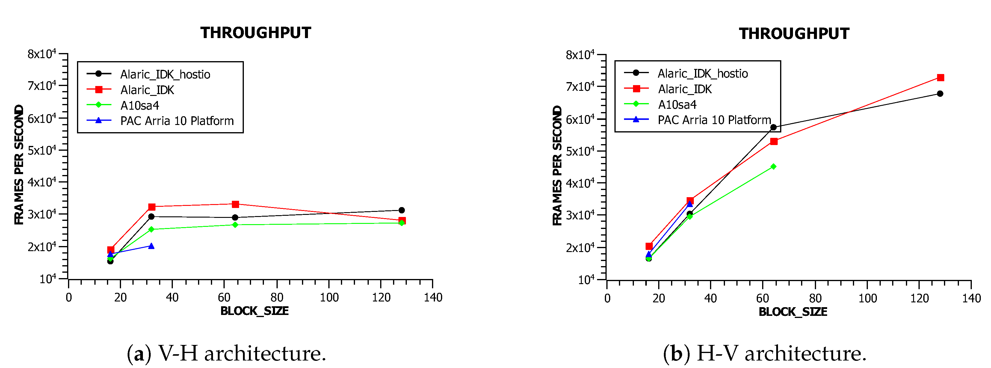
4.2. Throughput Results
A close look at the throughput results (
Figure 11a,b) supports our hypothesis that the H-V architecture represented in
Figure 9 is more efficient than the V-H architecture shown in
Figure 8. This is a direct consequence of the underlying architectural properties inherited by the OpenCL implementation.
To further corroborate this hypothesis, an autoencoder with opposite characteristics to those required for our experiments was also implemented. The new autoencoder topology consists of a hidden layer larger than the input and output layer (256-640-256). The throughput results in
Figure 12a show that efficiency with the H-V architecture is higher than with the V-H architecture for the 640-256-640 topology. As shown in
Figure 12b, the efficiency with the V-H architecture is higher than with the H-V architecture for topology 256-640-256.
For an optimal architecture topology, a higher (BLOCK-SIZE) parameter value improves the throughput. This result was expected as the number of DSPs involved is increased by the same amount. However, efficiency per DSP shows a falling tendency, since a higher complexity decreases the maximum frequency of operation.
Regarding the different board support packages (BSPs) being used (associated with different boards), our intention was to demonstrate the adequacy and robustness of the systolic architecture rather than to establish a comparison among them. Those systolic architectures were implemented on different boards with different versions of the OpenCL compiler. In asynchronous inference mode, the use of host pipes was not decisive.
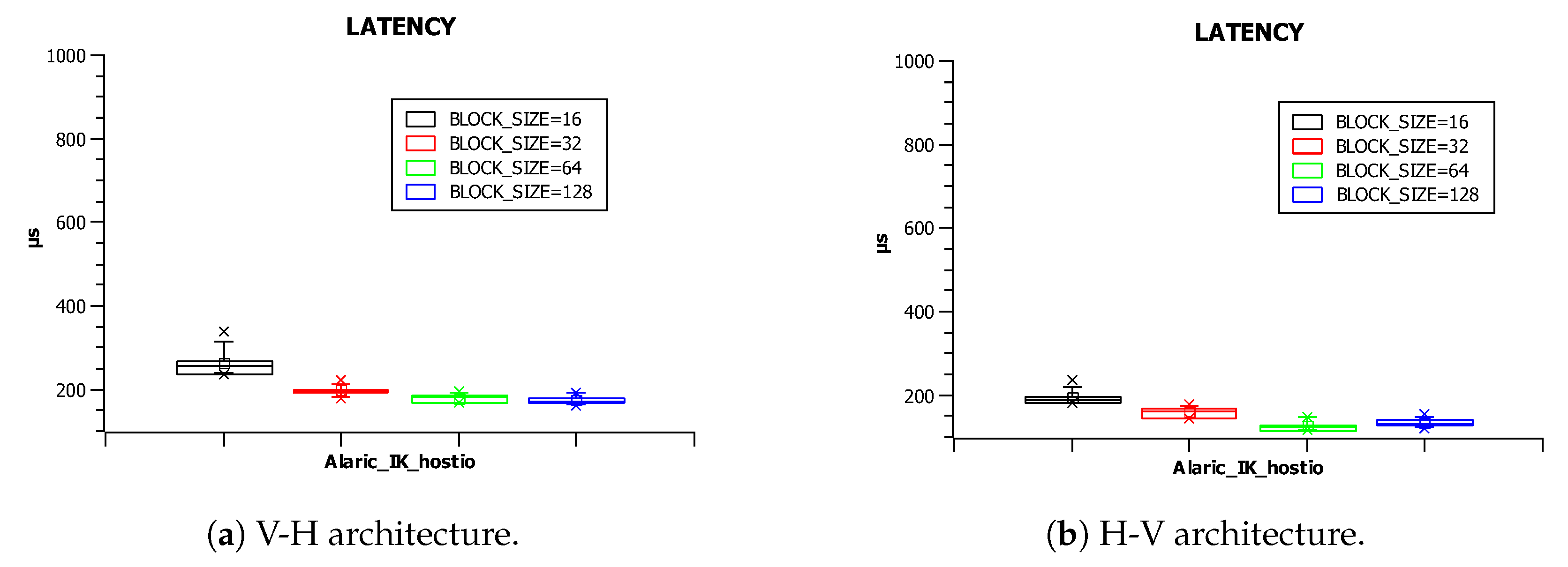
4.3. Latency Results
Regarding the latency results, the most remarkable conclusion is that such latency is hardly dependent on the architecture being used (compare
Figure 13a,b) and slightly dependent on the BLOCK-SIZE parameter value (shown in
Figure 14a,b,
Figure 15a,b,
Figure 16a,b and
Figure 17a,b).
Communication between the host and kernels, which receive the input data and transmit the output results back to the host, has the strongest impact on the latency. Some BSPs are able to implement host pipes, which allow the lowest latencies.
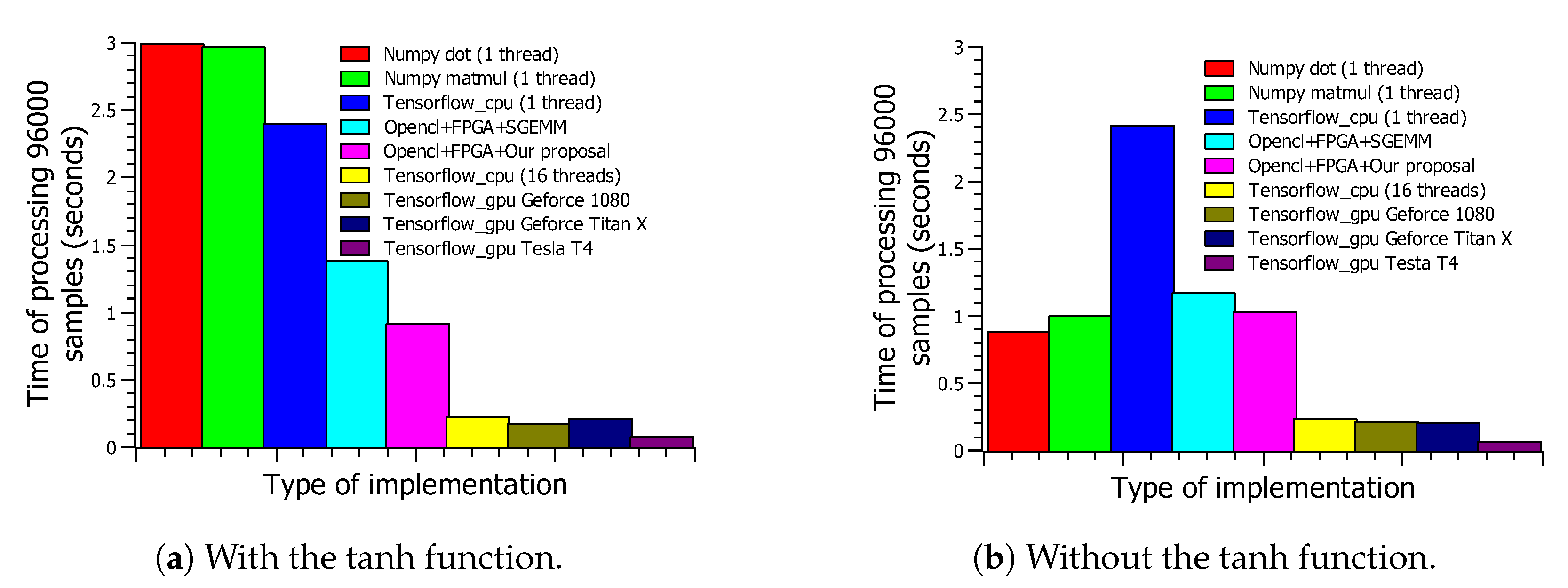
4.4. Comparison of the Implementations
In this subsection, our autoencoder based systolic architecture processing speed is compared to other implementations: CPU, GPU, and FPGA solutions based on the single float precision general matrix multiply (SGEMM) implementation.
Figure 18a,b shows the speed performance of our proposal compared to other hardware and software implementations. The GPU based implementations are the most efficient and virtually share the same degree of flexibility with CPU based implementations. The implementation platform was Tensorflow Version 2.2.
Regarding FPGA based hardware accelerators, the differences are no longer so evident (
Table 6 and
Table 7). Neither of the implementations reach the specified throughput (10
s per image or 100,000 fps). However, both reach those specified constraints if we eliminate the communication times between the host and kernel. The execution time of the internal kernel of the FPGA is less than 0.96 s in both cases. The performance of the internal kernel based on single float precision general matrix multiply (SGEMM) (
Table 7) is even better than our implementations. However, the computational efficiency must be taken into account. In SGEMM based solutions, the number of DSPs used is four times higher than in our systolic architecture. Therefore, its computational efficiency (GOP/s/DSP) is worse than that of our proposal.
Finally, there is another key point regarding both implementations: our proposed method can work with any number of input images, whereas the SGEMM implementation must work with a BLOCK-SIZE multiple number of input images (in this case, 128). In order to get the shortest time in a previously trained neural network recall phase, implementations that can only work with batches of input images should be avoided.
4.5. Discussion
The following aspects from the obtained results can be highlighted:
- ■
GPU based implementations are difficult to beat in terms of neural network inference. We do not aim at comparing ours with such implementations, but to use them as reference points for FPGA based implementations. In terms of throughput performance for 32 bit floating point resolution implementations, GPUs beat FPGAs by a wide margin.
- ■
With OpenCL based hardware implementations on FPGAs, a greater computational efficiency can be provided by using systolic architectures. We wanted to achieve an intermediate point between the use of HLS and HLD that would result in a flexibility close to that of HLS solutions and would improve performance. Although this was achieved, there is still a long way to go in improving OpenCL compilers, especially in the resources used for channel synthesis, accumulator synthesis, and non-linear function synthesis.
- ■
Comparing among the FPGA implementations, we have lower performance when using HLS. We selected [
13] as a reference implementation with similar characteristics as ours. This reference claims a 3.24
s throughput autoencoder of size
and an 18 bit fixed point resolution. Their authors made use of a ReLU (rectified linear unit) for the activation function implementation as a performance enhancement. In our case, a 9.47
s throughput was achieved with a 32 bit floating point resolution using a hyperbolic tangent as the activation function.
- ■
From the point of view of the ease of design, we cannot experimentally quantify this ease with respect to the use of HDL. We carried out HDL based implementations, as well as HLS (OpenCL) ones, though it is difficult to get a design time estimation. Moreover, there is a lack of references in the bibliography regarding this parameter. However, we claim that the creation of these systolic architectures in OpenCL with multikernel can even be automated as we already did with experiences starting from c++ and having as a destination a single-work-item-type kernel [
25].
5. Conclusions
In this paper, a workflow for the implementation of deep neural networks was proposed. This workflow tries to combine the flexibility of HLS based networks and architectural control features of HLD based flows. The main tool used along the workflow was OpenCL. This system level description language allows a structural approach, as well as a high degree of control from a hardware point of view. This fact is of main importance when dealing with systolic architectures.
Following the described methodology, the performance obtained is encouraging, and the design times could be shorter provide that in the future, we could automate the generation of OpenCL from the frameworks used in machine learning. As far as the architectures are concerned, the proposed workflow could reuse classic VLSI architectural solutions or introduce new ones.
The connection between layers was shown to be a crucial issue that must be carefully studied in deep neural network implementations. A failure in choosing the right combination of projections may lead to a considerable loss of performance. The challenge is to be able to work with larger images, trying to process more than 100,000 frames per second, working with a networking-type source and destination.
Although this work focused on simple neural networks (autoencoders), our intention for future research is to extend these conclusions to interlayer communication techniques on higher complexity neural networks such as CNNs.

 ,
, 


