1. Introduction
Soil moisture represents a vital component of the ecosystem sustaining life-supporting activities at micro and mega scales [
1,
2]. It is highly variable with spatial and temporal scales and depends upon the topographical, soil, land cover and climatic conditions [
3,
4]. Thus, soil moisture is an integral part of the hydrological cycle and is essential for human and plant growth [
5,
6,
7]. Measurement of this parameter is imperative to agricultural aspects due to its importance for early monitoring of drought warnings. Land use and land cover influence soil moisture spatiotemporal variability and can alter soil hydraulic properties because of changes in porosity and structure of the soil [
8]. Soil moisture assessment in the root zone controlling the crop productivity provides information for deficits in soil moisture [
9]. Hence, regular soil moisture monitoring provides appropriate irrigational facility to improve crop productivity and yield forecasting. Furthermore, soil moisture provides information, prediction and forecasting on flood before rainstorms. At the saturation level of soil, floods will likely to occur during the event of rain as its capacity to hold water has reached a limit and thus is unable to absorb an adequate amount of water [
10,
11,
12]. Among others, Reference [
13] stressed the importance of soil moisture information for meteorologists, since this parameter is related to weather changes, thereby providing a more accurate weather forecast. In addition, information on this parameter is important in biodiversity and ecosystems management [
14].
These applications mentioned above show the importance of soil moisture at local, regional and global scale. Thus, precise, accurate and adequate knowledge on soil moisture at different scales is essential for agricultural crop productivity, flood monitoring and soil conditions/status. However, the lack of information on soil data at different scales for large regions is still an issue due to its extreme variability in both the spatial and temporal domain and at different observation scales. Soil moisture can be directly measured using wide range ground instruments [
15]; yet, such approaches cannot fully describe the spatial and temporal variability of soil moisture at larger scales. On the other hand, remote sensing techniques have the advantage of achieving simultaneously satisfactory sampling frequency and global coverage [
7,
16,
17]. Nonetheless, most of the relevant operational products available today are providing soil moisture at coarse resolution. To acquire high spatial resolution soil moisture at regional and local scales, spatial interpolation and GIS can play an important role. Spatial interpolation and GIS emerged as powerful tools in remote sensing technology demonstrating their capability to provide spatial continuous data required for environmental monitoring [
18].
For estimation of attribute values at unsampled location, spatial interpolation of in-situ measurements from sampled locations is necessary to achieve continuous spatial data. This necessity is added when the discrete surface has a different spatial resolution, cell size or orientation as required, when the continuous surface is represented by a data model other than required and when the available datasets do not cover the regions of interest completely [
19,
20]. In these instances, spatial interpolation methods act as a solution and provide continuous data at the unsampled sites (unknown locations) by estimating environmental variables from point observations within the same region [
20]. Several spatial interpolation as well as extrapolation methods were developed and applied in different research disciplines including geo-statistics [
21]. There is a variety of such methods which are proposed as more suitable in each case according to the specific data types or specific variables to be interpolated. Thus, is difficult to assign spatial interpolation methods as the “best practices” based on a given datasets without a prior investigation of their accuracy [
22]. However, spatial interpolation has a profound impact on several factors including sample size, sample design and the nature of the data. Moreover, the predictive performance of the method were not consistent as shown in previous studies, while as the variation increases, the accuracy of all methods changes either increases or decreases [
23]. Yet, there is no proved consistent findings about variation and how the previously mentioned factors affect the performance of the spatial interpolation methods. Therefore, it is difficult to select an appropriate spatial interpolation method for a given specific input dataset due to variation within the data [
20].
There have been some research studies focusing on interpolating soil moisture [
22,
24,
25,
26,
27]. For example, [
22] demonstrated that ordinary kriging and Inverse Distance Weighting (IDWmethods employed for the estimation of soil moisture at complex terrain results in poor performance due to low spatial autocorrelation of soil moisture at small catchment scale [
24,
25,
28]. Another study [
27], compared different interpolation methods (inverse distance weighting, multifarious forms of kriging, regularized spline with tension and thin plate spline) for estimating soil moisture in an area with complex topography in southwest China. Their results indicated that inverse distance weighting had the best performance, at least this was the case in their study.
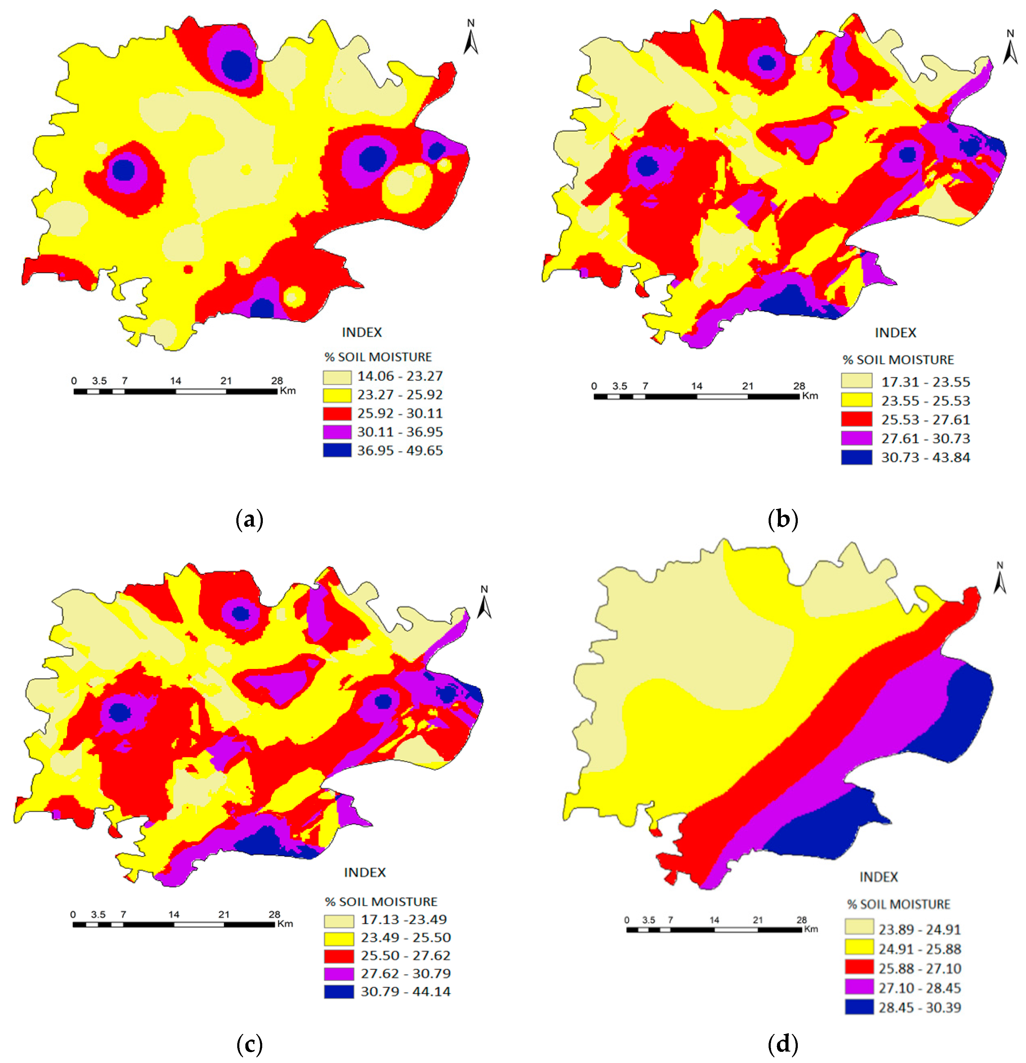
The present study builds on studies such as the above, aiming at developing a geo-spatial database for soil moisture at district level and assessing a range of widely used spatial interpolation techniques for soil moisture estimation using GPS-aided information. Four spatial interpolation methods, namely Inverse Distance Weighting (IDW), Spline, Ordinary Kriging models and Kriging with External Drift (KED) are compared in estimating soil moisture. As a case study, Varanasi city located in India is used, and for this region to our knowledge for the first time a soil moisture destitution map is developed for the area taking into account all the particular environmental characteristics of the region. An additional added value of our study is also the use of remote sensing techniques to define Digital Elevation Model (DEM) and Land Cover maps and the incorporation of soil organic carbon information as a secondary variable.
2. Materials and Methods
2.1. Study Area
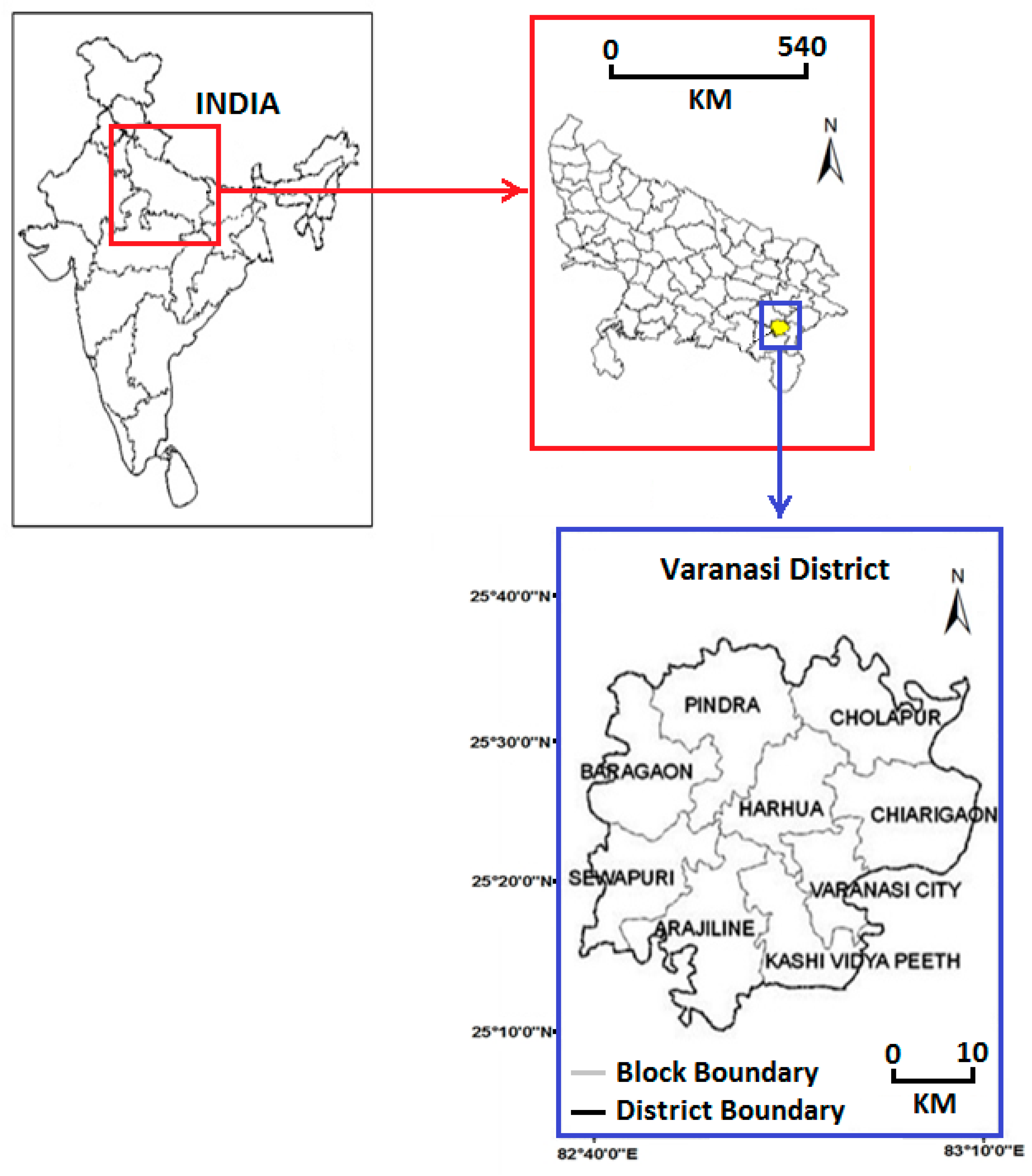
The study area chosen is Varanasi City, India. The study area extends from 25°10′3″ and 25°35′1″ N to 82°40′5″ and 83°12′1″ E. It covers a total area of 1535.00 km
2 which 1371.22 km
2 is under rural land and 163.78 km
2 is under urban land and it is elevated above mean sea level at 80.71 m (
Figure 1). The River Ganga here flows south to North, having the highest flood level at 73.90 m (1978) and the lowest river water level is approximately 58 m. It is a part of Indo-Gangetic plain covering parts of alluvial deposit of river Ganga and Varuna makes the favorable conditions like fertile soil, plain topography for settlement, availability of fresh water have intense bearing on the high population density along with the historical development of the town as an oldest pilgrimage city in India. It consists mainly of sand, silt and clay interspersed by pellets stones at a few places nearby rivers. Climatically the region has sub-tropical monsoonal climate characterized by seasonal extremities. It has humid sub-tropical climate and experiences large variation between summer and winter temperatures. The total annual precipitation is 10,582 mm and humidity is ~70% and mean maximum annual temperature is ~32 °C and mean minimum annual temperature is ~19 °C. The studied area is situated on the crescent shape bank of perennial river Ganga up to a stretch of 2525 km
2 which has high seasonal variations in discharge due to monsoonal impact.
2.2. Datasets and Methodology
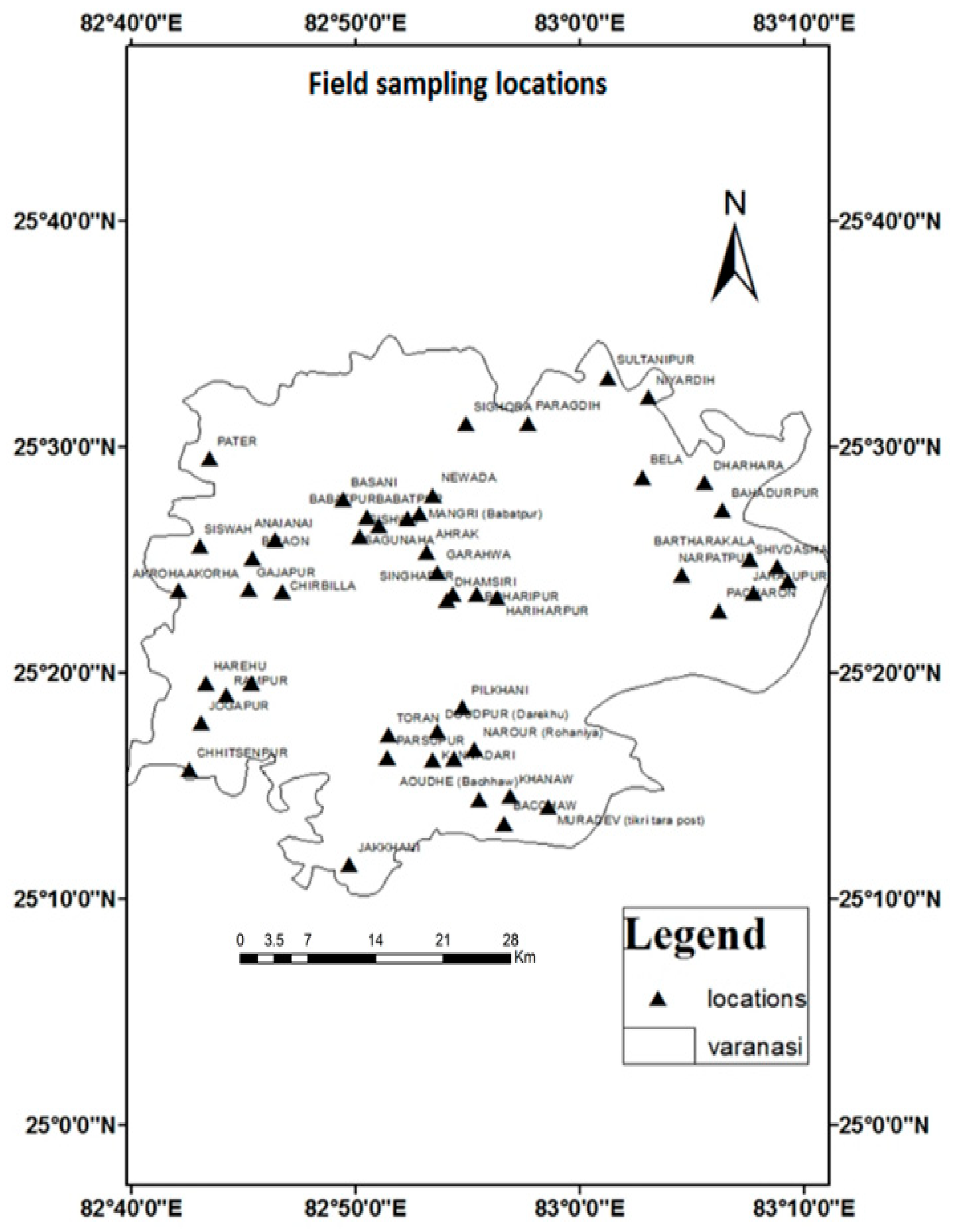
The entire Varanasi district, including nine district blocks, namely, Varanasi City, Arajiline, Sewapuri, Baragaon, Pindra, Cholapur, Harhua, Chiraigaon and Kashi Vidya Peeth (KVP) was surveyed to collect soil samples with 5 cm diameter core pipe and up to the depth of 5 cm and 20 cm from the surface. From each block, 10 locations were chosen randomly for consideration with a horizontal distance of 5 to 9 km among locations and in different directions. The Varanasi city block was excluded from sample collection as it is a fully urban area. Major soil samples were taken from paddy fields and some sample points from barren land and plantation area because this study has its main focus on soil moisture and its related attributes so non-arable lands are of less importance. The entire fieldwork was completed during the months of August and September 2015 for a total of 82 locations (
Figure 2). Out of the total 82 locations, 54 locations data were used for calibration and 28 locations data was used for validation following the thumb rule of 2/3 for calibration and 1/3 for validation. Soil moisture (in % of vol. vol.
−1) data on field for every location was measured by Stevens Hydraprobe at 5 cm and 20 cm depths. GPS (global positioning system) was used to record coordinates of every location that was used further in map processing in GIS. The data processing and analysis was worked with ArcGIS v10.1 (ESRI, Redlands, CA, USA) and ENVI v5.2 (Exelis, Boulder, CO, USA). Statistical analysis was performed using spatial analyst of ArcGIS v10.1, RStudio platform and Microsoft Excel packages.
Soil moisture was estimated using mean values from soil moisture measurements that took place at the above mentioned 82 locations of the study area. The soil moisture measurements took place daily during the months of August and September of 2015. Also, in the studied interpolation techniques, for each location, the mean values of soil moisture at the two different depths (5 and 20 cm) were used as input.
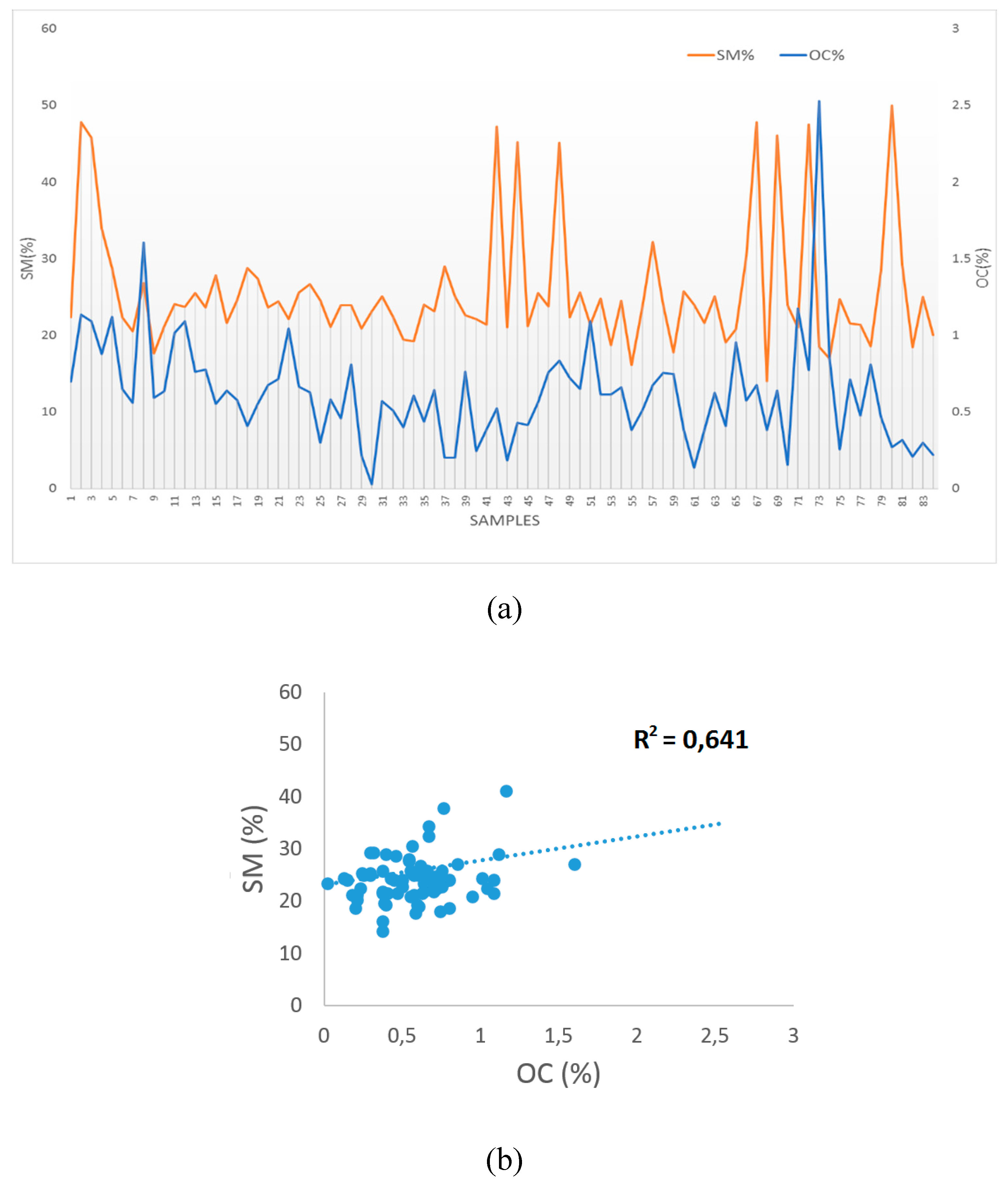
In addition, the above mentioned 82 soil sampling locations were used to obtain the appropriate information regarding the soil organic carbon. In turn, soil organic carbon information was incorporated in KED interpolation method as a secondary variable. Also, in this study a series of statistical metrics (Percent bias (%Bias), root mean square error (RMSE), mean absolute error (MAE)) were utilized in order to determine the performance of the different interpolation models.
2.3. Methodology
2.3.1. Soil Moisture and Organic Carbon Estimation
In this study, soil moisture measurements were conducted using the Stevens hydraprobe. This provides a measurement of the average volumetric water content along the length of the waveguide. Among the most important advantages of this technique are that it is non-destructive to the study site and is not labour intensive [
29,
30].
The amount of organic carbon present in the soil samples was determined applying the Walkley-Black chromic acid wet oxidation method. The oxidisable organic matter in the soil is oxidized by 1N K2Cr2O7 solution to estimate soil organic carbon. For preparation of 1 N (normality) Potassium dichromate solution, 49.040 g of K2Cr2O7 was dissolved in the deionized water and then the volume of the volumetric flask was made to 1 litre. Second solution was prepared for 0.4 N ferrous ammonium sulphate. 0.4 N ferrous ammonium sulphate solution, 112 g of FeSO4 (NH4)6·7H2O was dissolved in 800 mL of deionized water. Then, 15 mL of concentrated H2SO4 was added to facilitate proper dissolution. Following this procedure, the volume of the solution was made to 1 litre and thereafter, the solution was stored in a dark bottle.
The soil sample was crushed and filtered using a 0.42 mm sieve followed by drying in the oven. Thereafter, dried weighted soil sample was transferred to a 250 mL Erlenmeyer conical flask. 10 mL of potassium dichromate was added to the dried soil followed by gentle swirling to allow proper mixing of the solution with the soil. Then, 20 mL of concentrated H
2SO
4 was added to the soil solution. Following this it was allowed to stand for 1 hour for its proper digestion. Then 200 mL of distilled water was added and allowed to cool. It was then mixed with 2 drops of diphenyl indicator and titrated against 0.4 M ferrous ammonium sulphate. Before analysing the samples, a blank was tested and titrated against the same. The amount of organic carbon in the soil samples was calculated using the following formula (Walkley-Black chromic acid wet oxidation method):
where; N is the normality of K
2Cr
2O
7 solution, T is the volume of FeSO
4 used in sample titration (mL), S is the volume of FeSO
4 used in blank titration (mL) and ODW is the oven-dried sample weight.
The soil organic carbon was estimated using mean values from soil organic carbon analysis-measurements that took place at the above mentioned 82 soil sampling locations of the study area (complex samples at two different soil depths 5 cm and 20 cm for each location). The sampling campaign took place during the months of August and September of 2015. In turn, the mean values of the soil organic carbon for each of the 82 locations were used as a secondary variable in KED interpolation method.
2.3.2. Digital Elevation Model (DEM)
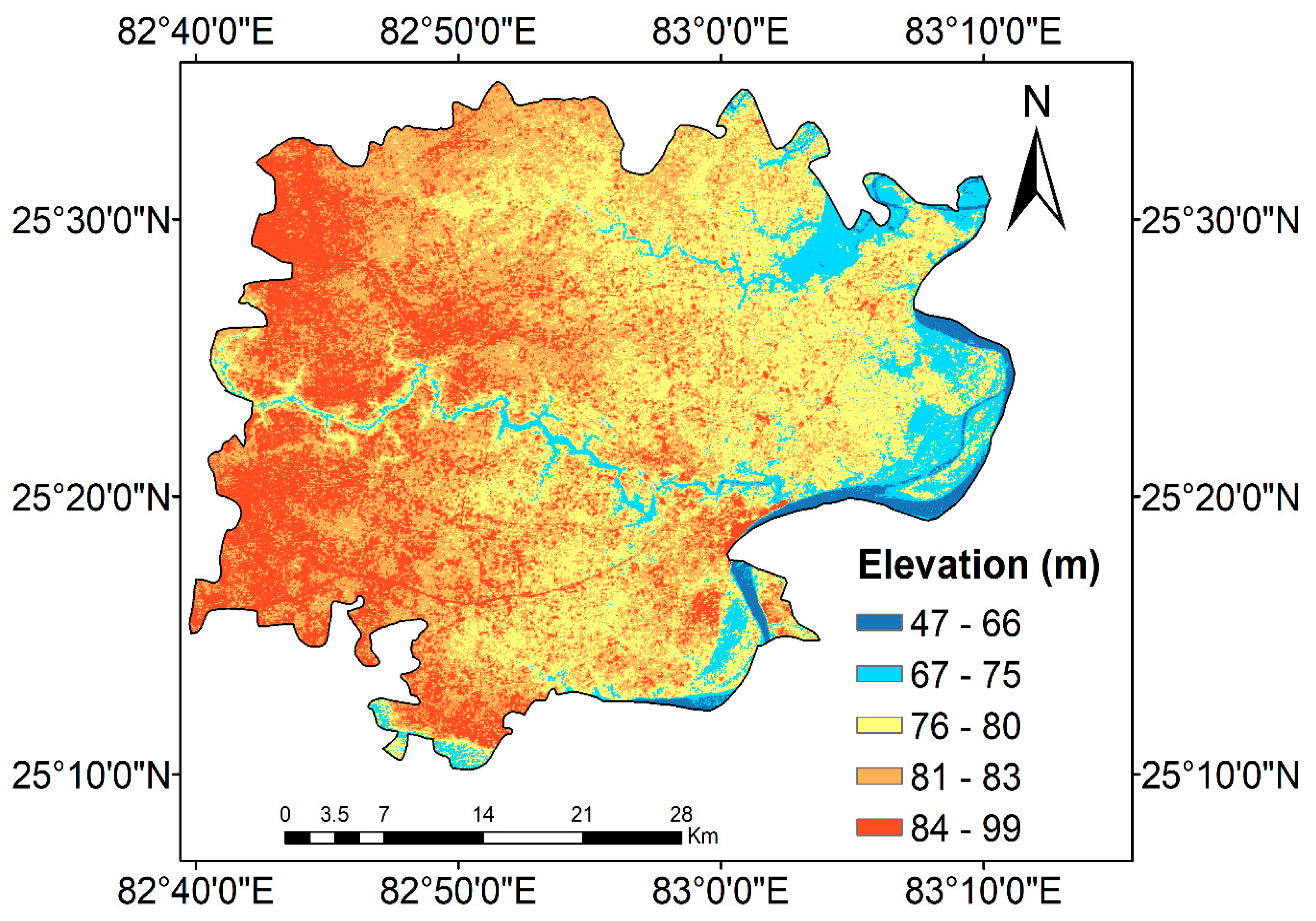
A DEM helps in the demonstration of the topographic data and plays an important role in the modelling and prediction of floods [
31]. DEM involves data in a geodetic coordinate system that is in longitude and latitude. The Shuttle Radar Topography Mission (SRTM) digital elevation data, produced by NASA (The National Aeronautics and Space Administration) originally, is a major breakthrough in digital mapping of the world, providing a major advance in the accessibility of high quality elevation data for large portions of the tropics and other areas of the developing world. The SRTM 90 m DEM provided in mosaicked 5° × 5° tiles was used in this study. The vertical error of the DEM’s is reported to be less than 16 m. In our study, the DEM of SRTM was downloaded from earth explorer official website which is easily available online after minimum formalities.
2.3.3. Database for Land Use Land Cover
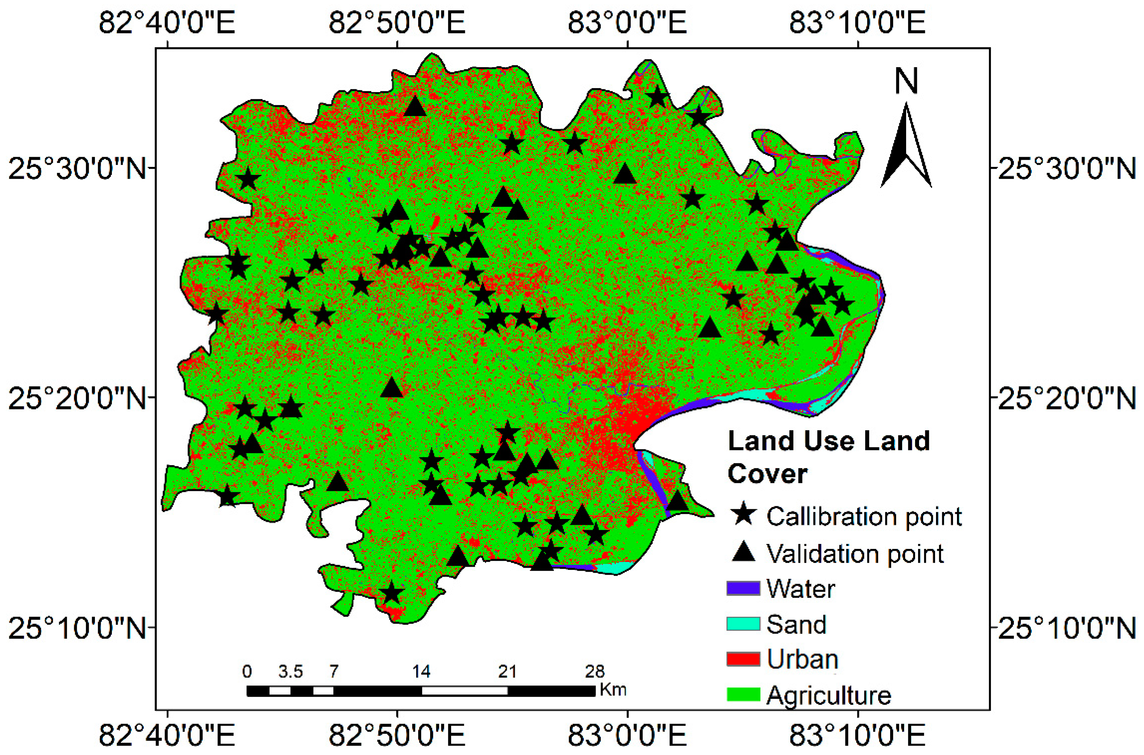
The Landsat images were downloaded from the United States Geological Survey (USGS) portal (
http://www.usgs.gov/). Landsat 8 (L8) data was incorporated with the study of image classification with total eight bands. L8 was launched in 2013 and it has Enhanced Thematic Mapper (ETM+) sensor, 185 km swath, 8 bits, SWIR 30 m and TIR 60 m. World Geodetic System 1984 (WGS84) was used for geocentric reference (
Table 1).
2.3.4. Image Classification
Following the data acquisition, bands stacking and image subset was applied to the images to facilitate computational efficiency in data handling. After this step, land use/cover classes to be included in the classification maps were decided and representative training sites for each of those classes were selected. Approximately 150 pixels per class (600 total pixels) were selected from homogeneous areas. The separability of the selected training points for all cover classes were examined in ENVI (v 5.2, Exelis, Boulder, CO, USA) software. Then, a pixel based supervised image classification that is, Support Vector Machine with Radial Basis Function (SVM RBF) [
32,
33] was implemented to the acquired Landsat images in ENVI using the selected training data. SVMs can produce accurate and robust classification results on a sound theoretical basis, even when input data are non-monotone and non-linearly separable. So, they can help to evaluate more relevant information in a convenient way. Since they linearize data on an implicit basis by means of kernel transformation, the accuracy of the results does not rely on the quality of human expertise judgment for the optimal choice of the linearization function of non-linear input data. SVMs operate locally, so they are able to reflect in their score the features of single companies, comparing their input variables with the ones of companies in the training sample showing similar constellations of financial ratios. Although SVMs do not deliver a parametric score function, its local linear approximation can offer an important support in recognising the mechanisms linking different financial ratios with the final score of a company. For those reasons SVMs are regarded as a useful tool for effectively complementing the information gained from classical linear classification techniques [
34].
2.4. Spatial Interpolation Methods
There are several methods developed for spatial interpolation in various disciplines with a number of different terminologies used to distinguish them, including “interpolating” and “non-interpolating” methods or “interpolators” and “non-interpolators” [
35]. The spatial interpolation methods covered in this study focuses on four methods namely IDW, spline, kriging and linear spatial interpolation methods. All of these methods are widely used in interpolation studies and their implementation was incorporated in most relevant software packages.
Spatial interpolation methods are widely used in soil analysis in environmental studies, briefly fall into three categories: 1) non-geostatistical methods, 2) geostatistical methods and 3) combined methods. In geostatistics, the methods that are capable of using secondary information are often referred to as “multivariate,” while the methods that do not use the secondary information are called “univariate” methods. Here, it must be noted that multivariate usually refers to more than one response variable, despite of the fact that in some references it also refers to more than one explanatory variable (usually referred to as multiple variables).
2.4.1. Inverse Distance Weighting (IDW)
The inverse distance weighting or inverse distance weighted (IDW) method estimates the values of an attribute at unsampled points using a linear combination of values at sampled points and weighted by an inverse function of the distance from the point of observation to the sampled points. The assumption is that sampled points closer to the unsampled point are more similar to it than those further away in their values. The weights can be expressed as:
where,
di is the distance between
x0 and
xi,
p is a power parameter and
n represents the number of sample points used for the estimation.
The main factor affecting the accuracy of IDW is the value of the power parameter [
36]. Weights diminish as the distance increases, especially when the value of the power parameter increases, so nearby samples have a heavier weight and have more influence on the estimation and the resultant spatial interpolation is local [
37]. The choice of power parameter and neighbourhood size is arbitrary [
38]. The most popular choice of
p is 2 and the resulting method is often called inverse square distance or inverse distance squared (MacEachren and Davidson). The power parameter can also be chosen based on the error measurement (e.g., minimum mean absolute error, resulting the optimal IDW) [
18]. The smoothness of the estimated surface increases as the power parameter increases and it was found that the estimated results become less satisfactory when
p is 1 and 2 compared with
p is 4 (Ripley, 1981). IDW is referred to as “moving average” when
p is zero [
36], “linear interpolation” when
p is 1 and “weighted moving average” when
p is not equal to 1 [
21]. The IDW works well with regularly spaced data but it is unable to account for clustering [
36].
2.4.2. Splines and Local Trend Surfaces (SPLINE)
The splines consist of polynomials with each polynomial of degree p being local rather than global. The polynomials describe pieces of a line or surface (i.e., they are fitted to a small number of data points exactly) and are fitted together so that they join smoothly [
20,
38]. The places where the pieces join are called knots. The choice of knots is arbitrary and may have a dramatic impact on the estimation [
20]. For degree
p = 1, 2 or 3, a spline is called linear, quadratic or cubic respectively. Typically the splines are of degree 3 (i.e., are cubic splines) [
38]. The local trend surfaces (LTS) fit a polynomial surface for each predicted point using the nearby samples. Splines are deterministic with locally stochastic properties. Splines are piece-wise functions using a few points at a time. The interpolation predictions can be quickly calculated and predictions are very close to the values being interpolated, providing the measurement errors associated with the data are small [
20]. Splines retain small-scale features but there are no direct estimates of the errors. Splines implementation to data on a grid requires special care because if the dataset does not have the direct information needed for reliable prediction the dataset cannot provide direct information on residual variance [
36]. Exact splines may produce local artefacts of excessively high or low values. These artefacts can be removed using the Thin Plate Splines (TPS), where an exact spline surface is replaced by a locally smoothed average [
20]. TPS can also be extended to include multivariate spline function [
39]. TPS may provide a view of reality that is unrealistically smooth and thus generate misleading results [
20]. Splines technique provides enough flexibility for local geometry analysis that can often be used as input to various process-based models [
40]. However, most of the surfaces or volumes are neither stochastic nor elastic media but are the result of a host of natural (e.g., fluxes, diffusion) or socioeconomic processes. Improvements in accuracy and realism can be expected by employing spatially-variable adaptive interpolation and by further developments in model-based interpolation [
39].
2.4.3. Kriging: A Geo-Statistical Interpolators
Geostatistical approaches are used to: 1) describe spatial patterns and interpolate the values of the primary variable at unsampled locations; and 2) model the uncertainty or error of the estimated surface. Originally in geostatistics, Kriging or Gaussian process regression is a method of interpolation for which the interpolated values are modelled by a Gaussian process governed by prior covariances to optimize smoothness of the fitted values. Under suitable assumptions on the priors, Kriging gives the best linear unbiased prediction of the intermediate values. Interpolating methods based on other criteria such as smoothness need not yield the most likely intermediate values. The method is widely used in the domain of spatial analysis. The technique is also known as Wiener–Kolmogorov prediction, after Norbert Wiener and Andrey Kolmogorov.
All kriging estimators are variants of the basic following equation:
where:
μ is a known stationary mean, assumed to be constant over the whole domain and calculated as the average of the data (Wackernagel, 2003). The parameter
λi is kriging weight;
n is the number of sampled points used to make the estimation and depends on the size of the search window; and
μ(
) is the mean of samples within the search window.
2.4.4. Ordinary Kriging (OK) and Kriging with an External Drift (KED)
Ordinary kriging (OK) is a linear interpolator that estimates a value at a point of a region for which the variogram is known, without prior knowledge about the mean of the distribution. In this method a random function model is used, in which the bias and error variance can both be calculated and then weights are chosen for the nearby samples such that they ensure that the average error for the model is zero and the modelled variance is minimized. In order for the estimator to be unbiased in this technique implementation, the sum of these weights needs to equal one [
35,
41].
The kriging with an external drift (KED) incorporates the local trend within the neighbourhood search window as a linear function of a smoothly varying secondary variable instead of as a function of the spatial coordinates [
42]. The trend of the primary variable must be linearly related to that of the secondary variable. This secondary variable should vary smoothly in space and is measured at all primary data points and at all points being estimated. Kriging has few advantages and also some drawbacks. It provides the best linear unbiased estimate. It also provides a measure of the error or uncertainty at the unsampled points. However, it assumes stationarity of data, which is usually not true, although this assumption can be relaxed with specific forms of kriging.
Generally, Kriging requires a large number of samples, at least 100, to produce a reliable estimation of variogram [
38]. This limitation could be overcome by using in KED the Residual Maximum likelihood (REML) variogram because predictions based on REML variograms are generally more accurate than those from the conventional moment variograms with fewer than 100 samples [
43]. For spatial prediction of soil variables where the local mean can be expressed a linear function of some auxiliary (external drift) variable, the state-of-the-art is to estimate the spatial covariance parameters of the residual variation by residual maximum likelihood (REML), as it is described that is less sensitive to outliers [
44]. In such cases, a sample size of 50 appears adequate [
43]. Thus, in this study the REML estimator in KED interpolation method was used. In KED the secondary information provides information only about the primary trend of the point of interest and tends to strongly influence the estimate especially when the estimated slope of the local trend model is large. In the present study the secondary information that was used concerns the soil organic carbon.
2.5. Statistical Criteria
In the following section a short description of the different statistical metrics used in our study, namely the %Bias, Root Mean Square Error (RMSE) and Mean Absolute Error (MAE) is provided. Percent bias (%Bias or PBIAS) measures the deviation of the simulated values from the observed ones [
45]. The optimal value of PBIAS is 0.0, with low-magnitude values indicating accurate model simulation. Positive values indicate overestimation bias, whereas negative values indicate model underestimation between simulated and observed. The result is given in percentage (%) [
43].
RMSE is one of the measures used to assess accuracy of spatial analysis and remote sensing products [
45]. The root-mean-square deviation (RMSD) or root-mean-square error (RMSE) is a widely used measure of the differences between values (sample and population values) predicted by a model or an estimator and the values actually observed [
46]. RMSE represents the standard deviation of sample and the differences between predicted values and observed values [
46]. These individual differences are called residuals when the calculations are performed over the data sample that was used for estimation and are called prediction errors when computed out-of-sample [
45]. RMSE serves to aggregate the magnitudes of the errors in predictions for various times into a single measure of predictive power [
47]. RMSE is a good measure of accuracy but only to compare forecasting errors of different models for a particular variable and not between variables, as it is scale-dependent [
48]. The lower the RMSE value, the better performance of the model is [
49]. Last but not least, MAE measures the average magnitude of the errors in a set of forecasts, without considering their direction and measures accuracy for continuous variables [
50]. It is a quantity used to measure how close forecasts or predictions are to the eventual outcomes and at the same time is a common measure of forecast error of a model. It is a linear score which means that all the individual differences are weighted equally in the average [
45].
4. Conclusions
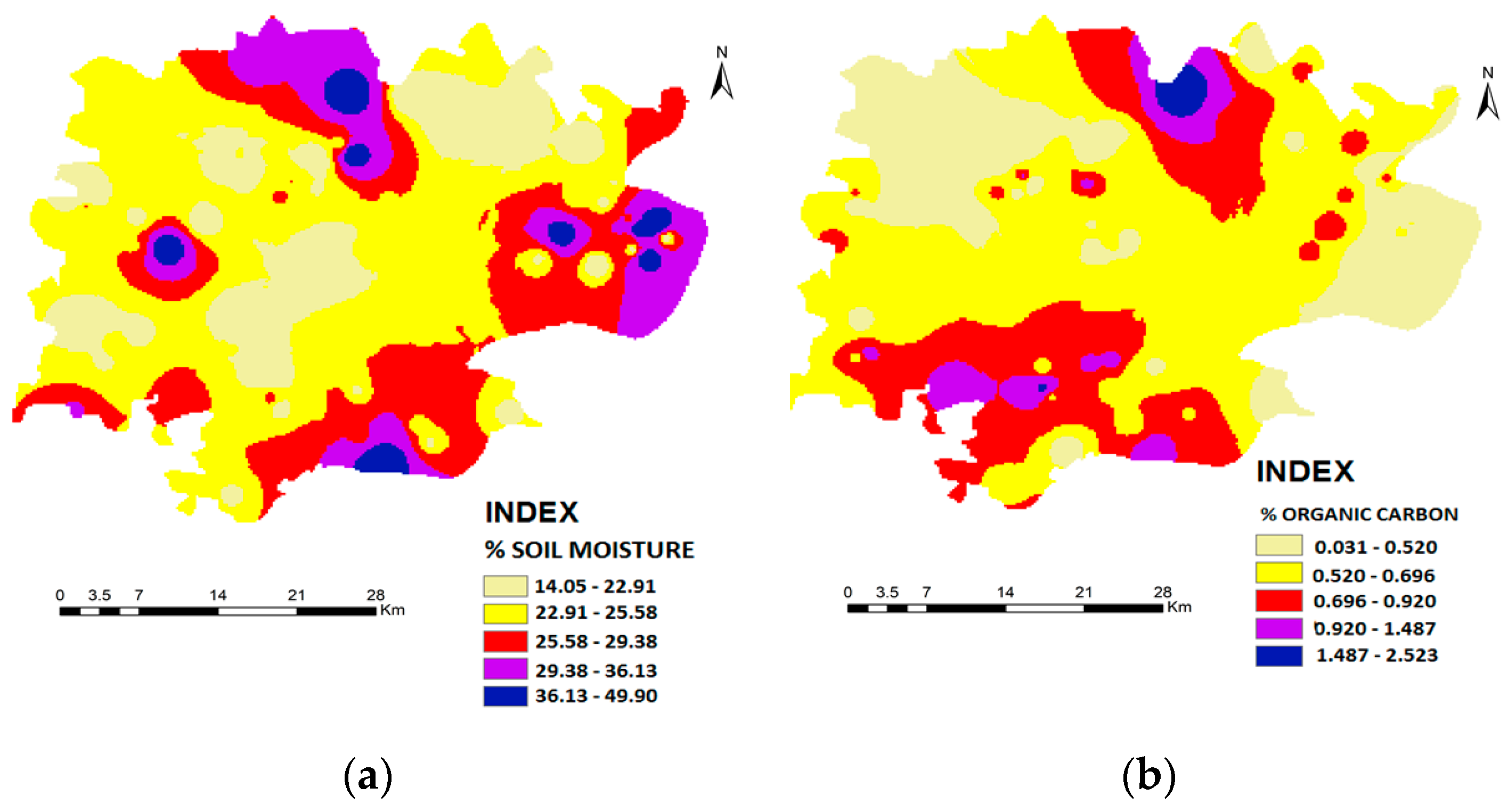
This study clearly demonstrated that the investigation of soil moisture distribution using GIS spatial interpolation techniques is an integral part of understanding the relationships between soil characteristics. Soil moisture is important not only to agriculture but also for hydrology and climatology. Remote sensing devices, such as satellite radiometers, are useful tools to obtain soil moisture information over a large region. However, effective ground truth calibrated data for satellite are lacking and this study fills this gap in providing values for soil moisture at local spatial level. Soil moisture distribution over the study area shows that higher elevation has lower soil moisture content and vice versa and its spatial distribution is not uniform over space and time. Even organic carbon profile has not certain pattern of distribution but in general, it is low in areas of vegetation cover and high in urban regions. The performance of spatial interpolation techniques depends on several parameters such as sample size, sampling design, sample spatial distribution, data (density and variation), surface type, data quality, input data uncertainty, poor choice or implementation techniques. Further data quality depends upon the distribution, accuracy, variance and range and spatial correlation for its performance. In this study, not all these mentioned parameters were incorporated individually due to constraints.
The study of spatial interpolation of soil moisture based on ground measurement data of soil moisture revealed that kriging with external (KED) is performing better than ordinary kriging (OK), inverse distance weighting (IDW) and Spline methods in terms of model accuracy and performance using cross validation techniques. KED is performing well over OK when secondary variable of organic carbon was added. This study can be extended in future, incorporating many parameters like soil texture, NDVI (Normalized Difference Vegetation Index), LST (Land Surface Temperature), bulk density and can also be calibrated by satellite data of soil moisture. This study can also lead a way for spatial analysts to see which method can perform well while adding more parameters and what will be the threshold.
