Article

Improving the Hydro-Morpho Dynamics of A River Confluence by Using Vanes

1
Department of Civil Engineering, Faculty of Engineering, Universiti Putra Malaysia, UPM Serdang 43400, Selangor, Malaysia
2
Centre for the Restoration of the Iraq Marshlands and Wetlands (CRIMW), Ministry of Water Resources, Baghdad 10065, Iraq
3
Water Resources Engineering, Faculty of Engineering, University of Baghdad, Baghdad 10071, Iraq
4
Hydraulic Research Laboratory, Hokkaido University, Sapporo 060-0817, Japan
*
Author to whom correspondence should be addressed.
Resources 2019, 8(1), 9; https://doi.org/10.3390/resources8010009
Submission received: 2 November 2018 / Revised: 12 December 2018 / Accepted: 24 December 2018 / Published: 1 January 2019

Abstract

:
Controlling the flow and bed morphology in a river confluence is important in training and navigation works. The flow in river confluence is highly complex due to crucial and rapid changes associated with flow dynamics, sediment transport, and geomorphology. The flow in Malaysia’s rivers has many confluence junctions in natural drains of catchment areas. The confluence between Kurau and Ara Rivers, in Perak, Malaysia, is selected to investigate the scour hole that usually forms in the erosion zone and the bar that forms in the deposition zone. A 2D numerical model is used in simulating hydro-morpho dynamics in the rivers confluence to mitigate the erosion and deposition zones by adopting vanes as control structures. Simulation results suggest that the most effective location, dimension, and angle of vanes can be decided based on their performance in scouring and deposition zones. The distribution velocity and flow vectors can help in deciding the location of the vanes.

1. Introduction

River confluence is important component of fluvial systems. Confluence results from the conjunction of separate flowing rivers, and this phenomenon produces a complex hydro-morpho dynamic environment [1]. Rapid changes occur in the fluid and sediment transport mechanism, causing a complex phenomenon of hydro-morphological dynamics in the confluence and affect the main river. The main river attempts to accommodate the water and sediment inflow supplied by two rivers. Given that confluences exist everywhere, the features of natural drains are vital in regulating the longitudinal distribution of flow and sediment [2,3,4,5]. Research on confluence dynamics is a relatively recent undertaking, and the phenomenon has been studied experimentally in the laboratory, wherein several features have been identified to study the mechanism of flow patterns and bed formation. In studying the hydraulics of a confluence, the plan form angle, discharge ratio, and momentum flux ratio are considered the major controlling factors [6,7,8,9,10,11,12,13]. Several studies [14,15,16,17,18,19,20,21] conducted field investigations of natural stream confluences to assess the relevance of experimental and numerical models for flow composition and morphology under natural conditions. Studies on confluences, including the development of theoretical frameworks, have integrated experimental or field research with numerical modeling [22,23,24,25,26]. A few studies on natural river confluences focused on the combination of flow and sediment transport [1,5,27]. Most experimental and numerical studies on river confluences confirmed that erosion and deposition zones form at the confluence site. The erosion zone involves a morphological process that usually occurs at the beds and outer banks of the river confluence and is known as the scouring hole, which is caused by high velocities. The deposition zone usually occurs at the inner banks (opposite to the location of erosion) and recognized as point bars or islands caused by sediment deposition due to low velocities. Scouring and sedimentation zones are the major morphological features of river confluences. The scour hole is associated with sediment transport caused by increased flow turbulence and velocity intensities at the confluence [3,17,28]. By contrast, deposition can be recognized clearly in the separation zone created under low pressure and flow recirculation. The separation zone in confluences exerts a direct influence on the flow dynamics and morphological features [29,30].
The erosion and deposition issues are considered as a main critical point in river confluences. The associated problems can be summarized as follows. The erosion process disturbs the environment of the river ecosystem, water quality, water consumption suitability for humans, and the industry [31,32]. Sediment accumulation results in reduced river capacity and considerable changes in a river’s hydro-morpho dynamic [33,34,35], especially in river confluences. Reduced river capacity and discharges from tributaries under heavy rainfall lead to an increase in the possibility of flood risks [36]. Most studies on river confluences were conducted on laboratory-scale models with mobile beds and rigid boundaries. The scale effects add to the complexity of the problem, and related research has primarily focused on parametric studies for predicting or simulating scouring and deposition zones. A few studies have been conducted on controlling and managing these morphological features, especially by introducing obstacles as a control structure.
An early study on controlling scouring and deposition zones by using a set of submerged vanes in 90° flume confluence adopted a typical vane layout for enhancing the navigation of river confluences [37]. The layout was designed to decrease the velocity in the erosion zone (scouring zone) which consequently led to decrease water depth, this process occurred as a result of redirecting the flow by vane layout from the erosion zone toward deposition zone. Increasing the flow in the deposition zone lead to an increase in the velocity, thereby leading to the removal of a large portion of sediment from the bar that formed in the deposition zone. Two recent studies were conducted on a laboratory scale with 60° and 90° confluences [38,39], in which a set of vanes and piles were proposed to control bed erosion. The results of these studies show that the maximum percentage of reducing the scour depth is 55% and 43% with 90° and 60° confluences, respectively, through the use of a set of piles; the reduction is less than 10% from the above percentage when a set of vanes is used. Furthermore, the studies placed the vanes at angles of 15°, 30°, and 60° and found that increasing the vane angle by more than 30° leads to increased scour depth.
The mitigation of scouring and deposition zones is considered an acute research gap that requires further investigation. This study selected a natural river confluence in a tropical region (confluence of Kurau and Ara Rivers in Perak, Malaysia). The flow in Malaysia’s rivers has many natural confluences, and at these confluences, consistent cross-section changes occur due to sediment movement. Thus, river capacity is reduced, and flood levels are increased because of sediment accumulation [33,34,35,40]. Human activity in the catchment of the selected area has increased, especially in changes in land use from 2004 to 2015 [41]. These changes have led to increased river sand mining, which has resulted in changes in river hydrology and increased sediment load along the river; it has also affected the water supply for irrigation and municipalities and flood control schemes.
The Mflow_02 solver (operated by the International River Interface Cooperative (iRIC), Hokkaido, Japan) was used in the current study to simulate the hydro-morpho dynamics of Kurau and Ara river confluence in Malaysia. The simulation included identifying the locations of scouring and deposition zones and investigating the effectiveness of introducing vanes. Vanes have been proposed as control structures to mitigate scouring and deposition zones and thus improve the hydro-morphological characteristics of the river confluence site. An obstacle is generally used to improve the navigation of a river through redirect the distribution of the flow and enhance the alignment of the river and bank erosion protection. The hydraulic performance of the obstacle depends mainly on its location, angles, dimensions, and morphological conditions [42,43,44]. For this reason, no specific criteria are used for designing an obstacle in a river system. Thus, in this study, an obstacle (i.e., a vane) was used as a control structure in the selected river confluence. Physical or numerical simulation is required to optimize the design of the vane. However, using physical models entails several limitations, such as high cost, steady flow, and scale effect. By contrast, numerical models are low-cost and can be used efficiently for unsteady mobile bed conditions. The significance of this study is attributed to the simulation of various scenarios for controlling scour and deposition zones by using vanes and recommended the best solution that provides minimum scouring and deposition zones and enhances river flow dynamics.

2. Materials and Methods

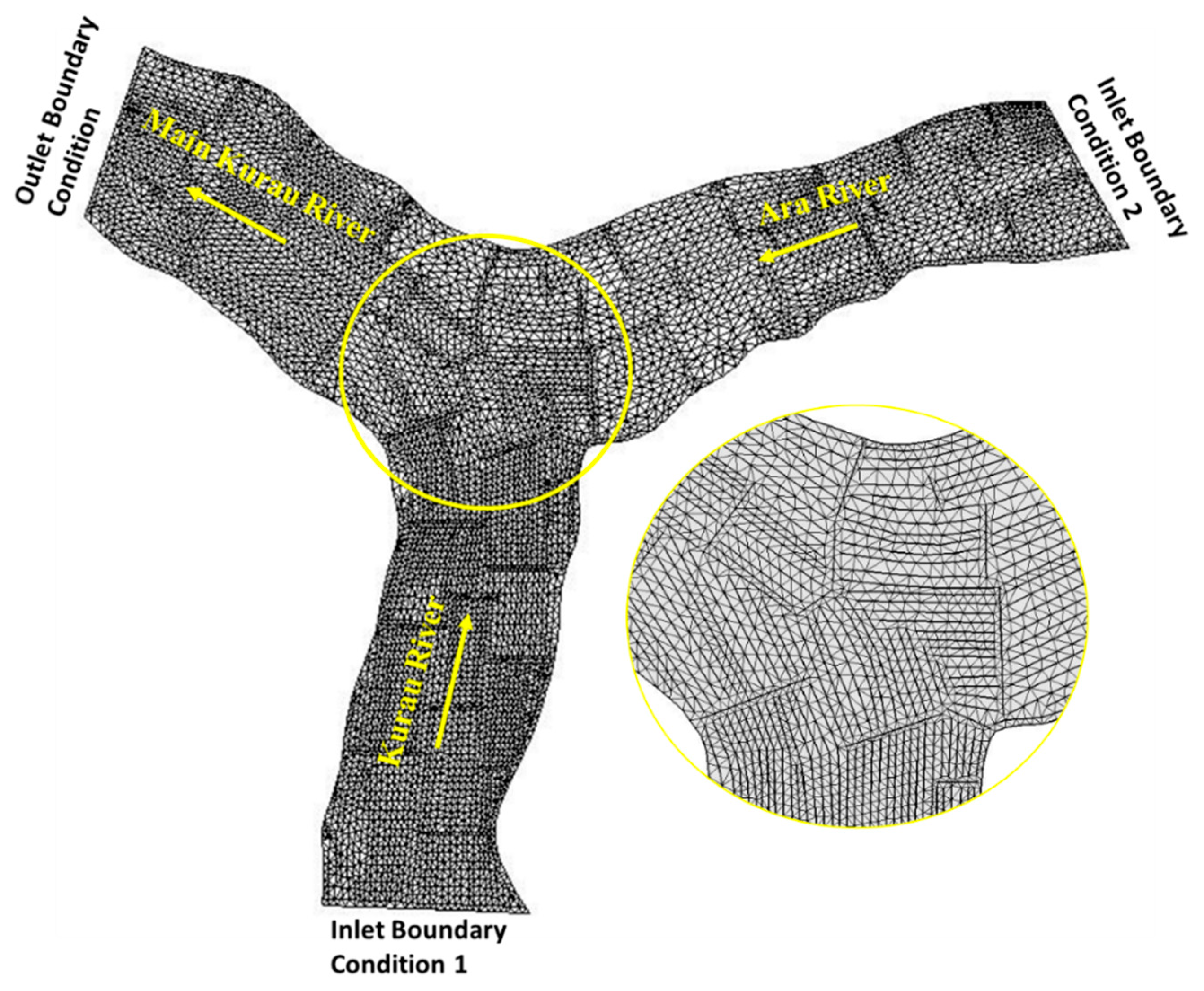
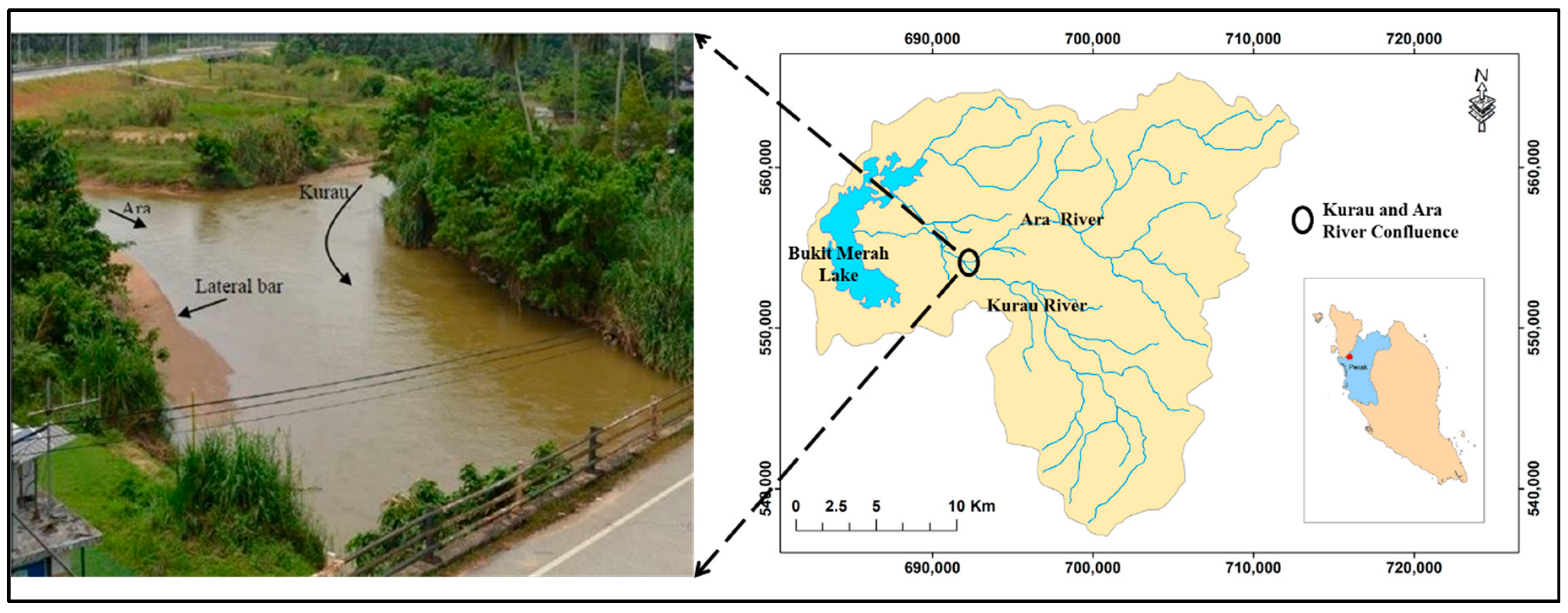
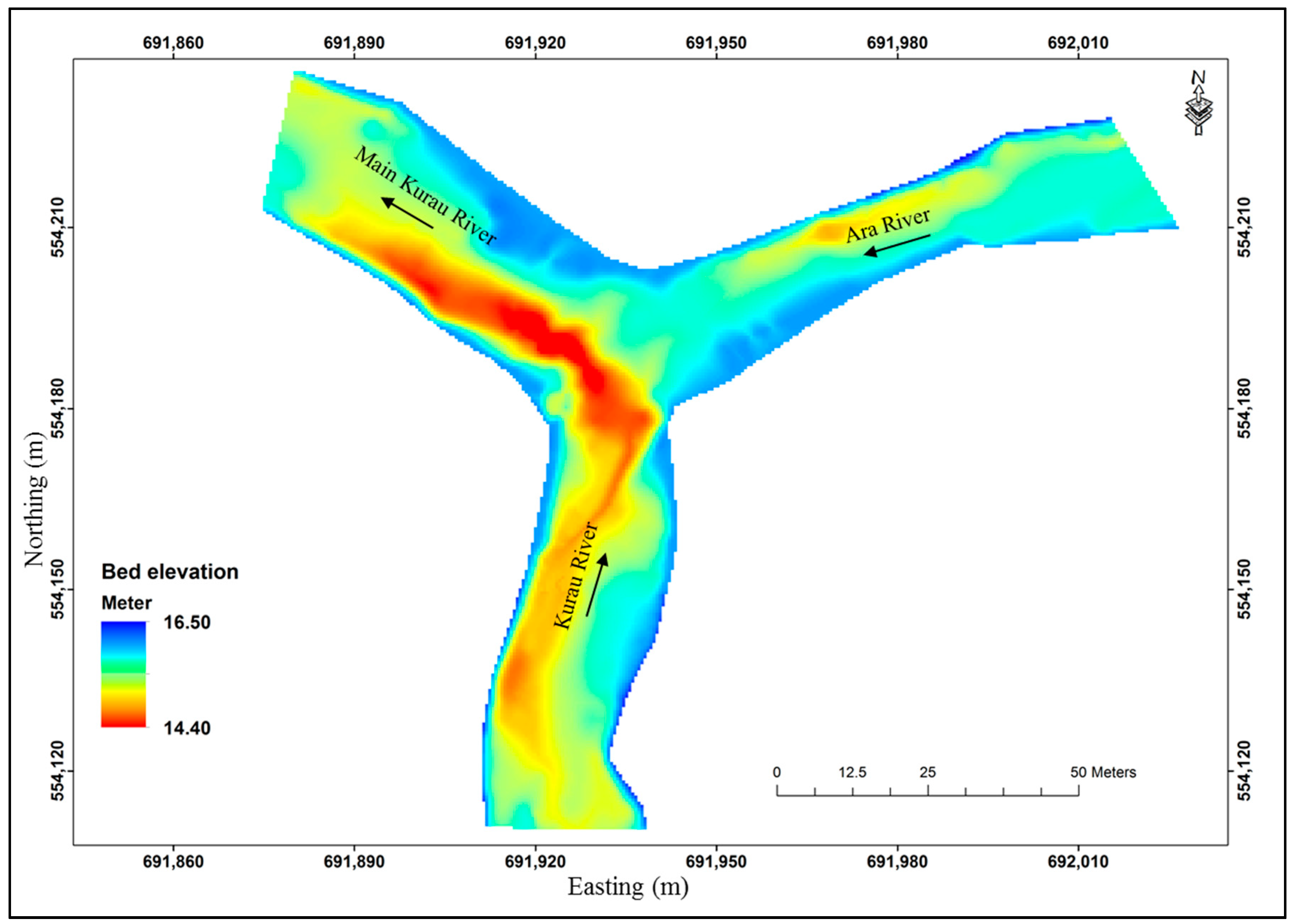
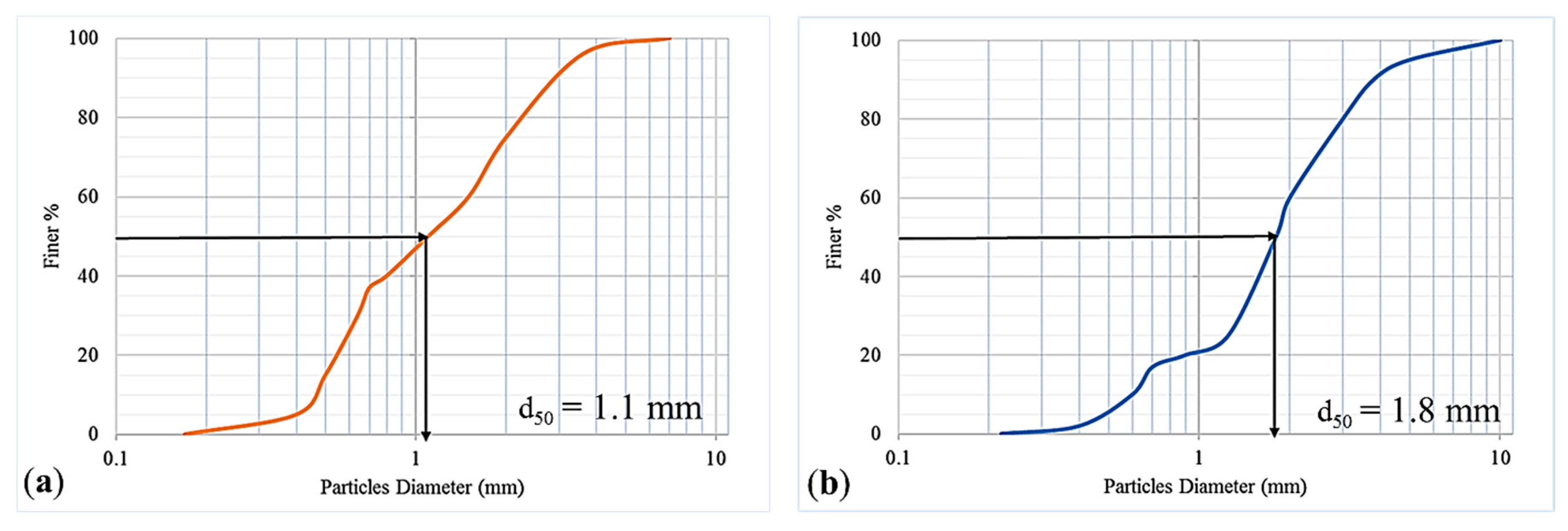
2.1. Study Area and Data Acquisition

The main catchment area of Bukit Merah Lake is formed by the meeting of two sub-basins of rivers Kurau and Ara. The confluence of these rivers is located at Pondok Tanjung approximately 7 km upstream of Bukit Merah Lake and northwest of Perak State, Malaysia (Figure 1). The rivers start from the mountain area where the averaged slope is 12.5%, and terrains at the mid and lower reaches are undulating with an average slope of 5%. The lower reach is exposed to floods due to its flat and wide floodplains [45]. The confluence of Kurau and Ara Rivers has different widths and bed levels. The average width of Kurau River is approximately 23 m, whereas that of Ara River is 28 m. The bed levels of Ara River are approximately 0.45 m higher than the bed levels of Kurau River and these rivers meet at an angle of 135°.
Data on hydro-morpho dynamics of the Kurau and Ara river confluence were obtained from Sirdari [46], and included information on discharges, water levels, velocities, and transect geometry. Sediment measurements were conducted on a series of cross sections at the confluence in April and September 2012. Data were obtained from hydrodynamic measurements and bathymetric surveys by using a SonTek River Surveyor device S5. Figure 2 shows that the digital elevation model (DEM) resulted from measuring 40 cross sections at the Kurau–Ara confluence, and the details of these cross sections have been stated in [46], in which the primary results of the bathymetry survey confirmed the hydro-morpho dynamic features that were reported in literature.
The average median particle ( d 50 ) of the bed material for the Kurau and Ara river confluence was 1.1 mm (Figure 3a), whereas that for the scouring zones located near the left bank of main Kurau was 1.8 mm (Figure 3b). The particle size distribution curves are presented as an average curve obtained from measuring approximately seven points from the left to the right bank at different cross sections in the selected river confluence and under different flow events; further details were provided by [46]. A dataset that included discharge, velocity, water level, cross section, and bathymetry survey was created on 09/04/2012. The set was used to build and calibrate the model, and seven other data sets were used for model validation. The discharge changes daily because the area is located in a tropical region and results in different rain events in the catchment.

2.2. Critical Velocity of Sediment Inception Motion

The critical shear velocity ( U c * ) of the bed material in this study was determined by using Shield’s diagram. The dimensionless shear stress ( T * ) expressed in Equation (1) was obtained from the diagram. Critical shear velocity was calculated from Equation (2).
T * = τ c ( γ s γ ) d 50
U c * = τ c ρ
where τ c : critical shear stress of the bed material; γ s : specific weight of the bed material; γ : specific weight of water; ρ : water density; d 50 : median particle diameter.
Using Shield’s diagram and applying Equations (1) and (2) showed that the values of critical shear velocity for the bed material with a median particle diameter ( d 50 ) between 1.1 and 1.8 mm varied between 0.025 and 0.034 m/s for the selected river confluence.
For moveable bed and sediment transport, knowing the threshold point of sediment particles in motion is important, and most existent studies represented the threshold point of sediment particles in terms of critical mean velocity, namely, V c . Many methods are available for estimating the critical mean velocity, and one of the most common ones is the Simons and Şentürk method, which is shown in Equation (3) [47,48].
This equation is frequently adopted to compute the critical mean velocity, and the values are between 0.56 and 0.9 m/s with low and high water depths ( y ). The value of critical velocity is a function of water depth ( y ), in which the median particle diameter ( d 50 ) is known and the other variables are kept constant for the selected river confluence.
V c = 1.58   ( ρ s ρ 1 ) g d 50 ( y d 50 ) 0.167
where ρ s : sediment density.

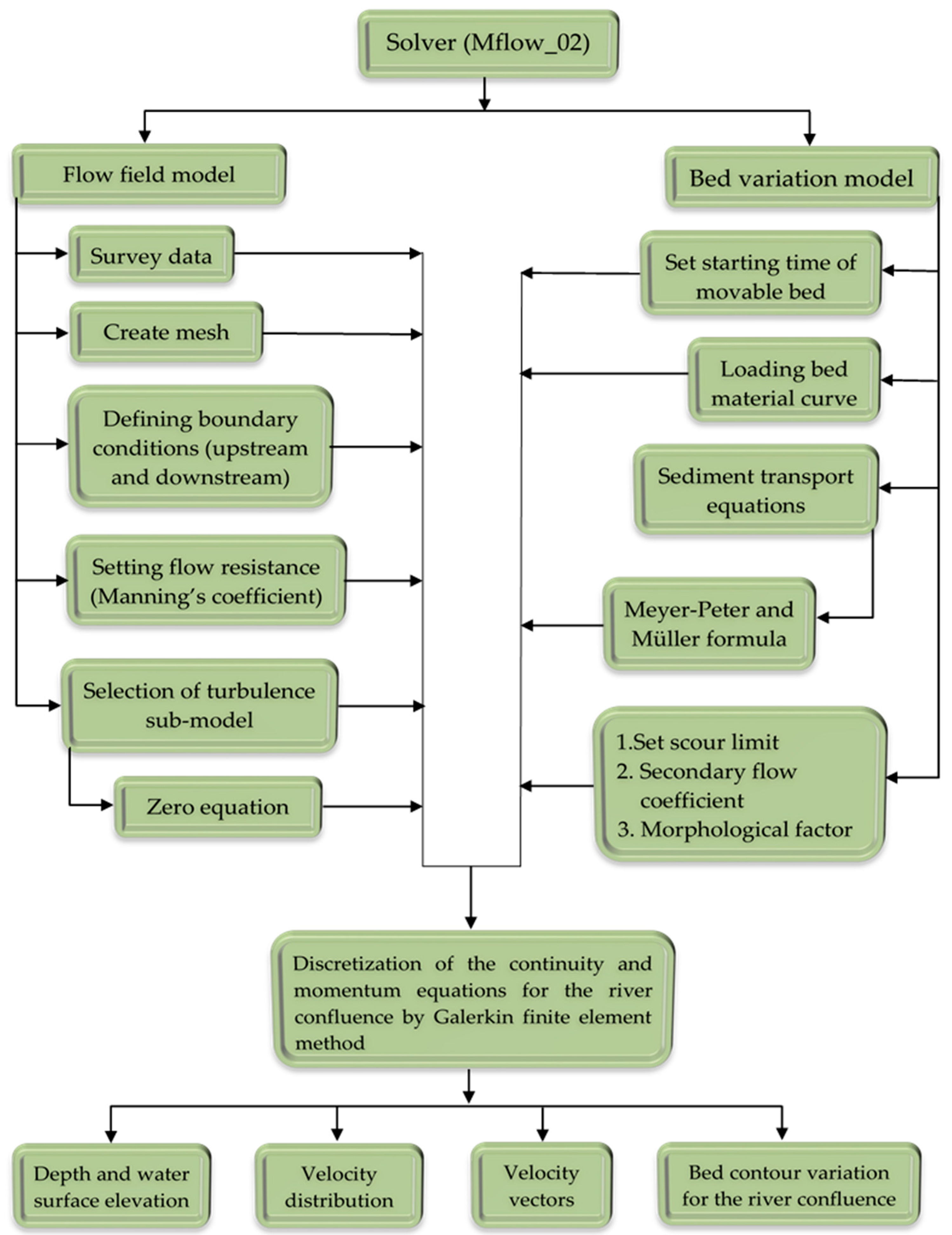
2.3. Solver Background, Structure, and Characteristics

In this study, the solver Mflow_02 was used as a tool to simulate unsteady flow in the selected confluence of Kurau and Ara Rivers Malaysia. The original version of Mflow_02 was based on the program developed by Tomitokoro et al. [49], and recently the program of the solver was improved by iRIC [50]. The improvement included adding certain functions, such as moving boundary model and riverbed variation calculation. Thus, the program can calculate 2D plane unsteady flow and riverbed variation by using unstructured meshes of the finite element method in an orthogonal coordinate system (Cartesian coordinate system). Subsequent development resulted in the model being able to reproduce exactly the structure and shape of complicated landforms, particularly in distributaries and confluences. Thus, the Mflow_02 solver was used in this work to simulate the morphological dynamics of the selected confluence of Kurau and Ara Rivers in Perak State, Malaysia, including the proposed solutions for controlling the scouring and deposition zones. Two main models—namely, flow field and riverbed variation models—are embedded in the Mflow_02 solver. These models have many sub-models that can help achieve a wide range of calculations.

2.3.1. Flow Field Model

The characteristics of the flow field model are as follows:
  • A Galerkin finite element sub-model (a type of weighted residual method) is used to discretize continuity and momentum equations.
  • Open boundary conditions (upstream and downstream boundaries, etc.), enable the setting up of various conditions, such as time series of flow discharge, time series of water level, and water level discharge.
  • The friction of the river bed can be set by using the Manning roughness coefficient. This coefficient can be represented in the model as a polygon for the entire area or for each element (cell), thus providing spatial distribution of roughness.
  • Three sub-models are available for computing the turbulence field (flows with large and small eddies). These are the zero equation sub-model, simple k-ε, and direct input of kinematic eddy viscosity. In this study, the zero equation sub-model was selected because of its stability in calculating large and small eddies. The kinematic eddy viscosity, υ, is expressed by using the von Kàrmàn coefficient with k (0.40).
    v = k 6   u *   y
    where u * : bottom friction velocity.
This formula is called the zero equation sub-model for turbulence statistics without a transport equation. In flow fields wherein water depth and roughness are changed gradually in the cross sections of river confluences, the kinematic eddy viscosity in horizontal and vertical directions is assumed to be in the same order.
5.
Other effects, such as the effect of wind on the water surface and of vegetation on flow, are available in this solver but were disregarded in this study.

2.3.2. Riverbed Variation Model

The characteristics of riverbed variation are as follows:
  • The riverbed variation associated with the flow field model is calculated. This model can calculate the flow field only or together with riverbed variation.
  • The riverbed material can be selected from uniform and mixed grain diameters. If a mixed grain diameter is selected, then a variation in grain distribution can be assumed for deep directions and multiple layers.
  • Three methods for calculating the total bed load q b of depth-averaged flow velocity are available in the Mflow_02 solver, and these are the Meyer-Peter and Müller formula [51], Ashida and Michiue formula [52], and Engelund-Hansen formula [53]. In this study, the Meyer-Peter and Müller formula was adopted for computing the total bed load.
q b = 8   ( σ ρ 1 )   g   d 50 3 ( τ * τ * c ) 1.5
where σ : gravel density; τ * c : critical tractive force (calculated by the Iwagaki formula, [54]); τ * : calculated by Kishi and Kuroki in the formula below
U ¯ u * = 7.66   ( y 2 d 50 ) 1 / 6   ( τ * τ * ) 2 / 3 y 2 d 50 < 500 ( 6 ) 11.59   ( y 2 d 50 ) 1 / 10   ( τ * τ * ) 3 / 5 y 2 d 50 500 ( 7 )
where U ¯ : vertical average flow velocity in the flow direction.
The total sediment discharge set by the Meyer-Peter and Müller formula is converted to the normal direction (n) and tangential direction (s) of the streamline, in consideration of the effect of secondary flow and riverbed slope, which is caused by streamline curvature of depth-averaged flow velocity.
q s =   q b   ( ν b V b   τ * c μ s   μ k   τ * z s )
q n =   q b   ( u b V b   τ * c μ s   μ k   τ * z n )
where q s : (s) direction component of sediment discharge near the riverbed; q n : (n) direction component of sediment discharge near the riverbed; V b : absolute value of velocity near the riverbed; ν b : (s) direction component of flow velocity near the riverbed; u b : (n) direction component of flow velocity near the riverbed; μ s : static friction factor; μ k : kinetic friction factor; z : height of the riverbed.
Further explanations the above equation can be found in Watanabe et al. [55] and Hasegawa [56].
4.
The scour limit of the riverbed, secondary flow coefficient, and morphological factor can be set accordingly.
Figure 4 shows additional details on the solver’s application.

2.4. Model Implementation and Boundary Conditions

The Mflow_02 model was used to assess morphological changes in the river confluence. The initial input data were imported from a bathymetry survey for the confluence of Kurau and Ara Rivers. A fine unstructured grid consisting of 6136 nodes was created by drawing many lines until good performance was achieved (Figure 5). A finer grid resolution provides more accurate results, but it needs a small time step (Δt). Time step has a direct relationship with the dimension of the grid ( d l ) and velocity ( V ), which can be expressed as Δ t d l V . In the current model, different time steps were attempted until the hydrodynamic simulation operated smoothly with a time step of 0.01s. The second input data comprised the curves of the grain size distribution of the bed material. The measured data indicated that the average median particles of the rivers were approximately 1.1 mm for the normal depth and 1.8 mm for the deep hole (scouring).
The third input data contained the flow rate at the upstream and the water level at the downstream. A flow rate of 6.33 m3/s was set in inlet boundary condition 1 upstream of Kurau River, whereas a flow rate of 6.43 m3/s was set in inlet boundary condition 2 upstream of Ara River. A water level of 16.26 a.m.s.l was set in the outlet boundary condition that is located downstream of the main Kurau River. Among the turbulence models, a zero-equation model was adopted, and movable bed computation with a starting time of 800 s was set up to provide stability to the flow regime operation first and then sediment transport and bed deformation afterward. For sediment transport computation, Mflow_02 uses Ashida and Michiue [52], Meyer-Peter and Müller [51], and Engelund-Hansen [53] equations to compute the total bed load transport. In this study, the Meyer-Peter and Müller equation was selected to conduct sediment transport computation because the equation provides reasonable results for simulated bed elevations. The accuracy of the simulated bed elevations was demonstrated in both models’ calibration and validation results. Other settings related to riverbed morphology and sediment transport were as follows: the scour limit of the riverbed in which in the selected river confluence has no limit for scouring was set in the model, the secondary flow coefficient was set to 7 (based on the Engelund model [53]), and the morphological factor (the ratio of bed deformation to flow) was set to 1. The above setting was considered for a real simulation, in which an increase in one of these values leads to an increase in the bed deformation of the river confluence.

2.5. Hydraulic Performance of the Proposed Vanes Used in The River Confluence

Many types of obstacles are used in the riverine system to manage and control the training of the rivers. Spur dykes, vanes, groynes, and weirs are among the obstacles used by U.S. Army Corps of Engineers [41]. In this study, vanes were used as obstacles to assess the hydro-morpho dynamics of the natural rivers at confluence. This type of structure was introduced in the model by creating a polygon that was excluded throughout mesh computing and regarded by the model as a non-erodible bed material [50]. The impact of the following three scenarios on the flow in a confluence of Kurau and Ara Rivers was clearly shown in the computation of riverbed variation and velocity distribution with the development, appearance, and movement of the sandbar.
  • Single row of the vanes with a length of 1 m and a spacing of 6 m between vanes
  • Single row of the vanes with a length of 2 m and a spacing of 5 m between vanes
  • Single vane a length of with 10 m

2.6. Statistical Indices

Four statistical indices were used to assess the accuracy of the prediction of the Mflow_02 model, and these were mean absolute deviation (MAD), mean square error (MSE), root mean square error (RMSE), and mean absolute percentage error (MAPE). The criterion for using these methods is to determine the accuracy of the simulation, in which a low statistical value between measured and predicted values indicates high accuracy of simulation performance. These methods can be described by the equations
MAD = n = 1 n | M S | n
MSE = n = 1 n ( M S ) 2 n
RMSE = n = 1 n ( M S ) 2 n
MAPE = n = 1 n | M S M | n 100 %
where n: amount of data used; M: measured value; S: simulated value.

3. Results and Discussion

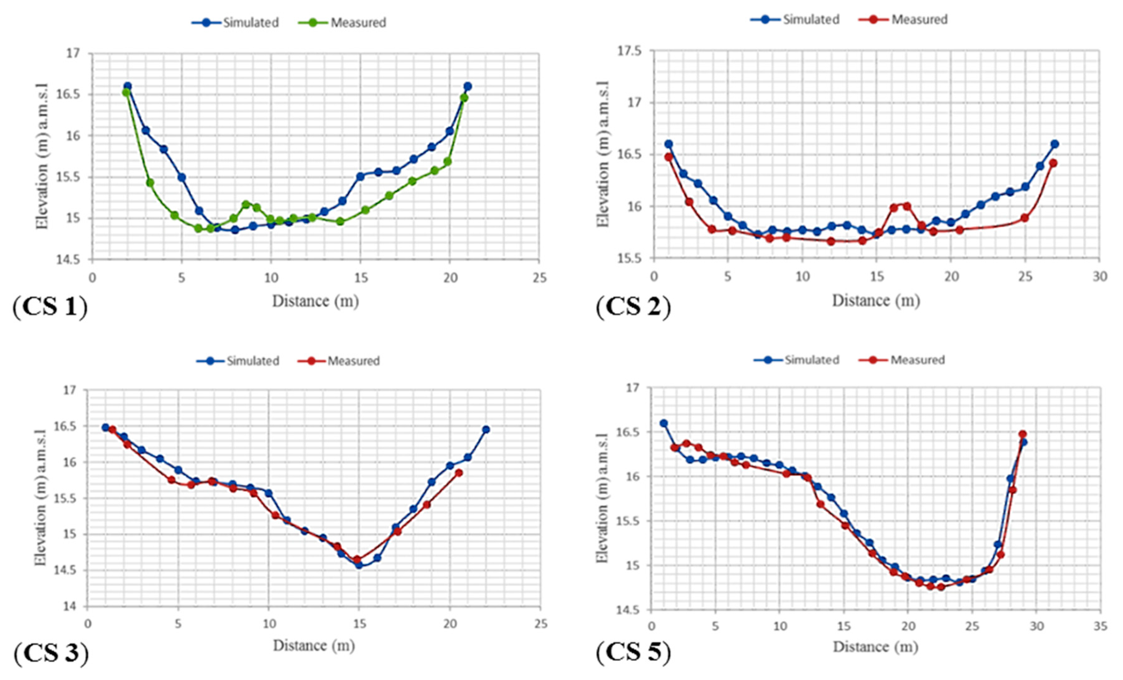
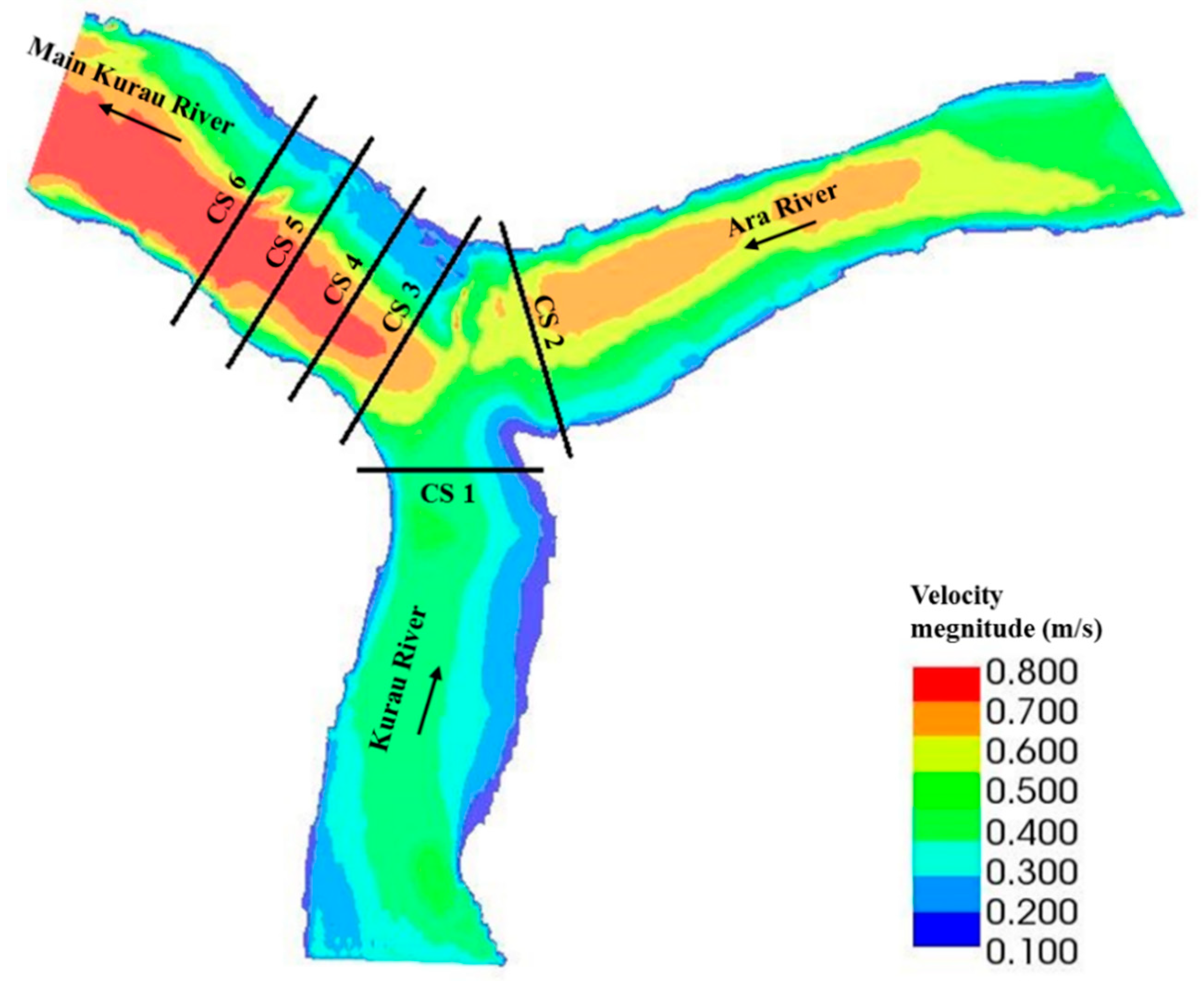
3.1. Model Calibration

The model was calibrated with Manning’s roughness n = 0.063, in which the adopted value was calculated based on field measures of two studies [46,57], node number, time step, and turbulence model until good agreement was found between model prediction and measured data on flow velocity, water surface elevation, and bed elevation. The results of velocity magnitude for running the model for 24 h (the simulation time of the model calibration) are shown in Figure 6, and the average values of the simulated velocities along the cross sections at different times (1, 2, 3, 6, 12, 18, and 24 h) are shown in Figure 7. A summary of the simulated and measured velocities is shown in Table 1. The velocity at different times confirmed the stability of running the software and how much the velocity changed during the 24 h within the same boundary conditions.
Four statistical indices were used to assess the accuracy of the measured and predicted averaged flow velocities of model calibration. These indices were MAD in Equation (10), MSE in Equation (11), RMSE in Equation (10), and MAPE in Equation (10). The results of the statistical indices are shown in Table 2. The error values differed because they depend on their concepts. The maximum error was associated with MAPE and approximately 9%. In general, MAPE provided values higher than those of other methods because it represents the percentage of the difference between measured and predicted values divided by measured values. However, the measured and simulated average velocities matched well.
The simulation of water surface elevation is shown in Figure 8. The simulated and measured water surface elevations at different locations had minimum errors because the boundary condition at the outlet was time-varying elevation. The values of MAD, MSE, RMSE, and MAPE between measured and simulated results were 0.024 m, 0.001 m, 0.028 m, and 0.144%, respectively, and the error values of the errors are shown in Table 3.
To ensure the accuracy of the morpho-dynamics simulation, calibration was performed by comparing the simulated and measured bed elevations. Figure 9 shows the depth simulation with the location of four cross sections at the confluence of Kurau and Ara Rivers. These sections were used to demonstrate the difference between measured and simulated bed elevations (Figure 10). The calibration process was based on the model output obtained after running the model continuously for 24 h. The comparisons showed good agreements between simulated and measured bed elevations and confirmed the accuracy of the model output.

3.2. Model Validation

The model was validated with different data sets of the confluence of Kura and Ara Rivers for the period of seven days in order to increase and display the accuracy of the simulation for the selected study area. A comparison was performed between simulated and measured water levels, average depths, average velocities, and bed elevations. Data for the unsteady flow in the upstream of Kurau and Ara Rivers and the water level at the downstream of the main Kurau River are shown in Table 4. The model’s running time was approximately eight days for the period of seven days’ data with 6136 nodes and 0.01s time step.
To demonstrate the accuracy of model prediction, the simulation results on the second and fourth days (with discharges of 15 and 43 m3/s, respectively) were compared with measured data on water level, average flow depth, average velocity, and bed elevation. The model output showed that the simulation of water levels was highly accurate according to the values of the four statistical indices Table 5 and Table 6. The values of MAD, MSE, RMSE, and MAPE were determined using the predicted and measured data. These values were 0.032 m, 0.001 m, 0.034 m, and 0.198%, respectively, for a discharge of 15 m3/s, whereas those for a discharge of 43 m3/s were 0.083 m, 0.008 m, 0.087 m, and 0.484%, respectively. The simulated average flow depth was within the observed range, and the values of the statistical indices were 0.04 m, 0.002 m, 0.044 m, and 4.486% associated with a discharge value of 15 m3/s. By contrast, for the discharge value of 43 m3/s, MAD, MSE, RMSE, and MAPE were 0.075 m, 0.008 m, 0.087 m, and 4.707%, respectively.
The simulated average velocities were in agreement with the measured average velocities as shown in Table 7. Most of the simulated velocities in the Kurau River were lower than the measured velocities, and the maximum error was associated with high discharge. MAPE was 19.1%, whereas at low discharge, the MAPE was 10%. The errors refer to the uncertainty in the measured and predicted values. Papanicolaou et al. [58] reported that the typical acceptable errors in depth and velocity predictions are in the rang 25% and 35%. Pinto et al. [59] suggested accepting the under prediction in velocity because it results in fewer errors. The above range of errors is acceptable when compared with other simulated results [42,60].
With regard to the morphological validation, Mflow_02 showed the model’s capability to simulate morphological changes such as scouring, deposition, and movement of sediment transport, leading to changes in cross sections. The simulated and measured cross sections are shown in Figure 11 and Figure 12.
For the discharge of 15 m3/s, the simulated and measured bed elevations were in agreement, particularly in cross-sections 3 and 5. Reduced agreement was found in cross-sections 1 and 2. For the discharge of 43 m3/s, the highest agreement between the measured and simulated cross-sections were found in cross-sections 1 and 5, whereas the least agreement was found in cross-sections 2 and 3. The errors between measured and simulated elevations in the cross sections can be attributed to the spatial location of the collected data and to a complex river reach geometry. Papanicolaou et al. [61] related the sources of errors to computational errors from the numerical schemes used in solving the governing equations and to the truncation errors from discretization. In addition, data collection could be another source of errors. For example, the eddy viscosity models used in solving the governing hydrodynamic equations for turbulent flows had some degree of empiricism in their formulations.

3.3. Evaluation of Hydraulic Performance of the Proposed Vanes Used in the River Confluence

The simulation of the confluence bathymetry with and without vanes after the third day of the model run with the discharge of 43 m3/s was analyzed, because of its effect on the hydro-morpho dynamics. It was recognized in the confluence zone and marked as the change in flow depth, scouring zone, deposition zone, and velocities with its vectors. Six model runs with vanes were compared with running the model without vanes. The time of running each model was approximately eight days. The details and evaluation of these models can be summarized in the following three scenarios. Each scenario was implemented twice with vane angles of (15° and 30°) in the flow direction of Ara river.

3.3.1. First Scenario: Single Row of the Vanes with a Length of 1 m

The maximum scour zone that formed at the junction near the outer bank of the main Kurau River was caused by high flow from the Ara River that deviated the flow of the Kurau River toward the outer bank at the beginning of the main Kurau River. At this location, the velocity was increased, and current and eddies were created and considered the main cause for the maximum scour zone. At the opposite side near the inner bank of the main Kurau River, low velocity was found and considered the main reason for the deposition zone. A single row of vanes with 1 m length was introduced at the junction near the Ara River’s mouth to manage and reduce scouring and deposition zones. The length of a single vane was calculated based on water depth, which is equal to 0.3 of the flow depth [39]. The spacing between them was obtained by multiplying the flow depth by 2. These criteria were recommended by Odgaard and Wang [37] and Allahyonesi et al. [62]. In addition, the optimum angles of the vanes were taken as 15° and 30°. Optimum angles for vanes were recommended by Odgaard and Spoljaric [63], Barkdoll et al. [64] and Wuppukondur and Chandra [38,39]. Furthermore, they reported that scour depth increases with an increase in vane angle, and the minimum scour depth is at angles of 15° and 30°. Two models were operated by using the data on unsteady flow shown in Table 4. The model outputs with and without vanes were compared for a discharge of 43 m3/s. Figure 13 and Figure 14 show a comparison of water depth when vanes were introduced with angles of 15° and 30°, respectively, Figure 15 and Figure 16 show a comparison of velocity distribution and its vectors for vanes with angles of 15° and 30°, respectively. In this scenario, the simulation results of introducing inclined vanes show that not much change occurred in the maximum scour zone near the outer bank and in the flow depth near the inner bank (deposition zone) of the confluence. The impact of the inclination angle of the vanes was evident in the flow depth behind vanes, where the flow depth decreased when an angle of 15° was used. This result is attributed to fact that low velocities were created behind the vanes (Figure 13b), and this increased the potential of sediment deposition, as shown in Figure 13b.

3.3.2. Second Scenario: Single Row of Vanes with a Length of 2 m

In the second scenario, the simulation included introducing a single row of inclined vanes with 2 m length and a spacing of 5 m. The angles of inclination of the vanes were 15° and 30° with the flow direction of the Ara River. The simulation results included the impacts of inclination angles on flow depth, velocity, and velocity vectors, as shown in Figure 13c, Figure 14c, Figure 15c and Figure 16c. The angle of the vanes was a major factor in controlling the morphological change at the confluence of Kurau and Ara Rivers, where the flow depth decreased in the scour zone and the maximum scour zone was almost diminished, particularly when the vanes were introduced with an angle of 30°. The depth in the deposition zone increased in several parts of this zone, and increasing the flow depth in this zone is needed. In the case of vanes with an angle of 15°, the flow depth behind the vanes decreased, and point bars appeared especially in the locations of the first three vanes in the main Kurau River. These point bars were associated with low velocities behind the obstacles/vanes.

3.3.3. Third Scenario: Single Vane with a Length of 10 m

In this scenario, a single vane with a length of 10 m was introduced with angles of 15° and 30° in the same location of the vanes used in the first and second scenarios. The simulated flow depth, velocity, and velocity vectors are shown in Figure 13d, Figure 14d, Figure 15d and Figure 16d. The results showed that the maximum scour hole was diminished, and the deposition zone was maintained. The impact of the angles on flow depth and velocity distribution was obvious. The flow depth at the tip of the vane with an angle of 15° was much larger than that with an angle of 30°. Furthermore, the velocity behind the vane at an angle of 15° was lower than that with an angle of 30°. The function of the vane was to divert the direction of the flow toward the zone with low pressure and velocity (flow separation zone), and it also maintained the potential of sediment movement and deposition. The velocity in this zone increased from 0.5 to 0.7 m/s, and this value exceeded the value of critical mean velocity at this zone, which is 0.56 m/s. The movement of bed sediment particles occurred when the mean velocity increased and exceeded the critical mean velocity of the sediment. The increment in velocity led to increased bottom friction velocity ( u * ), and this value exerted a direct effect on the calculation of riverbed shear stress ( τ * ). Increasing τ * would result in increased sediment movement. Furthermore, the strength of local currents and eddies formed behind the location of the vane at an angle of 15° was weaker than that formed behind the location of the vane at an angle of 30°. Therefore, the sediment deposition in this location was significant. This scenario shows better performance in managing hydro-morpho dynamics compared with the other tested scenarios.
The length, number, and spacing of the first scenario were calculated following Odgaard and Wang [37], and the results obtained did not yield significant solutions to the hydro-morpho dynamics of the selected river confluence. In the second scenario, the length of the vanes was doubled to increase efficiency. The increase in vane length only worked with an angle of 30°. Owing to the lack of specific criteria on using vanes in a river confluence, the results from the first and second scenarios showed that the number of vanes produced a non-uniform velocity distribution, especially near the vanes. Therefore, a single vane was proposed to enhance hydro-morpho dynamics in a river confluence. The results obtained from introducing a single vane provided the best solution for maintaining hydro-morpho dynamics and enhanced the navigation of the confluence of Kurau and Ara Rivers.

5. Conclusions

The control of flow in river confluences is complex due to different hydro-morpho dynamic features that arise in these turbulence zones. A 2D numerical model was used in this work to simulate the hydro-morpho dynamics of the natural confluence of Kurau and Ara Rivers in Perak, Malaysia. The numerical model was calibrated and validated using field data. Vanes were proposed to control the scouring and deposition zones that usually exist in natural river confluences. Furthermore, the Mflow_02 model was applied to simulate the morphological changes for three scenarios with different vane arrangements. The results showed that increasing the vane length with an angle of 15° did not produce any significant change in the reduction of scouring and deposition zones. By contrast, the vanes introduced at an angle of 30° showed good performance in controlling the scouring and deposition zones. The flow interaction with vanes placed at an angle of 30° was much better than that with an angle of 15° due to low currents, eddies, and sediment deposited behind vanes. The results also showed that the number of vanes produced a non-uniform velocity distribution, especially behind the vanes, thereby leading to the appearance of point bars. The best results in terms of reducing the scouring and deposition zones were associated with introducing a single vane compared with the other tested scenarios. Future studies may apply the proposed mitigation process in another study area to validate the performance of introducing a single vane. Furthermore, other shapes of a single vane can be tested in the study area. In summary, this study addressed the applicability of using a 2D numerical model in a complex riverine system for predicting and managing hydro-morpho dynamic changes with and without vanes as training structures in a dynamic river confluence.

Author Contributions

B.Y. and H.L.A. conceptualization the overall idea of this research. T.A.M. and H.L.A. designed overall the methodology; Y.S. provided the software with training; H.L.A. carried out the computer simulations; H.L.A. wrote the paper; M.S.A.R. and B.M.R. review and editing the paper.

Funding

This research received no external funding and the APC was funded by Universiti Putra Malaysia.

Acknowledgments

We express our sincere thanks to Dato, Aminuddin Ab. Ghani, Deputy Director at River Engineering and Urban Drainage Research Center (REDAC), Universiti Sains Malaysia, for permitting reuse of the data.

Conflicts of Interest

The authors declare no conflict of interest.

References

  1. Riley, J.D.; Rhoads, B.L.; Parsons, D.R.; Johnson, K.K. Influence of junction angle on three-dimensional flow structure and bed morphology at confluent meander bends during different hydrological conditions. Earth Surf. Process. Landforms 2014, 40, 252–271. [Google Scholar] [CrossRef]
  2. Ashmore, P.; Parker, G. Confluence scour in coarse braided streams. Water Resour. Res. 1983, 19, 392–402. [Google Scholar] [CrossRef] [Green Version]
  3. Guillén-Ludeña, S.; Franca, M.J.; Cardoso, A.H.; Schleiss, A.J. Evolution of the hydromorphodynamics of mountain rivesr confluences for varying discharge ratios and junction angles. Geomorphology 2016, 255, 1–15. [Google Scholar] [CrossRef]
  4. Rhoads, B.L. Mean structure of transport-effective flows at an asymmetrical confluence when the main stream is dominant. In Coherent Flow Structures in Open Channels; Ashworth, P.J., Bennett, J.S.J., Best, L., McLelland, S.J., Eds.; Wiley: Chichester, UK, 1996; pp. 491–517. [Google Scholar]
  5. Rice, S.P.; Roy, A.G.; Rhoads, B.L. River Confluences, Tributaries and the Fluvial Network; John Wiley & Sons: Chichester, UK, 2008. [Google Scholar] [CrossRef]
  6. Best, J.L. The Morphology of River Channel Confluences. Prog. Phys. Geogr. 1986, 10, 157–174. [Google Scholar] [CrossRef]
  7. Best, J.L. Flow Dynamics at River Channel Confluences: Implications for Sediment Transport and Bed Morphology. In Recent Developments in Fluvial Sedimentology; SEPM (Society for Sedimentary Geology): Tulsa, OK, USA, 1987; pp. 27–35. [Google Scholar] [CrossRef]
  8. Best, J.L. Sediment transport and bed morphology at river channel confluences. Sedimentology 1988, 35, 481–498. [Google Scholar] [CrossRef]
  9. Best, J.L.; Reid, I. Separation Zone at Open-Channel Junctions. J. Hydraul. Eng. 1984, 110, 1588–1594. [Google Scholar] [CrossRef]
  10. Biron, P.; Best, J.L.; Roy, A.G. Effects of Bed Discordance on Flow Dynamics at Open Channel Confluences. J. Hydraul. Eng. 1996, 122, 676–682. [Google Scholar] [CrossRef]
  11. Liu, T.; Fan, B.; Lu, J. Sediment–flow interactions at channel confluences: A flume study. Adv. Mech. Eng. 2015, 7, 1–9. [Google Scholar] [CrossRef]
  12. Mosley, M. An experimental study of channel confluences. J. Geol. 1976, 84, 535–562. [Google Scholar] [CrossRef]
  13. Yuan, S.; Tang, H.; Xiao, Y.; Qiu, X.; Zhang, H.; Yu, D. Turbulent flow structure at a 90-degree open channel confluence: Accounting for the distortion of the shear layer. J. Hydro-Environ. Res. 2016, 12, 130–147. [Google Scholar] [CrossRef]
  14. Ashmore, P.E.; Ferguson, R.I.; Prestegaard, K.L.; Ashworth, P.J.; Paola, C. Secondary flow in anabranch confluences of a braided, gravel-bed stream. Earth Surf. Process. Landforms 1992, 17, 299–311. [Google Scholar] [CrossRef]
  15. Boyer, C.; Roy, A.G.; Best, J.L. Dynamics of a river channel confluence with discordant beds: Flow turbulence, bed load sediment transport, and bed morphology. J. Geophys. Res. Earth Surf. 2006, 111, 1–22. [Google Scholar] [CrossRef]
  16. Parsons, D.R.; Best, J.L.; Lane, S.N.; Kostaschuk, R.A.; Hardy, R.J.; Orfeo, O. Large river channel confluences. In River Confluences, Tributaries and the Fluvial Network; Rice, S.P., Rhoads, B.L., Roy, A.G., Eds.; John Wiley & Sons: Chichester, UK, 2008; pp. 73–91. ISBN 9780470026724. [Google Scholar] [CrossRef]
  17. Rhoads, B.L.; Riley, J.D.; Mayer, D.R. Geomorphology Response of bed morphology and bed material texture to hydrological conditions at an asymmetrical stream confluence. Geomorphology 2009, 109, 161–173. [Google Scholar] [CrossRef]
  18. Rhoads, B.L.; Sukhodolov, A.N. Lateral momentum flux and the spatial evolution of flow within a confluence mixing interface. Water Resour. Res. 2008, 44, W08440. [Google Scholar] [CrossRef]
  19. Rhoads, B.L.; Sukhodolov, A.N. Field investigation of three-dimensional flow structure. Water Resour. Res. 2001, 37, 2393–2410. [Google Scholar] [CrossRef]
  20. Roy, A.G.; Roy, R.; Bergeron, N. Hydraulic geometry and changes in flow velocity at a river confluence with coarse bed material. Earth Surf. Process. Landforms 1988, 13, 583–598. [Google Scholar] [CrossRef]
  21. Szupiany, R.N.; Amsler, M.L.; Parsons, D.R.; Best, J.L. Morphology, flow structure, and suspended bed sediment transport at two large braid-bar confluences. Water Resour. Res. 2009, 45, W05415. [Google Scholar] [CrossRef]
  22. Bradbrook, K.F.; Biron, P.M.; Lane, S.N.; Richards, K.S.; Roy, A.G. Investigation of controls on secondary circulation in a simple confluence geometry using a three dimensional numerical model. Hydrol. Process. 1998, 12, 1371–1396. [Google Scholar] [CrossRef]
  23. Bradbrook, K.F.; Lane, S.N.; Richards, K.S. Numerical simulation of three-dimensional, time-averaged flow structure at river channel confluences. Water Resour. Res. 2000, 36, 2731–2746. [Google Scholar] [CrossRef] [Green Version]
  24. Schindfessel, L.; Creëlle, S.; De Mulder, T. Flow patterns in an open channel confluence with increasingly dominant tributary inflow. Water 2015, 7, 4724–4751. [Google Scholar] [CrossRef]
  25. Shakibainia, A.; Reza, M.; Tabatabai, M.; Zarrati, A.R. Three-dimensional numerical study of flow structure in channel confluences. Canadian J. Civ. Eng. 2010, 37, 772–781. [Google Scholar] [CrossRef]
  26. Song, C.G.; Seo, I.W.; Kim, Y. Do. Analysis of secondary current effect in the modeling of shallow flow in open channels. Adv. Water Resour. 2012, 41, 29–48. [Google Scholar] [CrossRef]
  27. Ashmore, P.; Gardner, J.T. Unconfined Confluences in Braided Rivers. In River Confluences, Tributaries and the Fluvial Network; Rice, S., Roy, A., Rhoads, B., Eds.; John Wiley and Sons: Chichester, UK, 2008. [Google Scholar]
  28. Leite Ribeiro, M.; Blanckaert, K.; Roy, A.G.; Schleiss, A.J. Flow and sediment dynamics in channel confluences. J. Geophys. Res. Earth Surf. 2012, 117. [Google Scholar] [CrossRef] [Green Version]
  29. Birjukova, O.; Guillen, S.; Alegria, F.; Cardoso, A. Three Dimensional Flow Field at Confluent Fixed-Bed Open Channels. In River Flow. Available online: http://infoscience.epfl.ch/record/202026/files/2014-989 (accessed on 29 December 2018).
  30. Thanh, M.; Kimura, I.; Shimizu, Y.; Hosoda, T. Depth-averaged 2D models with effects of secondary currents for computation of flow at a channel confluence. In Proceedings of the International Conference on Fluvial Hydraulics (River Flow’10), Braunschweig, Germany, 8–10 September 2010; pp. 137–144. [Google Scholar]
  31. Benda, L.; Andras, K.; Miller, D.; Bigelow, P. Confluence effects in rivers: Interactions of basin scale, network geometry, and disturbance regimes. Water Resour. Res. 2004, 40, 1–15. [Google Scholar] [CrossRef]
  32. Leite Ribeiro, M.; Blanckaert, K.; Roy, A.G.; Schleiss, A.J. Hydromorphological implications of local tributary widening for river rehabilitation. Water Resour. Res. 2012, 48, W10528. [Google Scholar] [CrossRef]
  33. Julien, P.Y.; Ghani, A.A.; Zakaria, N.A.; Abdullah, R.; Chang, C.K. Case Study: Flood Mitigation of the Muda River, Malaysia. J. Hydraul. Eng. 2010, 136, 251–261. [Google Scholar] [CrossRef]
  34. Mohammed, T.A.; Al-Hassoun, S.; Ghazali, A.H. Prediction of flood levels along a stretch of the langat river with insufficient hydrological data. Pertanika J. Sci. Technol. 2011, 19, 237–248. [Google Scholar]
  35. Sinnakaudan, S.K.; Ab Ghani, A.; Ahmad, M.S.S.; Zakaria, N.A. Flood risk mapping for Pari River incorporating sediment transport. Environ. Model. Softw. 2003, 18, 119–130. [Google Scholar] [CrossRef]
  36. Wang, X.; Wang, H.; Yan, X.; Liu, X.; Duan, H.F. Experimental Study on the Hydrodynamic Influence of River Flow Confluences to the Open Channel Stage—Discharge Relationship. Preprints 2016. [Google Scholar] [CrossRef]
  37. Odgaard, A.J.; Wang, Y. Sediment management with submerged vanes. I: Theory. J. Hydraul. Eng. 1991, 117, 267. [Google Scholar] [CrossRef]
  38. Wuppukondur, A.; Chandra, V. Control of Bed Erosion at 60° River Confluence Using Vanes and Piles. Int. J. Civ. Eng. 2017, 16, 619–627. [Google Scholar] [CrossRef]
  39. Wuppukondur, A.; Chandra, V. Methods to control bed erosion at 90° river confluence: An experimental study. Int. J. River Basin Manag. 2017, 15, 297–307. [Google Scholar] [CrossRef]
  40. Sirdari, Z.Z.; Ab Ghani, A.; Hassan, Z.A. Bedload transport of small rivers in Malaysia. Int. J. Sediment Res. 2014, 29, 481–490. [Google Scholar] [CrossRef]
  41. Hamidun, N. Integrated River Basin Management (IRBM): Simulation Modelling System for Kurau River. Master’s Thesis, Universiti Sains Malaysia, Penang, Malaysia, 2010. [Google Scholar]
  42. Karmaker, T.; Dutta, S. Prediction of short-term morphological change in large braided river using 2D numerical model. J. Hydraul. Eng. 2016, 142, 04016039. [Google Scholar] [CrossRef]
  43. USACE (U.S. Army Corps of Engineers). Upper Mississippi River Restoration Environmental Management Program, Environmental Design Handbook; The U.S. Army Corps of Engineers: Rock Island, IL, USA, 2012; Available online: http://www.mvr.usace.army.mil/Portals/48/docs/Environmental/EMP/HREP/EMP_Documents/2012%20UMRR%20EMP%20Environmental%20Design%20Handbook%20-%20FINAL.pdf (accessed on 29 December 2018).
  44. Bhuiyan, F.; Hey, R.D.; Wormleaton, P.R. Bank-attached vanes for bank erosion control and restoration of river meanders. J. Hydraul. Eng. 2010, 136, 583–596. [Google Scholar] [CrossRef]
  45. Sirdari, Z.Z.; Ghani, A.A.; Hasan, Z.A. Application of 3D Numerical Model in Bedload Transport and Bed Morphology of River Channel Confluence. In Proceedings of the 35th IAHR World Congress: The Wise Find Pleasure in Water, Chengdu, China, 8–13 September.
  46. Sirdari, Z.Z. Bedload Transport for Small Rivers in Malaysia. Ph.D. Thesis, Universiti Sains Malaysia, Penang, Malaysia, 2013. Available online: https://www.academia.edu/4147500/Bed_Load_Transport_of_Small_Rivers_in_Malaysia (accessed on 29 December 2018).
  47. Alomari, N.K.; Yusuf, B.; Mohammad, T.A.; Ghazali, A.H. Experimental investigation of scour at a channel junctions of different diversion angles and bed width ratios. CATENA 2018, 166, 10–20. [Google Scholar] [CrossRef]
  48. Simons, D.B.; Şentürk, F. Sediment Transport Tec)nology: Water and Sediment Dynamics; Water Resources Publication: Littleton, CO, USA, 1992. [Google Scholar]
  49. Tomidokoro, G.; Araki, M.; Yoshida, H. Three-Dimensional Analysis of Open Channel Flows. Annu. J. Hydraul. Eng. 1985, 29, 727–732. [Google Scholar] [Green Version]
  50. iRIC. Mflow_02 Solver Manual. Produced by Mineyuki Gamou. Available online: http://i-ric.org/en/software/?c=19 (accessed on 10 July 2014).
  51. Meyer-Peter, E.; Müller, R. Formulas for bed-load transport. In Proceedings of the 2nd Meeting of the International Association for Hydraulic Structures Research, Stockholm, Sweden, 7 June 1948; pp. 39–64. [Google Scholar]
  52. Ashida, K.; Michiue, M. Study on hydraulic resistance and bedload transport rate in alluvial streams. Transcr. Jpn. Soc. Civ. Eng. 1972, 1972, 59–69. [Google Scholar] [CrossRef]
  53. Engelund, F. Flow and bed topography in channel bends. J. Hydraul. Div. 1974, 100, 1631–1648. [Google Scholar]
  54. Iwagaki, Y. Hydrodynamical Study on Critical Tractive Force. J. Jpn. Soc. Civ. Eng. 1956, 41, 1–21. [Google Scholar] [CrossRef]
  55. Watanabe, A.; Fukuoka, S.; Yasutake, Y.; Kawaguchi, H. Method for Arranging Vegetation Groins at Bends for Control of Bed Variation. Collect. Pap. River Eng. 2001, 7, 285–290. [Google Scholar]
  56. Hasegawa, K. Hydraulic Study on Alluvial Meandering Channel Planes and Bedform Topography-Affected Flows. Ph.D. Thesis, Hokkaido University, Hokkaido, Japan, 1984; pp. 1–184. [Google Scholar]
  57. Teo, F.Y.; Noh, M.N.M.; Ghani, A.A.; Zakaria, N.A. River Sand Mining Capacity in Malaysia. In Proceedings of the 37th IAHR World Congress, Kuala Lumpur, Malaysia, 13–18 August 2017; pp. 538–546. [Google Scholar]
  58. Papanicolaou, A.N.; Elhakeem, M.; Dermisis, D.; Young, N. Evaluation of the Missouri River shallow water habitat using a 2D-hydrodynamic model. River Res. Appl. 2011, 27, 157–167. [Google Scholar] [CrossRef]
  59. Pinto, L.; Fortunato, A.; Freire, P. Sensitivity analysis of non-cohesive sediment transport formulae. Cont. Shelf Res. 2006, 26, 1826–1839. [Google Scholar] [CrossRef]
  60. Papanicolaou, A.N.; Elhakeem, M.; Wardman, B. Calibration and verification of a 2D-hydrodynamic model for simulating flow around bendway weir structures. J. Hydr. Eng. 2010, 137, 75–89. [Google Scholar] [CrossRef]
  61. Papanicolaou, A.T.N.; Elhakeem, M.; Krallis, G.; Prakash, S.; Edinger, J. Sediment transport modeling review—Current and future developments. J. Hydraul. Eng. 2008, 134, 1–14. [Google Scholar] [CrossRef]
  62. Allahyonesi, H.; Omid, M.H.; Haghiabi, A.H. A study of the effects of the longitudinal arrangement sediment behavior near intake structures. J. Hydraul. Res. 2008, 46, 814–819. [Google Scholar] [CrossRef]
  63. Odgaard, A.J.; Spoljaric, A. Sediment control by submerged vanes. J. Hydraul. Eng. 1986, 112, 1164–1180. [Google Scholar] [CrossRef]
  64. Barkdoll, B.D.; Ettema, R.; Odgaard, A.J. Sediment control at lateral diversions: Limits and enhancements to vane use. J. Hydraul. Eng. 1999, 125, 862–870. [Google Scholar] [CrossRef]
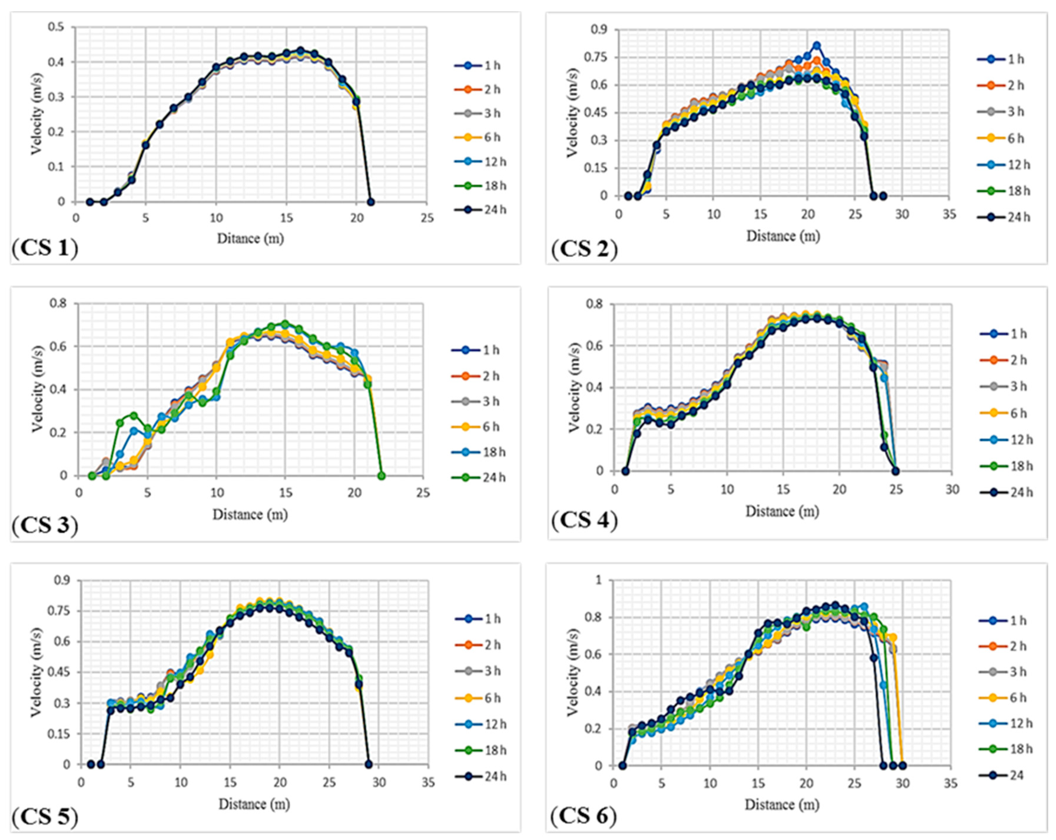
Figure 1. Location of Kurau and Ara river confluence.
Resources 08 00009 g001
Figure 2. Observed bathymetry survey of the Kurau-Ara rivers confluence.
Resources 08 00009 g002
Figure 3. Particle size distribution for the Kurau–Ara river confluence (a) at normal depths and (b) for the scouring zone.
Resources 08 00009 g003
Figure 4. Flowchart of the solver’s procedures.
Resources 08 00009 g004
Figure 5. Unstructured grid for the Kurau–Ara river confluence.
Resources 08 00009 g005
Figure 6. Simulation of velocity magnitude with the locations of the cross sections.
Resources 08 00009 g006
Figure 7. Simulated average flow velocity magnitude (m/s) within one day at cross sections CS 1, CS 2, CS 3, CS 4, CS 5, and CS 6.
Resources 08 00009 g007
Figure 8. Simulation of water surface elevation with measured locations at the Kurau–Ara confluence.
Resources 08 00009 g008
Figure 9. Depth simulation with the locations of measured cross-sections at the confluence of Kurau and Ara Rivers.
Resources 08 00009 g009
Figure 10. Simulated bed elevation (m) within one day at cross-sections CS 1, CS 2, CS 3, and CS 5.
Resources 08 00009 g010
Figure 11. Comparison of measured and simulated bed elevations at CS 1, CS 2, CS 3, and CS 5 with Q = 15 m3/s.
Resources 08 00009 g011
Figure 12. Comparison of measured and simulated bed elevations at CS 1, CS 2, CS 3, and CS 5 with Q = 43 m3/s.
Resources 08 00009 g012
Figure 13. Simulated flow depth without and with vanes at an angle of 15° for the study site (a) without obstacle; (b) in the first scenario; (c) in the second scenario; (d) in the third scenario.
Resources 08 00009 g013
Figure 14. Simulated flow depth without and with vanes at an angle of 30° for the study site (a) without obstacle; (b) in the first scenario; (c) in the second scenario; (d) in the third scenario.
Resources 08 00009 g014
Figure 15. Simulated velocity distribution with its vectors without and with vanes at an angle of 15° for the study site (a) without obstacle; (b) in the first scenario; (c) in the second scenario; (d) in the third scenario.
Resources 08 00009 g015
Figure 16. Simulated velocity distribution with its vectors without and with vanes at an angle of 30° for the study site (a) without obstacle; (b) in the first scenario; (c) in the second scenario; (d) in the third scenario.
Resources 08 00009 g016
Table 1. Comparison of simulated and measured average flow velocities.
No.Cross SectionsSimulated Mean Velocity (m/s)Mean Velocity Measured
1 h2 h3 h6 h12 h18 h24 hMean
1CS 10.3100.3120.3120.3150.3170.3200.3190.3150.319
2CS 20.5740.5620.5490.5380.5090.5080.5120.5360.582
3CS 30.4940.4970.4970.4980.4590.4860.4760.4870.586
4CS 40.5330.5310.5280.5180.5070.4950.4820.5130.572
5CS 50.5690.5690.5660.5570.5670.5580.5370.5600.580
6CS 60.6310.6050.6080.6100.6000.5930.5850.6050.699
Table 2. Statistical indices for measured and simulated average velocities.
Cross-SectionAverage Velocity (m/s)Error M-SAbsolute Value of ErrorsSquare of ErrorAbsolute Values of Errors Divided by MeasuredResults of Different Statistical Indices
Measured (M)Simulated (S)
CS 10.5820.5360.0460.0460.0020.079MAD0.054
CS 20.3190.3150.0040.0042 × 10−50.013MSE0.004
CS 30.5860.4870.0990.0990.010.169RMSE0.064
CS 40.5720.5130.0590.0590.0030.103MAPE8.877
CS 50.580.560.020.024 × 10−40.034
CS 60.6990.6050.0940.0940.0090.134
Sum. 0.3220.0250.533
Table 3. Errors between measured and simulated water levels.
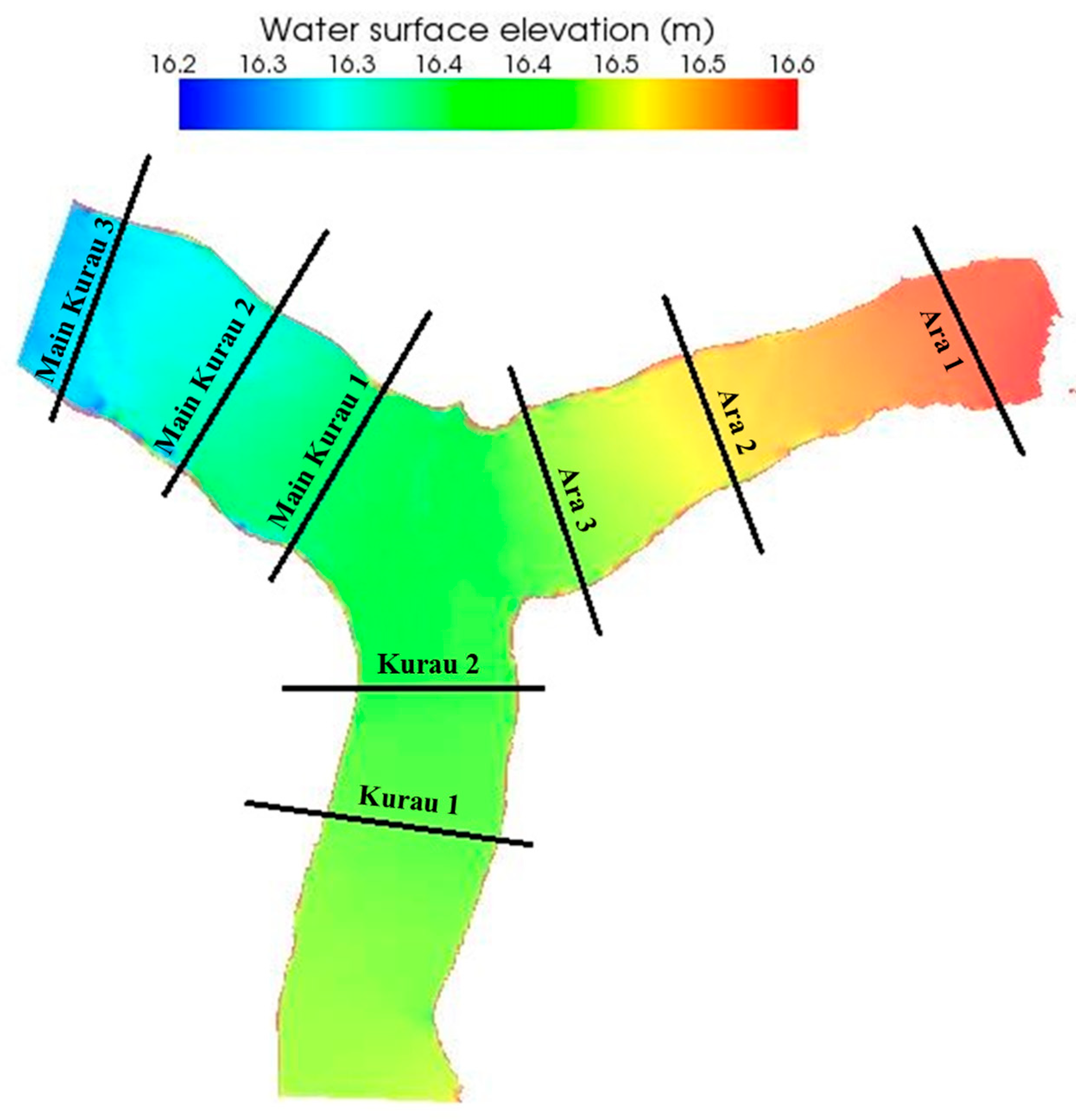
Location of Measuring Water Surface ElevationMeasured (m) a.m.s.lSimulated (m) a.m.s.lError M-SAbsolute Value of ErrorSquare of ErrorAbsolute Value of Error Divided by Measured
Kurau 116.47616.4410.0350.0350.00120.0021
Kurau 216.42316.432−0.0090.0098 × 10−50.0005
Ara 116.52816.578−0.050.050.00250.003
Ara 216.47516.514−0.0390.0390.00150.0024
Ara 316.42316.44−0.0170.0170.00030.001
Main Kurau 116.37116.386−0.0150.0150.00020.0009
Main Kurau 216.31816.33−0.0120.0120.00010.0007
Main Kurau 316.26616.278−0.0120.0120.00010.0007
Sum. 0.1890.00610.0115
Table 4. Discharges and water levels of Kurau-Ara River confluence used for model validation.
No.Time (s)Discharge (m3/s)Total Discharge (m3/s)Water Levels at Downstream of Main Kurau River (m)
Kurau RiverAra River
1054916.21
286,400871516.25
3172,80014173116.75
4259,20015284317.1
5345,60012233516.9
6432,00010152516.6
7518,400761316.2
Table 5. Comparisons of water levels and average flow depths for Q = 15 m3/s.
Transect NameWater LevelResults of Different Statistical IndicesAverage Flow Depth (m)Results of Different Statistical Indices
MeasuredSimulatedMeasuredSimulated
CS 116.4416.48MAD0.0321.171.12MAD0.04
CS 216.4516.49MSE0.0010.580.59MSE0.002
CS 316.4216.45RMSE0.0340.940.98RMSE0.044
CS 516.3816.4MAPE0.1980.780.84MAPE4.486
Table 6. Comparisons of water levels and average flow depths for Q = 43 m3/s.
Transect NameWater LevelResults of Different Statistical IndicesAverage Flow Depth (m)Results of Different Statistical Indices
MeasuredSimulatedMeasuredSimulated
CS 117.2917.35MAD0.0831.911.92MAD0.075
CS 217.317.37MSE0.0081.481.37MSE0.008
CS 317.21317.34RMSE0.0871.831.77RMSE0.087
CS 517.19317.27MAPE0.4841.581.7MAPE4.707
Table 7. Comparison of measured and simulated average flow velocities.
River NameDischarge (m3/s)Average Velocity (m/s)Confluence StatusMomentum Ratio (Mr) *
MeasuredSimulated
Ara70.490.5215 (m3/s)0.9
Kurau80.50.431
Ara280.850.75243 (m3/s)2.6
Kurau150.60.44
* Mr = (Q * U * ρ ) Ara/(Q * U * ρ ) Kurau.

