Tail-Risk Spillovers in Strategic Commodity and Carbon Markets: Evidence for Natural Resource Risk Management

Abstract

Commodity and carbon markets are central to natural resource allocation, energy security, and the effectiveness of carbon-pricing policies, yet their risk linkages can intensify sharply during crises. This study examines nonlinear, tail-dependent volatility spillovers across strategically important resource markets using a Quantile-on-Quantile connectedness framework. We employ weekly observed data from 3 January 2010 to 27 April 2025 for eleven futures markets spanning metals (copper, silver, gold), energy (WTI crude oil, heating oil, natural gas, gasoline), agricultural commodities (sugar, coffee, corn), and carbon emissions. Volatility is measured using GARCH-based estimates and embedded in quantile VAR dynamics to map state-contingent shock transmission across the distribution. The results indicate strong asymmetries: connectedness rises markedly in tail regimes and attains its highest levels during the COVID-19 pandemic and the Russia–Ukraine war, relative to the 2015–2016 energy market adjustment. Heating oil, gold, and natural gas frequently act as key volatility transmitters, while the carbon market shifts from a peripheral receiver to a more integrated and sometimes systemic node within the broader commodity risk network. The findings indicate that carbon-price risk propagates through resource markets in a regime-dependent manner, with implications for stress testing, tail-sensitive hedging, and the coordination of resource and climate policy under turbulent market states.

1. Introduction

Understanding how risk propagates across global commodity and carbon markets is essential for investors, policymakers, and regulators navigating an increasingly uncertain macro-financial environment. Strategic commodities, such as energy, metals, and agricultural products, form the backbone of global supply chains and are deeply intertwined with inflation dynamics [1], geopolitical developments [2,3], and structural transitions like decarbonization [4]. Meanwhile, carbon markets have increasingly assumed the characteristics of financialized commodities (traded futures contracts with speculative behavior, hedging value, and systemic importance), placing them alongside oil, gold, and natural gas in terms of risk interconnectivity [5,6,7].

The motivation for this study stems from three converging developments. First, recent crises, such as the COVID-19 pandemic, the Russia–Ukraine war, and energy market dislocations, have highlighted the asymmetric and nonlinear nature of risk transmission across commodity systems [8,9,10]. These episodes have reshaped the systemic roles of traditional hedging assets, such as gold, and emerging ones, like carbon emission futures [2,11]. Second, the integration of environmental assets into broader commodity-finance networks has increased. For example, carbon prices are increasingly co-moving with fossil fuel, metal, and agricultural markets, particularly under climate or geopolitical shocks [12,13,14]. This co-movement highlights carbon’s dual identity, as both an environmental asset and a financialized commodity, with implications for pricing, hedging, and contagion. Third, conventional mean-based connectedness frameworks fail to capture tail-risk and regime-dependent dynamics, particularly during extreme downside or exuberant market conditions, where quantile-specific spillovers dominate [4,15,16]. This study examines three linked questions. The first asks how volatility spillovers vary across normal, downside, and upside regimes. This is addressed by the quantile-on-quantile Total Connectedness surface, and the time-varying TCI reported for representative quantile states. The second asks which assets act as net transmitters and net receivers under lower-tail and upper-tail conditions. This is addressed by the net directional connectedness maps evaluated across quantile combinations and by the annual net connectedness summaries by quantile. The third asks how these transmission patterns change during major disruptions such as the 2015–2016 energy adjustment, the COVID-19 shock, and the Russia–Ukraine war. This is addressed by the crisis subperiod network summaries and the dynamic connectedness plots that track regime-dependent spillovers over time.

Carbon sequestration policies and subsurface decarbonization technologies increasingly interact with the circulation and exploitation of natural resources, creating an additional channel through which commodity and carbon risks may co-evolve. In practice, climate policy support for carbon capture and storage (CCS) can change the economics of extraction, reservoir management, and energy security, while also linking emissions pricing to operational decisions in upstream and midstream systems. Recent engineering evidence highlights that CO₂ can be used as an active working fluid in subsurface operations, including CO₂-based fracturing concepts applied to natural hydrogen reservoirs, where fracture propagation and reservoir imperfections affect stimulation efficiency and, consequently, project feasibility under decarbonization constraints [17]. At the same time, depleted gas reservoirs are increasingly discussed as strategic infrastructure that can move beyond CO₂ sequestration toward integrated applications such as hydrogen storage, reinforcing the role of subsurface assets in the energy transition and strengthening the policy-driven coupling between carbon management and resource markets [18]. These developments motivate treating carbon futures not only as a policy instrument but also as a market-based risk factor that can become more closely linked to commodity volatility during periods of climate-policy tightening or geopolitical stress.

Volatility spillovers across commodity and carbon markets can be interpreted through three complementary channels. The first is a value chain and inventory channel, in which shocks to production, refining, storage, and transportation propagate across linked contracts, especially in energy markets, where refined products embed both crude input costs and downstream demand conditions. The second is a financial channel, where margin requirements, funding constraints, and risk appetite interact with commodity futures positioning, amplifying co-movements when investors deleverage or rebalance across asset classes. The third is a policy and compliance channel specific to carbon markets, where expectations about emissions policy, compliance demand, and energy transition constraints interact with energy prices and industrial activity, thereby strengthening carbon’s linkage with commodity volatility under stress. These channels guide the interpretation of transmitter and receiver roles identified by the quantile-based connectedness analysis.

In constructing the agricultural segment of the system, we focus on corn, sugar, and coffee to capture the volatility dynamics of two economically important “soft” commodities (sugar, coffee) and a key grain (corn) that is frequently linked to inflation pressures and energy/biofuel channels, while maintaining a balanced 11-asset network across metals, energy, food, and carbon. This selection is also guided by the availability of long, liquid, and continuously traded futures series over the full 2010–2025 horizon, which is required for the rolling quantile-based connectedness estimation. We acknowledge that other agricultural contracts (e.g., wheat or soybeans) are also relevant for energy–agriculture linkages (e.g., ref. [19]) and represent a natural extension for future research.

To explore the research questions, we adopt a Quantile-on-Quantile (QQ) connectedness framework that integrates GARCH-based volatility estimates with quantile vector autoregressions (QVAR), enabling a state-contingent analysis of shock-response dynamics [20,21]. This approach enables us to identify asymmetric spillover patterns across different quantile regimes, particularly those associated with financial distress or speculative booms [5,22,23]. This study is framed as an exploratory investigation of tail-risk transmission rather than formal hypothesis testing. Nevertheless, interpretation is guided by empirical implications grounded in commodity-finance mechanisms. Gold is expected to become more influential during downside regimes when flight-to-safety and portfolio rebalancing intensify. Natural gas is expected to exhibit stronger spillover behavior in high-volatility and upside regimes given its sensitivity to demand surges, supply constraints, and geopolitical disruptions. Carbon futures are expected to become more integrated during periods of climate-policy tightening and energy-transition repricing, thereby strengthening their linkage to volatility in energy and industrial commodity markets. These implications are evaluated by comparing connectedness measures across lower-tail, median, and upper-tail quantiles and by examining event-specific subperiods.

This study contributes to the literature on systemic risk, volatility, connectedness, and climate-finance interlinkages in several empirical and design-based ways. First, it provides an integrated tail-risk connectedness assessment for a balanced commodity-carbon system spanning metals, the fossil-fuel value chain, agriculture, and carbon emissions futures, which supports cross-sector comparison within a single framework and complements recent multi-asset connectedness evidence in commodities and related markets [24,25]. Second, the paper does not claim a new estimator in a strict methodological sense; rather, it extends existing quantile connectedness implementations by explicitly modeling spillovers in a two-dimensional quantile setting, allowing the shock quantile and the response quantile to differ. By estimating a quantile-on-quantile connectedness surface, the analysis characterizes spillovers jointly as a function of the shock state and the response state, which differs from settings that summarize tail dependence using a small number of matched-quantile cases and aligns with evidence that spillovers intensify in tail regimes [11,20,26,27]. Third, the paper provides event-specific evidence by comparing connectedness patterns across major global disruptions, consistent with crisis-sensitive spillover dynamics documented for COVID-19 and the Russia–Ukraine war [8]. Fourth, the results clarify asset-level role switching across regimes, including gold’s dual safe-haven and transmission behavior and the asymmetric spillover profile of natural gas across quantiles, in line with related commodity-finance evidence [20,26,28]. Finally, the findings strengthen the interpretation of carbon futures as a market-based risk channel whose systemic position can evolve under climate policy and geopolitical stress, thereby complementing recent evidence on carbon’s increasing integration with commodity risk transmission [2,22].

Our empirical findings offer several policy-relevant insights. Volatility spillovers are highly asymmetric and quantile-dependent, aligning with the existing literature, which shows elevated spillovers during both distress and exuberance regimes [16,29]. The COVID-19 pandemic and the Russia–Ukraine war generated densely connected transmission networks across commodity sectors, whereas earlier events, such as the 2015–2016 energy correction, showed more sector-specific effects [8,30]. Carbon markets, in particular, became central risk hubs during recent crises, an evolution also observed by [2,13]. Moreover, directional connectedness varies over time, with natural gas and heating oil exhibiting alternating roles as transmitters and receivers under different quantile conditions [9,23]. For commodity traders and risk managers, these findings suggest that monitoring quantile-dependent transmitters, such as gold during downside shocks or natural gas during surges, can inform tail-risk hedging and dynamic portfolio allocation. Understanding which assets drive volatility under extreme regimes offers actionable intelligence for derivatives positioning and early-warning risk dashboards. These findings reaffirm the importance of state-contingent, event-sensitive connectedness frameworks for understanding systemic volatility across interconnected commodity and financialized environmental markets.

The remainder of this paper proceeds as follows: Section 2 reviews the related literature. Section 3 presents the methodological framework. Section 4 describes the data. Section 5 discusses the empirical results. Section 6 concludes.

2. Literature Review

The literature on volatility spillovers and systemic risk in commodity markets has expanded significantly in recent years, driven by heightened economic uncertainty and recurring global crises. This section synthesizes relevant studies under three main themes: (i) volatility spillovers across commodity sectors, (ii) quantile-based and tail-risk approaches, and (iii) crisis-driven connectedness dynamics. To improve positioning, we also relate our design more explicitly to the closest quantile and tail-event contributions and clarify what our framework adds in terms of cross-sector coverage, crisis comparability, and the mapping of spillovers across shock and response states.

2.1. Volatility Spillovers Across Commodity Sectors

Several studies have explored interdependencies across major commodity sectors using various connectedness and network-based methodologies. Ref. [28] conduct a broad analysis of contagion patterns among energy, agricultural, livestock, and metal futures during key global crises, identifying gold and silver as consistently dominant transmitters. Their findings align with those of [31,32], who emphasize the leading role of metal futures in shaping volatility transmission channels. In contrast, agricultural commodities often emerge as passive receivers, highlighting sectoral asymmetry in systemic behavior.

Ref. [33] advance this understanding by showing that crude oil, silver, and corn play fundamental roles as spillover sources, influencing both intra- and inter-sectoral linkages. Refs. [34,35] document strong bidirectional and asymmetric transmission between oil and agricultural markets, suggesting that supply-side shocks in one category can propagate across others. These findings emphasize the importance of accounting for dynamic feedback mechanisms. The systemic importance of specific commodities varies over time. Ref. [24] identify Soybean Oil, Cotton, and Coffee as primary transmitters in recent years, while Natural Gas and Heating Oil exhibit safe-haven behavior during high-stress episodes. Notably, ref. [36] find that energy commodities dominate systemic contributions in the post-COVID-19 period, except for natural gas, which exhibits distinct behavior. This strand documents sectoral heterogeneity and role switching, but much of the evidence remains difficult to compare across sectors when studies focus on a narrow subset of markets or report results under a single average regime.

Across commodity-sector studies, there is broad agreement that systemic roles are heterogeneous and can switch over time, with metals and parts of the energy complex frequently appearing as volatility hubs. However, the literature does not converge on a stable ranking of transmitters versus receivers because results are sensitive to the system’s sectoral coverage (energy-only versus multi-sector), the volatility proxy used, and whether dependence is assessed at the mean or under stress regimes. This limits cross-study comparability and leaves unresolved whether “dominant transmitters” reflect persistent structural importance or regime-specific behavior. These debates motivate our balanced cross-sector design and our regime-dependent connectedness mapping.

2.2. Quantile-Based and Tail-Risk Approaches

A growing strand of literature highlights the limitations of traditional mean-based connectedness models in capturing risk under extreme market conditions. Refs. [16,37] demonstrate that volatility spillovers intensify at both lower and upper quantiles, necessitating models that explicitly account for distributional asymmetries. Quantile VAR (QVAR) models and quantile-based network approaches have become instrumental in this context. Refs. [20,21] demonstrate that quantile-based frameworks indicate state-dependent transmission structures, particularly during periods of financial stress or exuberance. Ref. [15] apply these tools to clean energy, fossil energy, and metals, showing that mean-connectedness measures severely understate risks in tail regimes.

Further refinement is provided by [23,27], who introduce tail-event-driven network models (e.g., RTENET) that indicate how uncertainty reconfigures connectedness. Refs. [22,30] find that both the direction and intensity of spillovers vary across quantiles and frequencies, indicating the need for dynamic, multiscale approaches to volatility modeling. These closest studies motivate two design considerations that are central to our approach. First, quantile-based connectedness results depend on the market state, so cross-regime interpretation requires a coherent mapping across quantiles rather than isolated tail comparisons. Second, tail-event and quantile approaches often emphasize how connectedness changes under extremes, but they do not always distinguish between the state in which a shock originates and the state in which it is absorbed, even though these can differ in practice. Building on this insight, our quantile-on-quantile specification reports connectedness as a function of both the shock and response quantiles, yielding a connectedness surface rather than a small set of separate regime snapshots.

Quantile-based connectedness studies consistently indicate stronger spillovers under tail conditions, but the evidence remains mixed on whether downside and upside tails produce symmetric network structures and whether the same assets remain central across tails. A further unresolved issue is that many applications evaluate matched tail states only (e.g., lower-to-lower), which can obscure the practical case in which shocks originate under one state but transmit into a different state. This motivates our quantile-on-quantile specification, which separates the shock state from the response state, yielding a connectedness surface rather than isolated quantile snapshots.

2.3. Crisis-Driven Spillovers and Systemic Shocks

A substantial body of literature focuses on how global crises alter volatility spillover dynamics. Refs. [8,38] demonstrate that during events such as the COVID-19 pandemic and the Russia–Ukraine war, transmission patterns become more intense and intersectoral. Notably, assets such as oil and metals switch roles, from shock absorbers to key transmitters, highlighting the adaptive nature of systemic importance. Ref. [30] find that crude oil behaved as a net receiver during the war, contrary to its traditional role as a transmitter. Refs. [3,39] emphasize the role of conflict intensity, geopolitical exposure, and central bank actions in shaping these systemic transitions. Ref. [10] focus on higher-moment connectedness and document increased co-kurtosis and tail spillovers in response to geopolitical shocks.

In agricultural markets, crisis-induced patterns of connectedness are also evident. Refs. [19,26,40] report that commodities like wheat, corn, and soybeans become dominant transmitters during supply chain disruptions, indicating the vulnerability of food systems. Ref. [41] extend this perspective by linking international commodity volatility to systemic stress in China’s financial sector, further emphasizing global interdependence.

Despite the growing use of quantile and tail-risk connectedness tools in commodity and energy finance, existing evidence is still fragmented across markets and regimes. A substantial part of the literature examines spillovers within specific commodity segments or emphasizes a limited set of tail states, which can restrict cross-sector comparability and mask how spillovers change when the shock state and the response state differ across quantiles [16,20,23]. Moreover, recent crisis-focused studies show that systemic roles and spillover intensity can vary substantially across episodes such as COVID-19 and the Russia–Ukraine war, motivating an integrated framework to compare regimes and events within a single system [8,9,10].

Crisis-focused studies generally agree that connectedness rises sharply during systemic disruptions, yet they often differ in how crises are defined, how “before” benchmarks are chosen, and whether comparisons are made using consistent windows. This creates an unresolved debate about whether documented crisis effects reflect event-specific transmission or differences in window construction and sample composition. In response, we adopt fixed event windows and a consistent pre-event benchmark, allowing crisis-induced structural changes to be compared using the same connectedness objects.

2.4. Economic Mechanisms of Volatility Transmission

The empirical literature on connectedness is often interpreted through a set of economic mechanisms that explain why specific markets become volatility transmitters. Energy futures are linked by value-chain pass-through and inventory dynamics, meaning that shocks to refining margins, storage capacity, and transportation constraints can propagate across crude and refined products. In addition, commodity futures trading requires margining and collateral constraints, so funding and liquidity conditions can generate synchronized volatility when investors adjust exposures rapidly. Precious metals are frequently interpreted through hedging and safe-haven rebalancing channels, since periods of heightened uncertainty can trigger portfolio shifts that transmit volatility across commodities and related markets. Carbon markets introduce a distinct compliance-and-policy channel, where regulatory expectations and energy-transition constraints can interact with energy prices and industrial activity, thereby strengthening carbon’s connectedness during geopolitical and climate-policy shocks. This mechanism framework provides the economic basis for interpreting the quantile-dependent roles of the transmitter and receiver documented in the empirical section.

2.5. Contribution of the Study

Relative to closest-quantile and tail-event studies, the gap addressed here is not the absence of quantile methods, but the limited use of joint shock–response quantile mapping and of coherent cross-sector comparability in a single-commodity-carbon setting. More specifically, relative to closest-quantile and tail-event studies, our empirical design contributes by combining three elements within a single coherent framework. First, we implement a balanced cross-sector commodity-carbon system that enables direct comparison of role switching across metals, the fossil-fuel value chain, agriculture, and carbon emissions within the same estimation environment. Second, we estimate a quantile-on-quantile connectedness surface that maps spillovers across combinations of shock and response quantiles, addressing the practical case in which shocks arise in one state but transmit to another. Unlike recent quantile-connectedness applications that focus mainly on matched-quantile cases (e.g., lower–lower, median–median, upper–upper) or a small set of tail snapshots, our design explicitly separates the quantile state in which shocks originate from the quantile state in which they are absorbed. This point clarifies the paper’s differentiation from studies that focus primarily on matched-quantile transmission or a small set of tail states. This separation is empirically relevant because crisis transmission can be asymmetric across these two dimensions, so spillovers may originate under downside states but propagate into median or upper-tail responses, which cannot be identified from matched-quantile reporting alone. Third, we align crisis comparisons using fixed event windows and a consistent “before” benchmark, allowing the same connectedness objects to be contrasted across episodes in a transparent way. In response, this study constructs a balanced cross-sector system spanning metals, the fossil-fuel value chain, agriculture, and carbon emissions futures, and estimates a quantile-on-quantile connectedness surface that maps volatility spillovers across combinations of shock and response quantiles. This design provides regime-specific risk maps, identifies transmitter–receiver role switching across tails, and documents event-dependent changes in carbon’s systemic position. Accordingly, the paper’s contribution should be interpreted as an application and an extension of evidence: it produces regime-specific risk maps, documents transmitter–receiver role switching across tails, and tracks event-dependent changes in carbon’s systemic position, without claiming a theoretical breakthrough in the connectedness methodology itself.

3. Research Methodology

3.1. Volatility Estimation

To estimate time-varying volatility for each asset, we first specify the return process as:

$${ret}_t={\mu }_t+\delta {ret}_{t-1}+{\epsilon }_t$$

(1)

where ${\mu }_t$ denotes a constant drift, $\delta$ captures autoregressive dynamics, and ${\epsilon }_t$ represents the innovation term. The conditional volatility for the asset $i$ is then modeled via a GARCH (1,1) process:

$${\sigma }_{i,t}^2=c+\alpha {\epsilon }_{i,t-1}^2+\beta {\sigma }_{i,t-1}^2$$

(2)

The parameters satisfy $c>0,\alpha \ge 0,\beta \ge 0,$ and $\alpha +\beta <1$, ensuring positive and stationary conditional variances. This formulation captures persistence in volatility and facilitates robust estimation of systemic risk metrics in subsequent quantile-based analyses.

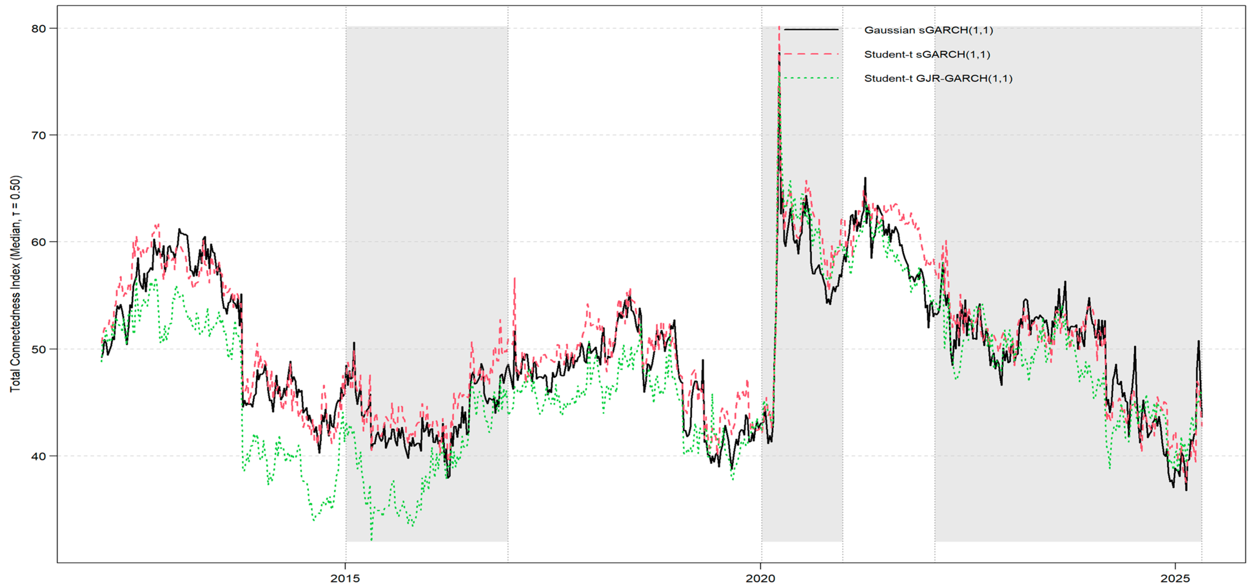
We estimate conditional volatilities using a standard GARCH (1,1) specification with Gaussian innovations. This choice is motivated by its parsimony, stable convergence in large multivariate settings, and its established performance as a benchmark volatility filter in commodity-market applications, particularly when the objective is to construct a consistent volatility proxy for subsequent multivariate spillover analysis rather than to model leverage effects at the univariate level. While asymmetric (EGARCH/GJR-GARCH) and long-memory (FIGARCH) specifications may capture additional features such as sign-dependent responses and persistent volatility, our quantile-based connectedness framework is designed to capture tail-dependent and state-contingent transmission mechanisms directly through the QVAR structure. Moreover, introducing heterogeneous volatility filters across assets can confound cross-series comparability in the connectedness stage.

3.2. Quantile ADF and Quantile PP Tests

To examine the stationarity properties of the volatility series across different distributional regimes, we apply the Quantile Augmented Dickey–Fuller (QADF) and Quantile Phillips–Perron (QPP) tests. Unlike traditional unit root tests that assess mean-level behavior, these quantile-based approaches allow us to investigate whether the persistence of shocks varies across different parts of the distribution, particularly under tail risk conditions such as market distress or exuberance. The QADF test transforms each series into a quantile process using the indicator-based formulation proposed by [42], where the test statistic is derived from:

$${\phi }_t^{\left(\tau \right)}=\tau -I\left(y_t\le q_{\tau }\right)$$

(3)

With $I\left(.\right)$ being the indicator function and $q_{\tau }$ the empirical quantile at level $\tau$. We compute ADF test statistics across a grid of quantiles $\tau \in \left\{0.05,0.10,\dots ,0.95\right\}$ with automatic lag selection. To ensure robustness, we also conduct Quantile Phillips–Perron tests on the same transformed series, applying the nonparametric Z-tau statistic under the assumption of a constant mean and short lag truncation. The use of both QADF and QPP tests enables us to confirm whether the unit root behavior observed is sensitive to distributional tails or is consistent across quantiles.

3.3. Quantile-on-Quantile Risk Transmission

To capture the asymmetric and state-dependent nature of risk spillovers across strategic commodity and carbon markets, this study adopts the Quantile-on-Quantile (QQ) risk transmission framework, as developed by [43]. The methodology extends the standard Quantile Vector Autoregressive (QVAR) model by incorporating quantile-specific interdependencies between shocks and responses across the distribution. This enables the identification of nonlinear and regime-contingent volatility transmission mechanisms. Formally, the QQ risk transmission model is built upon a QVAR(p) specification as follows:

$$x_t=\mu \left(\tau \right)+{\sum }_{j=1}^p{B}_j\left(\tau \right)x_{t-j}+u_t\left(\tau \right)$$

(4)

where $x_t$ is a $K\times 1$ vector of endogenous variables (volatility series), $\mu \left(\tau \right)$ is the quantile-specific intercept, $B_j\left(\tau \right)$ are the quantile-dependent coefficient matrices, and $u_t\left(\tau \right)$ is the vector of error terms. The parameter $\tau \in \left[0,1\right]$ denotes the quantile level, allowing the system to capture heterogeneous dynamics across different market states (e.g., distress, calm, exuberance). Using Wold’s decomposition, the QVAR(p) model is transformed into its quantile-specific vector moving average (QVMA) representation:

$$x_t=\mu \left(\tau \right)+{\sum }_{i=0}^{\infty }{A}_i\left(\tau \right)u_{t-i}\left(\tau \right)$$

(5)

The generalized forecast error variance decomposition (GFEVD) is then applied to the QVMA representation to estimate the proportion of forecast error variance in variable $i$ attributable to shocks in variable $j$ over a forecast horizon $F$:

$${\varnothing }_{i\leftarrow j,\tau }^g\left(F\right)={\displaystyle \frac{{\sum }_{f=0}^{F-1}{\left(e_i^{\prime }{A}_f\left(\tau \right)H\left(\tau \right)e_j\right)}^2}{H_{ii}\left(\tau \right){\sum }_{f=0}^{F-1}\left(e_i^{\prime }{A}_f\left(\tau \right)H\left(\tau \right)A_f{\left(\tau \right)}^{\prime }{e}_i\right)}}$$

(6)

To ensure interpretability, the decomposition is normalized, yielding the scaled GFEVD:

$${gSOT}_{i\leftarrow j,\tau }\left(F\right)={\displaystyle \frac{{\varnothing }_{i\leftarrow j,\tau }^g\left(F\right)}{{\sum }_{j=1}^k{\varnothing }_{i\leftarrow j,\tau }^g\left(F\right)}}$$

(7)

This scaled measure is then used to compute the directional spillovers to and from each asset. The total directional connectedness from variable i to all others is:

$$S_{i\to ·,\tau }^{gen,to}={\sum }_{k=1,i\ne j}^k{gSOT}_{k\leftarrow i,\tau }$$

(8)

And the directional connectedness received by variable i from all others is:

$$S_{i\leftarrow ·,\tau }^{gen,from}={\sum }_{k=1,i\ne j}^k{gSOT}_{i\leftarrow k,\tau }$$

(9)

The net directional connectedness of asset i capturing its role as a transmitter or receiver of risk, is computed as:

$$S_{i,\tau }^{gen,net}=S_{i\to ·,\tau }^{gen,to}-S_{i\leftarrow ·,\tau }^{gen,from}$$

(10)

A positive $S_{i,\tau }^{gen,net}$ implies that asset i is a net transmitter of systemic volatility at quantile $\tau$, while a negative value indicates it is a net receiver. Aggregating across all nodes yields the Total Connectedness Index (TCI), a measure of systemic interdependence within the network at a specific quantile:

$${TCI}_{\tau }\left(F\right)={\displaystyle \frac{k}{k-1}}{\sum }_{k=1}^k{S}_{i\leftarrow ·,\tau }^{gen,from}\equiv {\displaystyle \frac{k}{k-1}}{\sum }_{k=1}^k{S}_{i\to ·,\tau }^{gen,to}$$

(11)

This quantile-on-quantile GFEVD-based approach allows us to construct directional, net, and total connectedness measures across all quantile combinations of shocks and responses. In doing so, it provides a richer and more granular understanding of systemic risk transmission, particularly during periods of financial turbulence, inflationary surges, and energy or climate-related shocks.

Commodity and carbon markets span multiple crisis and transition regimes over the 2010–2025 window, so parameter stability cannot be assumed. We address this concern directly through a rolling-window quantile VAR connectedness design, which allows the spillover structure to change over time rather than imposing a single fixed set of relationships for the full sample. In addition, we report episode-based comparisons aligned with major disruptions such as the 2015–2016 energy market adjustment, the COVID-19 episode, and the Russia–Ukraine war period to show how connectedness changes across regimes.

The connectedness measures are model-implied dependence indicators and are interpreted as descriptive summaries of state-dependent spillover intensity. While the framework identifies regime differences and role switching, the paper does not claim formal hypothesis testing for individual edges. The empirical conclusions are therefore supported through multiple robustness exercises rather than statistical significance tests.

4. Data Description

This study uses weekly futures price data from 3 January 2010, to 27 April 2025, covering eleven strategically selected contracts across commodities and carbon markets. All series are collected from Investing.com and converted to a weekly frequency. The selection includes assets that are central to global production, consumption, and environmental regulation, allowing for a comprehensive examination of systemic risk transmission across heterogeneous sectors. Similar to the diversified datasets used in [2,24,28], this cross-sectoral composition enables us to capture the evolving nature of volatility connectedness across interlinked asset classes. The dataset comprises metals (copper, silver, gold), energy commodities (WTI crude oil, heating oil, natural gas, gasoline), agricultural commodities (sugar, coffee, corn), and carbon emission futures. Metals are selected due to their dual role as industrial inputs and financial hedging instruments. Gold and silver are widely documented as safe havens during crises [28,35], while copper is often seen as a proxy for global economic activity [32,33].

Energy commodities represent key segments of the fossil fuel value chain, capturing upstream (crude oil), midstream (natural gas), and downstream (heating oil and gasoline) activities. These assets are susceptible to geopolitical risk and macroeconomic shocks, as evidenced in [8,10,30]. Crude oil, in particular, has exhibited variable systemic roles depending on the nature and intensity of crises [3,9]. Agricultural commodities, such as sugar, coffee, and corn, are included because they are susceptible to inflationary shocks and climate change and are increasingly linked to energy markets through biofuel demand [7,26,40]. These assets have also shown spillover potential during periods of supply chain disruption and food insecurity [19,41].

Carbon emission futures are included to reflect the increasing financialization of environmental markets and the systemic integration of climate risk into global capital flows. Prior research highlights the dynamic interactions between carbon markets and both traditional commodities and policy uncertainty indices [2,5,44]. Their inclusion aligns with recent studies emphasizing the strategic role of carbon as both a transmitter and a receiver of systemic shocks, particularly during periods of climate or geopolitical stress [13,14] (Carbon emission futures are proxied by the Carbon Emissions futures series from Investing.com (identifier: CFI2H6), which is reported as an ICE-traded contract. This choice provides a transparent, continuously observed benchmark for carbon-price risk within the commodity system and facilitates full replicability of the dataset’s construction. The contract metadata reported on the same page indicates physical settlement and a contract size of 1000 tonnes, and it also reports the rollover schedule through the last rollover day shown for the active contract. We acknowledge that liquidity and rolling conventions can influence futures-based measures; therefore, we emphasize that the objective is to study system-wide volatility transmission using a consistent, transparent data construction across markets rather than to infer microstructure-level effects).

The period from January 2010 to April 2025 is selected to encompass multiple commodity cycles and policy regimes central to this paper’s motivation. These include the post-global financial crisis normalization phase, the 2015–2016 energy market adjustment, the COVID-19 shock, and the Russia–Ukraine war. Weekly sampling is used to align information across heterogeneous futures contracts and to obtain volatility measures that are less affected by short-lived microstructure effects and asynchronous trading than daily series, consistent with the methodologies of [16,23]. Weekly frequency is also preferred because it improves comparability across markets with different trading hours, holiday calendars, and liquidity conditions, and it limits the influence of thin-trading effects that can distort higher-frequency volatility inputs in multi-asset systems. At the same time, we acknowledge that weekly aggregation can smooth very short-term spillovers during fast-moving episodes. The objective of this study is therefore to characterize regime-dependent and crisis-sensitive spillovers at a macro-financial horizon rather than intraday contagion. Extending the analysis to daily (or intraday) frequency, when consistently available for all contracts, is a natural direction for future research. This frequency also supports stable rolling-window QVAR estimation by reducing excess noise while preserving medium-run dynamics relevant to systemic spillovers. The eleven contracts are chosen to form a balanced cross-sector network that captures industrial and safe-haven metals (copper, silver, gold), the fossil-fuel value chain (WTI, heating oil, natural gas, gasoline), and inflation- and climate-sensitive agricultural markets with energy and biofuel linkages (corn, sugar, coffee). Carbon emissions futures are included as the market-based instrument most directly linked to carbon pricing and climate policy regimes.

Table 1. Descriptive Statistics of the Variables.

	Copper	Silver	Gold	OIL WTI	Heating Oil	Natural Gas	Gasoline	Sugar	Coffee	Corn	Carbon
Mean	0.00040187	0.000704993	0.001334067	−0.000442975	−0.000013	−0.000474476	−0.000098	−0.000498145	0.001265175	0.000079	0.00210935
Median	0.000738514	0.001024415	0.002082714	0.002086128	0.000899865	−0.001842833	0.00170146	−0.001246494	−0.000617665	0.00148809	0.00385356
Min	−0.18125261	−0.32008833	−0.101345882	−0.346863257	−0.290679758	−0.285999164	−0.434833864	−0.134247605	−0.160293744	−0.25305979	−0.41293978
Max	0.142469762	0.160145895	0.105756916	0.275756291	0.241884788	0.296326927	0.270292918	0.112596129	0.18630456	0.13722056	0.23243091
Std_Dev	0.031823021	0.042571095	0.02179112	0.051473185	0.044622923	0.075067833	0.05482716	0.034409789	0.042841984	0.03794879	0.06481748
Skewness	−0.19934026	−1.102891329	−0.198650525	−0.473534226	−0.43630957	−0.226100125	−0.683374489	−0.03593608	0.206801988	−0.53341512	−0.77428172
Kurtosis	5.480449405	11.20034066	5.031958208	8.792926323	7.209870484	4.568186209	12.61769516	3.527241765	3.810473539	6.60375112	7.45460872
Jarque_Bera	208.0190 ***	2376.660 ***	141.2825 ***	1135.577 ***	609.2174 ***	87.7908 ***	3110.214 ***	9.332135 ***	27.28737 ***	465.541 ***	733.045 ***

Note: This table reports descriptive statistics for weekly return series of the eleven futures contracts in the sample (3 January 2010, to 27 April 2025). Mean, Median, Min, Max, Standard Deviation, Skewness, and Kurtosis are computed from the weekly returns. The Jarque–Bera statistic tests the null hypothesis of normality; *** denotes statistical significance at the 1% level.

presents the descriptive statistics of the weekly return series for the selected commodities and carbon futures.

Average returns are generally close to zero across all assets, consistent with the typical behavior of stationary financial time series. However, the dispersion varies notably, with natural gas, gasoline, and crude oil (WTI) exhibiting the highest standard deviations, indicating elevated volatility in the energy sector. Carbon futures also exhibit considerable variability, indicating increasing sensitivity to climate-related market forces. Skewness values indicate asymmetry in the distribution of returns, with most series exhibiting negative skewness, particularly for corn, carbon, and silver, which suggests a higher probability of extreme negative returns. Meanwhile, kurtosis values exceed the benchmark of three in all series, confirming leptokurtic distributions and the presence of fat tails. These findings are further supported by Jarque–Bera statistics, which are statistically significant at the 1% level for all series, thereby rejecting the null hypothesis of normality. The descriptive statistics indicate non-normal, heavy-tailed return distributions, thereby justifying the use of quantile-based methods to uncover tail-dependent and nonlinear spillover dynamics in subsequent analysis.

5. Empirical Results and Discussion

5.1. Pre-Test Diagnostics

Before implementing the quantile-based connectedness analysis, we conduct a set of pre-test diagnostics to assess the underlying properties of the volatility series. Specifically, we employ the Pearson correlation matrix to examine aggregate linear associations, the BDS test to detect nonlinear dependence structures, and the Quantile ADF and PP tests to evaluate stationarity across the conditional distribution. These diagnostics provide crucial justification for adopting a nonlinear, quantile-aware framework.

5.1.1. Correlation Matrix

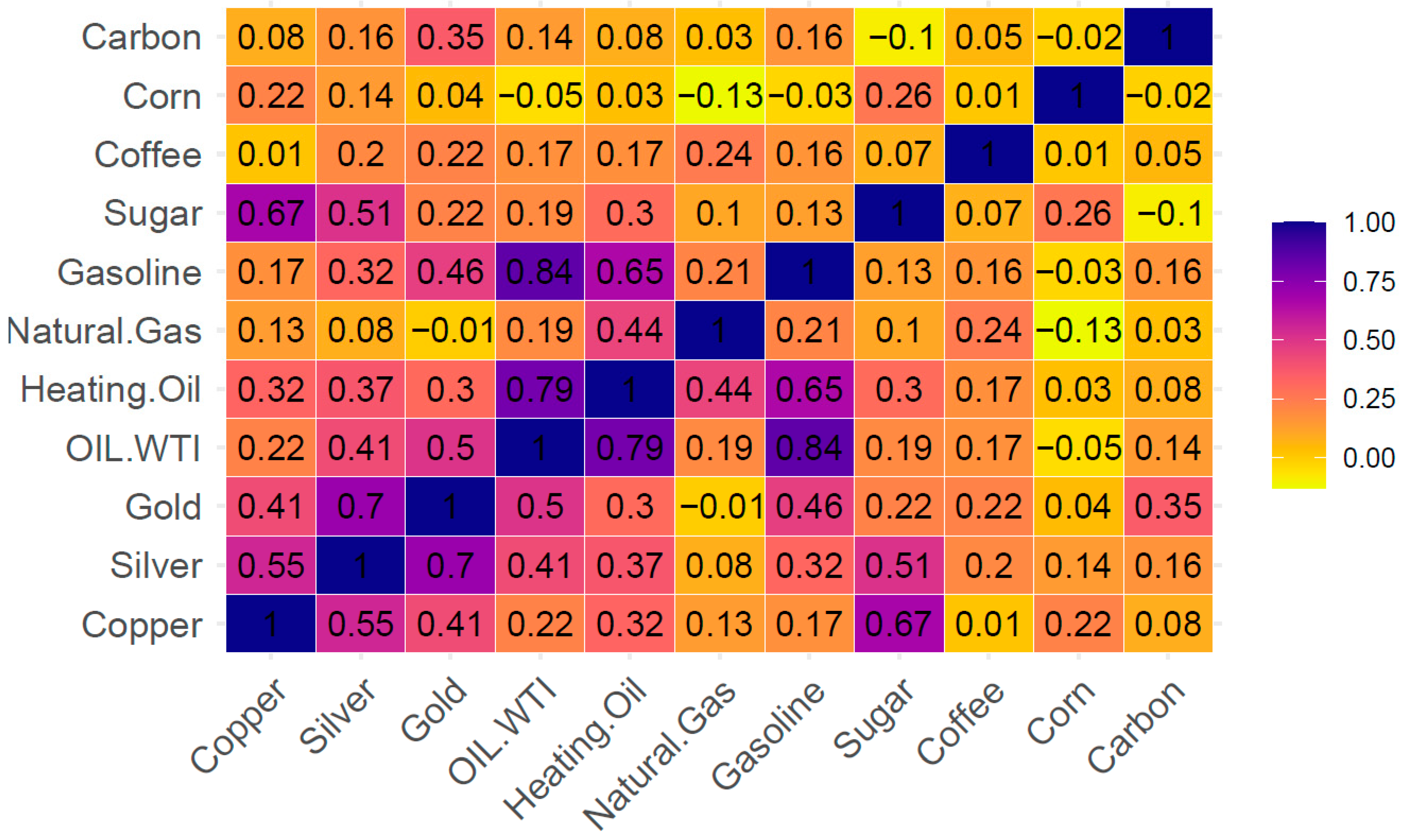
Figure 1 displays the Pearson correlation matrix of weekly GARCH (1,1) volatility estimates across the eleven selected commodities.

The results suggest mostly weak to moderate linear associations among the assets. The majority of correlation coefficients fall below 0.50, with many near zero and some even negative (e.g., Carbon with Sugar = −0.10, Corn with Heating Oil = −0.13), reflecting a diverse set of market dynamics. These weak correlations highlight the absence of strong co-movement in volatility at the aggregate level across most pairs. However, several clusters of stronger positive associations do emerge. Notably, Copper and Silver (ρ = 0.55), Gold and Silver (ρ = 0.70), and Heating Oil with Crude Oil (ρ = 0.79) show elevated correlation, likely reflecting structural or sectoral interdependencies, such as within precious metals or refined energy markets. Gasoline also displays strong links with Heating Oil (ρ = 0.65) and Crude Oil (ρ = 0.84), reinforcing its sensitivity to upstream energy shocks.

Despite these pockets of stronger co-movement, the overall structure of the matrix indicates considerable heterogeneity in how volatility propagates across commodity types, energy, metals, agriculture, and carbon. These findings reinforce the motivation to employ quantile-based, non-linear econometric frameworks. Simple correlation fails to capture the complexity of volatility interdependence, especially during extreme market conditions. Therefore, the application of Quantile-on-Quantile approaches is appropriate for uncovering asymmetric spillover patterns and tail-dependent dynamics that remain obscured in mean-based correlation metrics.

5.1.2. BDS Non-Linearity Test

Table 2. BDS Test Results for Nonlinearity Detection.

	Copper	Silver	Gold	OIL WTI	Heating Oil	Natural Gas	Gasoline	Sugar	Coffee	Corn	Carbon
M2	139.1571 ***	84.5947 ***	76.6574 ***	67.0634 ***	93.2266 ***	118.1964 ***	52.1505 ***	120.4435 ***	119.3208 ***	61.8398 ***	94.299 ***
M3	139.2937 ***	84.5091 ***	76.5446 ***	67.0508 ***	93.5063 ***	117.4663 ***	52.0148 ***	120.8327 ***	120.115 ***	61.5065 ***	94.305 ***
M4	139.4986 ***	84.4276 ***	76.5094 ***	67.1323 ***	93.3319 ***	116.7637 ***	51.8564 ***	121.3399 ***	120.7208 ***	61.1445 ***	94.429 ***
M5	139.8464 ***	84.362 ***	76.6919 ***	67.0204 ***	93.1429 ***	116.0668 ***	51.5283 ***	121.7608 ***	121.0894 ***	61.0692 ***	94.673 ***
M6	141.0062 ***	85.0615 ***	76.5779 ***	67.1273 ***	92.8127 ***	115.4603 ***	51.8323 ***	122.1616 ***	121.49 ***	60.7388 ***	94.705 ***

Note: This table reports the BDS (Brock–Dechert–Scheinkman) test statistics for detecting nonlinearity in the GARCH (1,1)-based volatility series of 11 commodity and carbon assets. The test is applied at embedding dimensions M2 to M6. The null hypothesis assumes the data are independently and identically distributed (i.i.d.). Rejection of the null hypothesis indicates the presence of nonlinear dependence. Statistical significance is denoted as follows: *** p < 0.01.

presents the results of the BDS (Brock–Dechert–Scheinkman) test applied to the volatility series of all eleven commodities across embedding dimensions from M2 to M6.

The results strongly reject the null hypothesis of independent and identically distributed residuals at the 1% level for all variables and dimensions, as indicated by the highly significant test statistics. This widespread rejection provides robust evidence of nonlinearity in the volatility dynamics of each commodity. Notably, Copper, Silver, and Natural Gas consistently exhibit among the highest BDS statistics across all embedding dimensions, indicating robust nonlinear signatures. These findings suggest that standard linear models would be inadequate for capturing the interdependencies in the data. The presence of significant nonlinear dynamics in all series further justifies the use of nonlinear, quantile-aware econometric tools. These models are better suited to capturing asymmetric spillovers and tail-dependent interactions that linear methods may overlook, particularly during episodes of market stress or exuberance.

5.1.3. Quantile ADF and PP Tests

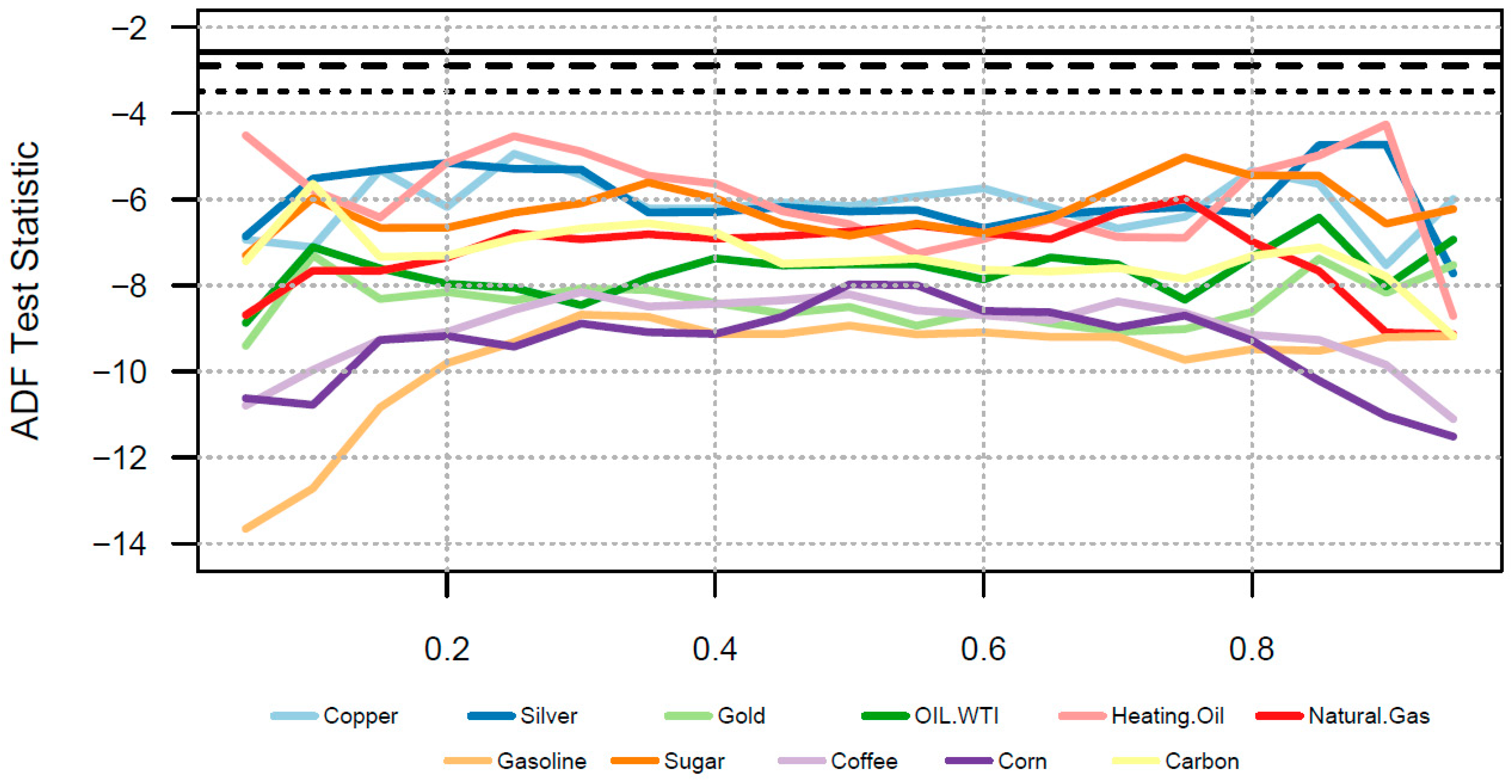
To assess the stationarity of the volatility series across different parts of the distribution, we apply the Quantile Augmented Dickey–Fuller (QADF) and Quantile Phillips–Perron (QPP) tests following [42]. These tests provide a distribution-sensitive evaluation of unit roots, helping to detect state-dependent persistence that may not be visible through traditional approaches. Figure 2 illustrates the QADF test statistics across quantiles for each of the 11 commodity and carbon volatility series.

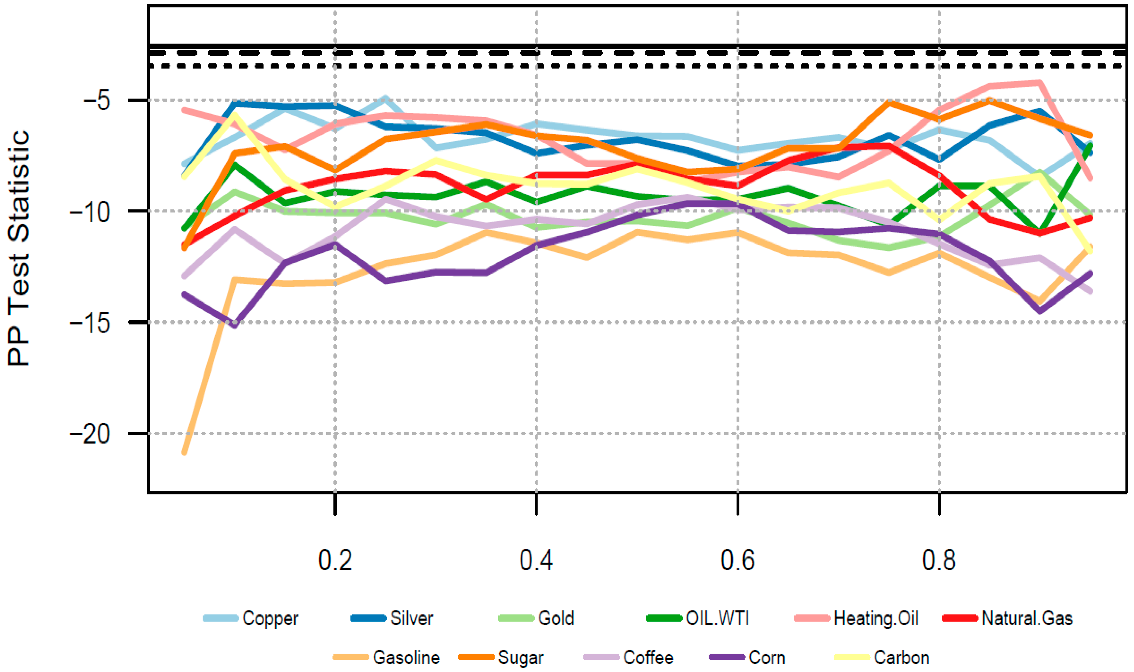
Figure 2 indicates that all test statistics consistently fall below the conventional 1%, 5%, and 10% critical values (depicted as horizontal lines), indicating that the null hypothesis of a unit root is rejected at all quantiles. Notably, the strength of stationarity varies by quantile and asset. For instance, Corn and Coffee exhibit especially strong stationarity in lower quantiles, with QADF statistics dropping below −10, while Silver and Heating Oil show relatively milder stationarity near the median quantiles. These results confirm that despite potential asymmetries in volatility behavior, the volatility series remain stationary across the distribution. Figure 3 presents the corresponding Quantile Phillips–Perron (QPP) test results.

Similar to the QADF outcomes, the QPP statistics fall consistently below the critical value thresholds across all quantiles. Gasoline and Corn again show pronounced rejection of the unit root, particularly in the lower and upper tails, suggesting strong mean reversion in periods of extreme volatility. In contrast, Gold and WTI exhibit slightly flatter profiles, suggesting more stable stationarity across quantiles, although they do not exhibit extreme values. Both the QADF and QPP tests provide strong evidence of quantile-dependent stationarity in the GARCH-based volatility series. These findings justify adopting quantile-based econometric approaches in the subsequent connectedness analysis, as they capture the nonlinear and state-contingent properties embedded in the data.

Across the full quantile grid, the QADF and QPP statistics reject the unit-root null for all eleven volatility series at conventional significance levels. This indicates that the GARCH (1,1)-based volatility measures are stationary across the conditional distribution, thereby supporting the stationarity assumption underlying the subsequent QVAR-based connectedness analysis. The quantile stationarity results imply that the volatility process is mean-reverting across the entire conditional distribution, including the lower and upper tails. This means that even during extreme market episodes, volatility does not exhibit explosive persistence that would distort cross-market transmission measurement. From an economic perspective, volatility shocks can be large and clustered, yet remain bounded and eventually revert, consistent with crisis-driven but transitory risk amplification. This is relevant for the quantile VAR stage because connectedness measures rely on a stable dependence structure in the modeled volatility series. Accordingly, the QADF and QPP outcomes provide direct support for the validity of the subsequent QVAR-based spillover estimation.

5.2. Risk Transmission Connectedness Network

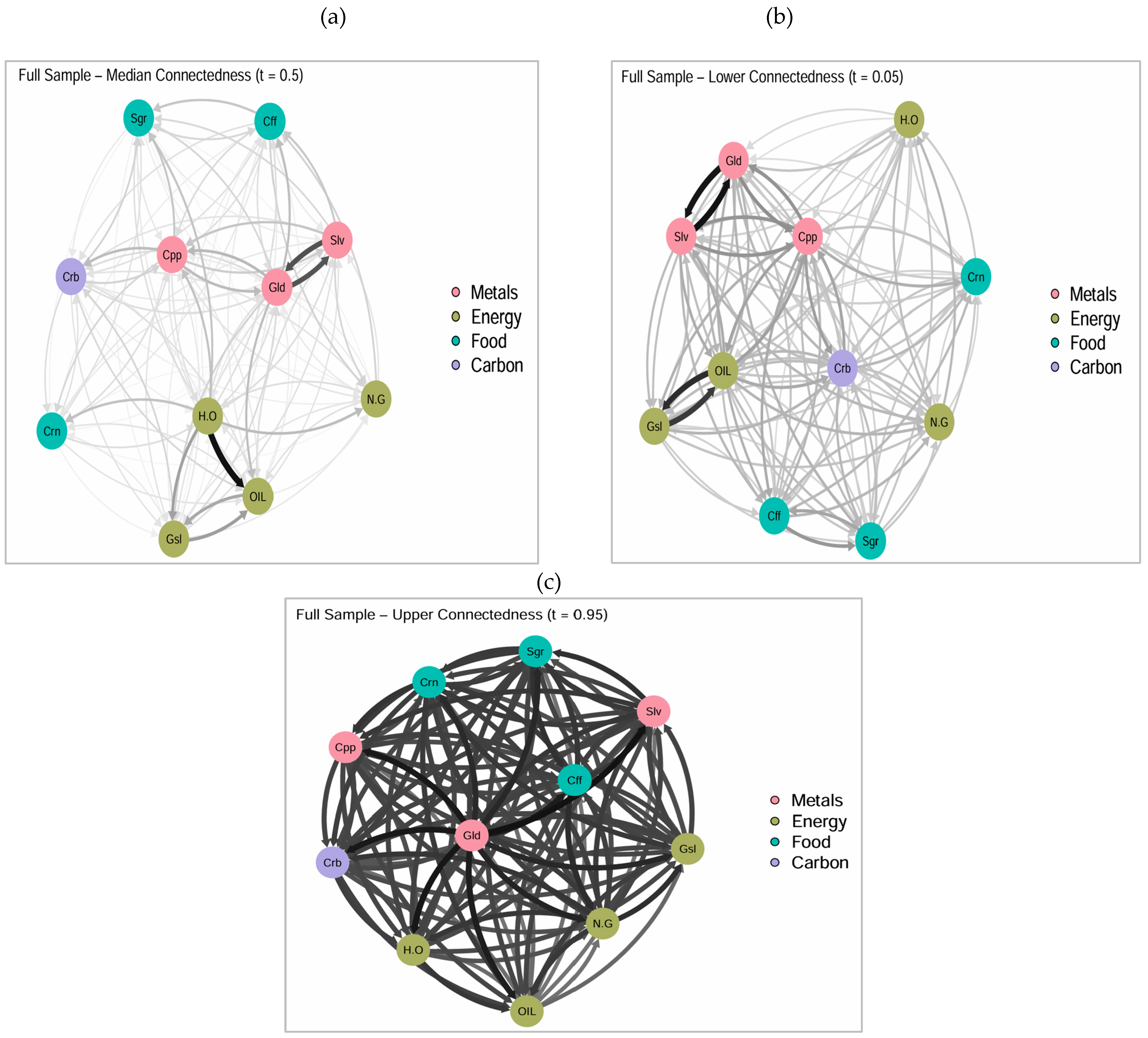
The quantile networks summarize how volatility shocks propagate across the resource system under different states. The transmitter role of precious metals in the lower tail is consistent with flight-to-safety rebalancing and the use of gold and silver as hedging assets, which can generate strong volatility spillovers when investors simultaneously adjust positions across commodity exposures. In energy markets, refined products and natural gas can transmit volatility through inventory and margin channels because disruptions to refining capacity, storage, and transportation affect multiple points along the fossil-fuel value chain. Carbon futures can become more closely linked during crisis episodes, when policy uncertainty, compliance expectations, and energy-price shocks jointly affect emissions costs and hedging demand, thereby strengthening the linkage between carbon pricing and conventional commodity volatility. To compare dependence structures across episodes, we use pre-specified crisis windows that correspond to widely documented market disruptions. The COVID-19 window encompasses calendar year 2020, capturing the global demand shock and commodity price dislocations. The Russia–Ukraine war window began in early 2022, reflecting the shift toward persistent geopolitical supply risk. For each event, the “before” window is defined as the preceding year to ensure comparable length and to limit confounding from long-run regime drift. In addition to the baseline GARCH volatility filter, we replicate the crisis-period connectedness patterns using weekly realized volatility, confirming that the main transmitter–receiver rankings are not driven by the volatility proxy. Figure 4 visualizes the quantile-dependent connectedness networks across 11 commodity and carbon assets, disaggregated by three quantile levels: median (τ = 0.5), lower tail (τ = 0.05), and upper tail (τ = 0.95). The networks are based on the average directional connectedness across the full sample period and grouped into four sectors: metals, energy, food, and carbon.

Figure 4 presents the quantile-based full-sample connectedness networks among commodity and carbon markets, capturing how systemic relationships evolve under normal, adverse, and exuberant market conditions. At the median quantile (τ = 0.5), the network is relatively sparse, with moderate transmission paths largely restricted within individual sectors. A notable feature is the strong bilateral linkage between gold and silver, reflecting their co-movement as dual-function assets that serve as both investment hedges and industrial inputs. This finding is consistent with those of [11,28], who highlight the persistent gold-silver pairwise transmission during periods of both typical and extreme volatility. Within the energy sector, heating oil emerges as a primary transmitter of volatility to crude oil and gasoline, indicating its central role in conveying demand-side signals. This pattern is consistent with energy value-chain pass-through, where refined product volatility reflects both upstream crude conditions and downstream demand and inventory adjustments, so shocks in heating oil can transmit to crude oil and gasoline through refining and storage linkages. Ref. [23] similarly emphasize the centrality of heating oil under bullish market regimes. Meanwhile, food commodities and carbon markets exhibit weak systemic integration under average conditions, implying limited spillover activity.

Under lower-tail shocks (τ = 0.05), which correspond to distress episodes or downside volatility, the network becomes markedly denser and more directional, signaling intensified contagion. Gold and silver continue to serve as dominant transmitters of volatility, reaffirming gold’s conventional role as a safe-haven asset during periods of financial turmoil. A plausible mechanism is flight-to-safety and hedging-driven reallocation under stress, where shifts into precious metals coincide with broad deleveraging and margin-related adjustments across futures positions, increasing the probability that volatility shocks transmit beyond the metals sector. This aligns with the findings of [16,45], who report stronger spillovers from precious metals during periods of geopolitical unrest and downside risk. Gasoline also emerges as a significant source of volatility, channeling adverse demand conditions to both crude oil and heating oil. Furthermore, carbon markets gain systemic relevance in this regime, potentially reflecting their exposure to ESG-driven capital flows and policy-related uncertainties. This finding aligns with [7,46], who demonstrate that climate policy uncertainty and ESG factors intensify the role of carbon markets during distress episodes. The denser lower-tail structure is consistent with broad deleveraging and margin-related position adjustments that tend to tighten cross-market volatility linkages when downside risk dominates.

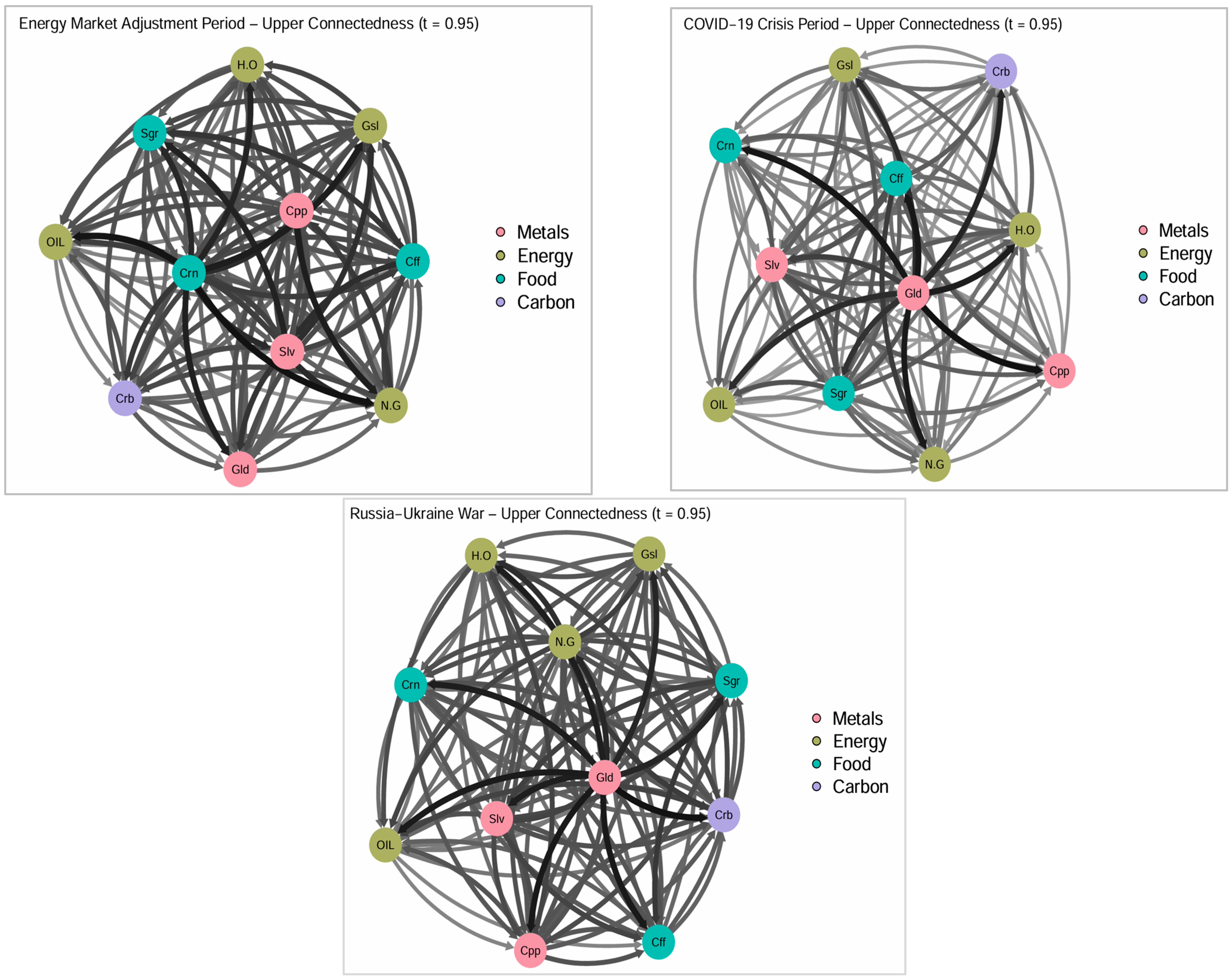
Conversely, the upper-tail network (τ = 0.95) reflects market exuberance and periods of policy-induced optimism, revealing a highly interconnected and complex web of spillovers. In this setting, nearly all commodities engage in bidirectional volatility transmission. Gold assumes a central position in the network, exhibiting strong connections with copper, silver, and carbon, which may indicate its role as an inflation hedge and a focal point of portfolio reallocation during periods of optimism. This is supported by [12,35], who document gold’s dominant systemic role during bull markets and inflationary shocks. Natural gas and carbon also feature prominently, consistent with their growing systemic importance in the global energy transition and climate finance narratives. Interestingly, food commodities such as sugar, coffee, and corn transition from peripheral roles to active contributors and recipients of volatility spillovers, likely driven by inflationary pressures and increased linkages through biofuel markets and commodity-indexed financial instruments. This observation complements [3,20], who report more substantial upper-tail spillovers in agricultural commodity markets during inflationary and conflict-driven market conditions. In this regime, the prevalence of two-way spillovers is consistent with synchronized repricing during rallies, when inflation expectations, inventory constraints, and speculative positioning transmit volatility across sectors.

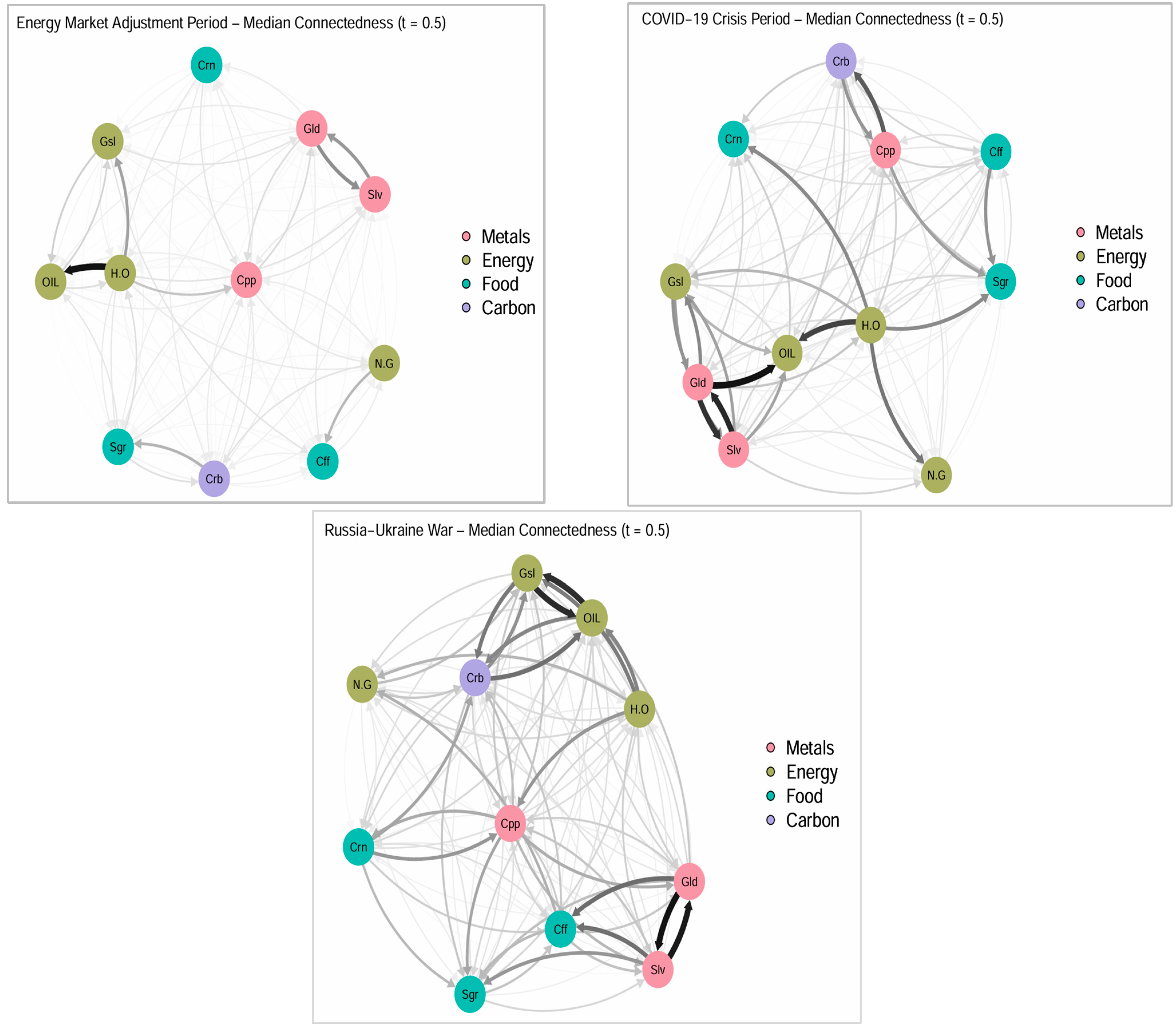
Figure 5 further illustrates median connectedness (τ = 0.5) across major crisis periods, offering additional insights into how systemic interdependencies among commodities and carbon assets manifest under typical market conditions.

Figure 5 indicates meaningful differences in systemic relationships under median (typical) conditions across significant crisis periods. During the energy market adjustment period, the network appears relatively sparse, characterized by a few concentrated volatility spillovers. Notably, there are strong bidirectional linkages within the metals sector, particularly between gold and silver, indicating their co-movement as financial hedges and industrial inputs. Within the energy complex, heating oil serves as a conduit for crude oil volatility, indicating its pivotal role among refined petroleum products. This finding aligns with those of [47,48], who document the transmission of intra-sector risk and the central role of refined energy products in volatility networks. The remainder of the network remains weakly connected, suggesting relatively limited systemic risk under average market conditions.

In contrast, during the COVID-19 crisis, the network structure became significantly more interconnected, reflecting widespread contagion across commodity classes. Energy-related assets, specifically crude oil, heating oil, and natural gas, emerge as key transmitters of volatility, driven by unprecedented demand shocks and extreme price collapses. Gold continues to play a central role in the transmission of systemic risk, with strong spillovers to both silver and crude oil, consistent with its historical function as a safe-haven asset in periods of heightened macroeconomic uncertainty. Additionally, carbon markets gain prominence during this period, indicating the increasing relevance of climate-related financial risk in shaping market dynamics. These findings align with those of [10,13,22], who demonstrate the intensification of spillovers from both carbon and precious metals during COVID-induced financial dislocation. Carbon’s increased connectivity during this episode is consistent with a policy-and-compliance channel in which changing expectations about emissions costs and transition policy interact with energy-price dislocations, thereby strengthening cross-sector volatility transmission.

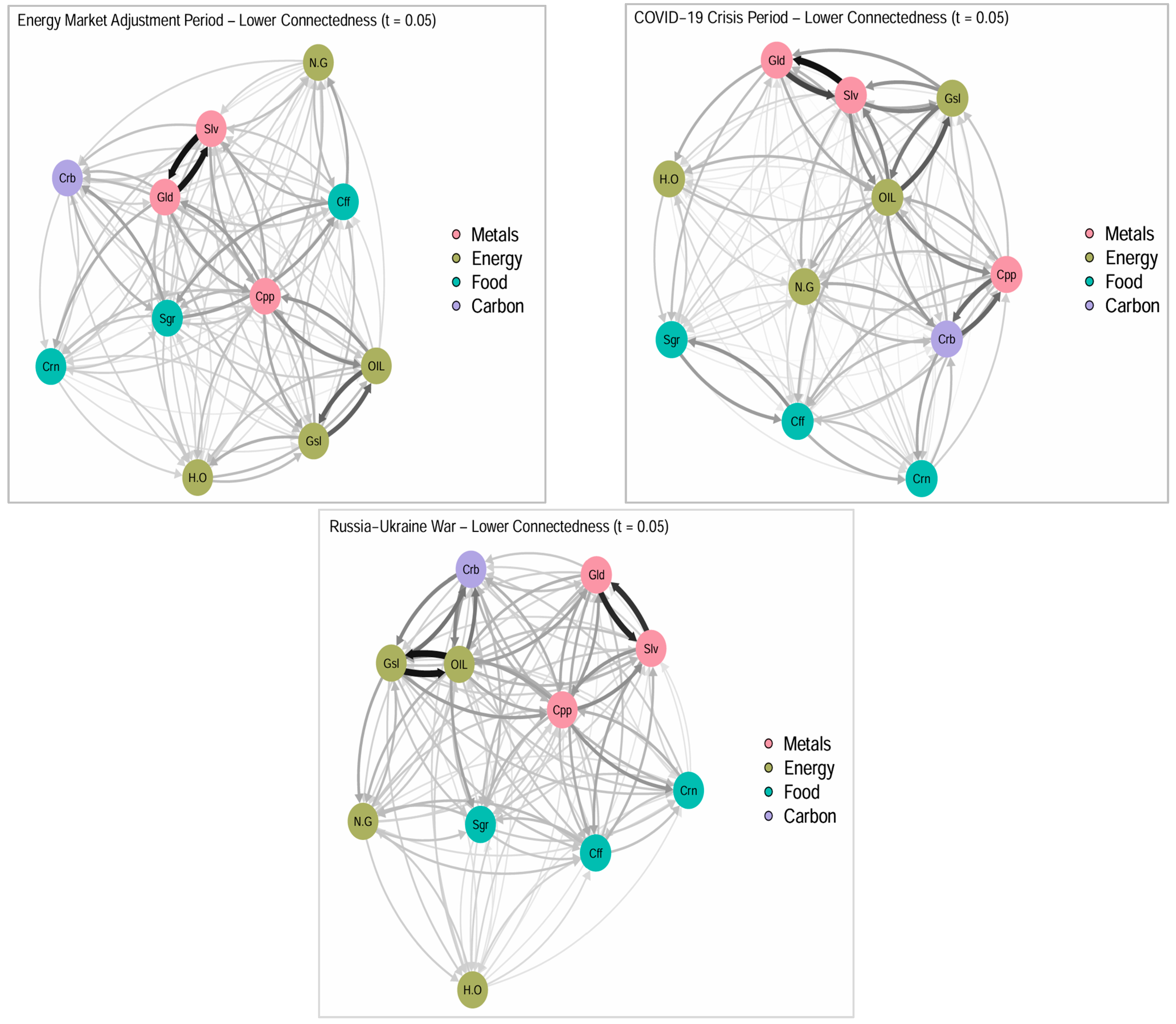
During the Russia–Ukraine war, the median connectedness network becomes even more intensified, particularly within the energy sector. A strong bidirectional linkage forms between gasoline and crude oil, indicative of acute geopolitical stress, supply chain disturbances, and evolving global trade patterns. Carbon markets emerge as a key bridging node, connecting energy assets with both the metals and agricultural sectors, which reflects their expanding role in transmitting climate policy signals and emissions-based adjustments across financial markets. The pairwise connection between gold and silver remains a stable subnetwork, reinforcing their joint importance as crisis hedging instruments. Meanwhile, food commodities and industrial metals occupy more peripheral positions within the network, indicating that their volatility is driven more by external spillovers than by endogenous influences. This aligns with the findings of [3,8], who note that geopolitical crises intensify systemic spillovers, particularly in energy and carbon markets. Figure 6 extends this analysis by presenting the average directional connectedness networks at the lower quantile (τ = 0.05) for each of the three crisis periods.

Under downside risk conditions, all three crisis periods exhibit elevated levels of systemic connectedness, though with distinct structural characteristics. During the energy market adjustment period, volatility spillovers are primarily concentrated within asset classes. Strong intra-sector linkages emerge between gold and silver, as well as between gasoline and crude oil, indicating internal transmission mechanisms within the metals and energy sectors amid uncertainty related to global energy transitions. Such sector-specific transmission patterns align with the findings of [47,49], who demonstrate that sector-bound spillovers intensify during systemic shocks.

In the COVID-19 crisis, the downside network reflects broader systemic distress, characterized by intensified bilateral spillovers across key assets. Gold, silver, gasoline, and crude oil constitute the core of this contagion structure, indicating widespread financial panic and oil-market dislocations. Notably, copper and carbon markets also emerge as significant transmitters of volatility, highlighting their heightened responsiveness to macroeconomic shocks and evolving climate-related regulatory pressures. This result aligns with evidence from [7,11], who underscore the expanding role of industrial metals and carbon in transmitting crisis-induced tail risk.

In contrast, the Russia–Ukraine war generates the most intricate and densely connected downside network. Carbon markets become deeply embedded within the spillover loop linking energy and metals, functioning as a systemic conduit amid overlapping geopolitical tensions and environmental uncertainty. This aligns with [25,50], who demonstrate that carbon markets have become a pivotal node linking sectors during crises. Figure 7 illustrates the upper-tail (τ = 0.95) volatility spillover networks across the three significant crisis periods.

Across all three periods, the network structures exhibit higher density, indicating heightened systemic transmission during episodes of sharp volatility surges triggered by inflationary pressures or geopolitical disruptions. During the energy market adjustment period, crude oil, corn, and silver emerged as prominent drivers, indicating their central role in commodity price rallies and inflation-related repricing. This finding supports the results of [4,51], who report similar roles for silver and food commodities as upper-tail transmitters during inflationary shocks. In contrast, during the COVID-19 crisis, gold assumes a dominant position within the network, transmitting volatility to a broad spectrum of assets, including copper, natural gas, and corn. This pattern highlights gold’s strategic function during periods of global liquidity shocks and heightened demand for safe-haven assets. Similar conclusions are drawn by [15,16,28], who demonstrate gold’s systemic prominence in high-volatility scenarios.

The Russia–Ukraine war period is characterized by a highly dense and interconnected structure, in which nearly all assets exhibit significant two-way volatility spillovers. Gold, crude oil, and copper stand out as central hubs, reflecting deep systemic integration and amplified contagion potential. Carbon markets are consistently well-connected across all scenarios, reinforcing their growing systemic relevance amid regulatory uncertainty and the global energy transition. These results align with those of [10,30], who document widespread volatility comovements and heightened tail-risk transmission across commodities during the war. The persistently high connectedness observed in the upper quantile regime illustrates the synchronized and interdependent behavior of commodity and carbon markets during periods of extreme positive volatility driven by global crises.

Table 3. Net Connectedness across Tail Quantiles Before and During Major Crisis Events.

Net	Copper	Silver	Gold	OIL WTI	Heating Oil	Natural Gas	Gasoline	Sugar	Coffee	Corn	Carbon
Before EMA-low	12.81799	2.7334	15.2498	−4.81705	−5.66267	−5.19872	−4.66828	−1.54374	−0.70678	−7.3563	−0.84765
During EMA-low	10.88998	9.793337	11.13501	−2.41501	−6.6137	−9.01776	2.630707	−0.35207	−2.66645	−7.48097	−5.90307
Before EMA-up	−1.09317	−19.0507	−12.9296	−20.4231	−10.0787	18.52333	−3.17964	10.22555	14.75695	4.043603	19.20552
During EMA-up	8.267327	13.51924	−6.55797	−28.202	−6.20624	−7.93527	4.380971	−2.52846	8.382696	25.79162	−8.91189
Before COVID-low	−3.52112	8.12147	10.95900	0.19495	−2.60126	5.20727	−1.90446	−3.56270	−1.63532	−7.20001	−4.05782
During COVID-low	−0.25420	15.00936	3.77470	20.30853	−7.21613	−9.35830	1.83650	−11.29019	−5.03169	−10.62970	2.85113
Before COVID-up	6.40186	5.62451	−8.54858	−18.13888	9.60838	−14.06822	−28.26729	11.14595	6.79927	36.36153	−6.91853
During COVID-up	−26.14717	17.72153	53.26634	−28.25764	7.97213	−8.88798	−5.44719	14.41523	14.38898	−14.48222	−24.54200
Before RUW-low	0.65761	13.97307	−0.17290	28.06110	−14.84858	−8.11472	10.13612	−12.80975	−12.11646	−9.83905	5.07354
During RUW-low	9.51646	2.02408	2.84193	12.52370	−10.34115	−7.17682	12.13487	−9.97101	−5.50865	−10.21035	4.16694
Before RUW-up	31.84376	−16.40955	61.87447	−39.51326	−6.48791	−15.27243	8.27889	−5.26763	−6.59263	15.60113	−28.05484
During RUW-up	2.62927	4.77936	29.91887	−20.34822	−8.20207	8.18850	−6.12886	−0.45845	−2.94712	−8.04056	0.60928

Note: This table reports the average net directional connectedness values for each asset before and during three major global events: (i) the Energy Market Adjustment (EMA, 2015–2016), (ii) the COVID-19 pandemic (2020), and (iii) the Russia–Ukraine war (RUW, 2022 onward). Net connectedness is computed at the lower (5%) and upper (95%) quantiles using a Quantile-on-Quantile Connectedness framework. Positive values indicate net transmitters of shocks, while negative values indicate net receivers.

provides a quantitative complement to the visual network results in Figure 4, Figure 5, Figure 6 and Figure 7 by summarizing how net connectedness shifts across tail quantiles and crisis periods.

The results demonstrate apparent shifts in the systemic roles of key assets across quantiles and crises. During the Energy Adjustment, Copper and Silver maintained their status as net transmitters in both tails, while Gold and WTI Oil remained net receivers. However, Gold’s influence weakened notably at the upper tail. A sharp contrast emerges during the COVID-19 crisis, where Copper shifted from a moderate net transmitter to a significant net receiver in the upper quantile (from +6.40 to −26.15), indicating increased exposure to systemic risk. Meanwhile, Gold and Carbon exhibited substantial increases in upper-tail net connectedness, indicating their role as safe-haven and regulatory-sensitive assets, respectively. The Russia–Ukraine war period discloses further asymmetries. WTI Oil and Natural Gas, closely linked to geopolitical shocks, intensified their net transmitting roles, especially in the lower quantile. Conversely, assets like Carbon and Gold reversed their positions from pre-war periods, becoming strong net receivers, particularly in the upper tail. This reversal suggests a defensive reallocation by investors during prolonged conflict. The quantification from Table 3 confirms that connectedness dynamics are highly crisis- and quantile-specific, with certain assets (e.g., Gold, Carbon, Natural Gas) exhibiting substantial regime shifts in their systemic influence across time and risk levels.

To move beyond visual inspection and quantify how the connectedness structure changes across episodes, we construct an additional summary of crisis-induced structural shifts.

Table 4. Crisis-induced Structural Shifts in Median and Tail Connectedness.

Event	Regime	Mean TCI (Before)	Mean TCI (During)	ΔTCI	Top Net Transmitters (Before)	Top Net Transmitters (During)
EMA 2015–2016	(τ = 0.05)	58.41	58.70	0.29	Gold, Copper	Gold, Copper, Silver
EMA 2015–2016	(τ = 0.50)	44.98	43.56	−1.42	Natural Gas	Heating Oil, Carbon, Natural Gas
EMA 2015–2016	(τ = 0.95)	99.36	98.93	−0.43	Carbon, Natural Gas	Corn, Silver, Coffee
COVID-19 2020	(τ = 0.05)	57.74	62.93	5.19	Gold, Silver	Crude Oil, Silver, Gold
COVID-19 2020	(τ = 0.50)	42.54	56.53	13.99	Natural Gas	Heating Oil, Gold, Silver
COVID-19 2020	(τ = 0.95)	99.05	99.69	0.65	Corn, Sugar	Gold, Silver, Sugar
RUW 2022–2025	(τ = 0.05)	64.61	63.22	−1.39	Crude Oil, Silver	Crude Oil, Gasoline, Copper
RUW 2022–2025	(τ = 0.50)	59.49	48.76	−10.73	Gold, Heating Oil	Heating Oil, Corn, Silver
RUW 2022–2025	(τ = 0.95)	98.67	98.34	−0.33	Gold, Copper	Gold, Natural Gas, Silver

Note: This table summarizes crisis-induced structural shifts in volatility connectedness across three quantile regimes (lower tail τ = 0.05, median τ = 0.50, and upper tail τ = 0.95). For each event, Mean TCI (Before) and Mean TCI (During) report the average Total Connectedness Index over the pre-event benchmark window and the event window, respectively, and ΔTCI is the difference (During minus Before). Top net transmitters list the three assets with the highest average net connectedness in each window within the specified quantile regime.

reports, for each event window and quantile regime, the average TCI before and during the episode and the corresponding change (ΔTCI). It also summarizes system reallocation through the number of assets that switch from net transmitters to net receivers (or vice versa) and lists the top net transmitters in each window. This compact quantification provides a consistent benchmark for comparing how the network reorganizes across the Energy Market Adjustment, COVID-19, and the Russia–Ukraine war.

Table 4 highlights clear episode- and regime-dependent structural shifts in connectedness. The COVID-19 episode is associated with the strongest system-wide amplification under typical conditions, with the median TCI rising markedly (ΔTCI = 13.99), and with a re-ranking of net transmitters toward the energy complex and precious metals, consistent with large demand disruptions and synchronized rebalancing across commodities. In contrast, the Russia–Ukraine war period shows a decline in median connectedness (ΔTCI = −10.73), indicating a more selective transmission structure under typical conditions despite persistent geopolitical stress, while downside spillovers remain concentrated in energy-related hubs such as crude oil and gasoline. Across regimes, the top-transmitter lists indicate systematic role switching: refined energy products and natural gas become more influential transmitters during event windows, while carbon and agricultural commodities enter the transmitter set primarily in specific regimes, supporting the view that crisis spillovers are driven by value-chain linkages, inventory constraints, and policy-sensitive repricing rather than uniform co-movement across all markets.

5.3. Quantile-Quantile Connectedness

We investigate the state-dependent nature of volatility spillovers across commodities and carbon assets by employing a Quantile-on-Quantile Connectedness approach. We follow the methodology of [47] by examining the interaction between different quantiles of shocks and responses. Figure 8 presents the TCI heatmap across quantile combinations, highlighting asymmetries in spillover intensity under varying market conditions (Volatility inputs are obtained from univariate GARCH (1,1) models (normal innovations) fitted to weekly log-returns for each series, and the resulting conditional standard deviations are used as the QVAR system variables. Quantile connectedness is estimated using a rolling-window QVAR with lag order p = 1, and bias-corrected connectedness measures are used. For tail-specific dynamics, we set τ = (0.05,0.05), (0.50,0.50), and (0.95,0.95) with forecast horizon F = 10. For the quantile-on-quantile maps, we use a 5 × 5 grid of thresholds, τ ∈ {0.05, 0.275, 0.50, 0.725, 0.95}, for shocks and responses, and set F = 20).

Figure 8 indicates an apparent asymmetry in volatility spillovers across quantile combinations. Volatility connectedness intensifies markedly as we move toward the upper-right corner of the matrix, i.e., when both the shock and response quantiles are high (τ = 0.95), with the TCI peaking at 99.5. This suggests that extreme upside volatility events (e.g., sharp rallies or speculative surges) are associated with more substantial system-wide spillovers. Conversely, spillovers are relatively muted in the central region (e.g., τ = 0.5, 0.5) and the lower-left corner, indicating that median or downside market conditions generate less systemic contagion. The results highlight nonlinear and state-dependent dynamics, with connectedness being most pronounced during extreme bullish or high-volatility episodes. These findings are consistent with [16,23], who report more substantial volatility spillovers in the upper quantiles, particularly during episodes of market exuberance and crises. Additionally, refs. [15,47] emphasize that spillovers are more severe in the tails than at the median, highlighting the inadequacy of mean-based connectedness models in capturing systemic risk. Economically, stronger connectedness when both shock and response states are extreme is consistent with tighter funding and inventory constraints and more synchronized positioning, which can increase cross-market volatility transmission when markets are jointly in high-stress or high-exuberance states.

These findings also carry significant implications for tail-risk management frameworks. In particular, the identification of extreme spillover intensities at the tails of the distribution (τ = 0.05 and τ = 0.95) offers practical insights for models based on Value-at-Risk (VaR) and Conditional VaR (CVaR). For instance, the elevated connectedness under upper-tail conditions (τ = 0.95) highlights the systemic importance of commodities like Natural Gas and Heating Oil during speculative rallies or inflationary surges, guiding risk managers to allocate capital buffers accordingly. Conversely, the lower-tail spillovers captured at τ = 0.05 indicate the need for portfolio-level stress testing and dynamic hedging strategies focused on assets such as Crude Oil and Corn, which emerge as major transmitters during downturns. By indicating directional dependencies among extreme-quantile interactions, the Quantile-on-Quantile approach enhances the precision of VaR/CVaR-based risk assessments and supports the design of more robust, tail-sensitive investment strategies.

5.4. NET Quantile-on-Quantile Risk Transmission

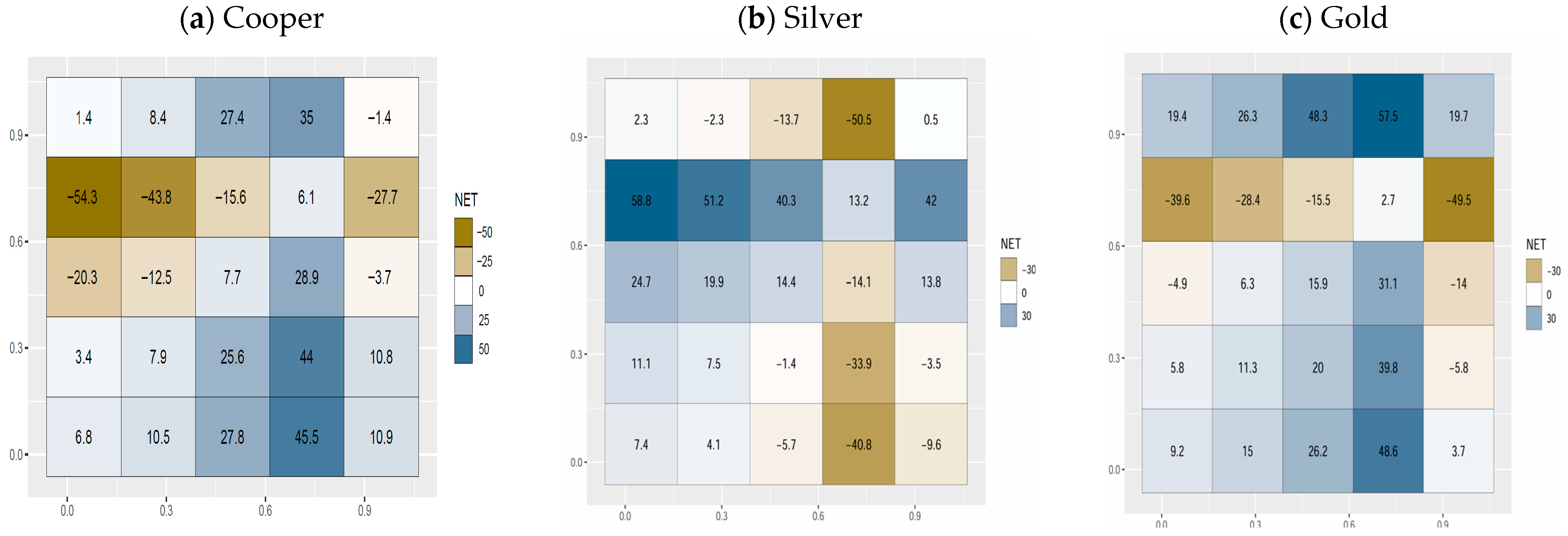
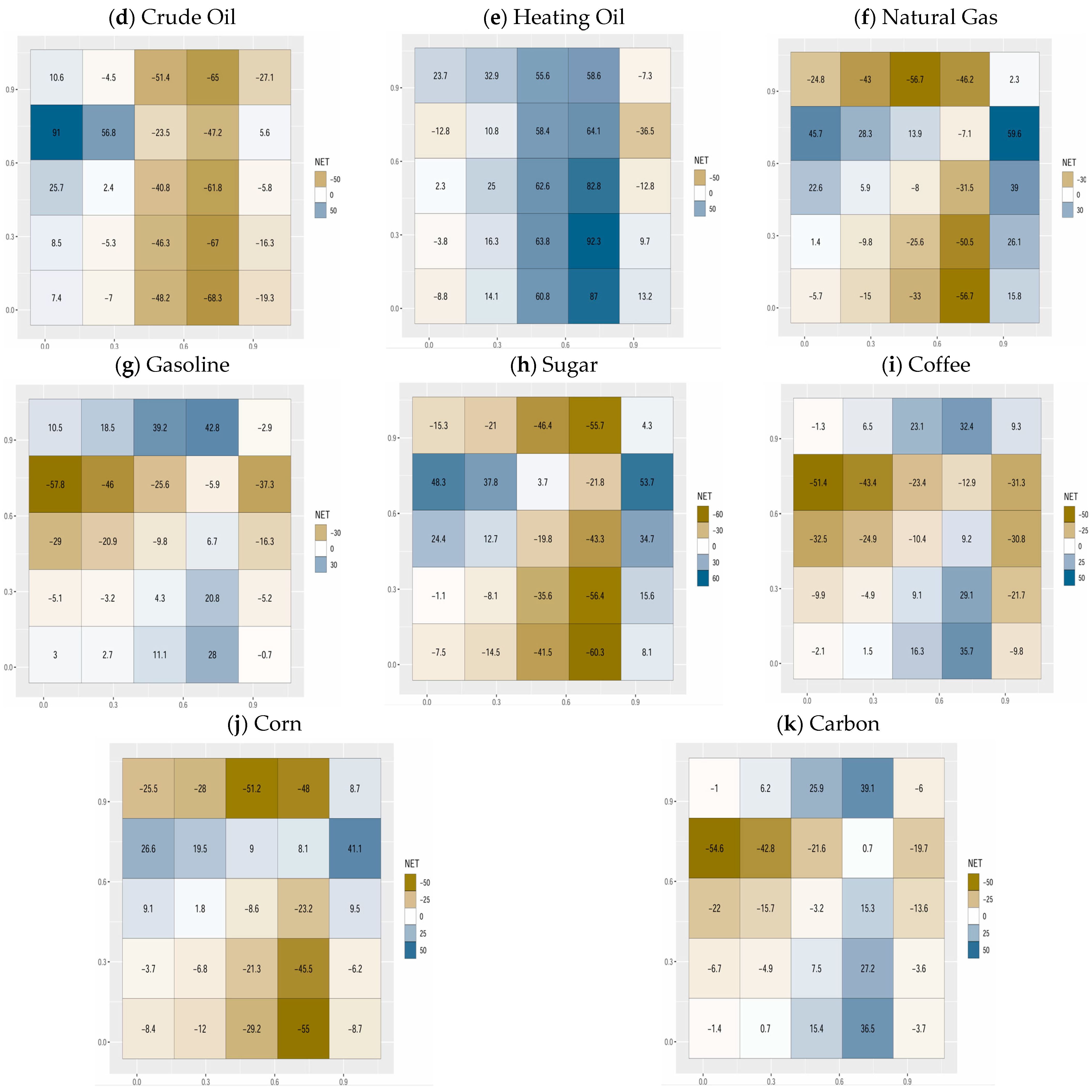
Figure 9 provides a comprehensive visualization of the average net directional connectedness across commodities and carbon assets, evaluated over all quantile combinations of shocks (rows) and responses (columns).

The results expose substantial asymmetries and regime dependencies in volatility transmission dynamics across the commodity spectrum. Copper and Silver exhibit dual roles, acting as net transmitters during bearish or moderately favorable regimes, but switching to receivers under stress, indicating their sensitivity to both economic cycles and flight-to-quality dynamics. This behavioral asymmetry aligns with findings by [5,11], who report regime-switching patterns for industrial and precious metals in response to quantile-based shocks. Gold, consistent with its safe-haven narrative, absorbs systemic shocks under normal conditions but becomes a key transmitter during extreme tail volatility, particularly in risk-off markets. This aligns with [28,35], who document gold’s transformation into a central transmitter under financial and geopolitical distress. Among energy commodities, Crude Oil and Natural Gas show contrasting spillover behaviors. Crude Oil aggressively transmits volatility during transitional phases but absorbs spillovers during high-risk episodes, reflecting its centrality in the propagation of macro-financial stress. This asymmetric behavior is corroborated by [39,50], who highlight oil’s shifting role as transmitter or absorber depending on tail-event magnitudes. In contrast, Natural Gas generally behaves as a receiver except when extreme shocks drive upper-quantile responses, at which point it switches to a net transmitter, highlighting its idiosyncratic sensitivity to tail risks. These results align with findings by [8], who report that natural gas is a conditional risk transmitter during geopolitical crises. Heating Oil emerges as a robust systemic transmitter across most regimes, reinforcing its critical role in energy contagion channels. Similar conclusions are drawn by [23], who identify Heating Oil as a dominant risk hub in bullish market regimes. Meanwhile, Gasoline exhibits a regime-dependent pattern, absorbing volatility during stress but transmitting volatility during extreme bullish responses, possibly linked to demand-side macroeconomic indicators. The agricultural commodities Sugar, Coffee, and corn exhibit predominantly net-receiver profiles, particularly under mid- to upper-quantile shocks, indicating vulnerability to broader market disturbances. However, each shows occasional transmitter behavior under selective conditions (e.g., upper response tails), suggesting that their systemic influence is episodic rather than persistent. This finding is consistent with those of [19,20], who demonstrate that agricultural commodities often absorb risk, except in high-stress or inflation-driven scenarios. Finally, Carbon Emissions Futures mostly absorb spillovers, especially under elevated volatility. However, they can act as mild transmitters under low-shock, high-response states, highlighting their evolving role within the clean energy–finance nexus. These dynamics align with [7,46], who emphasize carbon’s growing yet conditional role in transmitting risk under ESG and climate-policy uncertainty.

5.5. Direct vs. Reverse Connectedness Dynamics

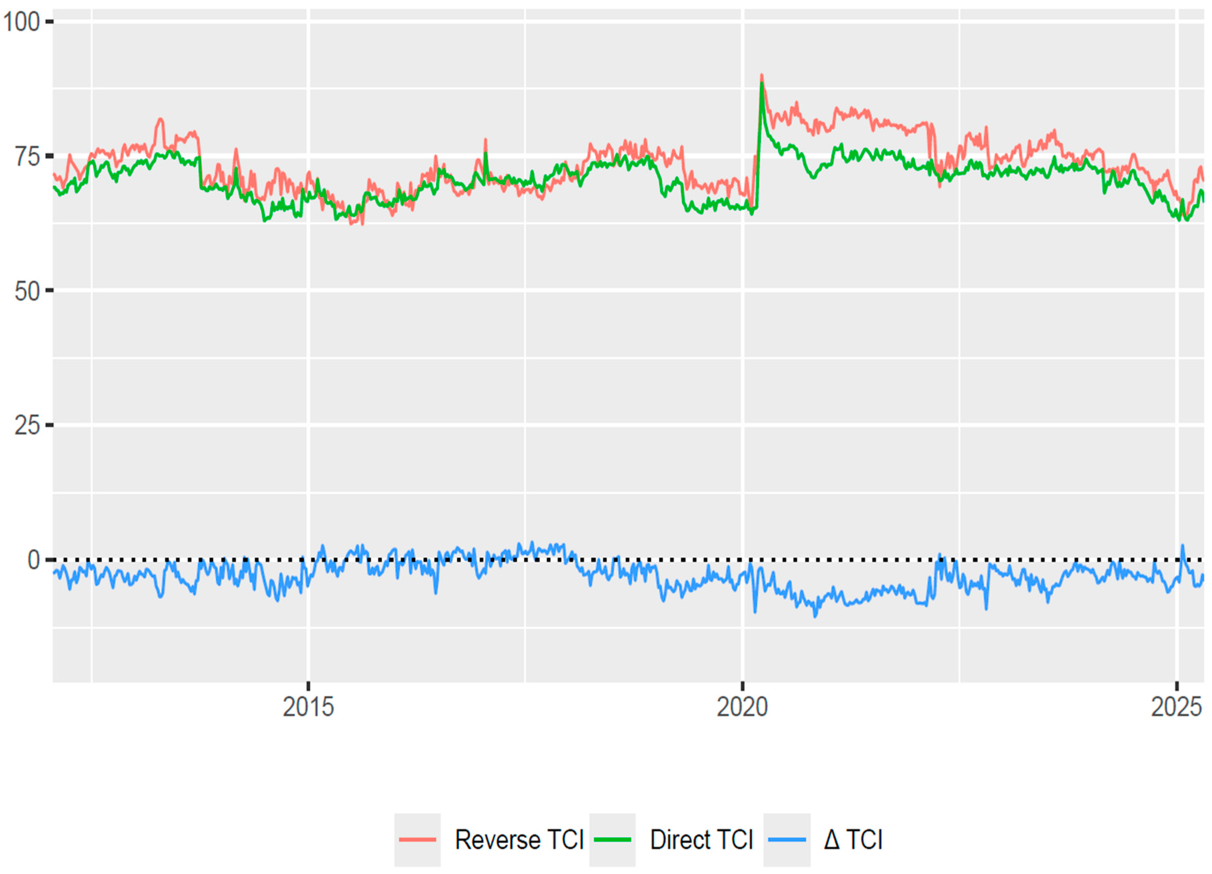
Figure 10 depicts the dynamic evolution of Total Connectedness asymmetry in the global commodity system by contrasting Direct TCI (green line), Reverse TCI (red line), and their difference, ΔTCI (blue line).

Periods with large positive ΔTCI values indicate forward-dominant spillover transmission, suggesting that shocks propagate more strongly in the system’s standard direction. Conversely, negative ΔTCI values indicate reverse-dominant dynamics, where the system absorbs more volatility than it emits. Notably, significant shifts occur around early 2020, coinciding with the COVID-19 shock, during which ΔTCI spikes sharply, indicating intensified asymmetries in volatility transmission. Additional fluctuations in ΔTCI, such as the reversal around 2022, may be attributed to events like the Russia–Ukraine War, energy price shocks, and tightening climate policy measures, which differentially impacted energy, metal, and agricultural commodities. Across the full sample, the persistently nonzero ΔTCI indicates a structurally asymmetric architecture of commodity connectivity, driven by regime shifts and external macro-financial shocks.

5.6. Dynamic Connectedness

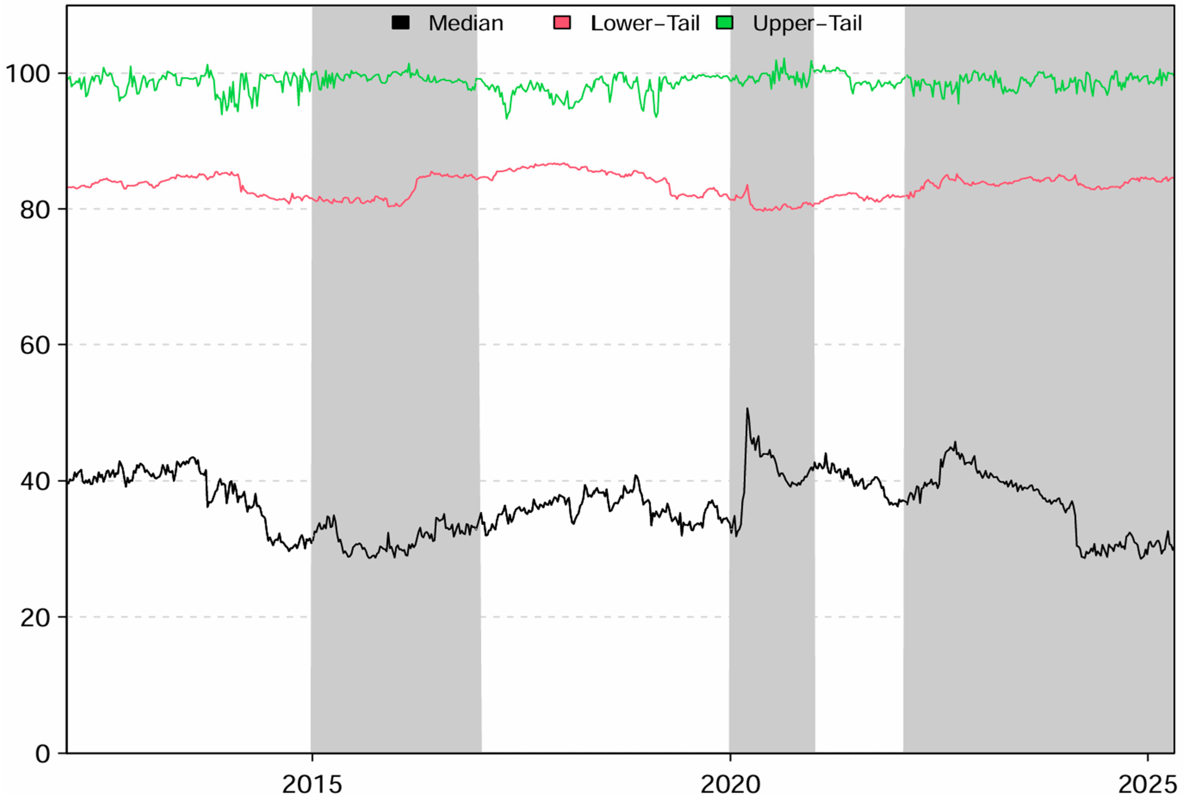
Figure 11 illustrates the time-varying Total Connectedness Index (TCI) across three quantiles, upper-tail (τ = 0.95), lower-tail (τ = 0.05), and median (τ = 0.50), capturing the dynamics of volatility spillovers under different market conditions.

The upper-tail connectedness (green line) remains remarkably stable and persistently high, consistently hovering around 100% throughout the sample. This pattern indicates a high degree of co-movement among commodities in response to extreme positive shocks, such as speculative rallies or synchronized optimism, underscoring systemic fragility during periods of bullishness. Refs. [16,49] report similar upper-tail dominance in systemic spillovers, particularly during commodity price rallies and episodes of capital reallocation. In contrast, the lower-tail connectedness (red line) represents the strength of downside spillovers and shows a more variable but persistently elevated trend. It exhibits notable spikes during major crises, particularly around the COVID-19 outbreak in early 2020 and the onset of the Russia–Ukraine conflict in 2022. These surges reflect heightened vulnerability and contagion during episodes of economic distress and geopolitical tension, where adverse shocks propagate more forcefully across commodity markets. Comparable results are reported by [8,10], who find that total and tail-based spillovers surged during both crises.

The median connectedness (black line) captures average volatility transmission and generally exhibits lower levels during stable periods (e.g., 2016–2018). However, it increases significantly during stress events, peaking above 65 during the early stages of the pandemic and again following the escalation of the Russia–Ukraine war. This behavior confirms that volatility linkages remain subdued under normal conditions but intensify rapidly in response to systemic shocks. These trends are supported by [15,50], who demonstrate that mean-based connectedness rises significantly during crises, albeit weaker than tail-based metrics. Shaded regions mark key global disruptions. During the 2015–2016 energy market adjustment, the median TCI declined, while the lower tail remained elevated, revealing underlying fragility despite a calmer average outlook. The COVID-19 crisis led to an unprecedented spike in connectedness across all quantiles, driven by sharp demand-side shocks and financial uncertainty. Similarly, the Russia–Ukraine conflict sustained elevated spillovers, particularly in the lower quantile, highlighting persistent geopolitical risk transmission across the global commodity system.

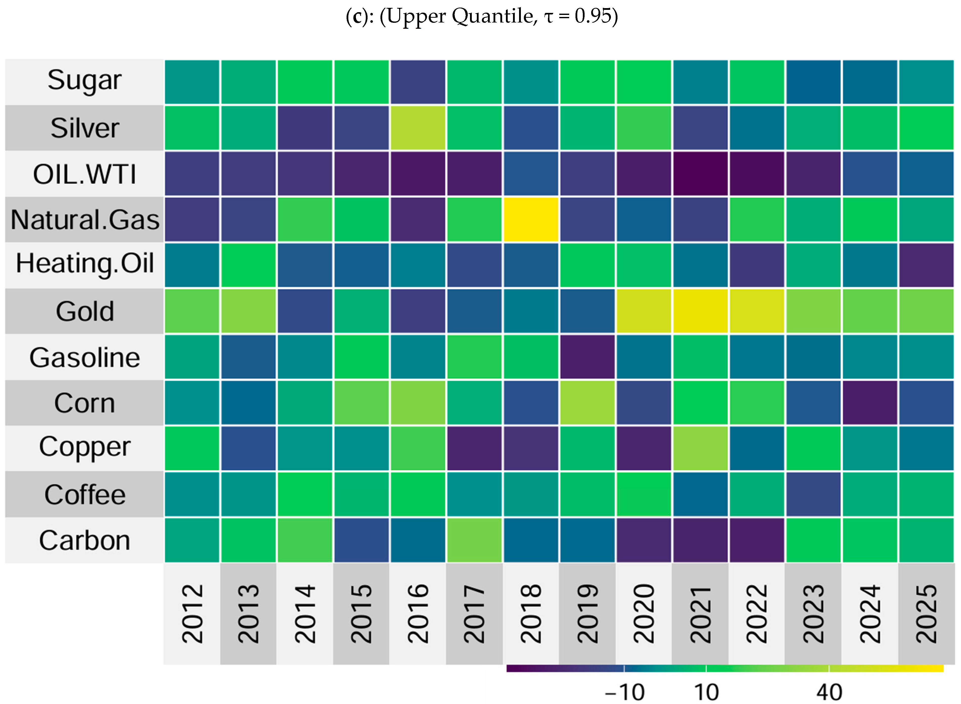
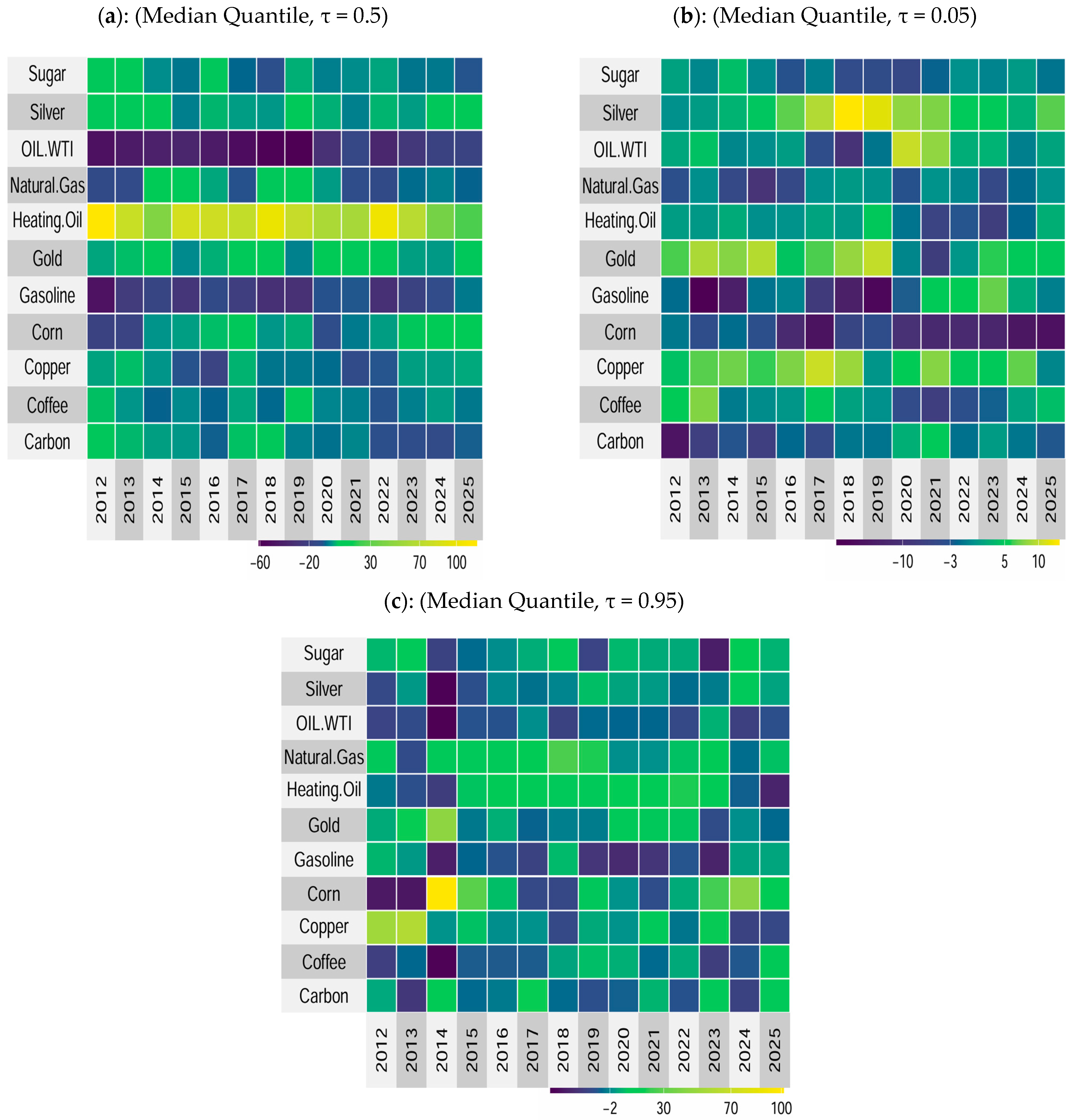
Figure 12 visualizes the annual average net directional connectedness for each asset across quantiles for commodity and carbon assets. A lighter color (yellow-green) indicates strong transmission, while darker hues (blue-purple) denote shock absorption.

At the median quantile (Figure 12a), which reflects typical market conditions, Heating Oil consistently appears to be a dominant net transmitter of volatility for most of the sample period (2012–2021). This persistent role suggests its importance in influencing cross-commodity volatility, likely due to its strong ties to industrial demand and energy markets. This finding aligns with [23], who highlight the systemic centrality of Heating Oil in commodity networks under stable and favorable conditions. Gold, Silver, and Carbon Futures also show positive and stable net connectedness, indicating their contribution to systemic risk transmission. This may be attributed to their use as hedging instruments and their exposure to policy-sensitive sectors such as environmental, social, and governance (ESG) markets. Consistent with [7,48], these assets emerge as key transmitters because of their links to green finance and risk sentiment.

On the other hand, Crude Oil (WTI) frequently functions as a net receiver of volatility, particularly during periods such as the oil price adjustments between 2014 and 2016 and the COVID-19 crisis from 2020 to 2021. This finding suggests that WTI prices are more responsive to external shocks than acting as sources of systemic volatility under average conditions. Similar asymmetries are documented by [39,50], who note that oil shifts between transmitter and receiver roles depending on the market state and the shock origin. Natural Gas, Gasoline, and Sugar similarly exhibit negative or near-zero connectedness, reflecting limited influence on broader market dynamics. From 2022 onward, as geopolitical risks associated with the Russia–Ukraine conflict escalated, the connectedness structure became more evenly distributed. Notably, commodities such as corn and Coffee assume greater transmission roles, reflecting increased cross-market sensitivity driven by inflationary pressures, supply chain disruptions, and the growing link between energy and agriculture. These dynamics align with the findings of [3,25], who demonstrate that food and soft commodities gained influence amid geopolitical conflicts and inflation shocks.

In the lower-tail quantile (Figure 12b), which captures extreme downside market conditions, the structure of systemic transmission undergoes a significant shift. Crude Oil (WTI) emerges as a key net transmitter of volatility, especially during the period from 2020 to 2023. This aligns with the post-COVID recovery phase and the intensification of the Russia–Ukraine conflict, both of which affected global supply chains and energy security. These observations corroborate [2,20], who document Crude Oil’s dominance in transmitting downside shocks during extreme geopolitical and supply-side events. Gold also plays a significant role in transmission during earlier years (2012–2016) and again after 2021, reaffirming its reputation as a safe-haven asset whose volatility affects other markets during financial instability and monetary policy shifts. Gasoline and Silver increase in importance as downside transmitters, likely due to their links to demand shocks and macroeconomic uncertainty. This finding is consistent with [8,11], who find intensified spillovers from silver and energy fuels under left-tail stress. In contrast, Natural Gas and Heating Oil exhibit limited transmission in the lower tail, indicating that their volatility spillovers are more constrained under stress conditions. Among agricultural commodities, Corn and Sugar are consistent net receivers, particularly since 2015, highlighting their vulnerability to external shocks, including currency volatility, weather events, and fluctuations in global demand. This mirrors the findings of [40,46], who emphasize the sensitivity of grains and softs to exogenous tail risks and climate disruptions. Carbon Futures transitioned from passive receivers in the early period (2012–2013) to moderate transmitters after 2017, especially in 2021 and 2023. This change reflects the growing influence of emissions markets, climate-related financial risks, and environmental regulations on commodity market dynamics. This is supported by [22,47], who note that carbon assets increasingly act as systemic transmitters under ESG and climate policy-driven volatility.

At the upper tail quantile (Figure 12c), which reflects extreme positive-volatility events, Natural Gas consistently acts as a strong net transmitter. This role is especially evident in the periods 2014 to 2015, 2017 to 2018, and from 2022 onward. These episodes coincide with heightened energy demand, weather-related supply issues, and geopolitical developments. This aligns with [2,11], who identify Natural Gas as a key source of upper-tail volatility under inflationary and policy-driven conditions. Gold also demonstrates substantial positive connectedness from 2020 to 2023, indicating its systemic influence during inflationary periods and episodes of monetary policy uncertainty, particularly around the COVID-19 crisis and global capital reallocations. Carbon futures have emerged as net transmitters since 2022, suggesting the increasing influence of energy transition policies and climate risks on market spillovers. Similar insights are provided by [7,22,46], who document the increasing prominence of carbon assets in upper-tail risk-transmission networks. In contrast, Crude Oil (WTI) consistently serves as a net receiver of volatility during upper-tail events between 2014 and 2023. This indicates that oil absorbs rather than spreads volatility during bullish conditions, possibly due to its anchoring role in energy markets. Carbon also experiences periods of net receiver behavior (e.g., in 2015, 2020, and 2022), indicating sensitivity to external shocks without feeding systemic volatility. Furthermore, corn and copper have shifted from being minor transmitters to net receivers in recent years, especially after 2021. This reflects their increased exposure to global commodity shocks during a period of changing market structure. These observations align with those of [47,51], who highlight how previously peripheral commodities can become more shock-sensitive and systemic in response to climate transition and geopolitical risks.

From a financial perspective, the findings emphasize that systemic volatility spillovers vary across market regimes. Assets such as Gold and Natural Gas become especially influential during upper-tail conditions and require close monitoring in risk management and portfolio design. From an economic standpoint, the results indicate that the importance of different commodities changes over time, influenced by developments in monetary policy, energy security, and climate regulation. The growing influence of Carbon markets in recent years illustrates the integration of environmental concerns into financial risk transmission channels. This transformation of the carbon-finance nexus is also highlighted in the works of [5,7], who emphasize carbon’s evolving role as both a policy-sensitive instrument and a systemic financial node.

5.7. Robustness Check

5.7.1. Alternative Volatility Measures

To ensure the robustness of the connectedness results, this subsection implements an alternative measure of volatility based on realized volatility (RV) computed from squared daily returns aggregated at the weekly frequency. Unlike GARCH-based conditional volatilities, RV captures actual market fluctuations without relying on parametric assumptions, making it particularly useful for validating findings under model-free settings.

As shown in Figure A1, the dynamic Total Connectedness Index (TCI) estimated from realized volatility remains persistently elevated in the upper tail of the distribution. In contrast, the lower tail and median quantiles exhibit pronounced spikes during key crisis periods, such as the COVID-19 pandemic and the Russia–Ukraine war. This pattern closely mirrors the main findings in Figure 11, which uses GARCH-based volatility, reinforcing the robustness of the tail-dependent connectedness structure across both volatility measures. As shown in Figure A2, the heatmaps of pairwise net directional connectedness under realized volatility confirm the broad patterns established using GARCH-based volatility (Figure 12). Specifically, Heating Oil and Copper remain prominent net transmitters across all quantiles, while Natural Gas and Gold consistently act as net receivers, especially in the lower tail. These spillover patterns persist across both crisis periods and calm phases, indicating that the dominant roles of key commodities are robust to the underlying volatility measure. Minor differences in magnitude do appear, particularly for Gasoline and Silver, yet the directional structure and temporal dynamics remain largely consistent. This reinforces the credibility of the main findings and confirms that the observed tail-risk spillovers are not driven by volatility model specification.

As an additional robustness check, we re-estimate the median connectedness dynamics using alternative volatility filters that account for heavy tails and asymmetric responses in commodity markets. Specifically, I replace the baseline Gaussian sGARCH (1,1) volatility series with Student-t sGARCH (1,1) and Student-t GJR-GARCH (1,1) volatilities, and then recompute the rolling QVAR-based median TCI using the same connectedness settings.

Figure A3 shows that the three TCI series move closely together over time and identify the same episode-level surges, particularly during the COVID-19 period and the Russia–Ukraine war. This consistency indicates that the main conclusions about systemic volatility co-movement and crisis amplification are not driven by the Gaussian volatility assumption, and remain stable when allowing for fat-tailed shocks and leverage-type asymmetries in the volatility extraction step.

5.7.2. Controlling for Common Global Drivers

To assess whether the estimated volatility connectedness is driven primarily by common global risk factors rather than cross-market transmission within the commodity-carbon system, we conduct an additional robustness exercise that partials out major macro-financial drivers. Specifically, we consider three widely used global proxies: the U.S. Dollar Index (DXY), the U.S. 10-year Treasury yield (US10Y), and the CBOE Volatility Index (VIX). These variables capture, respectively, broad dollar strength and global liquidity conditions, benchmark interest-rate dynamics, and global risk aversion.

In this robustness check, we used DXY, US10Y, and VIX at a weekly frequency and aligned them with the weekly GARCH-based volatility series. We then residualize each commodity and carbon volatility series by regressing it on the standardized driver set (DXY, US10Y, VIX), and retain the residual component as a “driver-adjusted” volatility measure. Next, we re-estimate the median QVAR-based using the residualized volatilities and compare it with the baseline median TCI computed from the original volatilities. This design allows us to evaluate whether the time variation in connectedness persists after filtering out the influence of common global drivers. Figure A4 compares the baseline median TCI with the driver-adjusted median TCI.

Figure A4 indicates that the overall dynamics remain qualitatively similar, indicating that the connectedness patterns are not solely a reflection of global risk conditions. At the same time, differences in levels across certain episodes suggest that global drivers contribute to the magnitude of connectedness, particularly during major stress periods, but do not eliminate the underlying state-dependent interdependence captured by the QQ-QVAR framework.

5.7.3. Robustness to the Carbon Market Proxy

To address concerns that a single carbon futures series may not fully represent the heterogeneity of global emissions trading systems, we conduct an additional robustness check using an alternative benchmark from the European Union Emissions Trading System (EU ETS). Specifically, we replace the baseline carbon series with European Union Allowance (EUA) Yearly Futures (EU ETS) and re-estimate the connectedness measures while keeping the rest of the system unchanged. This robustness design assesses whether the commodity–carbon spillover dynamics are sensitive to the specific carbon proxy used. This robustness design assesses whether the commodity-carbon spillover dynamics are sensitive to the specific carbon proxy used. We then recompute the volatility inputs using the same univariate GARCH-based volatility extraction step and re-estimate the median QVAR connectedness under the same rolling-window configuration, lag order, forecast horizon, and bias-correction settings. Figure A5 compares the time-varying median Total Connectedness Index (TCI) obtained from the baseline carbon proxy against the corresponding TCI obtained using the EUA proxy.

Figure A5 indicates that the median connectedness dynamics are nearly unchanged when carbon is proxied by EU ETS EUA futures. The time variation and the timing of major peaks remain highly consistent across the two specifications, implying that the core connectedness patterns are not driven by idiosyncrasies of a single carbon benchmark. This evidence supports the generalizability of our main conclusions regarding carbon’s integration within the commodity risk transmission network, while acknowledging that cross-ETS heterogeneity remains an important direction for future research, given that comparable long-span data for other ETS markets are available.

5.7.4. Frequency Sensitivity Test

To address concerns that weekly sampling may smooth short-run spillovers and affect connectedness dynamics, we conduct a frequency sensitivity exercise using the same volatility series aggregated to lower frequencies. Starting from the weekly GARCH-based volatility measures, we construct (a) a bi-weekly series by averaging volatility within consecutive two-week blocks and (b) a monthly series by averaging within calendar months. For each frequency, we re-estimate the median QVAR connectedness (τ = 0.50) using the same baseline settings (lag length and forecast horizon), while scaling the rolling-window length proportionally to the sampling interval to preserve a comparable effective time span. We compare the standardized (z-score) median TCI series across frequencies. Figure A6 reports the standardized median TCI for weekly, bi-weekly, and monthly sampling. The co-movement of the three standardized series indicates that the main episode timing and medium-run fluctuations in connectedness are robust to frequency choice, suggesting that weekly sampling does not drive the qualitative dynamics reported in the baseline results.

To strengthen the statistical credibility of the magnitudes of connectedness, we compute 95% moving-block bootstrap confidence intervals for the mean and median of the Total Connectedness Index (TCI; τ = 0.50) using 500 replications and a 10-week block length. The full-sample mean TCI equals 49.77 with a 95% CI of [48.42, 51.33]. Across episodes, the mean TCI is 43.56 [41.95, 44.41] for the Energy Market Adjustment, 56.53 [53.60, 60.88] for COVID-19, and 48.76 [46.47, 50.91] for the Russia–Ukraine war window. Overall, these intervals confirm that the episode differences discussed in the paper are not driven by sampling noise and that the median-regime connectedness levels are estimated with tight uncertainty bands. These results support the reliability of cross-episode comparisons while maintaining the paper’s descriptive interpretation of connectedness.

6. Conclusions and Policy Implications

This study examines the dynamics of systemic volatility transmission across strategic commodity and carbon markets under varying market conditions, utilizing a Quantile-on-Quantile Connectedness framework. Specifically, we addressed three key questions: how volatility is transmitted under normal, adverse, and exuberant regimes; which assets act as net transmitters or receivers of systemic risk; and how these dynamics evolve during significant crises, such as the COVID-19 pandemic and the Russia–Ukraine war. The results indicate asymmetries and nonlinearities in the transmission of risk. Volatility spillovers intensify substantially in both the lower and upper quantiles of the distribution, highlighting distinct contagion structures during distress and exuberance. Under downside shocks (τ = 0.05), systemic risk is amplified, with gold, gasoline, and carbon emerging as the dominant transmitters. In contrast, under upper-tail conditions (τ = 0.95), interconnectedness surges across nearly all assets, with gold, natural gas, and carbon playing central systemic roles. These findings support the classification of carbon not merely as a regulatory or environmental instrument, but as a financialized commodity whose risk dynamics resemble those of traditional market anchors like oil and gold. These results are consistent with a transition environment in which carbon management policies and subsurface decarbonization options (e.g., sequestration and storage pathways) increasingly interact with resource-market risk, strengthening carbon’s potential role as a systemic node.

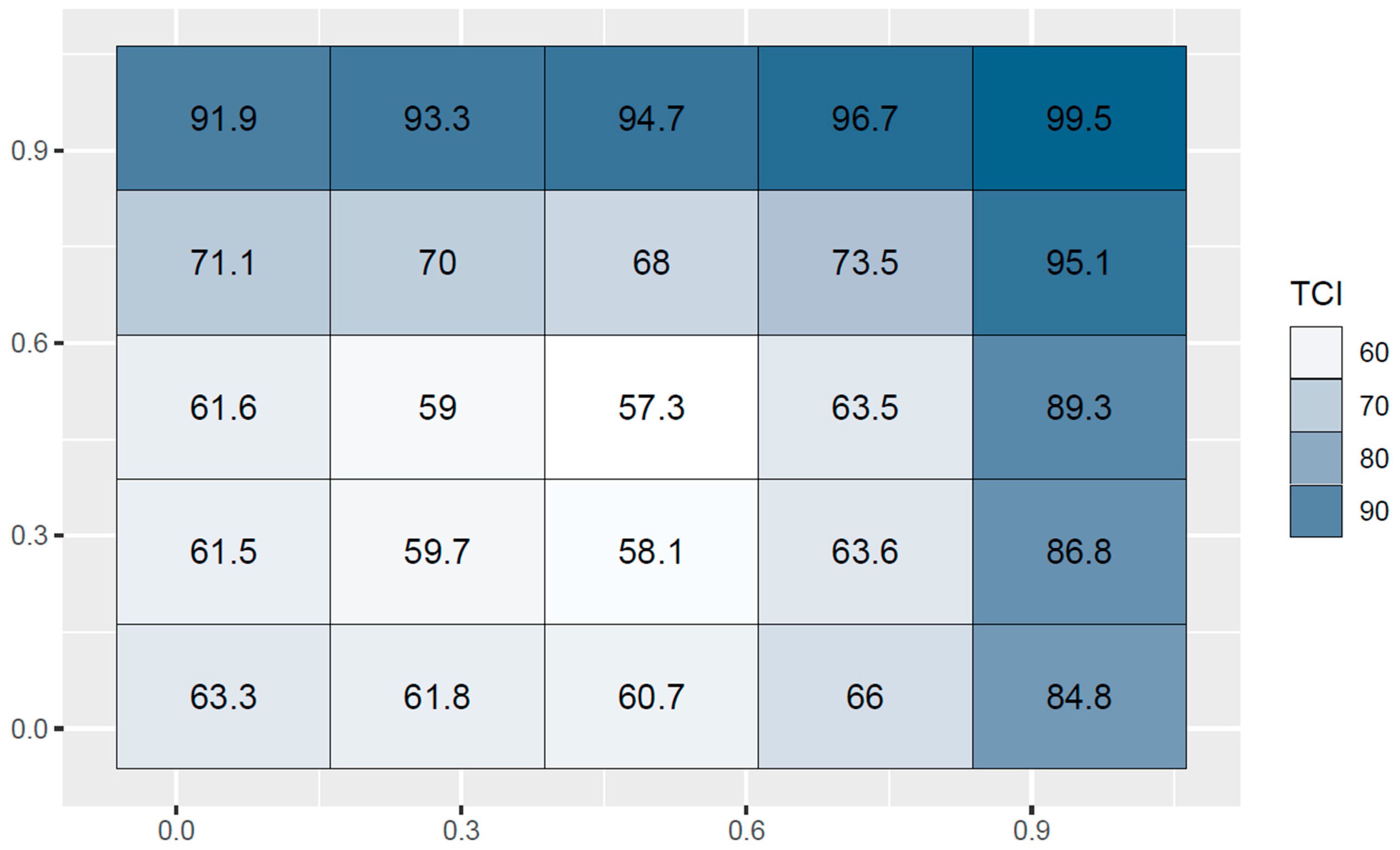
Importantly, the dynamics of transmission varied significantly across crisis episodes. During the 2015–2016 energy market adjustment, spillovers were contained mainly within sectors, reflecting localized transmission. In contrast, the COVID-19 crisis triggered widespread cross-sector contagion, driven by energy dislocations and flight-to-safety behavior centered around gold. The Russia–Ukraine war produced the most densely connected networks, with carbon markets serving as a bridge across energy, metals, and agriculture, indicating their growing role as conduits for geopolitical and climate-related shocks. Furthermore, our net connectedness analysis identifies regime-specific roles of key assets: heating oil, natural gas, and gold frequently act as transmitters during periods of exuberance; crude oil and agricultural commodities tend to absorb shocks, particularly during bearish episodes. The dynamic connectedness metrics confirm that systemic spillovers rise sharply during crises and remain elevated, especially in tail regimes, suggesting persistent vulnerability and interdependence in global commodity-carbon systems.

The results carry direct implications for stakeholders because they identify when connectedness tightens, which markets act as transmission hubs, and when carbon becomes a cross-sector bridge. First, for financial regulators and central banks, we recommend incorporating tail-sensitive connectedness indicators into routine macro-financial surveillance, with particular attention to (a) lower-tail spikes in total connectedness and (b) shifts in net connectedness for key hubs such as gold, refined fuels, natural gas, and carbon. Operationally, this can be implemented as an early-warning “tail connectedness dashboard” that triggers enhanced monitoring when lower- or upper-tail connectedness exceeds its historical percentile thresholds during stress episodes. Second, the evidence that carbon futures can function as a bridge between energy, metals, and agriculture implies that carbon-pricing adjustments and compliance expectations can coincide with broader volatility transmission. Therefore, carbon-market regulators and policy designers should strengthen market-stability safeguards during periods of elevated energy-price volatility, including liquidity-provision mechanisms, transparent margining policies, and monitoring of concentration risk in carbon-derivatives markets. Third, for exchanges and market infrastructure providers, identifying refined energy products and natural gas as recurring transmission channels supports targeted resilience planning. In practice, this implies prioritizing stress scenarios that combine energy supply disruptions with elevated margin calls, and ensuring that trading halts, circuit breakers, and collateral frameworks remain robust when transmission hubs intensify spillovers across markets. Fourth, for institutional risk managers, the results indicate that risk monitoring should not rely on average co-movement measures. Instead, exposure oversight should be state-dependent, with heightened controls when tail connectedness rises and when a previously peripheral asset (notably carbon) becomes more integrated. A practical implication is to complement standard risk reports with regime-specific monitoring of net transmitters and receivers to anticipate where shocks are likely to originate and accumulate. The results highlight that commodity and carbon markets are linked not only through fundamentals but also through state-dependent volatility channels that intensify during major disruptions, indicating the need for integrated oversight of resource markets during periods of heightened macro-financial uncertainty.

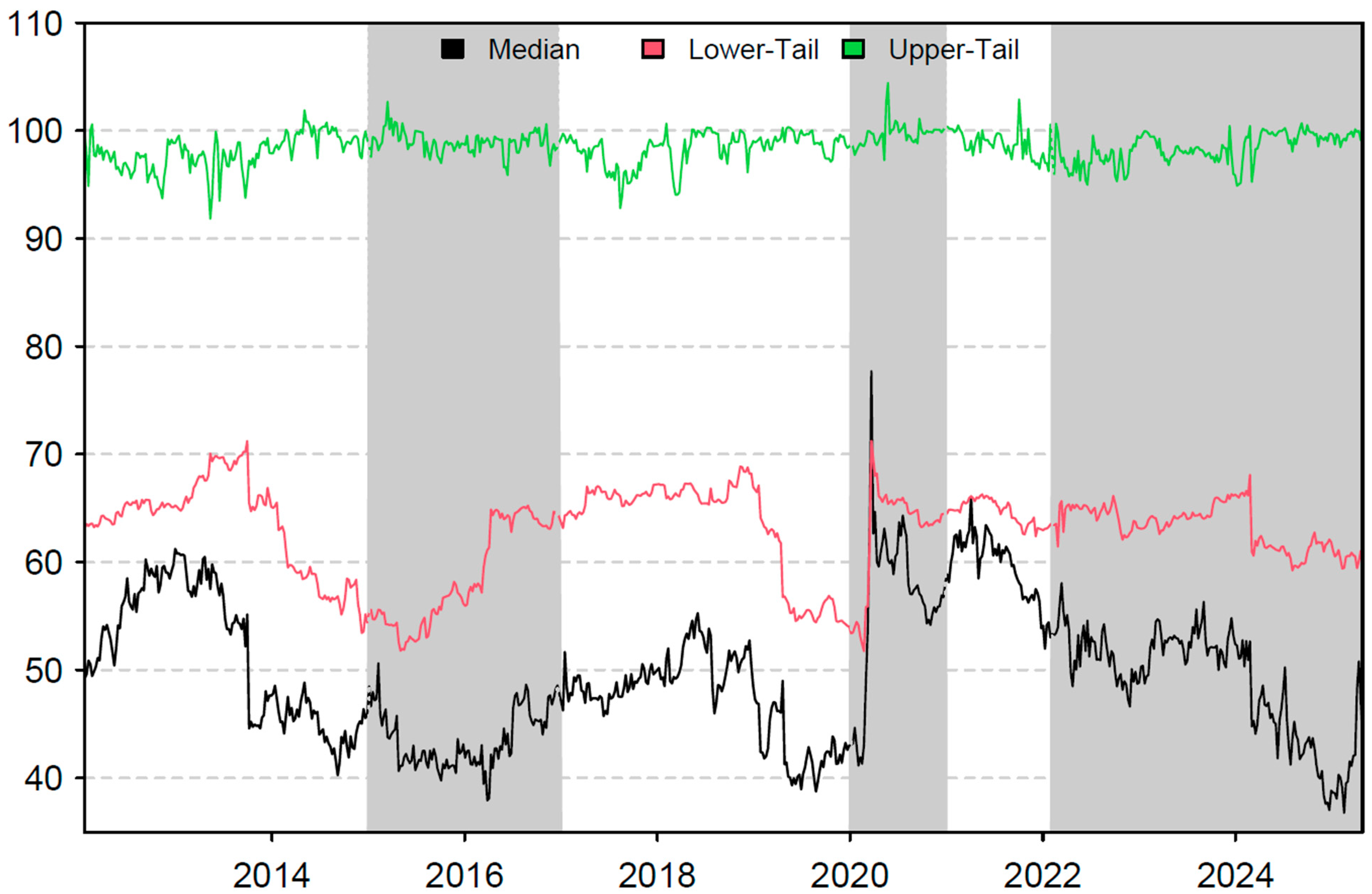
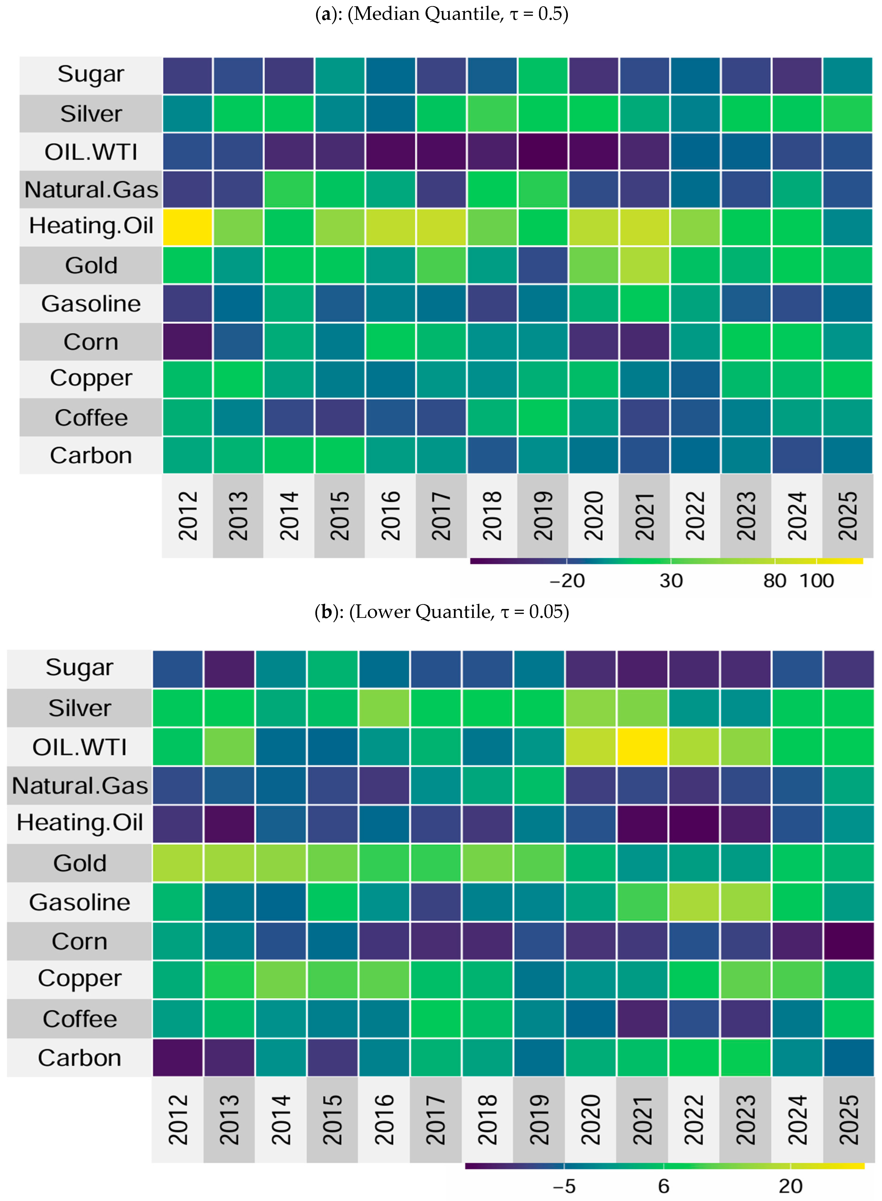
Future research can extend the asset set to include transition-critical commodities such as lithium and cobalt to examine whether transition-sensitive markets become persistent spillover hubs during periods of climate-policy tightening. It can also compare alternative volatility filters, including asymmetric and long-memory specifications, to assess whether the main connectedness rankings are sensitive to the volatility extraction step. Another extension is to incorporate policy and uncertainty indicators, such as climate policy uncertainty and geopolitical risk, to evaluate whether crisis spillovers are primarily market-driven or policy-driven across quantile states. Finally, formal structural break identification, such as Bai–Perron multiple-break tests and Zivot–Andrews unit-root tests with breaks, can be used to date endogenous regime shifts in volatility transmission and to complement the rolling-window evidence.

References

1. Kyriazis, N.; Papadamou, S.; Tzeremes, P.; Corbet, S. Examining spillovers and connectedness among commodities, inflation, and uncertainty: A quantile-VAR framework. Energy Econ. 2024, 133, 107508. [Google Scholar] [CrossRef] [Scilit]
2. Kayani, U.; Hasnaoui, A.; Khan, M.; Zahoor, N.; Nawaz, F. Analyzing fossil fuel commodities’ return spillovers during the Russia and Ukraine crisis in the energy market. Energy Econ. 2024, 135, 107651. [Google Scholar] [CrossRef] [Scilit]
3. Fang, Y.; Shao, Z. The Russia-Ukraine conflict and volatility risk of commodity markets. Finance Res. Lett. 2022, 50, 103264. [Google Scholar] [CrossRef] [Scilit]
4. Zhang, T.; Li, P.F.; Zhou, W.X. Spillover effects between climate policy uncertainty, energy markets, and food markets: A time-frequency analysis. Finance Res. Lett. 2025, 82, 107553. [Google Scholar] [CrossRef] [Scilit]
5. Gao, Y.; Liu, X. Time and frequency spillovers and drivers between rare earth and energy, metals, green, and agricultural markets. N. Am. J. Econ. Finance 2024, 72, 102128. [Google Scholar] [CrossRef] [Scilit]
6. Wang, K.H.; Kan, J.M.; Qiu, L.; Xu, S. Climate policy uncertainty, oil price and agricultural commodity: From quantile and time perspective. Econ. Anal. Policy 2023, 78, 256–272. [Google Scholar] [CrossRef] [Scilit]
7. Qiao, S.; Chang, Y.; Mai, X.X.; Dang, Y.J. Climate policy uncertainty, clean energy and energy metals: A quantile time-frequency spillover study. Energy Econ. 2024, 139, 107919. [Google Scholar] [CrossRef] [Scilit]
8. Naeem, M.A.; Hamouda, F.; Karim, S. Tail risk spillover effects in commodity markets: A comparative study of crisis periods. J. Commod. Mark. 2024, 33, 100370. [Google Scholar] [CrossRef] [Scilit]
9. Chen, Y.; Jiang, W. Time and frequency volatility spillovers among commodities: Evidence from pre and during the Russia-Ukraine war. Port. Econ. J. 2024, 23, 249–273. [Google Scholar] [CrossRef] [Scilit]
10. Cui, J.; Maghyereh, A. Higher-order moment risk connectedness and optimal investment strategies between international oil and commodity futures markets: Insights from the COVID-19 pandemic and Russia-Ukraine conflict. Int. Rev. Financ. Anal. 2023, 86, 102520. [Google Scholar] [CrossRef] [Scilit]
11. Pham, L.; Kamal, J.B. Blessings or curse: How do media climate change concerns affect commodity tail risk spillovers? J. Commod. Mark. 2024, 34, 100407. [Google Scholar] [CrossRef] [Scilit]
12. Li, H.; Li, Y.; Zhang, H. The spillover effects among the traditional energy markets, metal markets and sub-sector clean energy markets. Energy 2023, 275, 127384. [Google Scholar] [CrossRef] [Scilit]
13. Banerjee, A.K. Second-order moment risk connectedness across climate and geopolitical risk and global commodity markets. Econ. Lett. 2024, 235, 111551. [Google Scholar] [CrossRef] [Scilit]
14. Yang, Y.H.; Shao, Y.H.; Zhou, W.X. Contemporaneous and lagged spillovers between agriculture, crude oil, carbon emission allowance, and climate change. Finance Res. Lett. 2025, 71, 106374. [Google Scholar] [CrossRef] [Scilit]
15. Chen, J.; Liang, Z.; Ding, Q.; Liu, Z. Extreme spillovers among fossil energy, clean energy, and metals markets: Evidence from a quantile-based analysis. Energy Econ. 2022, 107, 105880. [Google Scholar] [CrossRef] [Scilit]
16. Iqbal, N.; Bouri, E.; Grebinevych, O.; Roubaud, D. Modelling extreme risk spillovers in the commodity markets around crisis periods including COVID19. Ann. Oper. Res. 2023, 330, 305–334. [Google Scholar] [CrossRef] [Scilit]
17. Tahir, M.U.; Guo, S. Preliminary Investigation of Fracture Behavior during Carbon Dioxide Fracturing of Natural Hydrogen Reservoir with Hard-Core Imperfections. Reserv. Sci. 2026, 2, 34–51. [Google Scholar] [CrossRef] [Scilit]
18. Wu, J.; Ansari, U. From CO2 Sequestration to Hydrogen Storage: Further Utilization of Depleted Gas Reservoirs. Reserv. Sci. 2025, 1, 19–35. [Google Scholar] [CrossRef] [Scilit]
19. Just, M.; Echaust, K. Dynamic spillover transmission in agricultural commodity markets: What has changed after the COVID-19 threat? Econ. Lett. 2022, 217, 110671. [Google Scholar] [CrossRef] [Scilit]
20. Tiwari, A.K.; Abakah, E.J.A.; Adewuyi, A.O.; Lee, C.C. Quantile risk spillovers between energy and agricultural commodity markets: Evidence from pre and during COVID-19 outbreak. Energy Econ. 2022, 113, 106235. [Google Scholar] [CrossRef] [Scilit]
21. Xing, X.; Liu, Y.; Zhu, Y.; Deng, J. The impact of climate policy uncertainty on China’s green energy and non-ferrous metals market co-movement: Evidence from spillover perspectives. J. Environ. Manag. 2024, 367, 121845. [Google Scholar] [CrossRef] [Scilit]
22. Gao, W.; Wei, J.; Zhang, H.; Zhang, H. Does climate policy uncertainty exacerbate extreme risk spillovers between green economy and energy metals? Resour. Policy 2024, 91, 104946. [Google Scholar]
23. Zhang, X.; Yang, X.; He, Q. Multi-scale systemic risk and spillover networks of commodity markets in the bullish and bearish regimes. N. Am. J. Econ. Finance 2022, 62, 101766. [Google Scholar] [CrossRef] [Scilit]
24. Foroni, B.; Morelli, G.; Petrella, L. The network of commodity risk. Energy Syst. 2024, 15, 167–213. [Google Scholar] [CrossRef] [Scilit]
25. Wang, Z.; Zhu, H.; Mi, Y. Multidimensional risk contagions in commodity markets: A multi-layer information networks method. N. Am. J. Econ. Finance 2025, 79, 102457. [Google Scholar] [CrossRef] [Scilit]
26. Hung, N.T. Oil prices and agricultural commodity markets: Evidence from pre and during COVID-19 outbreak. Resour. Policy 2021, 73, 102236. [Google Scholar] [CrossRef] [Scilit]
27. Ren, X.; Xiao, S.; Zhang, W.; Sun, X. Tail risk spillover of commodity futures markets. Account. Finance 2025, 65, 109–141. [Google Scholar] [CrossRef] [Scilit]
28. Kamal, M.M.; Roca, E.; Li, B.; Lin, C.; Reza, R. Price contagion and risk spillover in the global commodities market: COVID-19 pandemic vs. global financial crisis. Resour. Policy 2025, 103, 105553. [Google Scholar] [CrossRef] [Scilit]
29. Lin, B.; Zhang, Z. Extreme spillovers among green finance, energy, and energy metals markets in China: Evidence under the dilemma of energy transition. Renew. Energy 2025, 241, 122403. [Google Scholar] [CrossRef] [Scilit]
30. Biswas, P.; Jain, P.; Maitra, D. Are shocks in the stock markets driven by commodity markets? Evidence from Russia-Ukraine war. J. Commod. Mark. 2024, 34, 100387. [Google Scholar] [CrossRef] [Scilit]
31. Xiao, B.; Yu, H.; Fang, L.; Ding, S. Estimating the connectedness of commodity futures using a network approach. J. Futures Mark. 2020, 40, 598–616. [Google Scholar] [CrossRef] [Scilit]
32. Wu, F.; Zhao, W.L.; Ji, Q.; Zhang, D. Dependency, centrality and dynamic networks for international commodity futures prices. Int. Rev. Econ. Finance 2020, 67, 118–132. [Google Scholar] [CrossRef] [Scilit]
33. Ren, Y.; Tan, A.; Zhu, H.; Zhao, W. Does economic policy uncertainty drive nonlinear risk spillover in the commodity futures market? Int. Rev. Financ. Anal. 2022, 81, 102084. [Google Scholar] [CrossRef] [Scilit]
34. Dahl, R.E.; Oglend, A.; Yahya, M. Dynamics of volatility spillover in commodity markets: Linking crude oil to agriculture. J. Commod. Mark. 2020, 20, 100111. [Google Scholar] [CrossRef] [Scilit]
35. Kang, S.H.; McIver, R.; Yoon, S.M. Dynamic spillover effects among crude oil, precious metal, and agricultural commodity futures markets. Energy Econ. 2017, 62, 19–32. [Google Scholar] [CrossRef] [Scilit]
36. Anwer, Z.; Khan, A.; Naeem, M.A.; Tiwari, A.K. Modelling systemic risk of energy and non-energy commodity markets during the COVID-19 pandemic. Ann. Oper. Res. 2025, 345, 1193–1227. [Google Scholar] [CrossRef] [Scilit]
37. Li, H.; Li, Y.; Guo, L. Extreme risk spillover effect and dynamic linkages between uncertainty and commodity markets: A comparison between China and America. Resour. Policy 2023, 85, 103839. [Google Scholar] [CrossRef] [Scilit]
38. Chen, Y.; Qi, H. COVID-19 pandemic-related news and Chinese commodities futures: Time-frequency connectedness and causality-in-quantiles approaches. Energy 2024, 286, 129610. [Google Scholar] [CrossRef] [Scilit]
39. Zhou, X.; Enilov, M.; Parhi, M. Does oil spin the commodity wheel? Quantile connectedness with a common factor error structure across energy and agricultural markets. Energy Econ. 2024, 132, 107468. [Google Scholar] [CrossRef] [Scilit]
40. Hu, X.; Zhu, B.; Zhang, B.; Zeng, L. Extreme risk spillovers between US and Chinese agricultural futures markets in crises: A dependence-switching copula-CoVaR model. PLoS ONE 2024, 19, e0299237. [Google Scholar] [CrossRef] [Scilit] [PubMed]
41. Liao, X.; Li, W. Research on the tail risk contagion in the international commodity market on the China’s financial market: Based on a network perspective. Kybernetes 2025, 54, 807–831. [Google Scholar] [CrossRef] [Scilit]
42. Adebayo, T.S.; Olanrewaju, V.O. How effective are trade policy and monetary policy in achieving a pathway to sustainable development? Evidence from a wavelet quantile-on-quantile Granger causality analysis. Sustain. Dev. 2025, 33, 861–877. [Google Scholar] [CrossRef] [Scilit]
43. Gabauer, D.; Stenfors, A. Quantile-on-quantile connectedness measures: Evidence from the US treasury yield curve. Finance Res. Lett. 2024, 60, 104852. [Google Scholar] [CrossRef] [Scilit]
44. Jia, S.; Chen, X.; Han, L.; Jin, J. Global climate change and commodity markets: A hedging perspective. J. Futures Mark. 2023, 43, 1393–1422. [Google Scholar] [CrossRef] [Scilit]
45. Nasreen, S.; Tiwari, A.K.; Goodell, J.W.; Tedeschi, M. Asymmetric and frequency-domain spillover effects among industrial metals, precious metals, and energy futures markets. Int. Rev. Econ. Finance 2024, 93, 1556–1592. [Google Scholar] [CrossRef] [Scilit]
46. Zeng, H.; Abedin, M.Z.; Ahmed, A.D.; Lucey, B. Quantile and Time–Frequency Risk Spillover Between Climate Policy Uncertainty and Grains Commodity Markets. J. Futures Mark. 2025, 45, 659–682. [Google Scholar] [CrossRef] [Scilit]
47. Arfaoui, N.; Roubaud, D.; Naeem, M.A. Energy transition metals, clean and dirty energy markets: A quantile-on-quantile risk transmission analysis of market dynamics. Energy Econ. 2025, 143, 108250. [Google Scholar] [CrossRef] [Scilit]
48. Huang, S.; Wang, X.; Ji, Q. How unexpected geopolitical risk affect the nonlinear spillover among energy and metal markets? Energy Econ. 2025, 142, 108143. [Google Scholar] [CrossRef] [Scilit]
49. Zhang, H.; Zhang, Y.; Gao, W.; Li, Y. Extreme quantile spillovers and drivers among clean energy, electricity and energy metals markets. Int. Rev. Financ. Anal. 2023, 86, 102474. [Google Scholar] [CrossRef] [Scilit]
50. Jiang, W.; Chen, Y. Impact of Russia-Ukraine conflict on the time-frequency and quantile connectedness between energy, metal and agricultural markets. Resour. Policy 2024, 88, 104376. [Google Scholar] [CrossRef] [Scilit]
51. Zheng, Q.; Wu, J.; Lin, B. Geopolitical Risk and Extreme Risk Connectedness Among Energy and Other Strategic Commodities: Fresh Sight Using the High-Dimensional CoVaR Model. J. Futures Mark. 2024, 44, 1787–1806. [Google Scholar] [CrossRef] [Scilit]
Figure 1. Pearson Correlation Heatmap.
Resources 15 00053 g001
Figure 2. Quantile ADF Test Results.
Resources 15 00053 g002
Figure 3. Quantile PP Test Results.
Resources 15 00053 g003
Figure 4. Quantile-Based Full Sample Connectedness Networks among Commodities and Carbon Markets. Note: 11 assets, grouped into Metals, Energy, Food, and Carbon Markets, under three quantiles: (a) Median Connectedness (τ = 0.5) reflects average interdependence, (b) Lower-Tail Connectedness (τ = 0.05) captures systemic spillovers during extreme negative shocks, and (c) Upper-Tail Connectedness (τ = 0.95) represents volatility transmission under extreme positive conditions. Arrow thickness and color intensity indicate the strength of spillovers, while node color represents the asset class.
Resources 15 00053 g004
Figure 5. Median Connectedness (τ = 0.5) Across Major Crisis Periods. Note: This figure presents the average directional connectedness networks at the median (τ = 0.5) across three major crisis regimes: the Energy Market Adjustment Period, the COVID-19 Crisis, and the Russia–Ukraine War. The networks reflect systemic spillovers under normal conditions. Thicker and darker arrows represent stronger volatility transmission, while node colors indicate asset class groupings: Metals, Energy, Food, and Carbon Markets.
Resources 15 00053 g005
Figure 6. Lower-Tail Connectedness (τ = 0.05) Networks Across Crisis Periods. Note: This figure presents the average directional connectedness networks at the lower quantile (τ = 0.05) across three major crisis regimes: the Energy Market Adjustment Period, the COVID-19 Crisis, and the Russia–Ukraine War. The networks reflect systemic spillovers under downside risk conditions, such as negative price shocks or financial distress. Thicker and darker arrows represent stronger volatility transmission, while node colors indicate asset class groupings: Metals, Energy, Food, and Carbon Markets.
Resources 15 00053 g006
Figure 7. Quantile-Based Upper-Tail Connectedness Networks (τ = 0.95) across Crisis Periods. Note: This figure presents the upper-tail (τ = 0.95) volatility spillover networks among 11 commodities and carbon assets during three significant events: the Energy Market Adjustment, the COVID-19 Crisis, and the Russia–Ukraine War. Arrow thickness and color intensity represent the strength of average pairwise volatility transmissions under extreme positive shocks. Node colors indicate asset classes: Metals, Energy, Food, and Carbon.
Resources 15 00053 g007
Figure 8. Quantile-on-Quantile Total Connectedness Index (TCI) Heatmap. Note: This figure illustrates the average TCI across all quantile pairs, computed using a rolling-window Quantile Vector Autoregression (QVAR) model applied to GARCH-based volatility series. Each cell shows the mean TCI over time for a specific combination of shock (rows) and response (columns) quantiles. Darker shades indicate stronger volatility spillovers. The heatmap reports the time-averaged Total Connectedness Index (TCI), computed from rolling-window QVAR-based connectedness, using a GARCH (1,1) volatility series. Rows (shock quantiles) and columns (response quantiles) follow a 5 × 5 grid. The QVAR uses lag order p = 1, forecast horizon F = 20, and bias-corrected connectedness measures.
Resources 15 00053 g008
Figure 9. Net Quantile-on-Quantile risk transmission for Commodity and Carbon Assets. Note: Each panel in Figure 6 presents the average net directional connectedness (NET) of a given asset across quantile combinations of shocks (rows) and responses (columns). Positive values indicate the asset acts as a net transmitter of volatility spillovers, while negative values reflect a net receiver. The heatmaps are generated using a Quantile-on-Quantile Connectedness framework, capturing nonlinear and state-contingent spillover patterns under different market conditions: bearish (τ = 0.1), normal (τ = 0.5), and bullish (τ = 0.9). The 11 panels correspond to: (a) Copper, (b) Silver, (c) Gold, (d) Crude Oil, (e) Heating Oil, (f) Natural Gas, (g) Gasoline, (h) Sugar, (i) Coffee, (j) Corn, and (k) Carbon Emissions Futures.
Resources 15 00053 g009aResources 15 00053 g009b
Figure 10. Time-Varying Asymmetry in Total Connectedness. Note: This figure illustrates the time-varying dynamics of Total Connectedness asymmetry across the commodity system. The Direct TCI (green line) captures the average within-group spillovers that arise when shocks originating from an asset affect other assets. In contrast, the Reverse TCI (red line) measures spillovers received by the same asset when other variables are shocked. The ΔTCI (blue line) represents the directional asymmetry (Direct TCI–Reverse TCI). Positive ΔTCI implies dominance of transmitted shocks (net transmitter behavior), whereas negative ΔTCI indicates stronger absorption of volatility (net receiver behavior).
Resources 15 00053 g010
Figure 11. Time-Varying Total Connectedness Index under Median, Lower-Tail, and Upper-Tail Shocks. Note: This figure presents the dynamic Total Connectedness Index (TCI) estimated using the Quantile-on-Quantile VAR (QVAR) approach across the 11-asset volatility network comprising Metals, Energy, Food, and Carbon markets. The TCI is computed at three quantile levels: median (τ = 0.5), lower-tail (τ = 0.05), and upper-tail (τ = 0.95), over a rolling window of 106 weeks. The shaded regions correspond to key global events: the Energy Market Adjustment (2015–2016), the COVID-19 pandemic (2020), and the Russia–Ukraine war (2022 onward).
Resources 15 00053 g011
Figure 12. Annual Net Directional Connectedness Across Quantiles for Commodity Assets. Note: This figure displays heatmaps of annual average net directional connectedness for 11 commodity and carbon assets across three quantiles: (a) Median quantile (τ = 0.5), (b) Upper quantile (τ = 0.95), (c) Lower quantile (τ = 0.05). The connectedness measures are estimated using a QVAR framework applied to GARCH-based volatility series. Each cell’s color represents the average net connectedness for a given asset-year combination, where warmer colors (yellow-green) denote stronger net transmitters of volatility and cooler colors (blue-purple) indicate stronger net receivers.
Resources 15 00053 g012aResources 15 00053 g012b