Abstract
Flow regulation and water quality maintenance are considered ecosystem services, as they provide environmental benefits with a measurable economic value to society. Distributed or semi-distributed hydrological models can help identify where land use decisions yield the greatest economic and environmental returns related to water resources. For these reasons, this study integrated simulations performed with the SWAT (Soil and Water Assessment Tool) model under varying land use conditions, aiming to balance potential benefits with the loss of ecosystem services. Among the tested parameters, those associated with surface runoff showed the highest sensitivity in simulating streamflow for the Jundiaí River Basin. Based on the statistical indicators R2, Nash–Sutcliffe efficiency (NS), and Percent Bias (PBIAS), the SWAT model demonstrated a reliable performance in replicating observed streamflows on a monthly scale, even with limited spatially distributed input data. Scenario 2, which involved converting 15% of pasture/agricultural land into forest, yielded the most favorable hydrological outcomes by increasing soil water infiltration and aquifer recharge while reducing surface runoff and sediment yield. These findings highlight the value of reforestation and land use planning as effective strategies for improving watershed hydrological performance and ensuring long-term water sustainability.
1. Introduction
The southeast region of Brazil—particularly the state of São Paulo—is highly affected by extreme hydrological events, such as floods, inundations, and severe droughts. This is due to its dense population, limited availability of water resources (only 6% of the national total), and high water demand for industrial, agricultural, irrigation, hydroelectric, and public supply purposes [1,2].
The imbalance between water availability and demand for urban and economic uses in São Paulo, especially in the São Paulo Metropolitan Region, is a growing concern. The situation is exacerbated by the lack of water regulation infrastructure in most rivers, which leaves supply systems highly vulnerable—particularly during prolonged and severe droughts [3]. Additionally, most municipalities do not treat their sewage and discharge untreated effluents into stormwater drainage systems, which flow through urban rivers, leading to downstream water quality degradation and posing risks to public supply [4].
Between 2012 and 2016, the São Paulo region experienced one of the most severe droughts recorded in the past 60 years due to a prolonged lack of rainfall. Combined with poor water distribution planning and irregular or unplanned urban land use, the scarcity of rainfall led to a serious water crisis and a drastic reduction in water availability from key supply systems [5,6].
The most critical conditions are found in the São Paulo Metropolitan Region, located in the Alto Tietê Basin, where water availability is just 128.79 m3 per capita per year [4]. The water sources in this basin are insufficient to supply the metropolis, necessitating water transfers from the Atibaia River and further stressing downstream basins. The Jundiaí River Basin is part of this system and is also affected by the urban–industrial expansion of Greater São Paulo. Water demand in the Jundiaí Basin has already exceeded local availability, requiring the diversion of water from the Atibaia River for public supply [7,8]. Given the complexity of water governance in the São Paulo Metropolitan Region and the growing impacts of land use change and climate change, the region must prepare to avoid or mitigate consequences for public health, safety, and the economy.
The reduction in water infiltration capacity caused by urban growth and development leads to a loss of permeable area [9,10], triggering negative environmental impacts that affect landscapes, the local climate, and human well-being [11,12]. While increased vegetation may lead to higher evapotranspiration and a reduced average streamflow [13], the presence of forests also enhances rainfall infiltration, increases aquifer recharge, and contributes to flow regulation throughout the year—especially by maintaining base flows during dry periods, which supports ecosystem services dependent on water availability [14]. Furthermore, native forests play a key role in controlling erosion and sediment input, influencing the physical–chemical characteristics of water bodies [12]. Thus, streamflow regulation can be considered an ecosystem service with real economic value, derived from sustainable land use practices.
Hydrological modeling enables the identification of land use decisions that either favor or hinder sustainable watershed management and allows for the prediction of climate change impacts on regional water balances. Therefore, this study integrates simulations performed with the SWAT (Soil and Water Assessment Tool) hydrological model under different land use scenarios, weighing the trade-offs between environmental service gains and losses.
The SWAT (Soil and Water Assessment Tool) model was originally developed in the United States by the USDA-ARS, with default parameters based on the climatic, geological, hydrological, and pedological conditions typical of that country [15]. For this reason, its application in watersheds in other regions, such as Brazil, requires significant adaptations. These adaptations include the parameterization of local soil types, adjustments to climate data, the definition of region-specific land management practices, and, above all, careful calibration based on regional observational data. In this context, applying SWAT to new watersheds, especially those in tropical environments or areas with distinct land use and land cover patterns, constitutes a relevant methodological contribution.
The SWAT model stands out for its wide-scale use and can be applied in watersheds where the goal is to assess the quantitative aspects of runoff, erosion processes, sediment and nutrient losses from agricultural areas, and water quality, as well as to evaluate the hydrological behavior of sites subject to changes in land use and land cover [15,16].
Recent advances in hydrological modeling have integrated artificial intelligence techniques to improve runoff forecasting and error correction in conceptual models. Wang et al. evaluated the performance of several data preprocessing methods combined with Gated Recurrent Unit (GRU) neural networks for forecasting monthly runoff time series [17]. The results indicated that the appropriate choice of preprocessing significantly enhanced the model’s predictive capability, with direct implications for water resource monitoring and management.
In another study, Wenchuan et al. proposed an error correction methodology based on deep learning to improve the accuracy of conceptual rainfall-runoff models [18]. This approach integrated deep learning techniques to adjust the model’s systematic biases, resulting in significant improvements in water balance simulation and runoff forecasting ability. These advances highlight the growing importance of combining traditional hydrological modeling with artificial intelligence to address complex challenges in watershed management.
Our main objective is to simulate hydrological variables and estimate the effects of forest restoration in the Jundiaí River Basin, with the aim of providing decision support tools for sustainable water management.
2. Materials and Methods
SWAT is processed through a GIS interface—ArcSWAT—using tabular data and spatial information in its simulation. The calibration and validation of the model are carried out in the SwatCup program.
The steps for running the model are presented in the methodological flowchart, which consists of the following seven different stages (Figure 1): acquisition of the database; data input into ArcSWAT; execution of the data to perform the model simulation; sensitivity analysis, which is processed in SwatCup; calibration and validation of the hydrological model, both also processed in SwatCup; and finally, the creation of scenarios with different land use and land cover, which will be performed in ArcGIS.
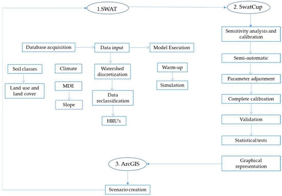
Figure 1.
Methodological flowchart.
2.1. Study Area and Data Availability
The Jundiaí River Basin is part of Water Resources Management Unit 5—Piracicaba, Capivari, and Jundiaí (UGRHI/PCJ), with all three rivers being direct tributaries of the Tietê River. The basin, illustrated in Figure 2, has a drainage area of approximately 1114 km2 and encompasses the following eleven municipalities in the state of São Paulo: Atibaia, Cabreúva, Campo Limpo Paulista, Indaiatuba, Itu, Itupeva, Jarinu, Jundiaí, Mairiporã, Salto, and Várzea Paulista.
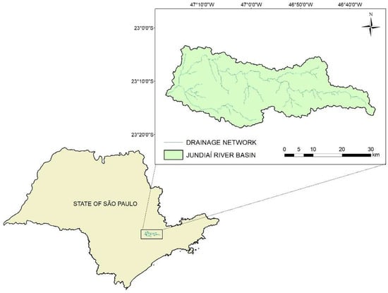
Figure 2.
Location of the Jundiaí River Basin.
The Jundiaí River Basin presents a critical water availability scenario and a highly delicate water balance, relying on the transposition of 1.2 m3/s from the Atibaia River to meet existing water rights [19]. According to 2018 IBGE census data, the basin region has a population of approximately 1.5 million inhabitants, with 95% residing in urban areas and only 5% in rural zones. Jundiaí and Indaiatuba are the most populous municipalities. This urban–rural imbalance is reflected in the local economy, where industry and services dominate economic activity.
The climate in the Jundiaí River Basin is classified as high-altitude tropical (Cwa) under the Köppen system (1936), with hot and rainy summers and mild, relatively dry winters. In terms of land use and land cover, pasture dominates the landscape [20]. Soils are generally low in fertility, which favors reforestation (e.g., eucalyptus plantations) and the cultivation of temperate fruit crops such as strawberries, peaches, and grapes [21].
The core process of hydrosedimentological modeling in SWAT is water balance. Climatic parameters are, therefore, of critical importance, as they influence every stage of this process. Six conventional rain gauge stations provided daily precipitation data from 1973 to 2019, sourced from the Hydrological Information System (HIDROWEB) maintained by the Brazilian National Water Agency (ANA). Additionally, four automatic weather stations supplied by the National Institute of Meteorology (INMET) were used, as listed in Table 1.

Table 1.
Rainfall and climate stations used to obtain historical time series and statistical climate data for the Jundiaí River Basin.
SWAT uses the WXGEN weather generator model [24] to fill gaps in daily meteorological time series and generate missing data. The four automatic weather stations provide daily data on temperature, relative humidity, wind speed, and solar radiation [23]. These climatological inputs are processed through the weather generator and subjected to statistical analysis, enabling the model to simulate the hydrological cycle within the basin [15,25].
Streamflow data were obtained from one streamflow gauging station, as shown in Table 2. Figure 3A displays the spatial distribution of weather, streamflow, and rainfall stations across the Jundiaí River Basin.
Table 2.
Streamflow gauging station used to obtain data on discharge.
Table 2.
Streamflow gauging station used to obtain data on discharge.
| Order | Code | Name | Latitude | Longitude | Drainage Area (km2) | Variable |
|---|---|---|---|---|---|---|
| 1 | 4D-021 | Itaicá | −23.107 | −47.179 | 795 | flow |
Source: Brazilian National Water Agency ANA [26].

Figure 3.
Input data for the SWAT model: (A) digital elevation model and stations (data available from the USGS, SRTM); (B) soil classes (map data from Forestry Institute of the State of São Paulo, according to Rossi 2017 [27]); and (C) land use (map data from MapBiomas 2024).
The land use and land cover maps used in this study were derived from the MapBiomas project (MAPBIOMAS, 2024). As shown in Figure 3C, the classification includes Forest Formation (FRSE), Silviculture (EUCA), Wetlands (WETF), Pasture (PAST), Sugarcane (SUGR), Agriculture/Pasture (AGRL), Urban Area (URBN), Non-Vegetated Areas (URLD), Rocky Outcrops (TIMO), Water Bodies (WATR), Soybeans (SOYB), Other Temporary Crops (AGRC), Coffee (COFF), Citrus (ORAN), and Other Permanent Crops (AGRR).
The soil classes used in the model (Figure 3B) were based on maps from the São Paulo State Forestry Institute and Embrapa, following Santos et al. [28] and Rossi et al. [27]. The main soil types are Red-Yellow Argisol (PVA), Red Latosol (PV), Haplic Cambisol (CX), Argiluvic Chernozem (MT), Haplic Gleysol (GX), Red-Yellow Latosol (LVA), Red Latosol (LV), Litholic Neosol (RL), Quartzarenic Neosol (RQ), and Red Nitosol (NV) (Figure 3C).
Soil parameter values were drawn from Mingoti et al. [29], and included HYDCRP (hydrologic group), SOL_ZMX (maximum depth), SOL_Z (layer depth), SOL_BD (bulk density), SOL_AWC (available water capacity), SOL_K (hydraulic conductivity), SOL_CBN (organic carbon content), CLAY (clay fraction), SILT (silt fraction), SAND (sand fraction), ROCK (gravel content), and USLE_K (soil erodibility).
This study employed a Digital Elevation Model (DEM) from the Shuttle Radar Topography Mission (SRTM) with a 30 m spatial resolution (Figure 3A), made available by the U.S. Geological Survey [30].
Hydrological Response Units (HRUs) were defined using elevation data (from the DEM), soil, and land use maps. The basin was first divided into sub-basins and then into HRUs. To define HRUs, slope classes were categorized into the following five intervals: 0–5%, 5–10%, 10–15%, 15–20%, and greater than 20%.
2.2. Parametrization and Performance Evaluation of the SWAT Model
The sensitivity analysis of the SWAT model was conducted using SWAT-CUP, a software platform that integrates five calibration algorithms (GLUE, ParaSol, SUFI-2, MCMC, and PSO) and performs semi-automated uncertainty analyses. For this study, the SUFI-2 (Sequential Uncertainty Fitting) method was selected due to its superior performance in calibrating streamflow compared to the other algorithms.
SUFI-2 combines the following two sensitivity analysis methods: Latin-Hypercube (LH) and One-Factor-At-a-Time (OAT) [31]. The combined Latin-Hypercube One-Factor-At-a-Time (LH-OAT) method operates in loops, calculating the partial effect of each parameter variation in each loop, with the final effect being the average of these partial effects [32].
The streamflow sensitivity analysis covered the period from 1 January 2014 to 31 December 2019 (five years). This time series was divided into calibration and validation phases. The parameters selected (Table 3) are associated with processes affecting water quantity and were ranked based on their statistical significance (p-value) and sensitivity level (t-Stat).
Table 3.
Parameters and their respective ranges used in the sensitivity analysis for the calibration of discharge.
At the beginning of the simulation, a “warm-up period” was applied to avoid bias from initial conditions in the output variables [33]. The use of a warm-up period is justified by the uncertainty surrounding the initial conditions of several model parameters. In this study, a one-year warm-up period was used, aligned with the years chosen for model calibration. The simulation periods used in each phase are presented in Table 4.
Table 4.
Periods used for the simulation of variables in the SWAT model.
To evaluate the quality of the model’s performance for both the calibration and validation periods, scatter plots, hydrographs, and statistical indicators were generated using SWAT-CUP. The evaluation metrics applied follow those proposed by [16,34]. The statistical indicators used were the coefficient of determination (R2), the Nash–Sutcliffe efficiency coefficient (NS), and the Percent Bias (PBIAS).
SWAT model performance was categorized as unsatisfactory, satisfactory, good, or very good according to the value ranges proposed by Moriasi et al. [34], as shown in Table 5.
Table 5.
SWAT model performance classification criteria based on Moriasi et al. [34].
2.3. Scenario Development
Following the calibration and validation of streamflow data, two optimistic land use and land cover scenarios were defined and compared with the current scenario of the Jundiaí River Basin.
In Scenario 1, a 50 m riparian buffer zone was established throughout the basin, in accordance with the Brazilian Forest Code (Law 12.651/2012). This scenario enforces the preservation of permanent protection areas (APPs) along riverbanks, with widths varying between 10 and 50 m across the basin. In Scenario 2, an arbitrary decision was made to convert 15% of the area originally classified as agriculture/pasture into forested land.
Initially, the land use and land cover maps were processed in ArcGIS 10.5 to incorporate a 15% increase in forested area, as proposed. The resulting map from this modification was then used as an input for simulations in the SWAT model. With the scenarios established, new simulations were conducted to compare the main components of the water balance and total sediment yield against the current land use configuration in the Jundiaí River Basin.
In SWAT, the watershed was divided into sub-basins, which were further subdivided into Hydrologic Response Units (HRUs). HRUs are defined by the combination of homogeneous classes of land use, soil types, and slope within each sub-basin, allowing for a detailed representation of the spatial variability of hydrological and transport processes. This approach enables more accurate simulations by capturing local differences, and the granularity of the division is controlled by user-defined threshold criteria for each variable. For the Jundiaí River Basin, SWAT generated 2209 HRUs in the Current Scenario, 2361 HRUs in Scenario 1, and 2361 HRUs in Scenario 2.
The annual water balance components analyzed included surface runoff (Qsup), lateral flow (Qlat), baseflow (Qsub), evapotranspiration (ET), total water yield (Qannual), water content in the unsaturated soil zone (Ws), total aquifer recharge (Qaq), and change in soil water content (SWt-SWt0).
3. Results
3.1. Sensitivity Analysis
The calibration in SWAT-CUP was carried out semi-automatically using the SUFI-2 algorithm, which performs multiple simulations based on user-defined ranges for the selected parameters. Sensitivity analysis is a key step in this process and is based on the t-stat and p-value results generated by SWAT-CUP itself. These indicators help to identify the parameters that most influence the model outputs, guiding their inclusion or exclusion in the calibration process. Convergence and optimization criteria were evaluated using statistical indicators such as the Nash–Sutcliffe Efficiency (NSE), the coefficient of determination (R2), and the Percent Bias (PBIAS), ensuring the robustness and reliability of the model’s calibration and validation process.
Throughout this process, which combined semi-automatic calibration with manual adjustments and the application of objective functions, it was possible to identify the parameters that had the greatest influence on the simulated hydrological response, significantly improving the model’s performance. The most appropriate parameter ranges used for the monthly streamflow calibration in the Jundiaí River Basin, along with their respective global sensitivity rankings, are presented in Table 6.
Table 6.
Best calibration values and results of the global sensitivity analysis, ranking the most sensitive parameters for monthly streamflow calibration in the Jundiaí River Basin.
During the calibration of monthly streamflow data (Table 6), the most significant and sensitive parameters were the initial curve number for moisture condition II (CN2), Manning’s n coefficient for overland flow (OV_N), the threshold depth of water in the shallow aquifer required for return flow to occur (GWQMN), bulk soil density (SOL_BD), and the baseflow recession factor (ALPHA_BF).
Sensitivity analysis is essential for ensuring the accuracy and reliability of hydrological simulations. This step is closely related to various characteristics of the hydrological system, such as soil class, land use and cover, and climate. According to Devia et al., meteorological data and soil properties are among the most influential factors in model performance, as weather conditions affect vegetation, soil, and both surface and subsurface water processes [35].
In the Jundiaí River Basin, the SWAT model showed high sensitivity to parameters related to surface runoff and soil properties (CN2, OV_N, GWQMN, SOL_BD, and ALPHA_BF) during monthly streamflow calibration. These parameters are commonly used and have been found to be sensitive in river flow simulations by several other studies [32,36,37,38,39,40].
The CN2 parameter, according to Neitsch et al., is associated with the simulation of surface runoff based on soil moisture conditions, land use and cover, and soil type [10,41,42]. It is one of the most widely used parameters in SWAT calibration studies and has consistently shown a high sensitivity in various research works, including those by [39,43,44,45,46,47].
OV_N (Manning’s n coefficient for surface flow) was the second most sensitive parameter in the monthly streamflow calibration of the Jundiaí River. This parameter defines the resistance of the terrain to surface water flow before it enters drainage channels [15]. Higher OV_N values indicate greater flow resistance and a lower surface runoff velocity. A high sensitivity for this parameter was also observed in studies by [10,41,42].
The parameter SOL_BD represents bulk soil density in the SWAT model, which directly influences infiltration capacity and, therefore, affects the dynamics of surface runoff [48]. According to Hussain et al., the sensitivity of this parameter highlights its importance in runoff simulations, and precise calibration is critical, especially in basins with highly variable flow predictions [41].
ALPHA_BF was the most sensitive parameter associated with groundwater flow in this study. According to Arnold, ALPHA_BF controls aquifer recharge timing and represents the time required for water to move from the root zone to the shallow aquifer [49]. As noted by Neitsch et al. [15], higher ALPHA_BF values (closer to one) indicate a faster aquifer response and greater recharge following rainfall events.
Other groundwater-related parameters, such as the groundwater revap coefficient (GW_REVAP) and the depth of water in the shallow aquifer required for percolation (REVAPMN), were not significant in the streamflow calibration for the Jundiaí River Basin. As noted by Blainski et al., these parameters are difficult to measure and calibrate accurately [50].
3.2. Model Performance Evaluation
The SWAT model adequately captured the monthly streamflow trends during both the calibration and validation periods, as shown in Figure 4.
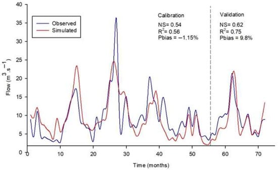
Figure 4.
Hydrograph of observed and simulated monthly streamflows during the calibration and validation periods of the SWAT model at the Itaicá station.
During the calibration period, the simulated flows generally overestimated streamflow values in the first and second years, except for an underestimation at the end of the second year (month 21). In the third and fourth years, streamflows were mostly underestimated, with the exception of months 29 and 39, where overestimations occurred.
During the validation period, streamflows were underestimated, except at the end of the final year—specifically in months 63, 69, and 72—where overestimations were observed.
To assess the SWAT model’s performance, the following three statistical indicators were used: the coefficient of determination (R2), the Nash–Sutcliffe efficiency (NS), and Percent Bias (PBIAS). These indicators are widely adopted in hydrological modeling to evaluate model accuracy and detect tendencies toward under- or overestimation. Numerous studies have used R2, NS, and PBIAS to assess the performance of SWAT when compared to observed data, helping to verify model calibration quality and predictive capability [32,47,51,52,53,54,55,56,57].
Moriasi et al. provided classification thresholds for NS and PBIAS values that help to define model performance quality on a monthly scale [34]. According to these criteria, the SWAT model applied to the Jundiaí River Basin can be rated between satisfactory and good.
For calibration, the R2 (0.56) and NS (0.54) values indicated a satisfactory performance. The PBIAS value of −1.15% was classified as very good, reflecting a slight tendency toward overestimation, yet remaining within acceptable bounds. During validation, there were notable improvements in the coefficient of determination (R2 = 0.75) and NS (0.62), corresponding to a model performance between very good and satisfactory, respectively. The PBIAS value of 9.8% also fell within the “very good” classification, demonstrating the model’s strong capability to replicate observed streamflow.
Similar results were reported by Pontes et al. in simulations using SWAT in the Camanducaia River Basin (southeast Brazil), where PBIAS errors ranged from −10.9% to −1.1% during calibration and validation [58]. When applied to the Jaguari River Basin, PBIAS values of 4.10% during calibration and −3.5% during validation were also recorded, reinforcing the model’s ability to represent the hydrological behavior in these basins.
In a study aimed at supporting water resource management and ecosystem services in the Piracicaba River Basin, ref. [32] found NS coefficients ranging from 0.72 to 0.89 during calibration and from 0.50 to 0.75 during validation for monthly streamflow simulation—again classifying the model performance as satisfactory to very good.
These favorable results may be attributed to the high quality of observed streamflow data, the accurate spatial representation of the basin, and the effectiveness of the calibration process. According to Althoff et al., a PBIAS value within the “very good” range indicates a lack of systematic bias, while the NS value—though satisfactory—may be influenced by limitations in estimating peak flows or by the basin’s complex hydrological features, such as land use and rainfall variability [59].
Another study found that limitations and uncertainties in the SWAT model arise from (i) conceptual simplifications (e.g., the SCS curve number method for flow partitioning), (ii) basin processes not included in the model (e.g., wind erosion and wetland processes), and (iii) processes included in the model but unknown or poorly documented in the study area (e.g., reservoirs, water transfers, and farm-level management practices that affect water quality) [16].
Although the Jundiaí River Basin is one of the smallest in the state of São Paulo, it is among the most industrialized. According to Garcia et al., the basin has a growing vulnerability to extreme precipitation events, such as floods and droughts, due to the combined effects of climate change, intense urbanization, deforestation, and inadequate land use [60]. The authors emphasized that addressing such challenges requires integrated adaptation and mitigation strategies, including infrastructure for flow control, hydrosedimentological monitoring, land use planning, and the conservation of remaining native vegetation—essential for regulating hydrological and climatic functions [60].
Additionally, the results of this study highlight the value of SWAT modeling as a decision support tool for the rational and sustainable management of water resources in the Jundiaí River Basin. Although its application for the assessment of payment for ecosystem services is still limited, the model shows strong potential for quantifying these services and providing technical support for environmental and water management policies.
3.3. Evaluation of the Impacts of Land Use and Land Cover Changes
Table 7 presents the land use and land cover areas for each scenario. The Current Scenario, as the name suggests, reflected the present land use in the Jundiaí River Basin. In Scenario 1, a 50 m riparian buffer zone was enforced along the entire basin, in accordance with the Brazilian Forest Code (Law 12.651/2012). In Scenario 2, 15% of the area originally occupied by pasture/agriculture was converted into forested land.
Table 7.
Land use and land cover areas (%) under current and simulated scenarios.
When comparing the Current Scenario with Scenario 1, it is evident that approximately 2.201% of forest formation areas are currently lost. Furthermore, 0.025% of eucalyptus areas, 0.278% of pasture, 0.01% of sugarcane fields, 0.922% of cropland, 0.773% of urban areas, 0.003% of soybean fields, and 0.09% of other temporary crops are located in riparian zones, which should legally be protected.
In Scenario 2, forest cover accounts for 40.281% of the basin’s total area, an increase of 13.119% compared to the Current Scenario, resulting from the conversion of 15% of pasture/agricultural land to forest.
Hydrological balance variables simulated with SWAT for each scenario are presented in the bar charts in Figure 5A,B. Surface runoff (Qsup) decreases in Scenario 1 (348.16 mm) and Scenario 2 (340.13 mm) compared to the Current Scenario (367.64 mm). This reduction results from greater forest coverage, which promotes increased infiltration.
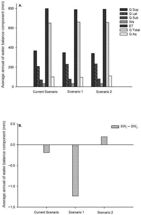
Figure 5.
(A) Annual average of water balance components: surface runoff (QSup), lateral flow (QLat), subsurface flow (QSub), total water in the unsaturated soil zone (Ws), water yield (QTotal), evapotranspiration (ET), and total aquifer recharge (QAq) for the Current, Scenario 1, and Scenario 2. (B) Variation in soil water content (SWt-SWo) for the Current, Scenario 1, and Scenario 2.
According to Tucci [61], greater vegetation cover enhances rainfall interception and root water uptake, increases infiltration and aquifer recharge, and reduces surface runoff, contributing to more stable streamflow.
Lateral flow (Qlat) also increased in Scenario 1 (229.81 mm) and Scenario 2 (232.40 mm) compared to the Current Scenario (207 mm). In SWAT, lateral flow occurs when infiltrated water encounters a less permeable soil layer and is redirected laterally—especially significant in structured or sloped soils [15]. Forested areas tend to preserve soil structure, favoring lateral flow compared to compacted or deforested areas.
Wang et al. found similar results in the Wei River Basin, where converting agricultural land to mixed forest increased lateral flow and decreased surface runoff. This was attributed to the improved soil structure and higher infiltration under forest cover [62].
Subsurface flow (Qsub) also increased in the two reforested scenarios. This component represents the baseflow emerging from shallow aquifers, sustaining rivers even without recent rainfall. Another study noted that this flow increased when reforestation occurred at higher elevations, promoting aquifer recharge and baseflow during dry periods [63].
Dotto [64], simulating riparian forest preservation in the Jaguari River Basin, also observed increased groundwater storage and baseflow. The author emphasized the importance of riparian vegetation in maintaining baseflow and supporting water sustainability [64].
The estimated water content in the unsaturated zone (Ws) remained relatively constant across scenarios (31.22–31.24 mm), consistent with Dotto [64], who reported 32 mm for a similar scenario [64]. Evapotranspiration was slightly lower in Scenario 1 (789 mm) and Scenario 2 (791 mm) compared to the Current Scenario (798.5 mm). Though increased vegetation typically raises evapotranspiration, in this study, reduced surface runoff and increased infiltration explain the lower ET. Similar trends have been reported [64,65], and ref. [66] noted that only intensive reforestation tends to increase evapotranspiration.
Total water yield (Qtotal) increased in Scenario 1 (660.42 mm) and Scenario 2 (657.69 mm) compared to the Current Scenario (650.08 mm) due to improved soil properties and the distinct water demands of each land cover type. Soils with higher infiltration and organic matter content improve water retention and reduce runoff.
Dos Santos et al. emphasized that vegetated areas promote infiltration and water production over time [67]. The variation in soil water content (SWt-SWo) showed a water deficit in the Current Scenario (−0.19 mm) and Scenario 1 (−1.23 mm), but a slight surplus in Scenario 2 (0.19 mm). In SWAT, this variable represents the water retained in the root zone, available for evapotranspiration or percolation.
Although Scenario 1 offered environmental benefits by restoring 2.20% of forested APP area, it reduced agricultural land (e.g., eucalyptus, sugarcane, pasture, and citrus), leading to increased infiltration and lateral flow, which impacted soil water storage. Zhang et al. noted that land use changes—such as reforesting agricultural areas—can enhance rainfall interception and infiltration, although sometimes they reduce soil water storage due to increased percolation [68].
Scenario 2 provided the most favorable hydrological balance for the Jundiaí River Basin, mainly due to the more extensive conversion of pasture/agriculture to forest. This transformation improved infiltration, aquifer recharge, and reduced runoff—indicating increased year-round water availability. Studies by [65,69] and ref. [70] support this finding, highlighting the importance of forest cover in water balance improvement in water-stressed basins.
Annual sediment yield decreased in Scenario 1 (6.018 t/ha) and Scenario 2 (5.772 t/ha) compared to the Current Scenario (6.177 t/ha), as shown in Figure 6. This reduction was attributed to riparian vegetation acting as a barrier and increased forest areas that produced lower sediment loads. Similarly, Paz et al. found lower sediment production in reforested scenarios due to protective vegetation cover and reduced soil exposure to erosion [36].
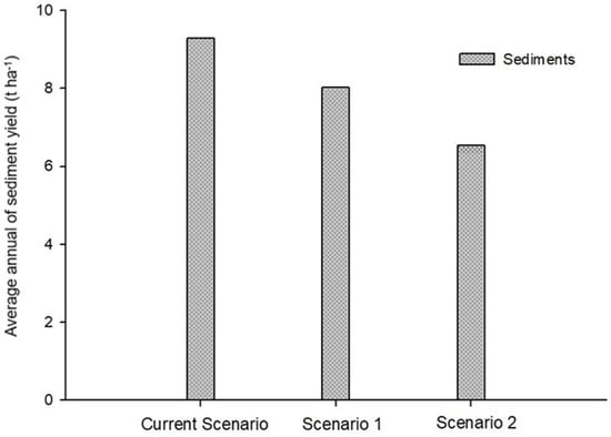
Figure 6.
Annual average sediment yield (t·ha-1) for the Current, Scenario 1, and Scenario 2.
In SWAT, sediment production is based on laminar erosion processes via a modified USLE equation, which incorporates runoff volume, vegetation cover, and soil erodibility [15].
Riparian and forest vegetation play a critical role in soil protection by buffering rainfall impact, reducing runoff, and minimizing erosion and sediment generation. Studies by [71,72] underscore the importance of preserving native vegetation to control sedimentation.
Martins et al., in simulations of riparian APP recovery in the Jundiaí-Mirim River Basin, observed up to a 30% reduction in sediment production [73]. They attributed this to native vegetation’s root systems and litter layers acting as natural erosion barriers.
Figure 7, Figure 8, Figure 9 and Figure 10 below show the spatial distribution of surface runoff (SURQ), evapotranspiration (ET), soil water storage (AWC), lateral and baseflow (GWQ), and sediment yield (SED).
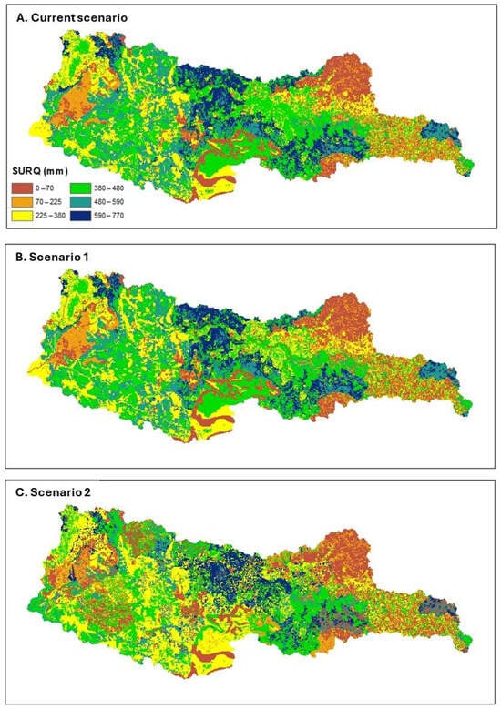
Figure 7.
Spatial distribution of surface runoff (SURQ) under the different simulated scenarios: (A) represents the current scenario; (B) represents Scenario 1; (C) represents Scenario 2.
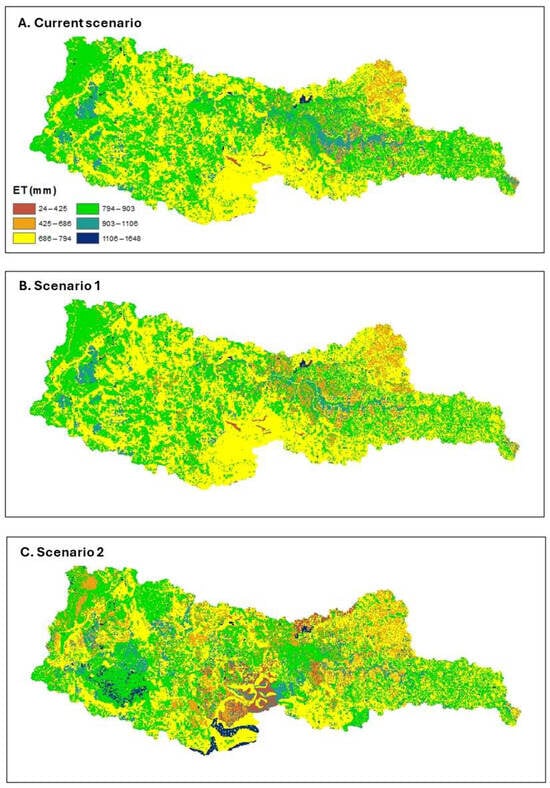
Figure 8.
Spatial distribution of evapotranspiration (ET) under the different simulated scenarios: (A) represents the current scenario; (B) represents Scenario 1; (C) represents Scenario 2.
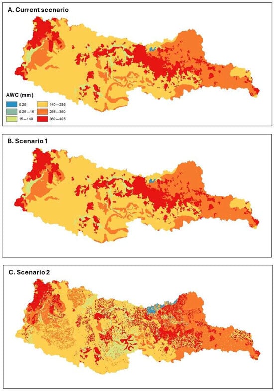
Figure 9.
Spatial distribution of soil water storage (AWC) under the different simulated scenarios: (A) represents the current scenario; (B) represents Scenario 1; (C) represents Scenario 2.
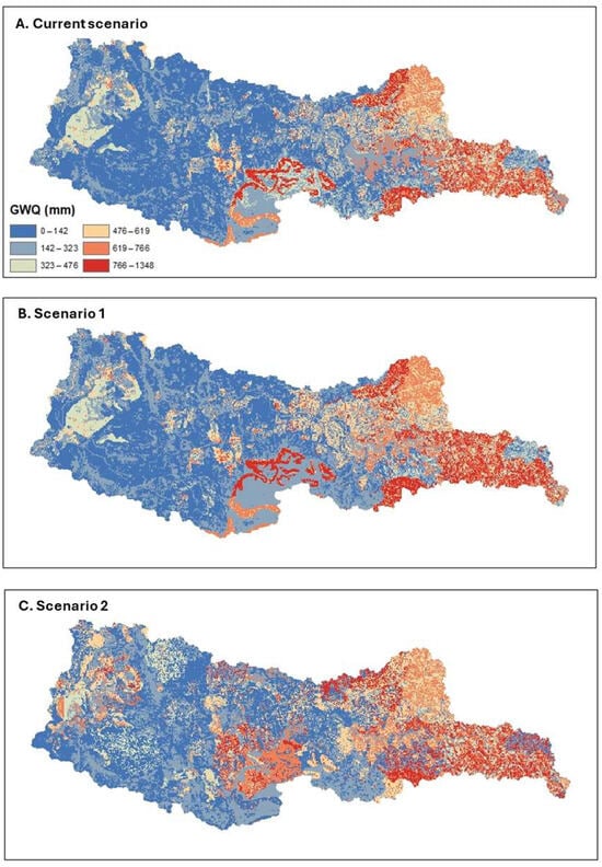
Figure 10.
Spatial distribution of baseflow (GWQ) under the different simulated scenarios: (A) represents the current scenario; (B) represents Scenario 1; (C) represents Scenario 2.
SWAT generated outputs for the main components of the water balance at the HRU level, along with vector files (shapefiles) corresponding to the spatial boundaries of these HRUs. The numerical results were exported to spreadsheets and integrated with the shapefiles in the ArcGIS environment. The association between tabular data and spatial geometries was determined using the Join Attributes tool, enabling the generation of thematic maps for variables such as surface runoff, evapotranspiration, and sediment yield. This procedure allowed for a spatial analysis of the hydrological processes simulated by the model.
In Figure 7B, a reduction in urban surface runoff is visible due to preserved riparian zones in Scenario 1. Figure 7C shows reduced runoff in areas converted from pasture/agriculture to forest.
Although total evapotranspiration decreased across the basin, spatial analysis (Figure 8C) revealed localized increases in areas with new forest cover compared to Figure 8A.
Figure 9A,B show minimal spatial changes in soil water storage in Scenario 1, while Figure 8C reveals increases in reforested areas.
Figure 10 shows an evident increase in baseflow in Scenarios 1 and 2 (Figure 10B,C) compared to the Current Scenario (Figure 10A), confirming that riparian and forest expansion enhance infiltration and aquifer recharge, supporting sustained streamflow.
Sediment yield maps (Figure 11B,C) show significant reductions in reforested and protected riparian areas compared to Figure 11A.
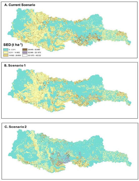
Figure 11.
Spatial distribution of sediment yield (SED) under the different simulated scenarios: (A) represents the current scenario; (B) represents Scenario 1; (C) represents Scenario 2.
Water and sediment production in a watershed are strongly linked to anthropogenic changes in land use and cover. These changes directly affect hydrosedimentological processes, underscoring the need for sustainable land management to ensure both water quantity and quality.
According to Balist et al., water availability is closely tied to land use and cover, as each type influences infiltration, runoff, and vegetation density—key elements of the water balance [74]. Thus, effective land use monitoring and planning are essential for accurate water resource estimation and long-term sustainability.
The scenario simulations performed in the Jundiaí River Basin clearly showed that land use and cover influence the basin’s hydrological regime by altering rainfall interception, surface runoff, and infiltration—core components of the hydrological cycle. In this context, the SWAT (Soil and Water Assessment Tool) model proved to be a valuable tool for public managers, enabling simulations of alternative land use scenarios.
The application of the SWAT model in the present study finds parallels in both national and international contexts, which highlights its singularity, as well as its universality. In Brazil, a study employed SWAT with semi-automated calibration (SWAT-CUP + SUFI-2) to simulate streamflow in the Ibicuí River Basin from 2011 to 2020, using climate data, land use maps, soil, and topographic data. The model showed an excellent statistical performance, with a Nash–Sutcliffe Efficiency (NSE) of 0.87 for calibration and 0.88 for validation and a Percent Bias (PBIAS) of −14.1% and −22.2%, respectively [75]. These results indicate a high potential for SWAT to reliably estimate streamflow, even in data-scarce regions, reinforcing its usefulness as a decision support tool for regional water resource management.
Complementarily, in an international context, another study, [76], applied SWAT to model the monthly water balance in the Wadi Mina Basin, a semi-arid region in northwestern Algeria. The study used spatial data (DEM, soil, and land use) and meteorological data (precipitation, temperature, humidity, radiation, and wind), calibrating the model for the period from January 2012 to August 2013 and validating it until December 2014. The performance was considered good, with NSE values of 0.79 (calibration) and 0.69 (validation) and PBIAS values of 8.5% and 11.4%, respectively. Additionally, the study quantified the main components of the water balance: approximately 71% of rainfall was lost through evapotranspiration, while the remaining 29% contributed to surface runoff or infiltration.
Furthermore, the results obtained through SWAT provide critical support for water resource management decision making in a basin that still lacks technical data and tools. While SWAT’s use in payment for ecosystem services (PES) assessments is still limited, it demonstrates strong potential for quantifying ecosystem services and guiding evidence-based policies for environmental and water resource conservation.
4. Conclusions and Recommendations
The SWAT model requires a large number of input parameters for its execution, making sensitivity analysis an essential tool for reducing model complexity and identifying the most influential parameters for effective calibration. In this study, the model showed a better performance during the validation period.
Parameters related to surface runoff were the most sensitive in simulating streamflow in the Jundiaí River Basin. Based on the statistical indicators R2, Nash–Sutcliffe efficiency (NS), and Percent Bias (PBIAS), the SWAT model was able to adequately simulate monthly streamflows, even under conditions of limited spatial data, demonstrating good agreement between observed and simulated values.
A comprehensive understanding of the processes that directly or indirectly influence the hydrological behavior of the Jundiaí River Basin is a key element in supporting informed decision making for sustainable water resource management and conservation. The use of the SWAT model enables not only the evaluation of historical and current land use scenarios, but also the projection of future scenarios quickly and at a low cost.
Among the scenarios analyzed, Scenario 2, in which 15% of the area originally used for pasture and agriculture was converted into forest, yielded the most favorable hydrological outcomes. Increased water infiltration and aquifer recharge, along with reduced surface runoff and sediment yield, indicate that forest restoration practices can significantly enhance water availability and quality in the basin.
The calibration and validation of the SWAT model for the Jundiaí River Basin not only confirmed its ability to adequately represent local hydrological processes, but also established a solid methodological foundation for future applications. Once calibrated, the model becomes a versatile tool for developing studies focused on simulating climate change, evaluating conservation management practices, analyzing land use and occupation policies, and planning strategies for water conservation and security.
The results of this study reinforce the importance of hydrological assessments based on land use and land cover scenarios as a decision support tool for the Jundiaí River Basin. It is noteworthy that the analysis of reforestation scenarios aimed at improving water balance becomes even more effective when integrated with water resource management, ecosystem service valuation, and analysis of economic indicators. This integrated approach enables a more comprehensive and accurate understanding of long-term environmental and socioeconomic benefits, supporting the development of more efficient and well-founded ecological restoration strategies. The use of tools such as the SWAT model, combined with implementation cost estimates and ecosystem service valuation, represents a valuable resource to support public and private decision making, promoting more sustainable land use planning in the Jundiaí River Basin.
Given the results obtained, it is recommended that public managers and environmental planning agencies consider incorporating hydrological models such as SWAT into the policy formulation process for land use and occupation. The implementation of forest restoration programs, especially in critical areas such as riverbanks and regions with a high susceptibility to erosion, should be prioritized, given their positive impact on regulating water flow and reducing soil loss. In addition, the integration of model results with economic indicators can contribute to the development of payment for environmental services (PES) mechanisms, strengthening sustainable water management and land use initiatives in the Jundiaí River Basin.
Author Contributions
Conceptualization, L.B.M., T.R.L. and M.V.F.; methodology, L.B.M. and T.R.L.; software, L.B.M.; validation, L.B.M. and T.R.L.; formal analysis, L.B.M.; writing—original draft preparation, L.B.M.; writing—review and editing, T.R.L., P.S. and S.N.D.; visualization, T.R.L. and P.S.; supervision, M.V.F., S.N.D. and T.R.L.; funding acquisition, M.V.F. and S.N.D. All authors have read and agreed to the published version of the manuscript.
Funding
This research was funded by CAPES (Coordination for the Improvement of Higher Education Personnel, Brazil), grant number 88887.513601/2020.
Data Availability Statement
Authors will make data available under request.
Conflicts of Interest
The authors declare no conflicts of interest.
Abbreviations
| Abbreviation | Definition |
| SWAT | Soil and Water Assessment Tool |
| HRU | Hydrological Response Unit |
| DEM | Digital Elevation Model |
| ET | Evapotranspiration |
| SURQ | Surface Runoff |
| QSup | Surface Runoff (Hydrological Output) |
| QLat | Lateral Flow |
| QSub | Subsurface Flow (Baseflow) |
| QAq | Total Aquifer Recharge |
| QTotal | Total Water Yield |
| Ws | Water Storage in the Unsaturated Zone |
| SWt–SWo | Change in Soil Water Content |
| AWC | Available Water Content |
| GWQ | Groundwater Flow (Baseflow in SWAT) |
| SED | Sediment Yield |
| R2 | Coefficient of Determination |
| NS | Nash–Sutcliffe Efficiency |
| PBIAS | Percent Bias |
| APP | Permanent Preservation Area (Área de Preservação Permanente) |
| AMC II | Antecedent Moisture Condition II |
| CN2 | Curve Number for AMC II Condition |
| OV_N | Manning’s n Coefficient for Overland Flow |
| GWQMN | Threshold Depth of Water in Shallow Aquifer for Return Flow |
| ALPHA_BF | Baseflow Recession Constant |
| SOL_BD | Bulk Density of the Soil |
| SOL_AWC | Available Water Capacity |
| SURLAG | Surface Runoff Lag Time |
| LAT_TTIME | Lateral Flow Travel Time |
| REVAPMN | Threshold Depth for Revap from Shallow Aquifer |
| GW_REVAP | Groundwater Revap Coefficient |
References
- Marengo, J.A.; Alves, L.M. Crise Hídrica Em São Paulo Em 2014: Seca e Desmatamento; GEOUSP Espaço e Tempo (Online): São Paulo, Brazil, 2015; Volume 19, pp. 485–494. [Google Scholar]
- Custódio, V. A Crise Hídrica Na Região Metropolitana de São Paulo (2014–2015). Espaço Tempo 2015, 19, 445–463. [Google Scholar]
- Richter, R.M.; Jacobi, P.R. Conflitos Na Macrometrópole Paulista Pela Perspectiva Da Crise Hídrica|Conflicts in the São Paulo Macrometropolis from the Perspective of the Water Crisis. Rev. Bras. Estud. Urbanos Reg. 2018, 20, 556. [Google Scholar] [CrossRef]
- Tucci, C.E.M. Águas Urbanas. Estud. Avançados 2008, 22, 97–112. [Google Scholar] [CrossRef]
- Neto, J.C.C. A Crise Hídrica No Estado de São Paulo; GEOUSP Espaço E Tempo (Online): São Paulo, Brazil, 2015; Volume 19, pp. 479–484. [Google Scholar]
- Soriano, É.; Londe, L.d.R.; Di Gregorio, L.T.; Coutinho, M.P.; Santos, L.B.L. Water Crisis in São Paulo Evaluated under the Disaster’s Point of View. Ambiente Soc. 2016, 19, 21–42. [Google Scholar] [CrossRef]
- Neves, M.A.; Pereira, S.Y.; Fowler, H.G. Impactos Do Sistema Estadual de Gerenciamento de Recursos Hídricos Na Bacia Do Rio Jundiaí (SP). Ambiente Soc. 2007, 10, 149–160. [Google Scholar] [CrossRef]
- Riediger, P.I.; Marques, G.F.; Dalcin, A.P.; Jardin, P.F.; Magalhães Filho, F.J.C.; Persson, K.M. Improving Sanitation Strategies through Coordinated Investment on Wastewater Treatment Reuse and Water Supply at the Watershed Scale: A Brazilian View of Water Security. Water Policy 2025, 27, 182–203. [Google Scholar] [CrossRef]
- Guan, M.; Sillanpää, N.; Koivusalo, H. Modelling and Assessment of Hydrological Changes in a Developing Urban Catchment. Hydrol. Process 2015, 29, 2880–2894. [Google Scholar] [CrossRef]
- Moura, L.B.; Lopes, T.R.; Folegatti, M.V.; Duarte, S.N.; Oliveira, R.K. Hydrological Simulation in the Corumbataí River Basin Using the SWAT Model: Simulation of Hydrological Variables and Land Use and Land Cover Scenarios. J. Hydrol. Eng. 2025, 30, 05024024. [Google Scholar] [CrossRef]
- Hung, C.-L.J.; James, L.A.; Carbone, G.J.; Williams, J.M. Impacts of Combined Land-Use and Climate Change on Streamflow in Two Nested Catchments in the Southeastern United States. Ecol. Eng. 2020, 143, 105665. [Google Scholar] [CrossRef]
- Lopes, T.R.; Folegatti, M.V.; Duarte, S.N.; Moster, C.; Zolin, C.A.; Oliveira, R.K.; Moura, L.B. Economic Value of Environmental Services Regulating Flow and Maintaining Water Quality in the Piracicaba River Basin, Brazil. J. Water Resour. Plan Manag. 2023, 149, 05023008. [Google Scholar] [CrossRef]
- Zhang, L.; Nan, Z.; Yu, W.; Ge, Y. Hydrological Responses to Land-Use Change Scenarios under Constant and Changed Climatic Conditions. Environ. Manag. 2016, 57, 412–431. [Google Scholar] [CrossRef]
- Honda, E.A.; Durigan, G. A Restauração de Ecossistemas e a Produção de Água. Hoehnea 2017, 44, 315–327. [Google Scholar] [CrossRef]
- Neitsch, S.L.; Arnold, J.G.; Kiniry, J.R.; Williams, J.R. Soil and Water Assessment Tool Theoretical Documentation Version 2009, 1st ed.; Texas A&M: College Station, TX, USA, 2011; Volume 1. [Google Scholar]
- Abbaspour, K.C.; Rouholahnejad, E.; Vaghefi, S.; Srinivasan, R.; Yang, H.; Kløve, B. A Continental-Scale Hydrology and Water Quality Model for Europe: Calibration and Uncertainty of a High-Resolution Large-Scale SWAT Model. J. Hydrol. 2015, 524, 733–752. [Google Scholar] [CrossRef]
- Wang, W.; Du, Y.; Chau, K.; Cheng, C.-T.; Xu, D.; Zhuang, W.-T. Evaluating the Performance of Several Data Preprocessing Methods Based on GRU in Forecasting Monthly Runoff Time Series. Water Resour. Manag. 2024, 38, 3135–3152. [Google Scholar] [CrossRef]
- Wenchuan, W.; Yanwei, Z.; Dongmei, X.; Yanghao, H. Error Correction Method Based on Deep Learning for Improving the Accuracy of Conceptual Rainfall-Runoff Model. J. Hydrol. 2024, 643, 131992. [Google Scholar] [CrossRef]
- Comitê da Bacia dos Rios Piracicaba, J.e.C. Plano Das Bacias Hidrográficas Dos Rios Piracicaba, Capivari e Jundiaí 2010–2020. Available online: https://www.comitespcj.org.br/ (accessed on 23 May 2025).
- MapaBiomas Maps and Data. Available online: http://mapbiomas.org/ (accessed on 23 May 2025).
- Puga, B.P.; Garcia, J.R.; Maia, A.G. Governança Dos Recursos Hídricos Na Bacia Do Rio Jundiaí (São Paulo). Revibec Rev. Iberoam. Econ. Ecológica 2020, 32, 93–101. [Google Scholar]
- ANA Water Production Program. Available online: http://www3.ana.gov.br/portal/ANA/programas-e-projetos/copy_of_produtor-de-agua (accessed on 23 May 2025).
- Brazilian National Institute of Meteorology Average Climate Data of Brazil from 1961. Available online: http://www.inmet.gov.br/portal/index.php?r=clima/normaisclimatologicas (accessed on 23 May 2025).
- Sharpley, A.N.; Williams, J.R. Erosion/Productivity Impact Calculator. Model Documentation, 1st ed.; USDA: Washington, DC, USA, 1990; Volume 1. [Google Scholar]
- Arnold, J.G.; Srinivasan, R.; Muttiah, R.S.; Williams, J.R. Large Area Hydrologic Modeling and Assessment Part I: Model Development 1. JAWRA J. Am. Water Resour. Assoc. 1998, 34, 73–89. [Google Scholar] [CrossRef]
- ANA Brazilian National Water Agency Annual Report. Available online: https://www.gov.br/ana/pt-br (accessed on 29 June 2025).
- Rossi, M. Mapa Pedológico Do Estado de São Paulo: Revisado e Ampliado, 1st ed.; Instituto Florestal: São Paulo, SP, Brazil, 2017; Volume 1. [Google Scholar]
- Santos, H.; Junior, W.C.; Dart, R.O.; Áglio, M.L.D.; Souza, J.; Pares, J.G.; Oliveira, A.P. O Novo Mapa de Solos do Brasil: Legenda Atualizada, 1st ed.; EMBRAPA Solos: Rio de Janeiro, RJ, Brazil, 2011; Volume 1. [Google Scholar]
- Mingoti, R.; Spadotto, C.A.; Moraes, D.A.d.C. Suscetibilidade à Contaminação Da Água Subterrânea Em Função de Propriedades Dos Solos No Cerrado Brasileiro. Pesqui Agropecu Bras 2016, 51, 1252–1260. [Google Scholar] [CrossRef]
- Farr, T.G.; Rosen, P.A.; Caro, E.; Crippen, R.; Duren, R.; Hensley, S.; Kobrick, M.; Paller, M.; Rodriguez, E.; Roth, L.; et al. The Shuttle Radar Topography Mission. Rev. Geophys. 2007, 45. [Google Scholar] [CrossRef]
- van Griensven, A.; Meixner, T.; Grunwald, S.; Bishop, T.; Diluzio, M.; Srinivasan, R. A Global Sensitivity Analysis Tool for the Parameters of Multi-Variable Catchment Models. J. Hydrol. 2006, 324, 10–23. [Google Scholar] [CrossRef]
- Lopes, T.R.; Folegatti, M.V.; Duarte, S.N.; Zolin, C.A.; Fraga Junior, L.S.; Moura, L.B.; Oliveira, R.K.; Santos, O.N.A. Hydrological Modeling for the Piracicaba River Basin to Support Water Management and Ecosystem Services. J. S. Am. Earth Sci. 2020, 103, 102752. [Google Scholar] [CrossRef]
- Aragão, R.d.; Cruz, M.A.S.; Amorim, J.R.A.d.; Mendonça, L.C.; Figueiredo, E.E.d.; Srinivasan, V.S. Análise de Sensibilidade Dos Parâmetros Do Modelo SWAT e Simulação Dos Processos Hidrossedimentológicos Em Uma Bacia No Agreste Nordestino. Rev. Bras. Ciência Solo 2013, 37, 1091–1102. [Google Scholar] [CrossRef]
- Moriasi, D.N.; Arnold, J.G.; Van Liew, M.W.; Bingner, R.L.; Harmel, R.D.; Veith, T.L. Model Evaluation Guidelines for Systematic Quantification of Accuracy in Watershed Simulations. Trans. ASABE 2007, 50, 885–900. [Google Scholar] [CrossRef]
- Devia, G.K.; Ganasri, B.P.; Dwarakish, G.S. A Review on Hydrological Models. Aquat. Procedia 2015, 4, 1001–1007. [Google Scholar] [CrossRef]
- Paz, Y.M.; Freire-Silva, J.; Holanda, R.M.d.; Galvincio, J.D. Planejamento e Gestão Ambiental de Bacias Hidrográficas a Partir Da Modelagem Hidrossedimentológica e Estudo de Cenários Alternativos de Uso e Cobertura Do Solo. Geosciences 2023, 41, 675–687. [Google Scholar] [CrossRef]
- Singh, A.; Jha, S.K. Identification of Sensitive Parameters in Daily and Monthly Hydrological Simulations in Small to Large Catchments in Central India. J. Hydrol. 2021, 601, 126632. [Google Scholar] [CrossRef]
- Mendonça dos Santos, F.; Proença de Oliveira, R.; Augusto Di Lollo, J. Effects of Land Use Changes on Streamflow and Sediment Yield in Atibaia River Basin—SP, Brazil. Water 2020, 12, 1711. [Google Scholar] [CrossRef]
- Bressiani, D.A. Coping with Hydrological Risks Through Flooding Riskindex, Complex Watershed Modeling, Different Calibration Techniques, and Ensemble Streamflow Forecasting; University of São Paulo: Piracicaba, SP, Brazil, 2016. [Google Scholar]
- Pereira, D.d.R.; Martinez, M.A.; Pruski, F.F.; da Silva, D.D. Hydrological Simulation in a Basin of Typical Tropical Climate and Soil Using the SWAT Model Part I: Calibration and Validation Tests. J. Hydrol. Reg. Stud. 2016, 7, 14–37. [Google Scholar] [CrossRef]
- Hussain, S.; Niyazi, B.; Elfeki, A.M.; Masoud, M.; Wang, X.; Awais, M. SWAT-Driven Exploration of Runoff Dynamics in Hyper-Arid Region, Saudi Arabia: Implications for Hydrological Understanding. Water 2024, 16, 2043. [Google Scholar] [CrossRef]
- Andrade, C.W.L.d.; Montenegro, S.M.G.L.; Lima, J.R.d.S.; Montenegro, A.A.d.A.; Srinivasan, R. Sensitivity Analysis of SWAT Model Parameters Applied in a Sub-Basin of Northeast Region, Brazil. Rev. Bras. Geogr. Física 2017, 10, 440–453. [Google Scholar] [CrossRef][Green Version]
- Li, M.; Di, Z.; Duan, Q. Effect of Sensitivity Analysis on Parameter Optimization: Case Study Based on Streamflow Simulations Using the SWAT Model in China. J. Hydrol. 2021, 603, 126896. [Google Scholar] [CrossRef]
- Jovino, E.S. Impactos do Uso da Terra na Produção de Sedimentos Em Bacia Hidrográfica Tropical; Federal University of Rio Grande Do Norte: Natal, RN, Brazil, 2021. [Google Scholar]
- Hosseini, S.H.; Memarian, H.; Memarian, H.; Khaleghi, M.R. Application of SWAT Model and SWAT-CUP Software in Simulation and Analysis of Sediment Uncertainty in Arid and Semi-Arid Watersheds (Case Study: The Zoshk–Abardeh Watershed). Model Earth Syst. Environ. 2020, 6, 2003–2013. [Google Scholar] [CrossRef]
- Brighenti, T.; Bonumá, N.; Chaffe, P. Calibração Hierárquica Do Modelo Swat Em Uma Bacia Hidrográfica Catarinense. Rev. Bras. Recur. Hídricos 2016, 21, 53–64. [Google Scholar] [CrossRef]
- Fukunaga, D.C.; Cecílio, R.A.; Zanetti, S.S.; Oliveira, L.T.; Caiado, M.A.C. Application of the SWAT Hydrologic Model to a Tropical Watershed at Brazil. Catena 2015, 125, 206–213. [Google Scholar] [CrossRef]
- Kuwajima, J.I. Análise do Modelo SWAT Como Ferramenta de Prevenção e de Estimativa de Assoreamento no Reservatório do Lobo (Itirapina/Brotas/SP); Federal University of São Carlos: São Carlos, Brazil, 2012. [Google Scholar]
- Arnold, J.G.; Moriasi, D.N.; Gassman, P.W.; Abbaspour, K.C.; White, M.J.; Srinivasan, R.; Santhi, C.; Harmel, R.D.; van Griensven, A.; Van Liew, M.W.; et al. SWAT: Model Use, Calibration, and Validation. Trans. ASABE 2012, 55, 1491–1508. [Google Scholar] [CrossRef]
- Blainski, É.; Acosta, E.; Prado Nogueira, P.C. Calibração e Validação Do Modelo SWAT Para Simulação Hidrológica Em Uma Bacia Hidrográfica Do Litoral Norte Catarinense. Ambiente Agua-Interdiscip. J. Appl. Sci. 2017, 12, 226. [Google Scholar] [CrossRef]
- Almeida, A.L.S.P.; Macedo, D.R.; Santos, H.d.A.e.; Ribeiro, S.M.C.; Hughes, R.M. Managing Water Resources in Complex Tropical Basins: Tailored SWAT Ecohydrological Modeling to the Rio Das Velhas, Brazil. RBRH 2023, 28, e33. [Google Scholar] [CrossRef]
- Galbetti, M.V. Avaliação dos Efeitos Hidrológicos da Aplicação de Cenários Propostos Pelo Poder Público; State University of Campinas: Campinas, Brazil, 2021. [Google Scholar]
- Haas, M.B.; Guse, B.; Fohrer, N. Assessing the Impacts of Best Management Practices on Nitrate Pollution in an Agricultural Dominated Lowland Catchment Considering Environmental Protection versus Economic Development. J. Environ. Manag. 2017, 196, 347–364. [Google Scholar] [CrossRef]
- Franco, A.C.L. Calibração do Modelo SWAT Com Evapotranspiração Proveniente de Sensoriamento Remoto e Vazão Observada; Federal University of Santa Catarina: Florianópolis, Brazil, 2017. [Google Scholar]
- Me, W.; Abell, J.M.; Hamilton, D.P. Effects of Hydrologic Conditions on SWAT Model Performance and Parameter Sensitivity for a Small, Mixed Land Use Catchment in New Zealand. Hydrol. Earth Syst. Sci. 2015, 19, 4127–4147. [Google Scholar] [CrossRef]
- Neto, J.; Silva, A.; Mello, C.; Júnior, A. Simulação Hidrológica Escalar Com o Modelo SWAT. Rev. Bras. Recur. Hídricos 2014, 19, 177–188. [Google Scholar] [CrossRef]
- Lubitz, E.; Pinheiro, A.; Kaufmann, V. Simulação Do Transporte de Sedimentos, Nitrogênio e Fósforo Na Bacia Do Ribeirão Concórdia, SC. Rev. Bras. Recur. Hídricos 2013, 18, 39–54. [Google Scholar] [CrossRef]
- Pontes, L.M.; Viola, M.R.; Silva, M.L.N.; Bispo, D.F.A.; Curi, N. Hydrological Modeling of Tributaries of Cantareira System, Southeast Brazil, with the Swat Model. Eng. Agrícola 2016, 36, 1037–1049. [Google Scholar] [CrossRef]
- Althoff, D.; Rodrigues, L.N. Goodness-of-Fit Criteria for Hydrological Models: Model Calibration and Performance Assessment. J. Hydrol. 2021, 600, 126674. [Google Scholar] [CrossRef]
- Garcia, J.R.; Miyamoto, B.C.B.; Maia, A.G. Eventos Extremos de Precipitação: Identificação e Análise Da Bacia Hidrográfica Do Rio Jundiaí, São Paulo. Confins 2018, 37, 1–15. [Google Scholar] [CrossRef]
- Tucci, C.E.M. Hidrologia Ciência e Aplicação, 2nd ed.; Editora da UFRGS: Porto Alegre, Brazil, 2001; Volume 1. [Google Scholar]
- Wang, H.; Sun, F.; Xia, J.; Liu, W. Impact of LUCC on Streamflow Based on the SWAT Model over the Wei River Basin on the Loess Plateau in China. Hydrol. Earth Syst. Sci. 2017, 21, 1929–1945. [Google Scholar] [CrossRef]
- Cecílio, R.A.; Pimentel, S.M.; Zanetti, S.S. Modeling the Influence of Forest Cover on Streamflows by Different Approaches. Catena 2019, 178, 49–58. [Google Scholar] [CrossRef]
- Dotto, A.V.E. Aplicação do Modelo Swat Para Estudo de Cenários Hidrológicos na Bacia Hidrográfica do Rio Jaguari-RS; Federal University of Santa Maria: Santa Maria, RS, Brazil, 2024. [Google Scholar]
- Rodrigues, E.L.; Elmiro, M.A.T.; Jacobi, C.M.; Lamounier, W.L. Aplicação Do Modelo SWAT Na Avaliação Do Consumo de Água Em Áreas de Florestas Plantadas Na Bacia Do Rio Pará, Alto São Francisco, Em Minas Gerais. Soc. Nat. 2015, 27, 485–500. [Google Scholar] [CrossRef]
- Gomes, L.C.; Bianchi, F.J.J.A.; Cardoso, I.M.; Schulte, R.P.O.; Fernandes, R.B.A.; Fernandes-Filho, E.I. Disentangling the Historic and Future Impacts of Land Use Changes and Climate Variability on the Hydrology of a Mountain Region in Brazil. J. Hydrol. 2021, 594, 125650. [Google Scholar] [CrossRef]
- Santos, K.F.d.; Barbosa, F.T.; Bertol, I.; Werner, R.D.S.; Wolschick, N.H.; Mota, J.M. Study of Soil Physical Properties and Water Infiltration Rates in Different Types of Land Use. Semin. Ciências Agrárias 2018, 39, 87. [Google Scholar] [CrossRef]
- Zhang, L.; Wang, C.; Liang, G.; Cui, Y.; Zhang, Q. Influence of Land Use Change on Hydrological Cycle: Application of SWAT to Su-Mi-Huai Area in Beijing, China. Water 2020, 12, 3164. [Google Scholar] [CrossRef]
- Boisramé, G.F.S.; Thompson, S.E.; Tague, C.; Stephens, S.L. Restoring a Natural Fire Regime Alters the Water Balance of a Sierra Nevada Catchment. Water Resour. Res. 2019, 55, 5751–5769. [Google Scholar] [CrossRef]
- Hidayat, Y.; Rachman, L.M.; Wahjunie, E.D.; Baskoro, D.P.T.; Purwakusuma, W.; Yusuf, S.M.; Araswati, F.D. Water Balance Prediction by Simulating Land Use Planning and Water Retention Infrastructure in Upper Cisadane Sub-Watershed, West Java, Indonesia. J. Nat. Resour. Environ. Manag. 2024, 14, 415. [Google Scholar] [CrossRef]
- Mizuno, T.; Kojima, N.; Asano, S. The Risk Reduction Effect of Sediment Production Rate by Understory Coverage Rate in Granite Area Mountain Forest. Sci. Rep. 2021, 11, 14415. [Google Scholar] [CrossRef] [PubMed]
- Pizarro, R.; García-Chevesich, P.; Ingram, B.; Sangüesa, C.; Pino, J.; Ibáñez, A.; Mendoza, R.; Vallejos, C.; Pérez, F.; Flores, J.P.; et al. Establishment of Monterrey Pine (Pinus Radiata) Plantations and Their Effects on Seasonal Sediment Yield in Central Chile. Sustainability 2023, 15, 6052. [Google Scholar] [CrossRef]
- Martins, W.A.; Martins, L.L.; Maria, I.C.D.; Moraes, J.F.L.d.; Pedro Júnior, M.J. Reduction of Sediment Yield by Riparian Vegetation Recovery at Distinct Levels of Soil Erosion in a Tropical Watershed. Ciência Agrotecnologia 2021, 45, e028220. [Google Scholar] [CrossRef]
- Balist, J.; Malekmohammadi, B.; Jafari, H.R.; Nohegar, A.; Geneletti, D. Detecting Land Use and Climate Impacts on Water Yield Ecosystem Service in Arid and Semi-Arid Areas. A Study in Sirvan River Basin-Iran. Appl. Water Sci. 2022, 12, 4. [Google Scholar] [CrossRef]
- Scariot, A.R. Simulação de Vazão Com o Modelo SWAT na Bacia Hidrográfica do Rio Ibicuí/RS; Federal University of Santa Maria: Santa Maria, Brazil, 2023. [Google Scholar]
- Mebarki, H.; Maref, N.; Dris, M.E.-A. Modelling the Monthly Hydrological Balance Using Soil and Water Assessment Tool (SWAT) Model: A Case Study of the Wadi Mina Upstream Watershed. J. Groundw. Sci. Eng. 2024, 12, 161–177. [Google Scholar] [CrossRef]
Disclaimer/Publisher’s Note: The statements, opinions and data contained in all publications are solely those of the individual author(s) and contributor(s) and not of MDPI and/or the editor(s). MDPI and/or the editor(s) disclaim responsibility for any injury to people or property resulting from any ideas, methods, instructions or products referred to in the content. |
© 2025 by the authors. Licensee MDPI, Basel, Switzerland. This article is an open access article distributed under the terms and conditions of the Creative Commons Attribution (CC BY) license (https://creativecommons.org/licenses/by/4.0/).