Article

Assessment and Quantitative Evaluation of Loess Area Geomorphodiversity Using Multiresolution DTMs (Roztocze Region, SE Poland)

Institute of Earth and Environmental Sciences, Maria Curie-Skłodowska University, 20-718 Lublin, Poland
*
Author to whom correspondence should be addressed.
Resources 2023, 12(1), 7; https://doi.org/10.3390/resources12010007
Submission received: 13 October 2022 / Revised: 16 December 2022 / Accepted: 26 December 2022 / Published: 3 January 2023
(This article belongs to the Special Issue Geodiversity Assessment: What, Why and How?)

Abstract

:
The geodiversity of loess areas is reflected in the characteristic dataset of loess landforms, with the dominance of several types of valley forms (mainly gullies). The availability of satellite elevation data and high-resolution aerial topography scanning data provides an opportunity for quantitative assessment of geomorphodiversity. This is done through the analysis of topographic texture, delimitation and statistical characterization of the topographic parameters of erosional landforms, such as volume and degree of dissection (density of valleys) or the degree of ‘coverage’ of the area by valley forms. An important factor affecting the accuracy of the estimation is the accuracy of the underlying digital terrain model (DTM). This study compares three digital terrain models, with cell sizes of 30, 10 and 1 m, generated from satellite altimetry data and airborne laser scanning (ALS) data. The subregion of Szczebrzeszyn Roztocze (Western Roztocze Region, SE Poland), i.e., one of the most typical loess relief regions in Poland, was selected as the study area. Selected topographic texture analyses were carried out using the SLRM (Simple Local Relief Model) algorithm. Delimitation of valleys was performed by delineating the extent of slope change in two key steps: (1) detection of areas below the average topographic surface; (2) delimitation using supervised classification of DTMs. The results of the study show that the accuracy of delimitation of valleys increases inversely proportional to the DTMs resolution. Automated topographic texture analysis allows delimitation and extraction, as well as statistical analysis of parameters of valleys. Finally, two indicators have been proposed, Relative Valley Area (RVA) and Area-normalised Valley Cubature (AVC), which can be used in geomorphodiversity studies of a geologically homogeneous area. The dimensionless RVA index can also be expressed as a percentage (%) of the area of valley forms in a basic field of 1 km2. Furthermore, the AVC index shows the dynamic character of the main relief features of the analysed area.

1. Introduction

Geodiversity is most often understood as a feature of abiotic elements of the environment. Among the various conceptual approaches, the geological concept of geodiversity [1,2] was one of the first to emerge, and it was further developed as part of the lithosphere conservation system [3,4,5]. Sharples [6] defined geodiversity as the diversity of geological (bedrock), geomorphological (relief forms) and soil cover objects and their assemblages, systems and the processes between them. Such a broad view of the research problem also includes hydrological and climatic (atmospheric) processes affecting the bedrock formations and relief of the area [6]. Based on these concepts, methods for quantitative assessment of geodiversity, proposed by Gray [7,8], Kozlovski [9,10], Serrano et al. [11], Pellitero et al. [12] and Zwolinski et al. [13], are still being developed and increasingly rely on available remote sensing data (e.g., aerial and satellite imaging, Light Detection and Ranging-LiDAR) and geographic information systems (GIS) computational tools. Zwolinski [13] highlighted three approaches to evaluate geodiversity: (I) quantitative, (II) qualitative and (III) qualitative-quantitative. However, in the most popular quantitative approach, which is based on a simple algorithm, a wide range of input data is required to assess geodiversity, including geological features that interact with geomorphological, hydrological, soil and climatic factors [11]. In quantitative methods, a large variety of features represents sites with potentially high geodiversity values [7,10,11,13,14,15].
In the context of quantitative methods for assessing geodiversity, study of homogeneous areas (for example, loess areas) could be problematic. Loess covers, ranging in thickness from several to even tens of meters, effectively mask the older bedrock formations, reflecting (to a small extent) only the main features of the under-loess relief [16]. Meanwhile, the high susceptibility of loess to water erosion means that these areas are characterised by significant relief dynamics with a relatively small range type of landforms. The prevalent two main elements of loess relief are (i) loess plateau and (ii) valleys (including gullies). The loess areas, which are predominant in terms of area occupied and usually used for agricultural purposes, are characterised by little variation in morphological and physiographic features. In contrast, the forested and dominant, in the landscape, loess gullies are characterised by a wide variety of relative heights, slopes and aspects [17,18]. These landforms, despite the homogeneity of bedrock formations, determine the high value of the geodiversity of loess areas. Previous studies of the occurrence and morphometric characteristics of gullies in Poland, in the area between the Vistula and Bug Rivers, were based mainly on cartometric measurements made on topographic maps at different scales [19,20] and field observations [21,22,23]. Some of the earliest cartometric works dealt with the density of ravines at different spatial scales: (i) the entire area of Poland [24], (ii) the region [19] and (iii) mesoregions [20,25,26]. Only in a few works [27,28,29], were ‘manual’ attempts made to calculate the volume of gullies. These data became the basis for estimating the size and rate of the development of the gullies of the Goraj Roztocze region (SE Poland). In addition to quasi-natural gullies, studies have also been conducted on the occurrence of road gullies (sunken lanes) [24,30] and the dynamics of their development [31,32]. Attempts have also been made to analyse the distribution of drainless depressions (closed depressions), which are a characteristic element of the relief of loess plateaus [33]. The use of publicly available numerical elevation models began relatively recently. However, initially, due to their low resolution, they were burdened with a significant degree of generalization of the relief. Moreover, they were mostly Digital Surface Models (DSMs) [34]. A step forward was the independent higher-resolution DTMs development, based on the contour lines acquired from topographic maps at a scale of 1:10,000 [35], but these analyses were limited to small areas. Only the development and availability of high-resolution DTMs, based on LiDAR (usually Airborne Laser Scanning-ALS) measurements, opened up new possibilities in geomorphological studies of larger areas [36,37,38]. However, sometimes using too high spatial resolution data can be a problem, e.g., when homogenizing such data with lower-resolution data [39]. On a smaller spatial scale, Terrestrial Laser Scanning (TLS) has proved particularly useful, allowing the study of the dynamics of spatial-temporal changes in the relief of loess gullies [40]. In the study of homogeneous areas, including loess plateaus, the increasingly widely available satellite-derived Digital Terrain Models (DTMs) and high-resolution DTMs generated from LiDAR data can be helpful [41], as well as a growing range of algorithms supporting topographic texture analysis [40,42,43,44,45].
The purpose of this study is to indicate the array of metrics that potentially can be extracted from high-resolution DTMs and which are reflected in both landscape and relief characteristics. The study reveals how to use the GIS methodology and topographic texture analysis (using the Simple Local Relief Model (SLRM) algorithm) as factors for assessing the geomorphodiversity of loess areas. The analysis of topographic texture allows delimitation of the valley network and, with the appropriate selection of parameters, also of gullies. Consequently, it allows statistical characterization of the quantitative features of the delimited valley systems, such as the number, length, area and volume of landforms, or derived indicators, such as the degree of dissection (density of gullies) and the degree of coverage (percentage of the region’s area). These indicators can be implemented as elements of quantitative geomorphodiversity assessment. The combination of Simple Local Relief Model (SLRM) algorithm-assisted [41] analysis of topographic texture features and typical GIS morphometric analyses (slopes, relative heights) will help create a unified framework for assessing the geomorphodiversity of geologically homogeneous areas. The effects of the selective analysis of the SLRM algorithm are referred to in the paper as ‘valley formations’, although in most watersheds, they are the same as the extent of loess gullies. In addition, the study proposes two new indicators that can increase the efficiency of assessing the geomorphodiversity of geologically homogeneous areas. The first is Relative Valley Area (RVA), a dimensionless indicator reflecting the share of the area of a given category of landforms in the total area of the study. This indicator can also be expressed as a percentage (%) of the area of valley landforms in a basic field of, for example, 1 km2. The second indicator is Area-normalised Valley Cubature (AVC), which illustrates the dynamic nature of the main relief features of the study area. The secondary objective of the study is to assess the accuracy of estimating the morphometric parameters of the analysed area using DTMs with different cell sizes (cell of 30, 10 and 1 m), generated from publicly available data from the Shuttle Radar Topography Mission (SRTM) [SRTM 2013] and airborne laser scanning (ALS) elevation information with a density of 4 pts/m2 [46]. The comparison of the results provides valuable practical guidance to facilitate the selection of an elevation data source best suited to the size of the study area and the type of landforms dominant in the analysed area in order to obtain the most objective results of geomorphodiversity analysis.

2. Materials and Methods
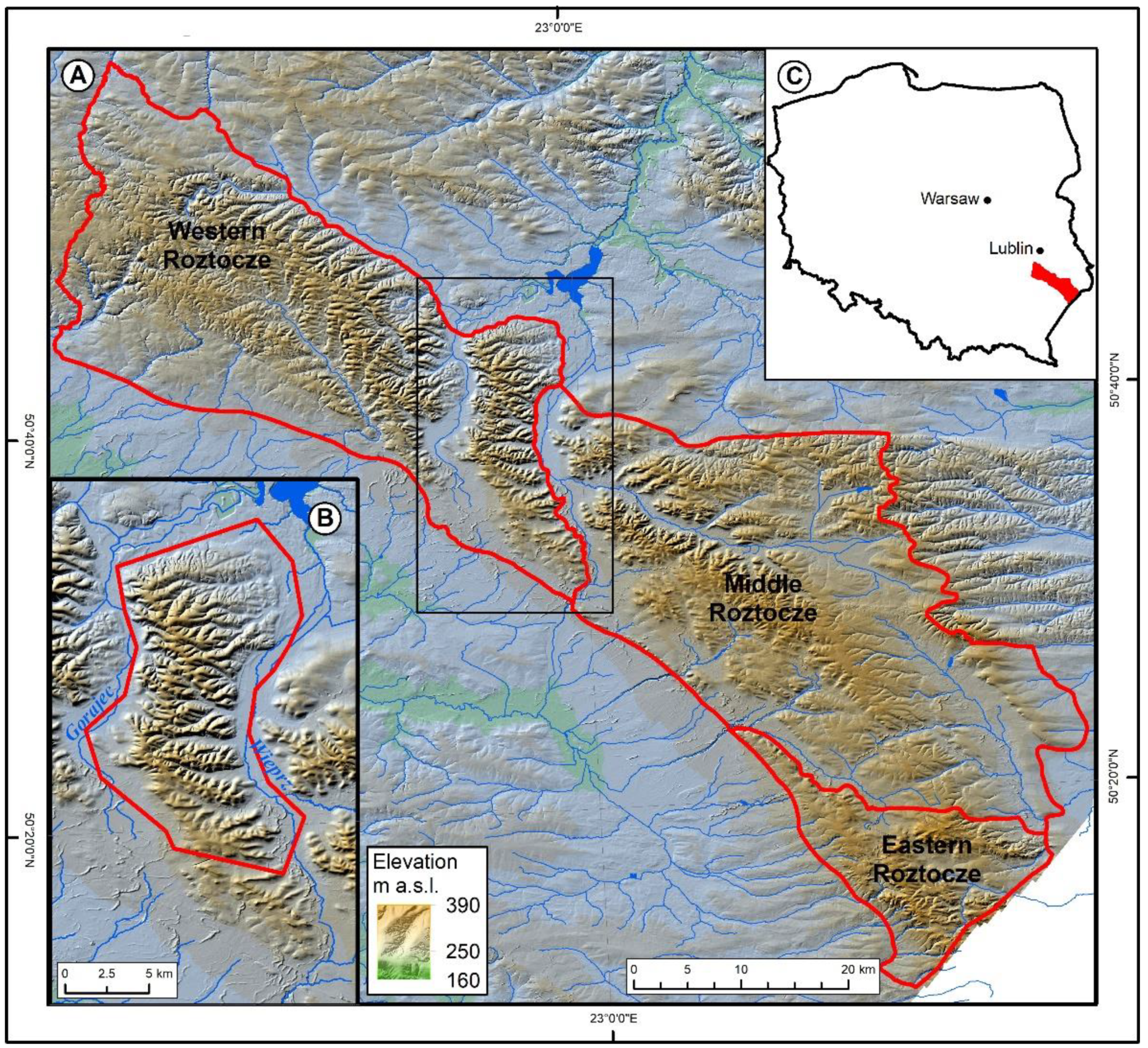
2.1. Study Area

The study area is located in the central part of the Roztocze Region (microregion) (Figure 1A) [47]. Included in the Central Polish Uplands (SE Poland; Figure 1C), this region is characterised by individual physiographic features, forming a range of hills 185 km long and varying in width from 15 to 28 km (Figure 1A). The Roztocze Region connects the Lublin Upland with the Podolia Region, and it also separates the Sandomierz Basin from the Upper Bug River Basin. The culminations of the Roztocze Region increase from 290 m above sea level (m a.s.l.) at the NW, through 350 m a.s.l. in the central part, to 380–396 m a.s.l. in the SE part. The neighbourhood of the Sandomierz Basin makes the clearly delineated SW edges of Roztocze reach heights of 50–100 m. According to Buraczynski [48], the varied orography of Roztocze predicts its division within Polish territory into four regions: Goraj Roztocze, Szczebrzeszyn Roztocze, Tomaszów Roztocze and Rawa Roztocze. Their natural boundaries are formed by the meridionally oriented valleys of the Gorajec and Wieprz rivers and the Tanew trench with the Narol-Belzec valley, splitting the Roztocze ridge into separate plateaus [48].
In the current study, Szczebrzeszyn Roztocze was analysed. In the Central Polish Uplands belt, this is the area with the highest density of valleys (mainly gullies). The subregion forms a ridge from 5 to 8 km wide and 25 km long, limited by the meridional sections of the Gorajec and Wieprz River valleys (Figure 1A). The eastern slope of the ridge is dissected by long parallel valleys. Buraczynski [49] divides the region into two blocks. The northern block, which is the subject of the study (with a N-S direction), is covered by a thicker loess cover cut through by a dense network of dry valleys and narrow loess ridges (Figure 1B). The axes of the dry valleys are dissected by a dense gully network, reaching an average density of 4.2 km/km2, with a maximum of 10.5 km/km2. Large alluvial fans have developed at the mouths of the valleys. In contrast, in the landscape of the southern block, which is mainly made up of opoches, narrow ridges of the peneplain (300–320 m above sea level), punctuated by wide valleys with a latitudinal course, stand out. Relative heights in this part are 60–70 m, with a maximum of 105 m [49] (Figure 1B).

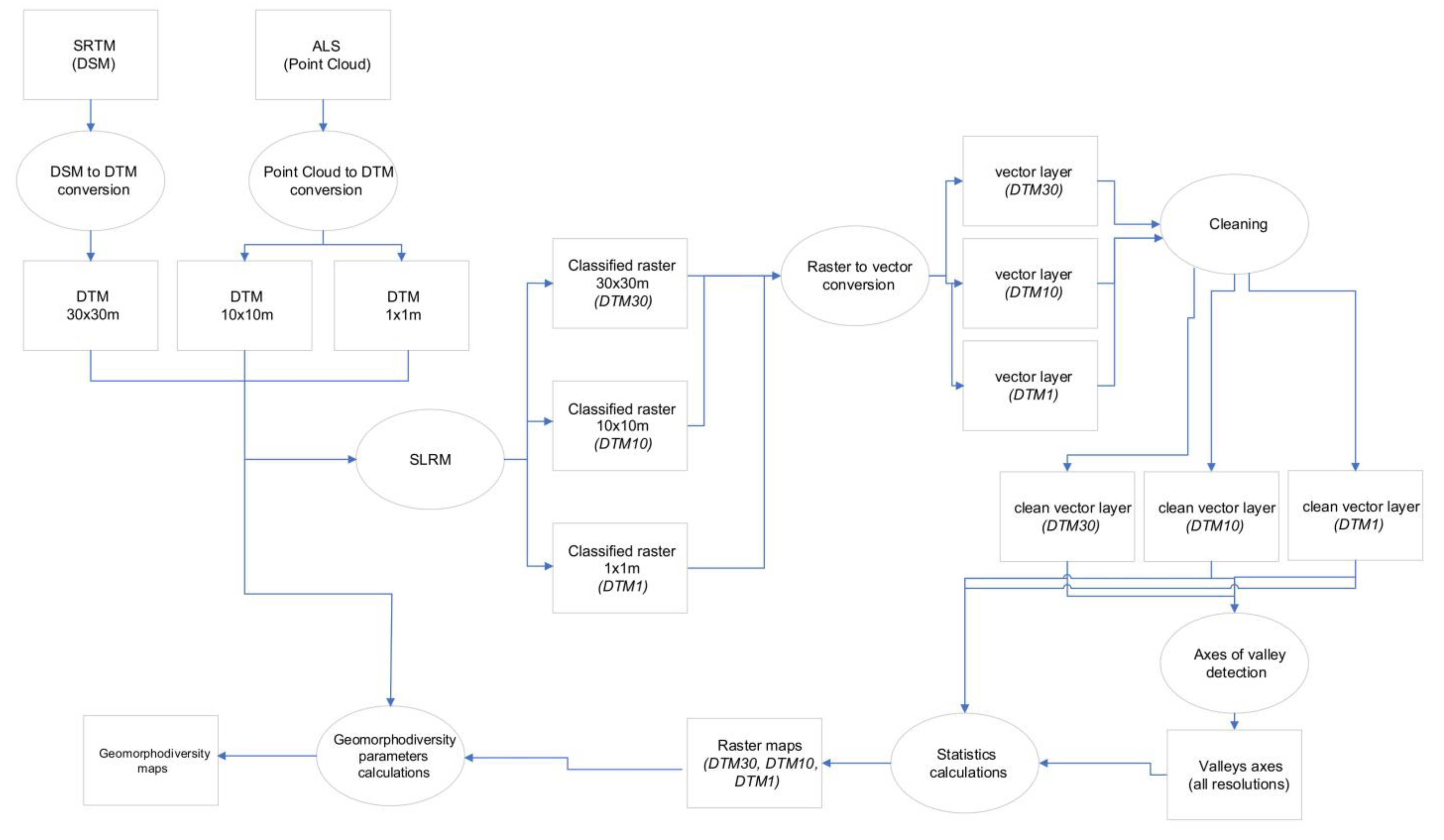
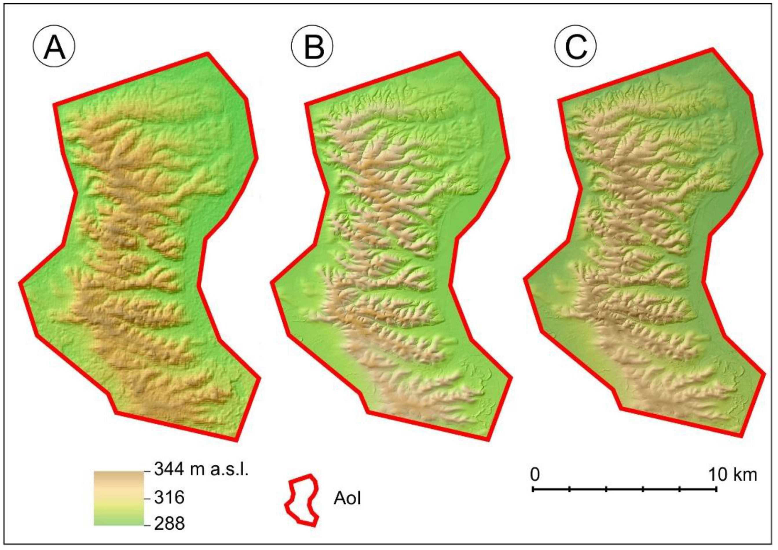
2.2. Remote Sensing Data and the Development of Numerical Terrain Models

Elevation models developed from SRTM [50] and airborne laser scanning (ALS) elevation databases were the basis for the analyses conducted. SRTM data (DSM) were obtained from the https://www.usgs.gov/centers/eros (accessed on 3 September 2022) database from the SRTM GL1 Ellipsoidal collection. These data have a spatial resolution of about 30 m, they are available for free, and they have global coverage. SRTM-derived DTM30 was obtained by converting SRTM data from the DSM model to the DTM model, using the method proposed by Zhang et al. [51] (Figure 2).
High-resolution ALS data are usually made available by the geodetic services of individual countries. In this case, the data were obtained from the Head Office of Geodesy and Cartography (GUGiK) as point clouds, classified according to the American Society for Photogrammetry and Remote Sensing (ASPRS) standard [52] and made available through the online Geoportal platform (https://www.geoportal.gov.pl (accessed on 3 September 2022). The ALS data, which are made widely available free of charge, cover more than 90% of Poland’s area, and they were acquired as part of the ISOK National Guard Information System project [46]. LiDAR point cloud density for the Szczebrzeszyn Roztocze area ranges from 4 pts/m2 to 12 pts/m2. The total number of analysed cloud points for the entire studied region is more than 1.5 billion (1,574,928,417). All acquired LiDAR elevation data were processed into DTMs layers (Figure 3) with resolutions of 10 × 10 m (DTM10) and 1 × 1 m (DTM1), using SAGA 8.3.0. software. The Channel Network and Drainage Basins module was used, based on the D8 algorithm [53]. This choice of the resolution of the DTMs used in the analyses refers to the different elevation datasets currently in use: the SRTM (which is the basis of calculated DTM30) has been available since 2001 and has global coverage; DTM10 refers to the commercial WorldDEM with a resolution of 12 × 12 m, available since 2014 (that can be easily converted to DTM); while the most accurate model (DTM1) corresponds to the DTMs developed from LiDAR data in many countries of the world.
On the basis of particular DTMs, Simple Local Relief Model (SLRM) was calculated according to the procedure proposed by Thompson [54] (Figure 2). SLRM, known as ‘trend removal’, presents the isotropic relief value in 8-bit grey scale. This enables easy separation of lower-lying areas, while removing the large-scale landscape trend [55]. SLRM was classified to extract both complex systems and individual valley forms. It was considered that the boundary values of the SLRM index should be the same for each of the input DTM. The same value of 20 cells in all cases was adopted as the trend direction search field, necessary for determining boundary areas. The threshold for the detection of valley forms (including gullies) was assumed to be a value ≤ 100 on the 8-bit scale of the algorithm used. The value was determined empirically. Objects with an SLRM index value less than or equal to 100 were classified as valley/gully forms and further analysed.

2.3. Local Relief Model (LRM)

Once the classification based on the LRM model and simple masking values above 100 (in 8-bit scale) was done, the resulting raster layer was converted to vector lines. For each DTM considered, a parameter analysis was also performed to best match both the area and the length of the landform (valley/gullies) to the relief. In addition, for each type of resolution, ‘cleaning’ of images to remove ‘artifacts’ remaining after automatic classification was performed (Figure 2). The cleaning of artifacts was performed manually, based on the course of gully edges visible on 1:10,000 scale topographic maps in the form of contour lines density or adequate signature, as well as comparison to an aerial photograph of the area with 0.25 m resolution. Valley form axes were determined for each DTMs separately, using the Module Channel Network and Drainage Basins tool in SAGA-GIS 8.3.0 software and the D8 algorithm [53]. For each of the DTMs, an appropriate threshold parameter was selected, using the expert method in order to obtain the best possible results. For DTM30, it was a value of 5th Strahler order, adopted to valley axes, while for DTM10 and DTM1, a threshold of 3rd Strahler order gave the best results. In the next step, the axes of the forms were trimmed to the boundary of the previously determined valley forms.

2.4. Calculations of Geomorphodiversity Index

It was assumed that in the case of geologically homogeneous areas, they should be treated as leading. The several morphometric parameters were also taken into account for better characterization of the relief, i.e., the number and length of valley forms, their area and volume. Unlike the first two indicators, they were not analysed directly, but in the form of derived indicators.
To assess the geomorhodiversity of homogeneous areas, e.g., loess plateaus, three morphometric indicators based on parameters of designated valley forms were calculated next:
The commonly determined, for loess areas, index of valley (gully) density, calculated as the quotient of the length of the gullies to the area of the region or basic area:
(1)
Gully Density (GD)
where: [27]
GD = L/A (m/m2) L—gully length; A—area
In addition, two new indicators have been proposed, which the authors believe enhance the assessment of geomorphodiversity:
(2)
Relative Valley Area (RVA)
where RVA = VA/A (m2/m2)
VA—valley area; A—area
and
(3)
Area-normalised Valley Cubature (AVC)
where AVC = VC/A (m3/km2)
VC—valley cubature; A—area
The dimensionless RVA index can also be expressed as a percentage (%) of the area of valley forms for a basic field of 1 km2. In turn, the AVC index shows the spatial variability of the main relief features of the analysed area.
The volume of the valleys was calculated using the Volume Calculation Tool in qgis software [56].
The geomorphodiversity index was calculated using the Weighted Sum and Zonal Statistics tools in ArcGIS. In the first step, each indicator was classified as one of five value classes of geomorphodiversity: very low, low, medium, high and very high. Next, the total indicator was calculated as the sum of the values of all the partial indicators for each 1 km2 cell (Table 1).

3. Results

3.1. Basic Parameters

The number and morphometric parameters of the separated forms are visibly influenced by the spatial resolution of the input data used (Figure 4). In terms of the number of separated valley forms and their volume, the difference between the extreme models (DTM30 and DTM1) increases in proportion to the model resolution by 10 times and almost 19 times, respectively. On the contrary, the analysis of the area shows an inverse relationship. In this case, the total area of the separated valley forms is five times smaller for DTM1 than for DTM30 (Table 2).

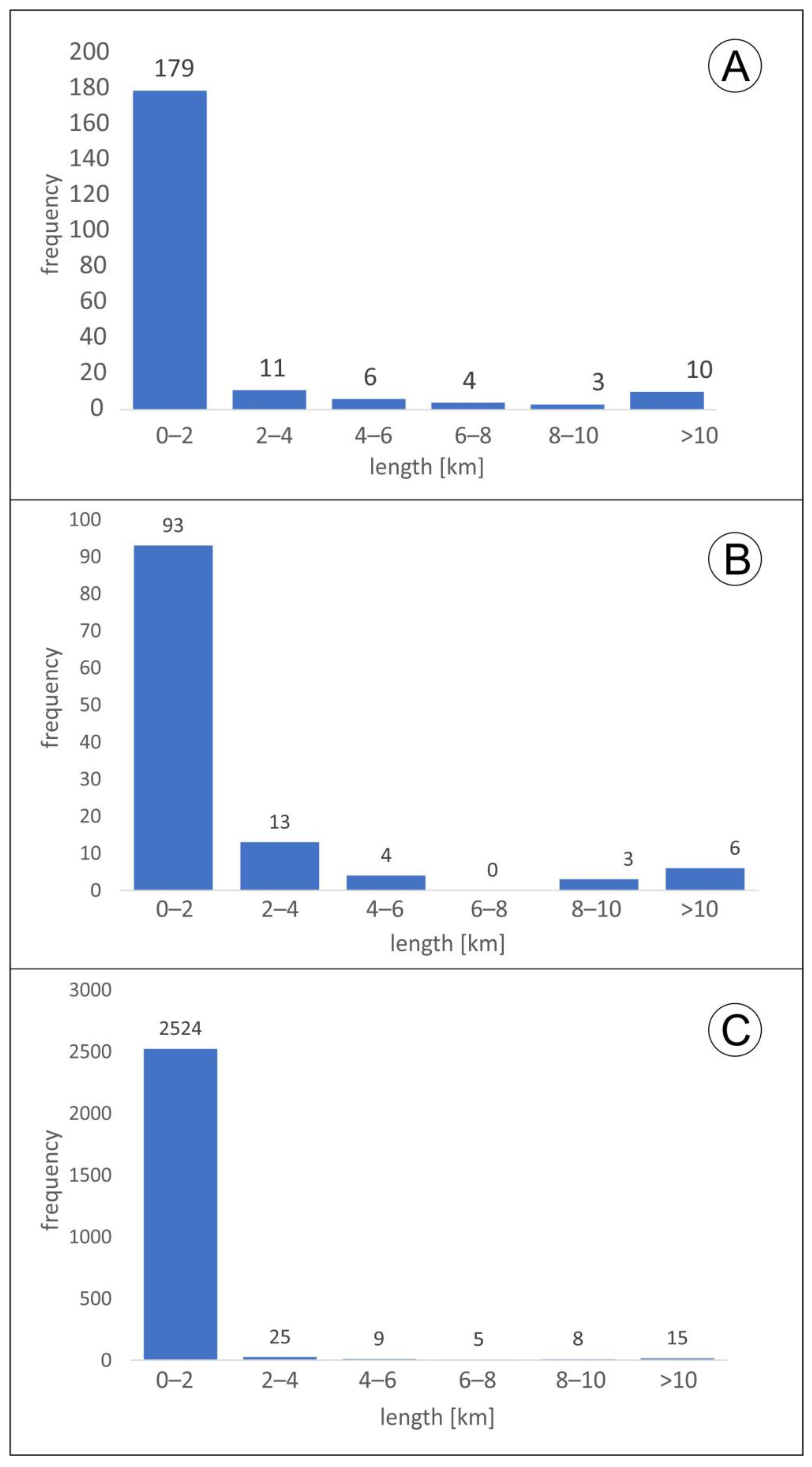
3.2. The Number and Length of the Axis of the Valley Forms

As the resolution of the basal DTM’s increases, the number of separated valley forms triples, and for DTM 30, DTM10 and DTM1 is 120, 434 and 1237, respectively (Table 1). One of the basic morphometric characteristics of valleys is their length. In this study, the axes of the valleys/gullies were determined automatically using the D8 algorithm. The largest total length of valley form axes (1975.5 km) was classified for DTM1. The sum of their lengths is almost three times higher in comparison with the DTM10 data and almost twice as high in comparison with the DTM30 data (Table 2). In each case, the longest axes of valley forms are found in the northern part of Szczebrzeszyn Roztocze. In all cases, the maximum length of the axis of the valley forms was similar and amounted to about 40 km. The highest average length of valley forms (slightly more than 2 km) is shown by forms classified as DTM10, while the lowest (about 200 m) is for DTM1. The most common forms in the analysed area are 30 m, 70 m and 320 m long for DTM1, DTM30 and DTM10, respectively (Figure 5).
In each of the examined examples, more than half of the axes are less than 1 km of length. In the SRTM-based DTM30 classification analysis, this is almost 80% of all axes, while in the case of DTM10 and DTM1, it is 65 and 95%, respectively (Figure 5). Valley system axes exceeding 10 km of length are relatively rare. The largest number of such objects (more than 5%) was classified for DTM10. The fewest valley axes exceeding 10 km in length (just 0.05%) were classified for DTM30 (Figure 5).

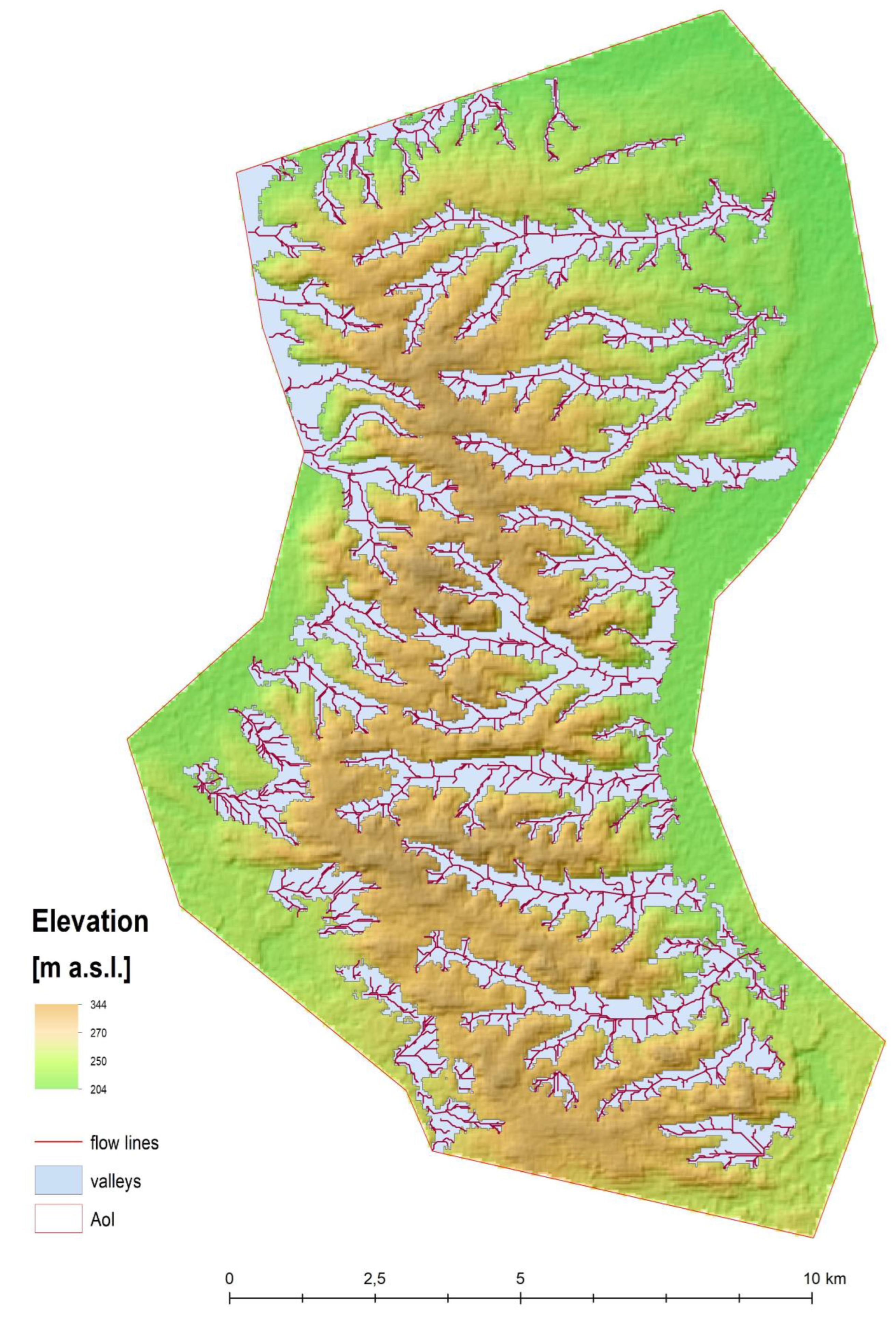
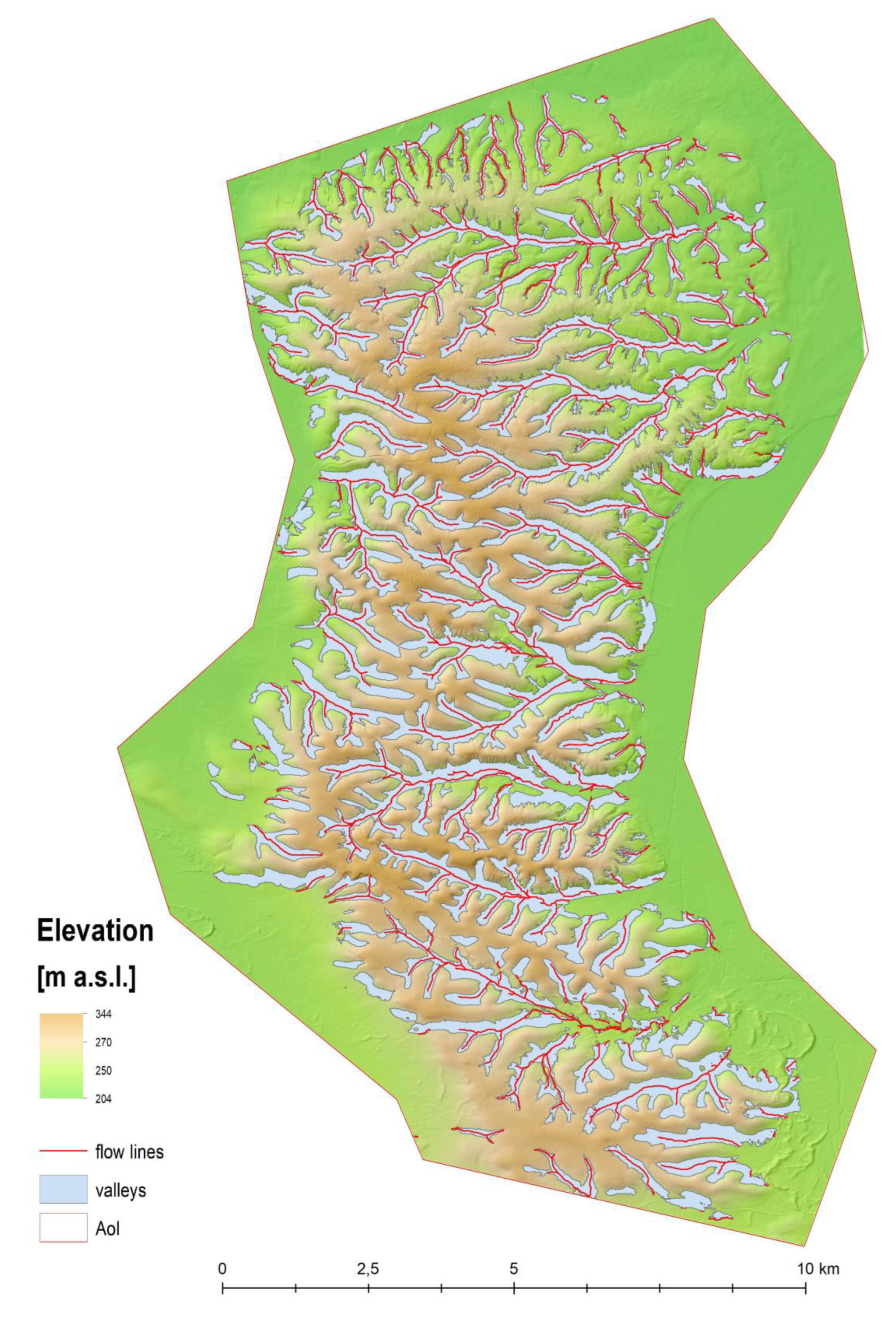
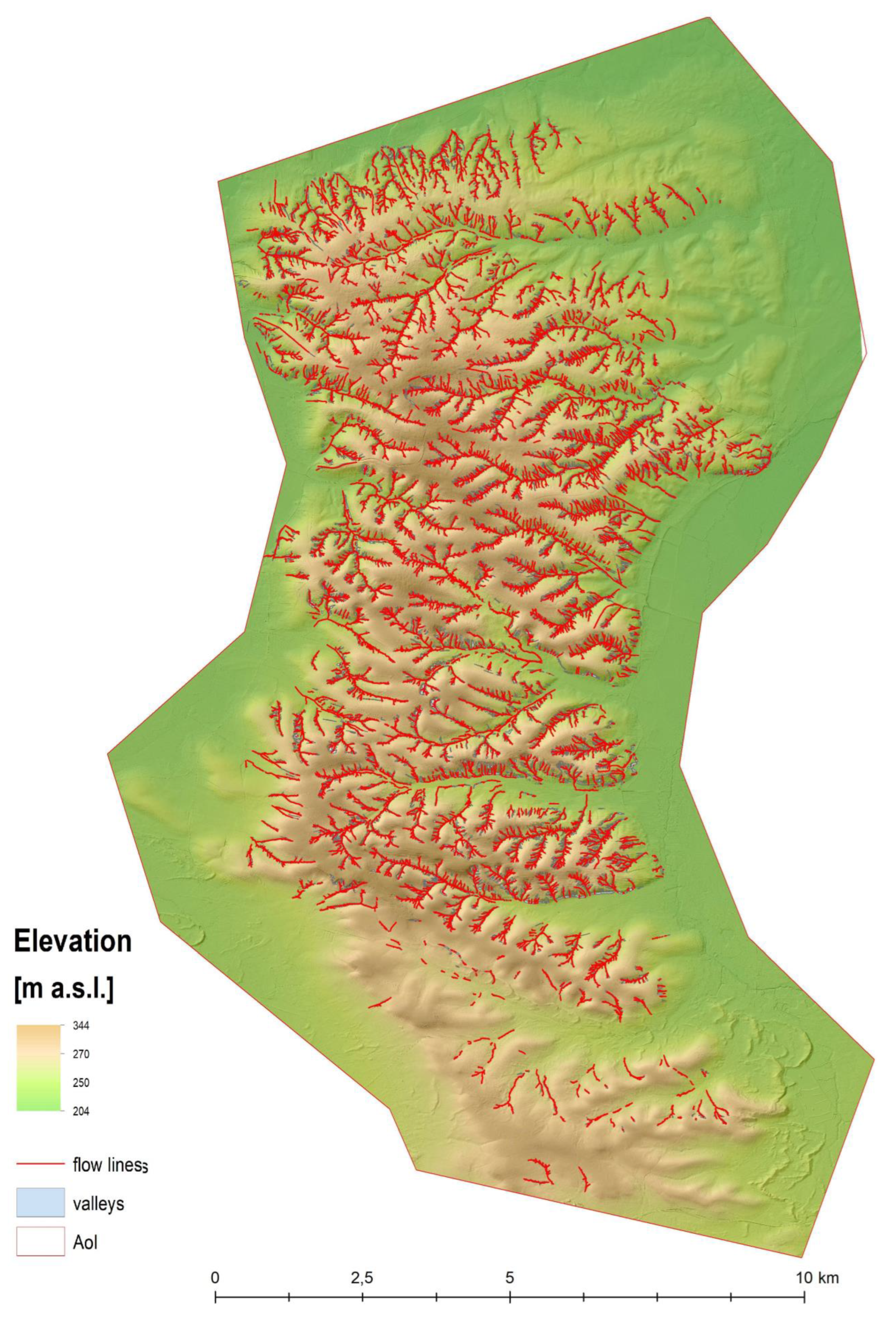
3.3. The Valley Forms/Gullies Area

For DTM30, 120 valley forms with a total area of just over 48.1 km2 have been identified. The maps presenting the DTM30 derivatives clearly show the asymmetry (W-E) of the spatial distribution of the valley forms. In the western part of the AoI, smaller and highly fragmented valley forms are observed. In contrast, the eastern part of the region is characterised by the occurrence of a larger number of highly fragmented and extensive valley systems, both in terms of the area and the length of the forms (Figure 6). The total number of valley forms (gullies) mapped on the basis of DTM10 is 434 (Table 2). The average area of a valley/gully is just over 0.1 km2, while the total area is 42 km2. The largest valley system has an area of just under 4 km2 and is located in the central part of the AoI (Figure 7).
The largest number of valley forms that were automatically classified in the AoI are characterised by DTM1 (Figure 8). In this case, 1237 objects with an average area of less than 0.01 km2 were separated (Table 2). Such a large number of objects was generated as a result of the segmentation of the large valley forms. The total area of the delineated valley forms for DTM1 is slightly more than 10 km2 and is smaller than the classified ones for DTM 10 and DTM30 by 4 times and 5 times, respectively. The valley form with the largest area, in the case of this data, occurs in the north-central part of the AoI and has an area of just over 0.5 km2 (Table 2).

3.4. Volume of Valley Form/Gullies

The highest total volume of valley forms of 1,058,032,348 m3 was obtained for DTM10 (Table 2). Lower values were obtained from the analyses of DTM1 (1,027,728,663 m3) and DTM30 (13,148,538 m3). The average volume of valley forms within the analysis area ranged from 109,571 m3 (DTM30) to just over 251,937 m3 (DTM10). The average volume of the valley form/village for DTM1 and DTM10 in the analysis area was about 470 m3. The smallest valley forms analysed in the area range in volume from less than 1 m3 (DTM30) to more than 60 m3 (DTM10) (Table 1).

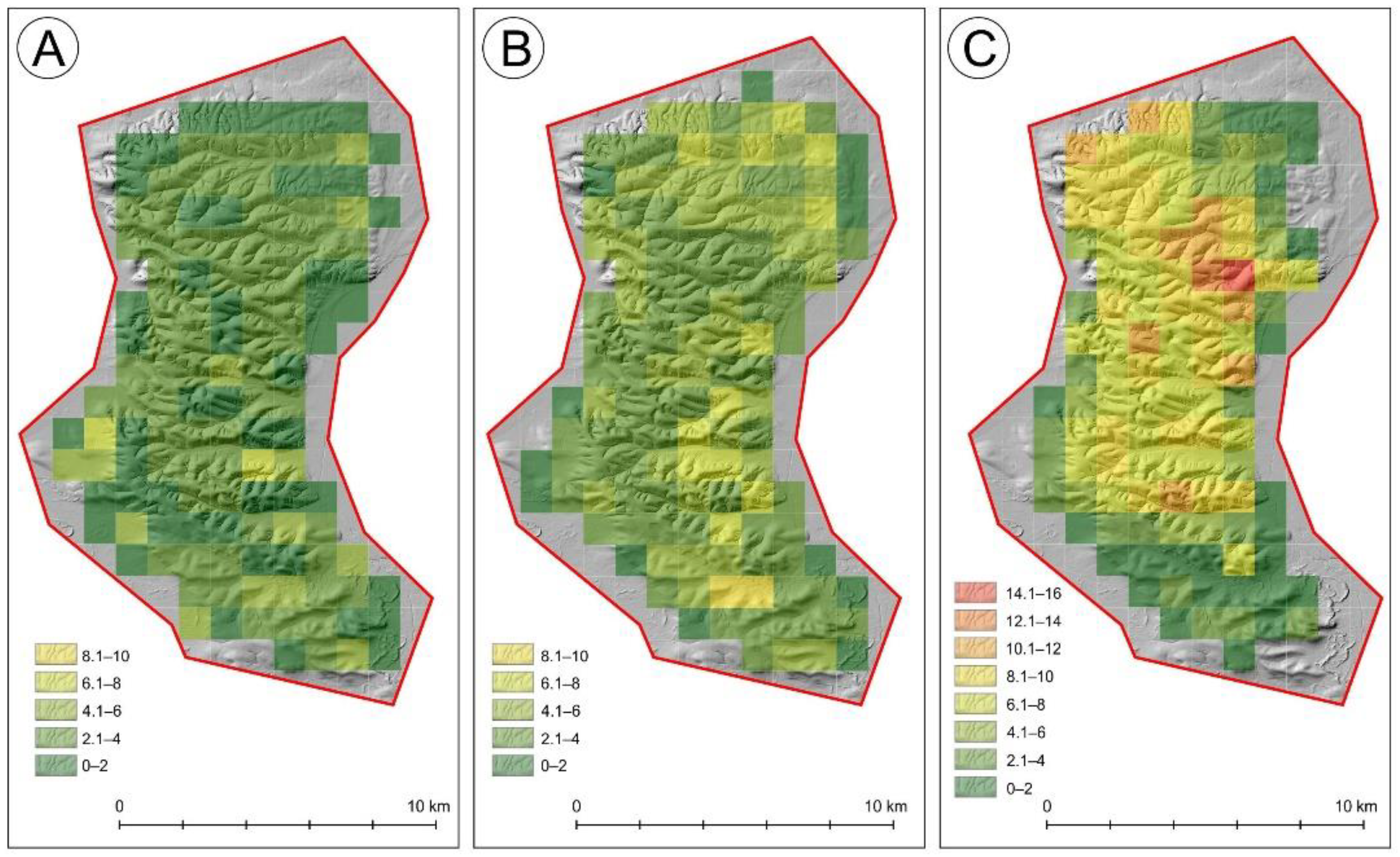
3.5. Density of Valley Forms/Gullies (GD)

For geologically homogeneous areas, basic morphometry analysis can be supplemented by complex indicators derived from the basic parameters previously described. The first and most commonly used in the analysis of the relief of loess areas is the density of valley forms (gullies) (GD). The average value of this parameter in the analysed area is more than 5 km/km2 for DTM1, while for DTM30 and DTM10 it is much lower, even 2 times lower in the case from DTM30. The highest maximum value of the density of valley forms is characterised by DTM1 (Table 3). The estimated density of gullies corresponds well with data from the literature for the study area, where the calculated values of this parameter were in a similar range, although they reached slightly different maximum values [25].
The resolution of the source model also determines the spatial distribution of valley form density (Figure 9). For DTM30, the highest density of forms (more than 5 km/km2) occurs in the southern and central parts of the analysis area. For DTM10, the highest densities (about 3 km/km2) occur in the northern and eastern parts. In contrast, for DTM1, the density of gullies increases, from S to N, from less than 1 km/km2 to more than 10 km/km2. The recorded spatial variability of the analysed indicator is probably related to the accuracy of the algorithm used to separate gully forms, which is closely linked to the spatial resolution of the input data.

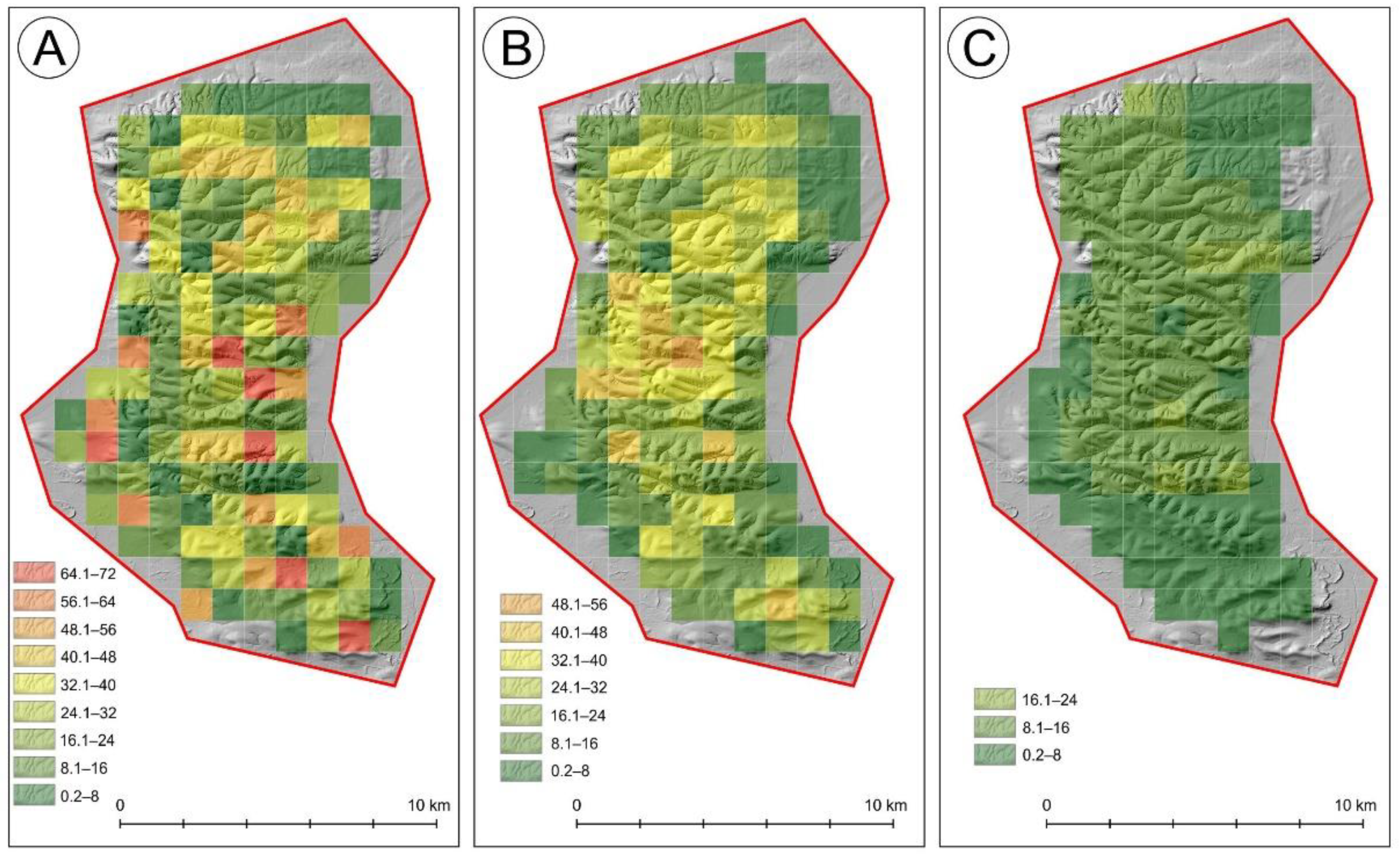
3.6. Relative Valley Area (RVA)

Another indicator proposed is Relative Valley Area (RVA). The lowest average values of the RVA index (about 8%) characterise DTM1, while the highest (nearly 25%) characterise DTM30. The difference in the average value of the RVA index between DTM30 and DTM10 is small (Table 4). The differences between the models are related to the greater generalisation of the extent of the separated gully formations in the case of lower-resolution input data.
The spatial distribution of RVA is also different for models with different resolutions (Figure 10). For ALS-derived DTM10 and DTM1, higher RVA values are found in the central part of the analysed area. SRTM-derived DTM30 shows dispersion of RVA values. Their spatial distribution is a mosaic of different neighbouring classes, without clear areas of concentration. It can be concluded that as the spatial resolution of the classified material decreases, the value of the RAV index increases. Most of the valley forms in the AoI are less than 0.1 km2 in area. For DTM1-designated sites, valley forms with an area greater than 0.1 km2 account for only 1.5% of all classified sites. For DTM10, such sites account for almost 17%, and for DTM30, more than 21%. This shows that during the classification of DTMs with higher spatial resolution, many more valley forms with smaller areas are separated than in the case of low-resolution elevation models. The achieved classification results also indicate that as the spatial resolution of the base model on which the automatic classification is performed increases, the total area of valley forms decreases, which may indicate a more accurate separation of these landforms.

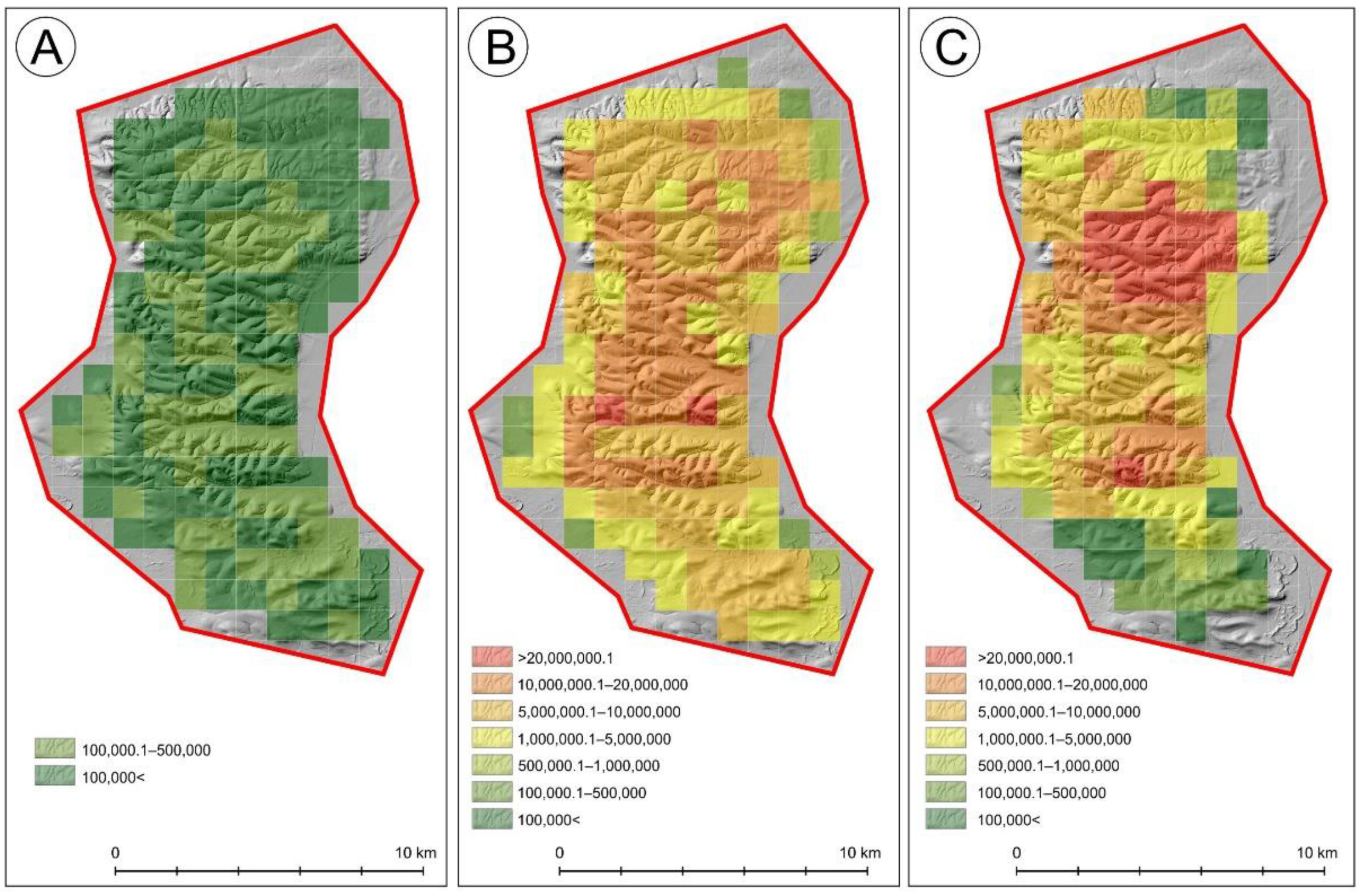
3.7. Area-Normalised Valley Cubature (AVC)

As in the case of the RVA index, the greatest variability in gully volume per unit area is found in the data calculated from the DTM30 model (Table 5; Figure 11). In contrast, the spatial distribution on LiDAR-derived DTMs shows a concentration of areas with similar AVC index values. In the case of DTM10, the highest values of volume per km2 occur in the central part of the analysed area, while in the case of DTM1, the area with the highest index values appears more towards the north, compared to the DTM10 data (Figure 11).

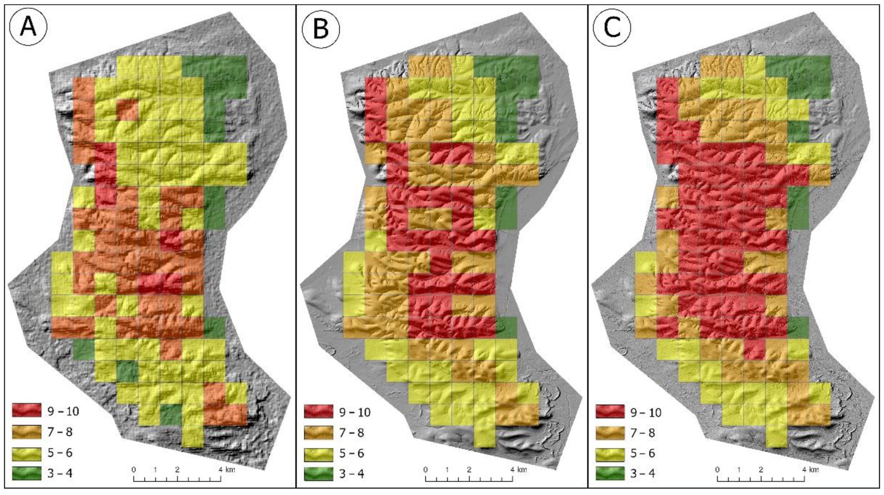
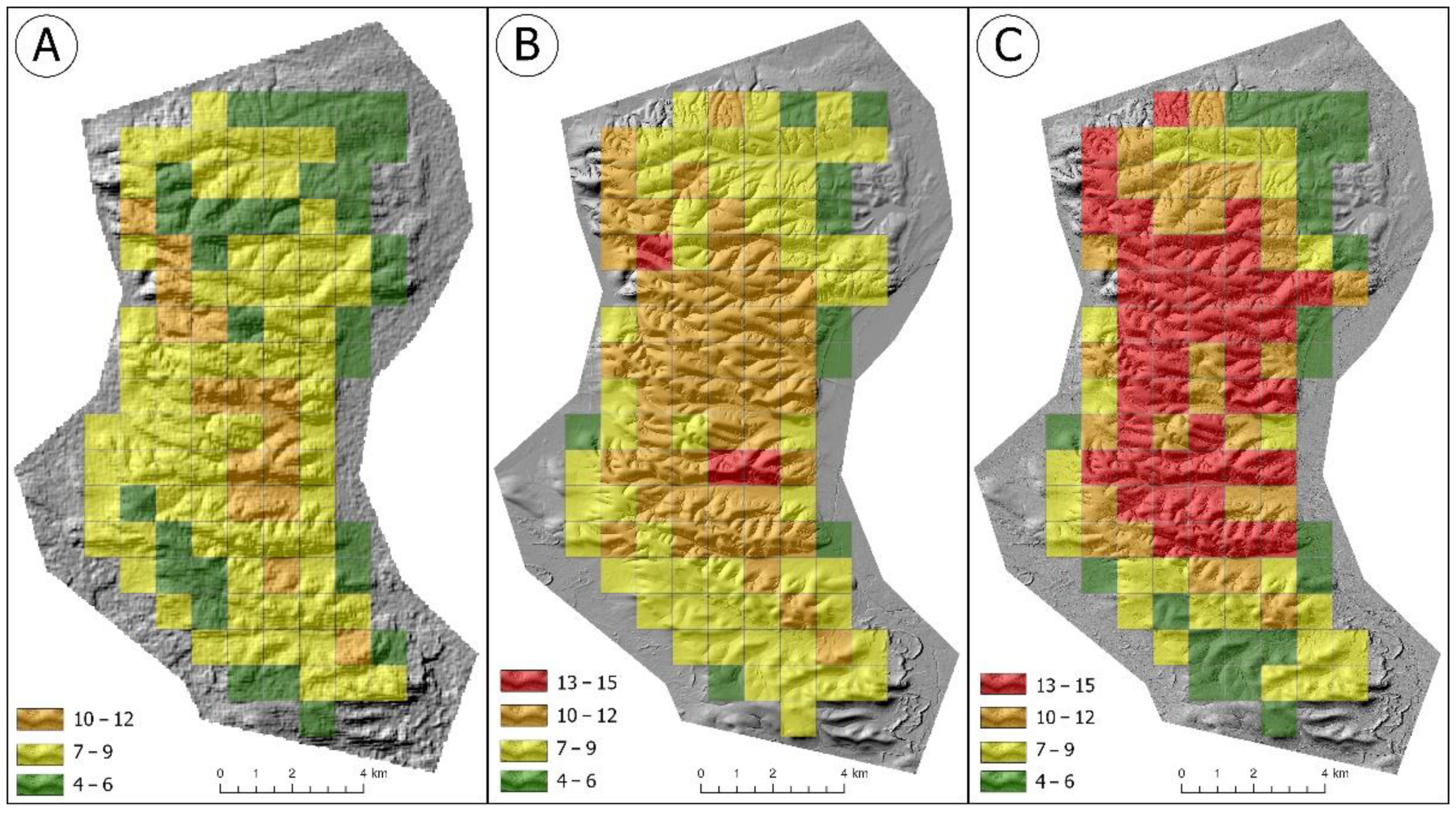
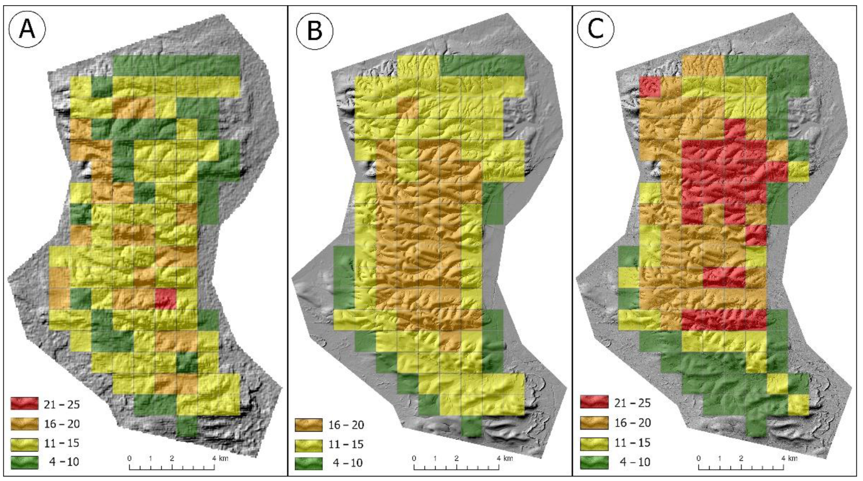
3.8. Index of Geomorphodiversity

Finally, the index of geomorphodiversity was calculated based on two (Figure 12), three (Figure 13) and five (Figure 14) factors, using 1 km2 squares, according to Table 1. It was done in that way to better visualise homogeneous spatial units. In this way, we show how the spatial pattern of the total index changes due to invented, partial indices.
The spatial pattern of the geomorphodiversity index based on relative heights and slope is different for each DTM, but some similarities can be observed. The lowest values (class 3–4) occur on the outside zone of the AoI, most located in the NE part. The second class (5–6) occupies the largest area on DTM30 (Figure 12A) and is located in the northern and southern parts of the AoI. On DTM10 and DTM1, it occupies the smallest areas, in the same locations as on DTM30. The third class (7–8) occupies the largest area on DTM30, located mainly in the central part. On DTM10 and DTM1, it also occupies the central parts, but on DTM10, it is mostly spread. The highest class (9–10) occupies the largest area on DTM1, located in the central part of the AoI. On DTM10, the third class is significantly smallest and is not so compacted. On DTM30, it occurs in the central part, but it is only in a few square areas located in three places.
The spatial pattern of index calculated on three factors (Figure 13) shows some similarity to the previous case (Figure 12). The lowest class (4–6) occupies the biggest area on DTM30 and is located mainly in the outer NE and S zones, but some squares appear inside the AoI. On DTM10, the first class occupies the smallest area, located in the outside zone. On DTM1, the lowest class appears in the outside NE and S zones, similar to DTM10. The second class (7–9) occupies the biggest area on DTM30, located inside of the AoI, while on DTM10, the area of this class is smaller and is located in the N and S parts. On DTM1, the second class occupies the smallest areas and is located in the neighborhood of the first class. The third class occupies small areas in the central part of DTM30, forming a zone in a NW–SE direction. On DTM10, this class occupies a big area, located in the central part. On DTM1, the third class is not compact, and squares are located in the neighborhood of the second class. The highest class does not appear on DTM30, and on DTM10 there are only three squares, but on DTM1, it is a big area located in the central part and partly divided by the third class.
The spatial pattern of index calculated on five factors (Figure 14) shows the same regularities as the indices described above (Figure 12 and Figure 13). The lowest class (4–10) occurs mainly in the outer zone on DTM30, but some squares are inside the AoI. On DTM10, this class occupies the smallest areas located in the outer zone, and on DTM1, this class has a bigger area and is also located outside. The second class (11–15) dominates on DTM30, but it is not compact and is split by other classes. On DTM10, the second class forms the inner zone and surrounds the central part. On DTM1, this occupies the smallest area located in the neighbourhood of the first class. The third class (16–20) is strongly dispersed on DTM30, but on DTM10, it forms a compacted zone in the central part. On DTM1, this class occupies the central part and is divided by the squares of the highest class. The fourth class appears only in one square on DTM30 and is absent on DTM10, but on DTM1, it occupies the biggest areas, located in the central part.
Analyzing all the maps (Figure 12, Figure 13 and Figure 14), we can observe several correctness in spatial patterns of geomorphodiversity indices. The first (lowest) class of values is usually located in outside zones, especially in NE and S parts of the AoI, but not always (Figure 12B,C). The second class usually surrounds the central part and has strongly differentiated areas, from large (Figure 12A, Figure 13A and Figure 14A,B) to small (Figure 14C). The compactness of this class is differentiated, too, from strong (Figure 14B) to low (Figure 14B). The third class is compact only on two maps (Figure 13B and Figure 14B), and it is mixed with other classes on most of the maps. The fourth class forms clear “islands” on maps based on DTM1 (Figure 12C, Figure 13C and Figure 14C). On other maps, it is clearly marked only on Figure 12B, and occurs occasionally on Figure 12A, Figure 13B and Figure 14A.

4. Discussion

4.1. The Role of Indicators in Assessing the Geodiversity of Geologically Homogeneous Areas

Methods for quantitative assessment of geodiversity have been continuously developed and improved for almost three decades [7,8,9,10,11,12,13]. With the widening availability of environmental data, including remotely sensed satellite- and LiDAR-derived data, opportunities for a more complete characterisation of the qualities of the study area are emerging. In the geological concept proposed by Sharples [1], a key factor in determining the geodiversity of a studied area was the geological structure and, in particular, the bedrock formation diversity. In this context, it becomes problematic to assess homogeneous areas in this respect, e.g., loess plateaus, where thicker loess deposits effectively mask the diversity of deeper rocks and geological structures [57,58]. In spite of the presence of homogeneous bedrock, these areas may be characterised by high differentiation of relief, reflected either by diversification of landforms or aggregation of one type of landforms, e.g., valleys or gullies. Parameterisation of morphometric features of these forms may contribute to a more objective evaluation of the geodiversity of these areas. Thus, in the case of calculating the index strictly on the basis of morphometric parameters, we should talk about geomorphodiversity. To fulfil this condition, the delimitation of valleys should be carried out according to standardised criteria and in an automatic way. In this study, automatic delimitation of the course and extent of valley forms and categorisation of watercourses was used [59,60,61]. However, due to the impossibility of controlling the effects during the operation of the algorithm, manual verification of the classification results was necessary. The approval of appropriate cut-off values for the individual components of the classification algorithm is extremely important, as errors arising during the automation of the classification process of specific forms prevent the correct interpretation of the results [62,63]. This approach allows the inclusion of valley network parameters as additional indicators to enrich the geodiversity indices used so far [64,65,66,67,68,69]. Previous methods of analysing the spatial variability of the valley (gully) network are quite weak and mainly use an index, such as valley/gully density [70,71,72], that describes the relationship between the total length of valley forms and the area of the study area. This study proposed two new indicators that could be implemented as components of geomorphodiversity indices. The first is Relative Valley Area (RVA), which describes the proportion of the gully area in the adopted base field. It could be presented as a dimensionless index or as a percentage share. The graphical representation of the RVA indicator on the map allows a quick and correct perception of the regional variation of areas with a high share of valley form areas (Figure 10). The second proposed indicator is the Area-normalised Valley Cubature (AVC), which, by representing the relationship between the volume of valley forms and the area of the analysed area, reflects the dynamic nature of the main relief features (Figure 11). Previous studies realised in this area [25] were focused only on the volume of gullies. They are only a part of so called ’dry’ valleys in this area, usually dissecting the bottoms only of some of the bigger valley forms. The calculated AVC index [27] shows that gullies constitute only a small part of the valleys taken into account in this study.

4.2. Application of Different Resolution Digital Elevation Data to Create DTMs

Since the 1970s, studies on the use of elevation data with different resolutions have been reported [73,74,75,76,77,78]. The authors emphasise that the use of data with different spatial resolution may cause differences in the results obtained [79,80]. DEMs with low spatial resolution, e.g., SRTM, Aster, or Copernicus, are the most commonly used. Although the resolution of these data is low (in the range of 20 to 30 m), they have the advantages of free access and ease of acquisition. The advantages of this type of data is its global coverage and small file sizes that allow calculations and analyses to be performed quickly [81]. Unfortunately, the disadvantage is the low accuracy. Very often, the information developed from this data is too generalised and the classified forms too generalised [81,82]. High-resolution LiDAR-derived DTMs are much more geometrically accurate [83]. For this region-scale study, the resolution of the DTMs used for the analyses was set at 10 × 10 m and 1 × 1 m. Such high resolution data allow the extent of individual landforms, and even land use, to be determined with a high precision [84]. However, due to the relatively small spatial coverage of LiDAR data worldwide, the possibilities for its use are limited [85]. The use of LiDAR-derived DTMs also requires greater software skills to process the raw data than is the case with SRTM-derived DTMs. It also engages significantly more computer resources (computing power) in the processing [86].

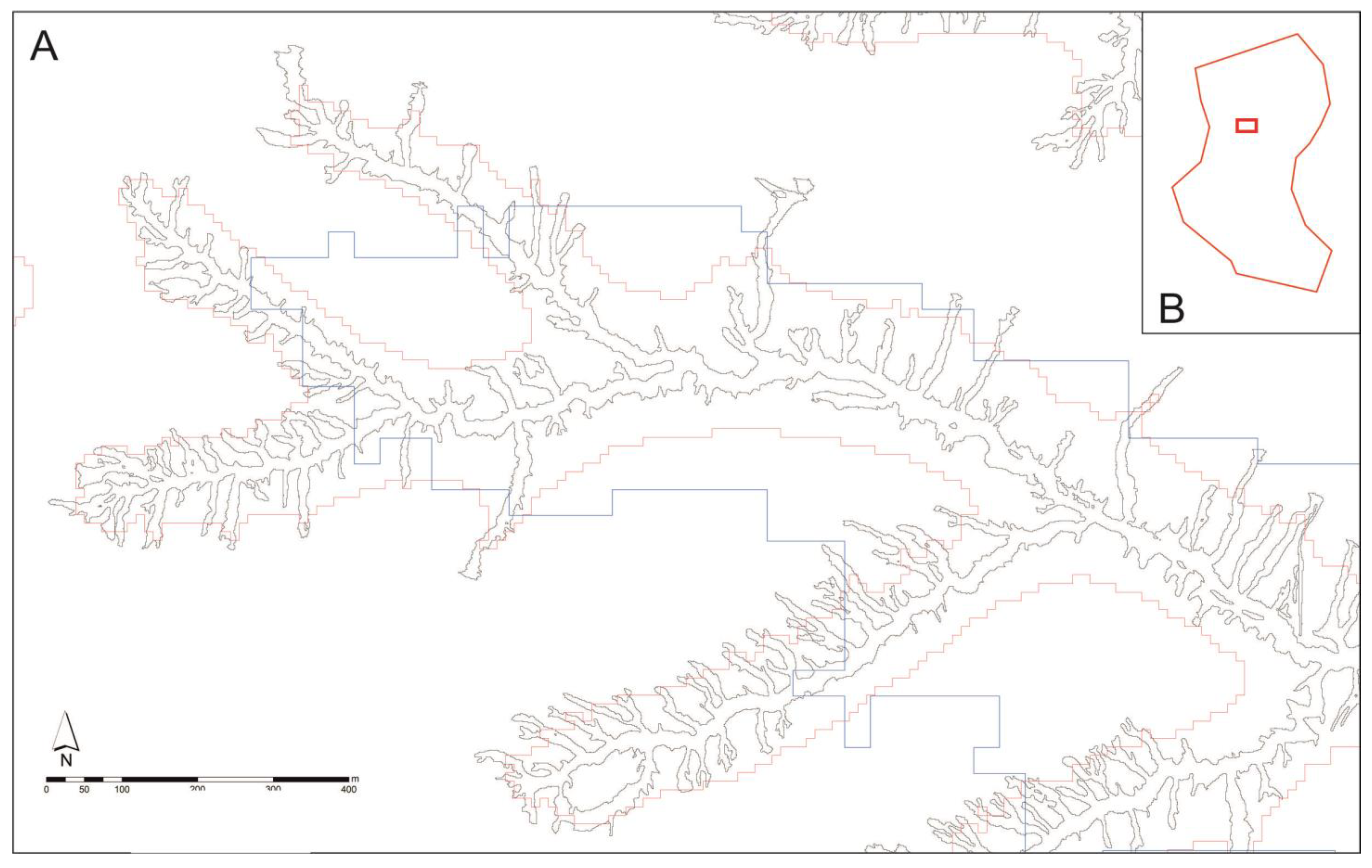
4.3. Accuracy of Delineation of Small Erosion Forms

The use of data with different spatial resolutions to delineate landforms has positive, as well as negative consequences. Precise determination of the extent and course (edge areas) of erosional landforms is difficult, even during direct mapping in the field using expert knowledge [87]. Defining such boundaries using GIS tools and quality data is definitely more precise and devoid of subjectivity [88]. The use of low-resolution spatial data can cause errors based on ambiguities related to the interpretation of elevation models. In the process of creating low-resolution DTMs, small landforms (e.g., gully branches) become ‘blurred’ [89,90]. As shown in this study with small landforms (e.g., loess gullies) whose widths are often below spatial resolution, their representation in the DTM model and analyses is skewed, or even ignored. Only large-scale forms have a chance of being correctly detected and imaged. In addition, with low-resolution data, the sheer size of the cell (base cell) can result in a variation of the form edges, which can consequently over- or underestimate the area of specific forms. The use of SRTM data to create DTMs is very common. Using them, however, requires processing from the raw data representing the DSM to form a DTM. For undeveloped areas covered by low vegetation, this type of processing is relatively straightforward, while the largest errors occur in areas covered by forests and urbanised areas [49]. For analyses related to valley formations, the use of SRTM-derived DTM data is limited by the low spatial resolution (30 m). However, such low-resolution models are in some cases the only source of elevation information [91,92]. The analysis of individual morphometric parameters of separated valley forms showed clear differences of several, or even a dozen, times, depending on the resolution of the model. Large differences in the volume of valley forms may result from an increase in the generalisation of the shape of concave forms occurring with a decrease in the resolution of the terrain model, on the basis of which the volume estimate was made [93,94]. Landforms that are less than cell size are obscured in lower-resolution models. It is sufficient that only one of the parameters ,the width of the valley floor, is smaller than the side of the cell, the entire valley form is incorrectly imaged on the model. In addition, analyses based on lower-resolution DTMs do not take into account the variability of the bottom of the individual valley landform [95,96].

4.4. Possibilities of Using High-Resolution Elevation Data and Limitations Associated with the Use of These Data for Large Areas

Acquiring and processing high-resolution spatial data is costly and time-consuming. Depending on the measurement technology used, high-resolution spatial data are often only acquired for small areas [97]. In the case of remote sensing techniques, data acquisition usually takes from several minutes (UAV photogrammetry, ALS) to several hours (TLS). On the other hand, processing the data into DTM, depending on hardware and software resources, can take from several minutes to several hours [98,99]. The relatively small amount of work involved in acquiring and processing this type of data from a small area (up to 2–3 km2) creates opportunities for analyses with higher resolution. Extrapolating this type of information to larger areas is not straightforward and remains a significant difficulty for many researchers [98]. The results of regional-scale analyses, however, show that the use of high-resolution ALS-derived DTMs give a much better depiction of the geomorphodiversity of an area than low-resolution SRTM-derived DTMs.

5. Conclusions

This study was carried out for the Szczebrzeszyn Roztocze, one of the most landscape-diverse loess regions in Poland. The analysis covered an area of 176 km2, almost homogenous in geological terms (loess dominance). A distinctive feature of this region is a high concentration of gullies, the density of which exceeds 10 km/km2. It was shown that for this type of area, homogeneous in terms of bedrock, the evaluation of geomorphodiversity can be enriched by parameters related to the dominant network of dry valleys and gullies in the landscape. It was also shown that the computational process can be largely automated by relying on digital terrain models (DTMs) and algorithms for automatic delimitation of borders and axes of valley forms.
Selective analyses of topographic texture were performed for three elevation models of different origin and resolution, viz: SRTM-derived DTM 30 m and two ALS-derived DTMs of 10 m and 1 m. It was shown that the use of the Simple Local Relief Model (SLRM) algorithm for the delimitation of valleys and gullies gives better results for models with better resolution (DTMs 10 m and 1 m). SRTM-derived DTM30 (by 30 m cell) results in an over-generalisation of the shape of the valleys. The shape and course of most gullies, which are generally less than 30 m wide, were incorrectly delineated or omitted and, thus, the indices calculated from this source have the largest range of uncertainty.
In addition to the inclusion of quantitative parameters of erosional landforms, such as the number, length, area and volume of landforms in the quantitative evaluation of the geomorphodiversity of loess areas obtained from topographic texture analyses, the authors propose to enrich the list of indicators used with the density of valleys/gullies, the degree of ‘coverage’ of the area by valley landforms or the ‘degree of erosivity’. In addition to the gully density (GD) indicator generally used in loess area morphometry, two new indicators are proposed. Relative Valley Area (RVA) is a dimensionless index of the proportion of valley landforms in a basal area of 1 km2 (it can also be expressed as a percentage %). Area-normalised Valley Cubature (AVC) is an indicator showing the amount of removed (eroded) sediment relative to the valley area, while also showing the dynamic nature of the main relief features of the study area.
The index of geomorphodiversity calculated with the use of new indicators allows looking at this problem with richer knowledge of relief, including the third dimension. It broadens the way we understand geomorphodiversity and shows the problem in a more complete way.
The results of this study further show that the accuracy of the delineation of valley/valley boundaries increases with the decrease of the size of the DTM’s cells. Automated topographic texture analysis allows delimitation and extraction, as well as statistical analysis of the parameters of gullies, but the resolution of the source model must be matched to the nature and parameters of the leading relief landforms of the analysed area.

Supplementary Materials

The following supporting information can be downloaded at: https://www.mdpi.com/article/10.3390/resources12010007/s1. Figure S1. Digital Terrain Models derived from various sources of elevation data: (A) DTM30; (B) DTM10; (C) DTM1.; Figure S2. Spatial variability of valley forms/gullies density derived from various sources of elevation data: (A) DTM30; (B) DTM10; (C) DTM1.; Figure S3. Spatial variability of the amount of RVA derived from various sources of elevation data: (A) DTM30; (B) DTM10; (C) DTM1.; Figure S4. Spatial variability of the amount of AVC derived from various sources of elevation data: (A) DTM30; (B) DTM10; (C) DTM1.

Author Contributions

Conceptualization, M.S. and W.K.; methodology, M.S. and W.K.; software, M.S. and L.G.; data curation and calculations, M.S.; writing—original draft preparation, M.S., W.K. and L.G.; editing, M.S., W.K., L.G. and P.B.; visualization, M.S., L.G. and P.B. All authors have read and agreed to the published version of the manuscript.

Funding

This research received no external funding.

Institutional Review Board Statement

Not applicable.

Informed Consent Statement

Not applicable.

Data Availability Statement

The data presented in this study are available on request from the corresponding author.

Acknowledgments

The authors would like to thank the Reviewers for their valuable comments that helped to make the improvements that were essential to the successful completion of this work. The authors are also grateful for the English language proofreading by Andrew Warchoł.

Conflicts of Interest

The authors declare no conflict of interest.

References

  1. Sharples, C. A Methodology for the Identification of Significant Landforms and Geological Sites for Geoconservation Purposes; Forestry Commission Tasmania: Hobart, Australia, 1993. [Google Scholar]
  2. Sharples, C. Geoconservation in Forest Management-Principles and Procedures. Tasforests-Hobart 1995, 7, 37–50. [Google Scholar]
  3. Kiernan, K. An Atlas of Tasmanian Karst: Volumes 1–2; Tasmanian Forest Research Council Inc.: Hobart, Australia, 1995. [Google Scholar]
  4. Dixon, G. Geoconservation—An International Review and Strategy for Tasmania; Parks and Wildlife Service: Hobart, Australia, 1996. [Google Scholar]
  5. Eberhard, R. Pattern & Process: Towards a Regional Approach for National Estate Assessment of Geodiversity: Report of a Workshop Held at the Australian Heritage Commission on 26 July 1996; Environment Australia: Canberra, Australia, 1997; ISBN 978-0-642-27014-6. [Google Scholar]
  6. Sharples, C. Concepts and Principles of Geoconservation; Tasmanian Parks & Wildlife Service: Hobart, Australia, 2002. [Google Scholar]
  7. Gray, M. Geodiversity: Developing the paradigm. Proc. Geol. Assoc. 2008, 119, 287–298. [Google Scholar] [CrossRef]
  8. Gray, M. Geodiversity, geoheritage and geoconservation for society. Int. J. Geoheritage Park. 2019, 7, 226–236. [Google Scholar] [CrossRef]
  9. Kozłowski, S. Postępy prac nad ochroną georóżnorodności w Polsce. Kosmos 2001, 50, 151–165. [Google Scholar]
  10. Kozłowski, S. Geodiversity. The concept and scope of geodiversity. Przegląd Geol. 2004, 52, 833–837. [Google Scholar]
  11. Serrano, E.; Ruiz-Flaño, P. Geodiversity: A theoretical and applied concept. Geogr. Helv. 2007, 62, 140–147. [Google Scholar] [CrossRef]
  12. Pellitero, R.; Manosso, F.C.; Serrano, E. Mid- and large-scale geodiversity calculation in fuentes carrionas (nw spain) and serra do cadeado (paraná, brazil): Methodology and application for land management. Geogr. Ann. Ser. A Phys. Geogr. 2015, 97, 219–235. [Google Scholar] [CrossRef]
  13. Reynard, E.; Giusti, C. The Landscape and the Cultural Value of Geoheritage. In Geoheritatge: Assessment, Protection and Management; Brilha, J., Reynard, E., Eds.; Elsevier: Amsterdam, The Netherlands, 2018; pp. 27–52. ISBN 978-0-12-809531-7. [Google Scholar]
  14. Pereira, D.I.; Pereira, P.; Brilha, J.; Santos, L. Geodiversity Assessment of Paraná State (Brazil): An Innovative Approach. Environ. Manag. 2013, 52, 541–552. [Google Scholar] [CrossRef] [PubMed] [Green Version]
  15. Manosso, F.C.; De Nóbrega, M.T. Calculation of Geodiversity from Landscape Units of the Cadeado Range Region in Paraná, Brazil. Geoheritage 2015, 8, 189–199. [Google Scholar] [CrossRef]
  16. Maruszczak, H. Zróżnicowanie stratygraficzne lessów polskich. Podstawowe profile lessów w Polsce. UMCS 1991, 1, 13–35. [Google Scholar]
  17. Maruszczak, H. Charakterystyczne formy rzeźby obszarów lessowych Wyżyny Lubelskiej. Czas. Geogr. 1958, 26, 335–353. [Google Scholar]
  18. Maruszczak, H. Le Relief Des Terrains de Loess Le Plateau de Lublin. Ann. UMCS Sec. B 1961, 15, 93–122. [Google Scholar]
  19. Maruszczak, H. Erozja wąwozowa we wschodniej części pasa wyżyn południowopolskich. Zesz. Probl. Postępów Nauk Rol. 1973, 151, 15–30. [Google Scholar]
  20. Buraczyński, J. Erozja wąwozowa na Roztoczu—międzyrzecze Gorajca i Wieprza. Folia Soc. Sci. Lub. 1975, 17, 13–19. [Google Scholar]
  21. Rodzik, J. Natężenie współczesnej denudacji w silnie urzeźbionym terenie lessowym w okolicy Kazimierza Dolnego. In Przewodnik Ogólnopolskiego Zjazdu PTG, Lublin; UMCS Lublin: Lublin, Poland, 1984. [Google Scholar]
  22. Rodzik, J.; Janicki, G.; Zgłobicki, W. Reakcja agroekosystemu zlewni lessowej na epizodyczny spływ podczas gwałtownej ulewy. In Ogólnopolskie Sympozjum Naukowe Ochrona Agroekosystemów Zagrożonych Erozją; UMCS Lublin: Puławy, Poland, 1996; Volume 1. [Google Scholar]
  23. Rodzik, J.; Zgłobicki, W. Współczesny rozwój wąwozu lessowego na tle układu pól. In Problemy Ochrony i Użytkowania Obszarów Wiejskich o Dużych Walorach Przyrodniczych; Radwan, S., Lorkiewicz, Z., Eds.; Wydawnictwo UMCS: Lublin, Poland, 2000; pp. 257–261. [Google Scholar]
  24. Jozefaciuk, C.; Jozefaciuk, A. Gęstosc sieci wąwozowej w fizjograficznych krainach Polski. Pamiętnik Puławski Supl. 1992, 101, 51–66. [Google Scholar]
  25. Buraczynski, J. Natężenie erozji wąwozowej i erozji gleb na Roztoczu Gorajskim. Zesz. Probl. Postępów Nauk Rol. 1977, 193, 91–99. [Google Scholar]
  26. Gawrysiak, L.; Harasimiuk, M. Spatial diversity of gully density of the Lublin Upland and Roztocze Hills (SE Poland). Ann. Univ. Mariae Curie-Sklodowska Sect. B, 2012; 67, 27–43. [Google Scholar] [CrossRef] [Green Version]
  27. Buraczyński, J. Development of valleys in the escarpment zone of Roztocze. Annales UMCS 1980/1981, 35–36, 81–102. Available online: http://87.246.207.98/Content/33616/czas4052_35_36_1980_1981_6.pdf (accessed on 3 September 2022).
  28. Buraczyński, J. Rozwój wąwozów na Roztoczu Gorajskim w ostatnim tysiącleciu. Ann. UMCS Sec. B 1989, 44–45, 95–104. [Google Scholar]
  29. Buraczyński, J. Les Entailles d’erosion Recentes (Ravins) Du Roztocze Occidental. Biul. Lubel. Tow. Nauk D 1964, 3, 23–26. [Google Scholar]
  30. Kołodyńska-Gawrysiak, R.; Gawrysiak, L.; Budzyński, A.; Gardziel, Z. Road gullies of the Lublin Upland and Roztocze region and methods of their protection against destruction. Ann. UMCS Geogr. Geol. Mineral. Petrogr. 2011, 66, 29–47. [Google Scholar] [CrossRef]
  31. Nowocień, E. Umocnienia rowów i ścieków dróg rolniczych w terenach lessowych zagrożonych erozją. Inst. Uprawy Nawożenia Glebozn. Puławach Ser. K 1996, 11, 313–319. [Google Scholar]
  32. Nowocień, E.; Podolski, B. Dynamika rozwoju wąwozów drogowych w obszarach lessowych. Przegląd Nauk. Inż. Kształt. Śr. 2008, 17, 50–58. [Google Scholar]
  33. Kołodyńska-Gawrysiak, R.; Chabudziński, L. Morphometric features and distribution of closed depressions on the Nałęczów Plateau (Lublin Upland, SE Poland). Ann. UMCS Geogr. Geol. Mineral. Petrogr. 2012, 67, 45–61. [Google Scholar] [CrossRef] [Green Version]
  34. Zwoliński, Z. Aspekty turystyczne georóżnorodności rzeźby Karpat. Pr. Kom. Kraj. Kult. 2010, 14, 316–327. [Google Scholar]
  35. Brzezińska-Wójcik, T.; Chabudziński, Ł.; Gawrysiak, L. Neotectonic Mobility of the Roztocze Region, Ukrainian Part, Central Europe: Insights from Morphometric Studies. Ann. Soc. Geol. Pol. 2010, 80, 167–183. [Google Scholar]
  36. Migoń, P.; Kasprzak, M.; Traczyk, A. How high-resolution DEM based on airborne LiDAR helped to reinterpret landforms—Examples from the Sudetes, SW Poland. Landf. Anal. 2013, 22, 89–101. [Google Scholar] [CrossRef]
  37. Woźniak, P. High Resolution Elevation Data in Poland. In Geomorphometry for Geoscience; Ministry of Science and High Education of Poland, Adam Mickiewicz University: Poznań, Poland, 2015; pp. 13–14. [Google Scholar]
  38. Migoń, P.; Różycka, M.; Jancewicz, K. Interpreting Geodiversity and Long-Term Landform Evolution—Limited Role of ‘Classic’ Geosites and the Advantages of Modern Technologies (Sudetes Range, Central Europe). In Proceedings of the 10th International Conference on Geomorphology, Coimbra, Portugal, 12–16 September 2022. [Google Scholar]
  39. Erikstad, L.; Bakkestuen, V.; Dahl, R.; Arntsen, M.L.; Margreth, A.; Angvik, T.L.; Wickström, L. Multivariate Analysis of Geological Data for Regional Studies of Geodiversity. Resources 2022, 11, 51. [Google Scholar] [CrossRef]
  40. Kociuba, W.; Janicki, G.; Rodzik, J.; Stępniewski, K. Comparison of volumetric and remote sensing methods (TLS) for assessing the development of a permanent forested loess gully. Nat. Hazards 2015, 79, 139–158. [Google Scholar] [CrossRef]
  41. Hesse, R. LiDAR-derived Local Relief Models—A new tool for archaeological prospection. Archaeol. Prospect. 2010, 17, 67–72. [Google Scholar] [CrossRef]
  42. Bennett, R.; Welham, K.; Hill, R.A.; Ford, A. A Comparison of Visualization Techniques for Models Created from Airborne Laser Scanned Data. Archaeol. Prospect. 2012, 19, 41–48. [Google Scholar] [CrossRef]
  43. Trier, Ø.D.; Pilø, L.H. Automatic Detection of Pit Structures in Airborne Laser Scanning Data. Archaeol. Prospect. 2012, 19, 103–121. [Google Scholar] [CrossRef]
  44. Opitz, R.S.; Cowley, D.C. Interpreting Archaeological Topography: Lasers, 3D Data, observation, visualisation and applications. In Interpreting Archaeological Topography; Opitz, R.S., Cowley, D.C., Eds.; Oxbow Books: Oxford, UK, 2013; pp. 1–12. [Google Scholar]
  45. Toumazet, J.-P.; Simon, F.-X.; Mayoral, A. Self-AdaptIve LOcal Relief Enhancer (SAILORE): A New Filter to Improve Local Relief Model Performances According to Local Topography. Geomatics 2021, 1, 450–463. [Google Scholar] [CrossRef]
  46. Kurczyński, Z.; Stojek, E.; Cisło-Lesicka, U. Zadania GUGiK realizowane w ramach projektu ISOK. In Podręcznik dla uczestników szkoleń z wykorzystania produktów LiDAR; Główny Urząd Geodezji i Kartografii: Warszawa, Poland, 2015; pp. 31–532. [Google Scholar]
  47. Solon, J.; Borzyszkowski, J.; Bidłasik, M.; Richling, A.; Badora, K.; Balon, J.; Brzezińska-Wójcik, T.; Chabudziński, Ł.; Dobrowolski, R.; Grzegorczyk, I.; et al. Physico-geographical mesoregions of Poland: Verification and adjustment of boundaries on the basis of contemporary spatial data. Geogr. Pol. 2018, 91, 143–170. [Google Scholar] [CrossRef]
  48. Buraczyński, J. Development of the relief of Roztocze Upland (with electronic geomorphological map 1:50,000, elaborated by J.Buraczyński and Ł.Chabudziński: Biłgoraj, Goraj, Horyniec, Józefów, Komarów, Krasnobród, Szczebrzeszyn, Tomaszów Lubelski, Zwierzyniec). Landf. Anal. 2014, 27, 67–89. [Google Scholar] [CrossRef]
  49. Buraczyński, J. Roztocze. Budowa, Rzeźba, Krajobraz; Uniwersytet Marii Curie-Skłodowskiej: Lublin, Poland, 1997. [Google Scholar]
  50. NASA Shuttle Radar Topography Mission (SRTM) (2013). Shuttle Radar Topography Mission (SRTM) Global. Distributed by OpenTopography. Available online: https://doi.org/10.5069/G9445JDF (accessed on 3 October 2022).
  51. Zhang, Y.; Zhang, Y.; Yunjun, Z.; Zhao, Z. A Two-Step Semiglobal Filtering Approach to Extract DTM from Middle Resolution DSM. IEEE Geosci. Remote Sens. Lett. 2017, 14, 1599–1603. [Google Scholar] [CrossRef]
  52. ASPRS. Available online: http://www.asprs.org/a/society/committees/lidar/ (accessed on 10 October 2022).
  53. Conrad, O.; Bechtel, B.; Bock, M.; Dietrich, H.; Fischer, E.; Gerlitz, L.; Wehberg, J.; Wichmann, V.; Böhner, J. System for Automated Geoscientific Analyses (SAGA) v. 2.1.4. Geosci. Model Dev. 2015, 8, 1991–2007. [Google Scholar] [CrossRef]
  54. Thompson, A.E. Detecting Classic Maya Settlements with Lidar-Derived Relief Visualizations. Remote. Sens. 2020, 12, 2838. [Google Scholar] [CrossRef]
  55. Tzvetkov, J. Relief visualization techniques using free and open source GIS tools. Pol. Cartogr. Rev. 2018, 50, 61–71. [Google Scholar] [CrossRef] [Green Version]
  56. Volume Calculation Tool—QGIS Python Plugins Repository. Available online: https://plugins.qgis.org/plugins/volume_calculation_tool/ (accessed on 30 November 2022).
  57. Johnson, S. Significance of Loessite in the Maroon Formation (Middle Pennsylvanian to Lower Permian), Eagle Basin, Northwest Colorado. J. Sediment. Res. 1989, 59, 782–791. [Google Scholar] [CrossRef]
  58. Smith, B.; Wright, J.; Whalley, W. Sources of non-glacial, loess-size quartz silt and the origins of “desert loess”. Earth-Science Rev. 2002, 59, 1–26. [Google Scholar] [CrossRef] [Green Version]
  59. Evans, I.S. Geomorphometry and landform mapping: What is a landform? Geomorphology 2012, 137, 94–106. [Google Scholar] [CrossRef]
  60. Lóczy, D.; Pirkhoffer, E.; Gyenizse, P. Geomorphometric floodplain classification in a hill region of Hungary. Geomorphology 2012, 147–148, 61–72. [Google Scholar] [CrossRef]
  61. Okalp, K.; Akgün, H. Landslide susceptibility assessment in medium-scale: Case studies from the major drainage basins of Turkey. Environ. Earth Sci. 2022, 81, 244. [Google Scholar] [CrossRef]
  62. Šamanović, S.; Markovinović, D.; Cetl, V.; Đurin, B. Comparison of depression removal methods implemented in open-source software. GIS Odyssey J. 2022, 2, 85–97. [Google Scholar] [CrossRef]
  63. Speetjens, N.J.; Hugelius, G.; Gumbricht, T.; Lantuit, H.; Berghuijs, W.; Pika, P.; Poste, A.; Vonk, J. The Pan-Arctic Catchment Database (ARCADE). Earth Syst. Sci. Data Discuss. 2022, 1–25. [Google Scholar] [CrossRef]
  64. Burnett, M.R.; August, P.V.; Brown, J.H.; Killingbeck, K.T., Jr. The Influence of Geomorphological Heterogeneity on Biodiversity I. A Patch-Scale Perspective. Conserv. Biol. 1998, 12, 363–370. [Google Scholar] [CrossRef]
  65. Nichols, W.F.; Killingbeck, K.T.; August, P.V. The Influence of Geomorphological Heterogeneity on Biodiversity II. A Landscape Perspective. Conserv. Biol. 1998, 12, 371–379. [Google Scholar] [CrossRef] [Green Version]
  66. Silva, J.P.; Pereira, D.; Aguiar, A.M.; Rodrigues, C. Geodiversity assessment of the Xingu drainage basin. J. Maps 2013, 9, 254–262. [Google Scholar] [CrossRef] [Green Version]
  67. Goudie, A. Encyclopedia of Geomorphology; Psychology Press: London, UK, 2004; ISBN 978-0-415-32738-1. [Google Scholar]
  68. Zwoliński, Z. The Routine of Landform Geodiversity Map Design for the Polish Carpathian Mts. Landf. Anal. 2009, 11, 77–85. [Google Scholar]
  69. Melelli, L. Geodiversity: A New Quantitative Index for Natural Protected Areas Enhancement. Geoj. Tour. Geosites 2014, 13, 27–37. [Google Scholar]
  70. Zgłobicki, W.; Baran-Zgłobicka, B.; Gawrysiak, L.; Telecka, M. The impact of permanent gullies on present-day land use and agriculture in loess areas (E. Poland). Catena 2015, 126, 28–36. [Google Scholar] [CrossRef]
  71. Chen, S.; Liu, W.; Bai, Y.; Luo, X.; Li, H.; Zha, X. Evaluation of watershed soil erosion hazard using combination weight and GIS: A case study from eroded soil in Southern China. Nat. Hazards 2021, 109, 1603–1628. [Google Scholar] [CrossRef]
  72. Zhou, Y.; Yang, C.; Li, F.; Chen, R. Spatial distribution and influencing factors of Surface Nibble Degree index in the severe gully erosion region of China’s Loess Plateau. J. Geogr. Sci. 2021, 31, 1575–1597. [Google Scholar] [CrossRef]
  73. Klinger, A. Analysis, Storage, and Retrieval of Elevation Data with Appications to Improve Penetration; Army Engineer Topographic Laboratories: Fort Belvoir, VA, USA, 1976. [Google Scholar]
  74. Marshall, F.; Gough, J. Increased Sensor Simulation Capability as a Result of Improvements to the Digital Landmass System (DLMS) Data Base; Defense Mapping Agency Aerospace Center: St. Louis, MO, USA, 1980. [Google Scholar]
  75. Bruneau, P.; Gascuel-Odoux, C.; Robin, P.; Merot, P.; Beven, K. Sensitivity to space and time resolution of a hydrological model using digital elevation data. Hydrol. Process. 1995, 9, 69–81. [Google Scholar] [CrossRef]
  76. Osborn, K.; List, J.; Gesch, D.; Crowe, J.; Merrill, G.; Constance, E.; Mauck, J.; Lund, C.; Caruso, V.; Kosovich, J. National Digital Elevation Program (NDEP). In Digital Elevation model Technologies and Applications: The DEM Users Manual; American Society for Photogrammetry and Remote Sensing: Bethesda, MD, USA, 2001; pp. 83–120. [Google Scholar]
  77. Wu, S.; Li, J.; Huang, G. Modeling the effects of elevation data resolution on the performance of topography-based watershed runoff simulation. Environ. Model. Softw. 2007, 22, 1250–1260. [Google Scholar] [CrossRef]
  78. Wu, S.; Li, J.; Huang, G. A study on DEM-derived primary topographic attributes for hydrologic applications: Sensitivity to elevation data resolution. Appl. Geogr. 2008, 28, 210–223. [Google Scholar] [CrossRef]
  79. Riggs, P.D.; Dean, D.J. An Investigation into the Causes of Errors and Inconsistencies in Predicted Viewsheds. Trans. GIS 2007, 11, 175–196. [Google Scholar] [CrossRef]
  80. Bagstad, K.J.; Cohen, E.; Ancona, Z.H.; McNulty, S.G.; Sun, G. The sensitivity of ecosystem service models to choices of input data and spatial resolution. Appl. Geogr. 2018, 93, 25–36. [Google Scholar] [CrossRef]
  81. Ferreira, Z.A.; Cabral, P. A Comparative Study about Vertical Accuracy of Four Freely Available Digital Elevation Models: A Case Study in the Balsas River Watershed, Brazil. ISPRS Int. J. Geo-Inf. 2022, 11, 106. [Google Scholar] [CrossRef]
  82. Preety, K.; Prasad, A.K.; Varma, A.K.; El-Askary, H. Accuracy Assessment, Comparative Performance, and Enhancement of Public Domain Digital Elevation Models (ASTER 30 m, SRTM 30 m, CARTOSAT 30 m, SRTM 90 m, MERIT 90 m, and TanDEM-X 90 m) Using DGPS. Remote Sens. 2022, 14, 1334. [Google Scholar] [CrossRef]
  83. Dawid, W.; Pokonieczny, K. Analysis of the Possibilities of Using Different Resolution Digital Elevation Models in the Study of Microrelief on the Example of Terrain Passability. Remote Sens. 2020, 12, 4146. [Google Scholar] [CrossRef]
  84. Borowiec, N.; Marmol, U. Using LiDAR System as a Data Source for Agricultural Land Boundaries. Remote Sens. 2022, 14, 1048. [Google Scholar] [CrossRef]
  85. Rahman, M.F.A.; Din, A.H.M.; Mahmud, M.R.; Pa’Suya, M.F. A Review on Global and Localised Coverage Elevation Data Sources for Topographic Application. In IOP Conference Series: Earth and Environmental Science; IOP Publishing: Bristol, UK, 2022; Volume 1051. [Google Scholar] [CrossRef]
  86. Borz, S.A.; Proto, A.R. Application and accuracy of smart technologies for measurements of roundwood: Evaluation of time consumption and efficiency. Comput. Electron. Agric. 2022, 197, 106990. [Google Scholar] [CrossRef]
  87. Burrough, P.A. Natural Objects with Indeterminate Boundaries. In Geographic Objects with Indeterminate Boundaries; CRC Press: Boca Raton, FL, USA, 1996; ISBN 978-1-00-306266-0. [Google Scholar]
  88. Dietrich, W.E.; Wilson, C.J.; Montgomery, D.R.; McKean, J. Analysis of Erosion Thresholds, Channel Networks, and Landscape Morphology Using a Digital Terrain Model. J. Geol. 1993, 101, 259–278. [Google Scholar] [CrossRef] [Green Version]
  89. Zhang, K.; Whitman, D. Comparison of Three Algorithms for Filtering Airborne Lidar Data. Photogramm. Eng. Remote Sens. 2005, 71, 313–324. [Google Scholar] [CrossRef] [Green Version]
  90. Lian, X.-G.; Li, Z.-J.; Yuan, H.-Y.; Liu, J.-B.; Zhang, Y.-J.; Liu, X.-Y.; Wu, Y.-R. Rapid identification of landslide, collapse and crack based on low-altitude remote sensing image of UAV. J. Mt. Sci. 2020, 17, 2915–2928. [Google Scholar] [CrossRef]
  91. Schumann, G.; Matgen, P.; Cutler, M.; Black, A.; Hoffmann, L.; Pfister, L. Comparison of remotely sensed water stages from LiDAR, topographic contours and SRTM. ISPRS J. Photogramm. Remote Sens. 2008, 63, 283–296. [Google Scholar] [CrossRef]
  92. Leitão, J.; Prodanović, D.; Maksimović, Č. Improving merge methods for grid-based digital elevation models. Comput. Geosci. 2016, 88, 115–131. [Google Scholar] [CrossRef] [Green Version]
  93. Brasington, J.; Rumsby, B.T.; McVey, R.A. Monitoring and modelling morphological change in a braided gravel-bed river using high resolution GPS-based survey. Earth Surf. Process. Landf. 2000, 25, 973–990. [Google Scholar] [CrossRef]
  94. Gallant, J.; Dowling, T.I. A multiresolution index of valley bottom flatness for mapping depositional areas. Water Resour. Res. 2003, 39, 1347. [Google Scholar] [CrossRef]
  95. Valla, P.G.; van der Beek, P.A.; Lague, D. Fluvial incision into bedrock: Insights from morphometric analysis and numerical modeling of gorges incising glacial hanging valleys (Western Alps, France). J. Geophys. Res. Atmos. 2010, 115, F02010. [Google Scholar] [CrossRef] [Green Version]
  96. O’Brien, G.R.; Wheaton, J.M.; Fryirs, K.; Macfarlane, W.W.; Brierley, G.; Whitehead, K.; Gilbert, J.; Volk, C. Mapping valley bottom confinement at the network scale. Earth Surf. Process. Landf. 2019, 44, 1828–1845. [Google Scholar] [CrossRef] [Green Version]
  97. Heritage, G.; Hetherington, D. Towards a protocol for laser scanning in fluvial geomorphology. Earth Surf. Process. Landf. 2006, 32, 66–74. [Google Scholar] [CrossRef]
  98. Chen, Z.; Gao, B.; Devereux, B. State-of-the-Art: DTM Generation Using Airborne LIDAR Data. Sensors 2017, 17, 150. [Google Scholar] [CrossRef] [PubMed] [Green Version]
  99. Chen, C.; Li, Y. A Fast Global Interpolation Method for Digital Terrain Model Generation from Large LiDAR-Derived Data. Remote Sens. 2019, 11, 1324. [Google Scholar] [CrossRef]
Figure 1. Location of the study area: (A) Roztocze Macroregion; (B) Szczebrzeszyn Roztocze subregion with border of Area of Interest-AoI (red line); (C) location of Roztocze Region in Poland. Boundaries of physical-geographic regions according to Solon et al. [47].
Resources 12 00007 g001
Figure 2. A flow chart of data processing and an indicators parameter calculation.
Resources 12 00007 g002
Figure 3. Digital Terrain Models derived from various sources of elevation data: (A) DTM30; (B) DTM10; (C) DTM1. Figure with higher resolution was added in Supplementary Data as Figure S1.
Resources 12 00007 g003
Figure 4. Examples of the extents of valley landforms (gullies) determined from DTMs with different resolutions: DTM30—blue; DTM10—red; DTM1—black (A); localisation of the selected fragment on the AoI background (B).
Resources 12 00007 g004
Figure 5. Frequency of the length of flow lines derived from various sources of elevation data: (A) DTM30; (B) DTM10; (C) DTM1.
Resources 12 00007 g005
Figure 6. The result of DTM30 classification-delineated valley forms and flow lines. Location of the AoI is presented on Figure 1.
Resources 12 00007 g006
Figure 7. The result of DTM10 classification-delineated valley forms and flow lines. Location of the AoI is presented on Figure 1.
Resources 12 00007 g007
Figure 8. The result of DTM1 classification-delineated valley forms and flow lines. Location of the AoI is presented on Figure 1.
Resources 12 00007 g008
Figure 9. Spatial variability of valley forms/gullies density derived from various sources of elevation data: (A) DTM30; (B) DTM10; (C) DTM1. A figure using an independent scale for each model has been included in Supplementary Data as Figure S2.
Resources 12 00007 g009
Figure 10. Spatial variability of the amount of RVA derived from various sources of elevation data: (A) DTM30; (B) DTM10; (C) DTM1. A figure using an independent scale for each model has been included in Supplementary Data as Figure S3.
Resources 12 00007 g010
Figure 11. Spatial variability of the amount of AVC derived from various sources of elevation data: (A) DTM30; (B) DTM10; (C) DTM1. A figure using an independent scale for each model has been included in Supplementary Data as Figure S4.
Resources 12 00007 g011
Figure 12. Spatial variability of geomorphodiversity index calculated on the basis of relative heights and mean slope ((A)—DTM30, (B)—DTM10, (C)—DTM1). Legend-value of index divided into four classes (3–4, 5–7, 7–8 and 9–10 points).
Resources 12 00007 g012
Figure 13. Spatial variability of geomorphodiversity index calculated on the basis of relative heights, mean slope and density of valleys ((A)–DTM30, (B)–DTM10, (C)–DTM1). Legend-value of index divided into four classes (4–6, 7–9, 10–12 and 13–15 points).
Resources 12 00007 g013
Figure 14. Spatial variability of geomorphodiversity index calculated on the basis of relative heights, mean slope, density of valleys AVC and RVA indices ((A)—DTM30, (B)—DTM10, (C)—DTM1). Legend-value of index divided into four classes (4–10, 11–15, 16–20 and 21–25 points).
Resources 12 00007 g014
Table 1. The criteria for the assessment of geomorphodiversity values for particular indicators: 1—very low; 2—low; 3—medium; 4—high; 5—very high.
Index/DTM DTM30 DTM10 DTM1 Geomorpho-Diversity
Subvalue
Relative
Height
<20
20.1–40.0
40.1–60.0
60.1–80.0
>80.1
<20
20.1–40.0
40.1–60.0
60.1–80.0
>80.1
<20
20.1–40.0
40.1–60.0
60.1–80.0
>80.1
1
2
3
4
5
Mean
Slope
(%)
<5.0
5.1–10.0
10.1–15.0
15.1–20.0
>20.1
<5.0
5.1–10.0
10.1–15.0
15.1–20.0
>20.1
<5.0
5.1–10.0
10.1–15.0
15.1–20.0
>20.1
1
2
3
4
5
GD<2.5
2.5–5.0
5.1–7.5
7.6–10.0
>10.1
<2.5
2.5–5.0
5.1–7.5
7.6–10.0
>10.1
<2.5
2.5–5.0
5.1–7.5
7.6–10.0
>10.1
1
2
3
4
5
RVA<15.0
15.1–30.0
30.1–45.0
45.1–60.0
>60.1
<10.0
10.1–20.0
20.1–30.0
30.1–40.0
>40.1
<4.0
4.1–8.0
8.1–12.0
12.1–16.0
>16.1
1
2
3
4
5
AVC<40,000
40,001–80,000
80,001–120,000
120,001–160,000
>160,001
<5,000,000
5,000,001–10,000,000
10,000,001–15,000,000
15,000,001–20,000,000
>20,000,001
<5,000,000
5,000,001–10,000,000
10,000,001–15,000,000
15,000,001–20,000,000
>20,000,001
1
2
3
4
5
Table 2. Number of valleys/gullies and statistics of the area of objects determined for each DTM resolution.
UnitDTM30 DTM10 DTM1
number of valley/gulliesn120 434 1237
total length km365.61258.17 1975.51
mean length km1.392.17 0.27
max length km39.2739.93 44.80
min length km0.010.004 0.001
median length km0.070.32 0.03
total area km248.1042.72 10.30
mean area km20.400.10 0.01
max area km26.603.90 0.54
min area km20.010.0010.001
median area km20.0020.0002 0.001
total volumem313,150,512.561,058,032,348.601,027,728,663.70
mean volumem3109,571.50251,937.4 188,523.4
max volumem31,832,730.0010,205,790.3 20,579,213.0
min volumem30.0366.8 48.1
median volumem3470.00471.9 6530.3
Table 3. Statistics of the index of density of valleys/gullies (GD).
GDUnitsDTM30DTM10 DTM1
meankm/km22.43.85.7
maxkm/km26.310.014.5
minkm/km20.10.50.1
mediankm/km22.33.66.3
Table 4. Statistics of the index of Relative Valley Area (RVA).
RVAUnitsDTM30DTM10DTM1
mean%24.920.58.3
max%71.854.320.5
min%0.20.10.1
median%19.418.49.5
Table 5. AVC indicator statistics.
AVCUnitsDTM30DTM10DTM1
meanm3/km287,466.07,382,856.38,509,211.9
maxm3/km2198,217.021,099,856.045,345,916.0
minm3/km2593.0130,950.11043.9
medianm3/km287,488.07,791,656.35,219,337.0
Disclaimer/Publisher’s Note: The statements, opinions and data contained in all publications are solely those of the individual author(s) and contributor(s) and not of MDPI and/or the editor(s). MDPI and/or the editor(s) disclaim responsibility for any injury to people or property resulting from any ideas, methods, instructions or products referred to in the content.

