
Multi-Product Productions from Malaysian Oil Palm Empty Fruit Bunch (EFB): Selection for Optimal Process and Transportation Mode


Abstract
:1. Introduction
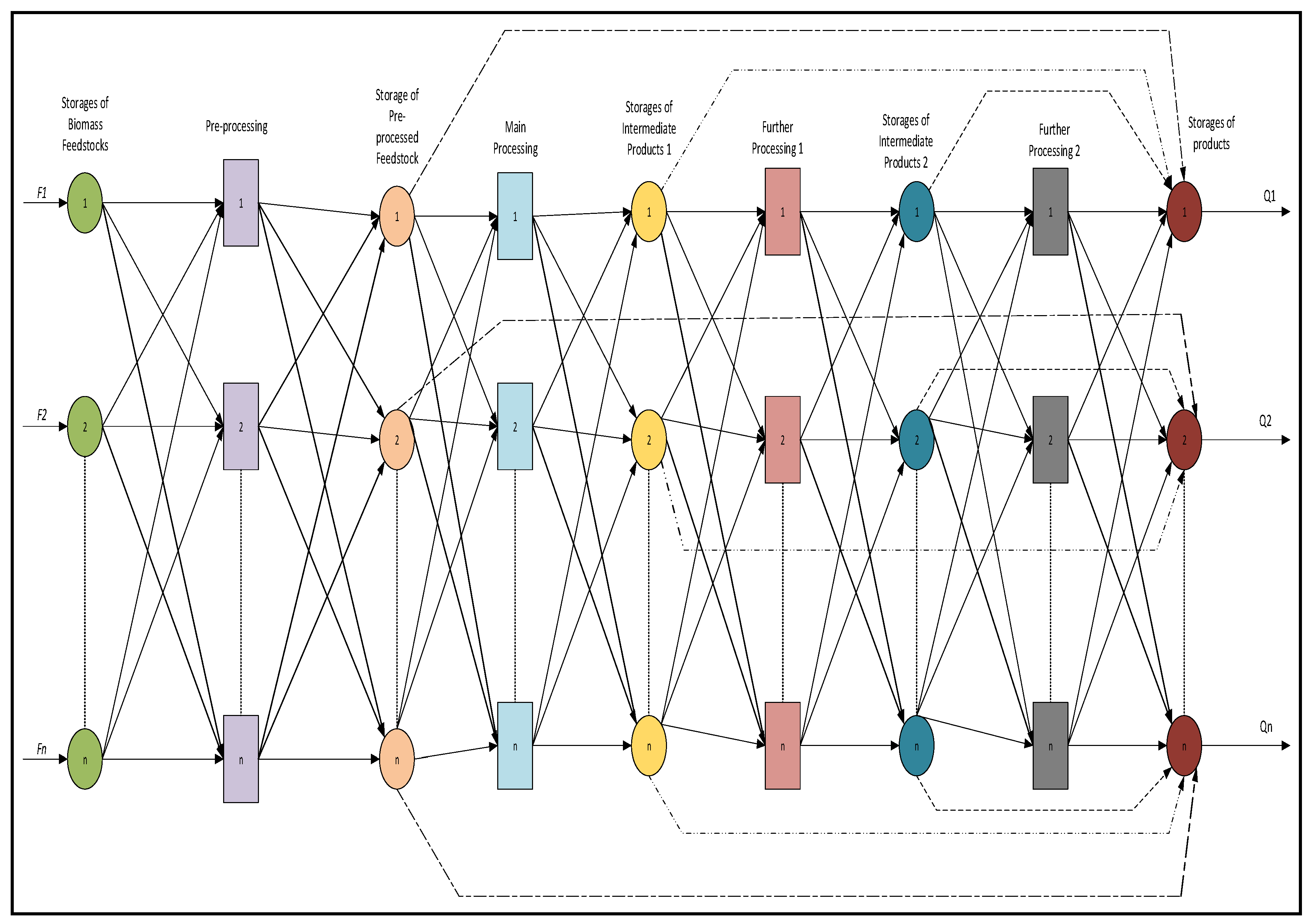
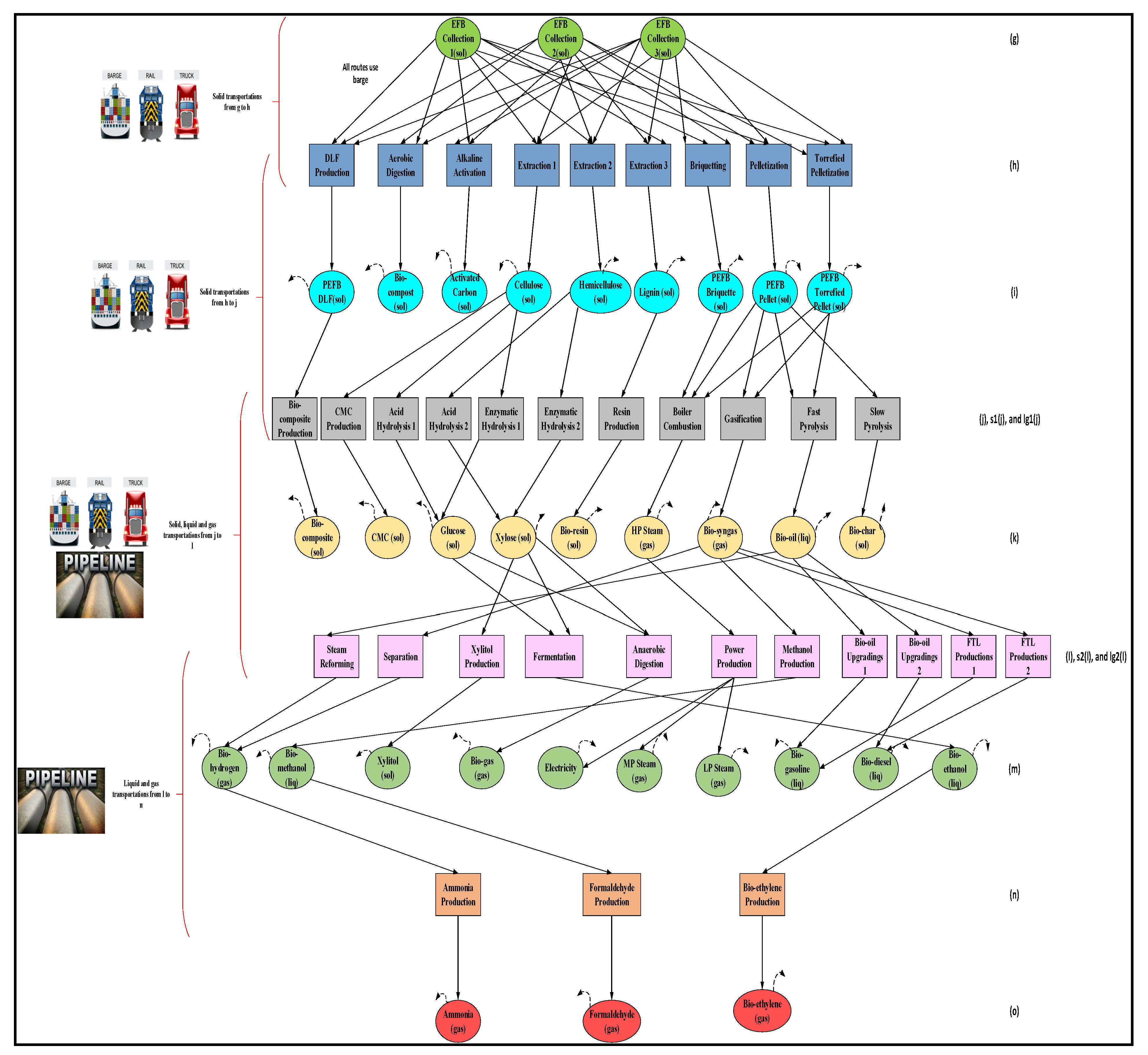
2. Materials and Methods
3. Mathematical Model for the Optimal Selections
Production cost − Emission treatment cost)
pipeline transportation operating cost
Model Parameters
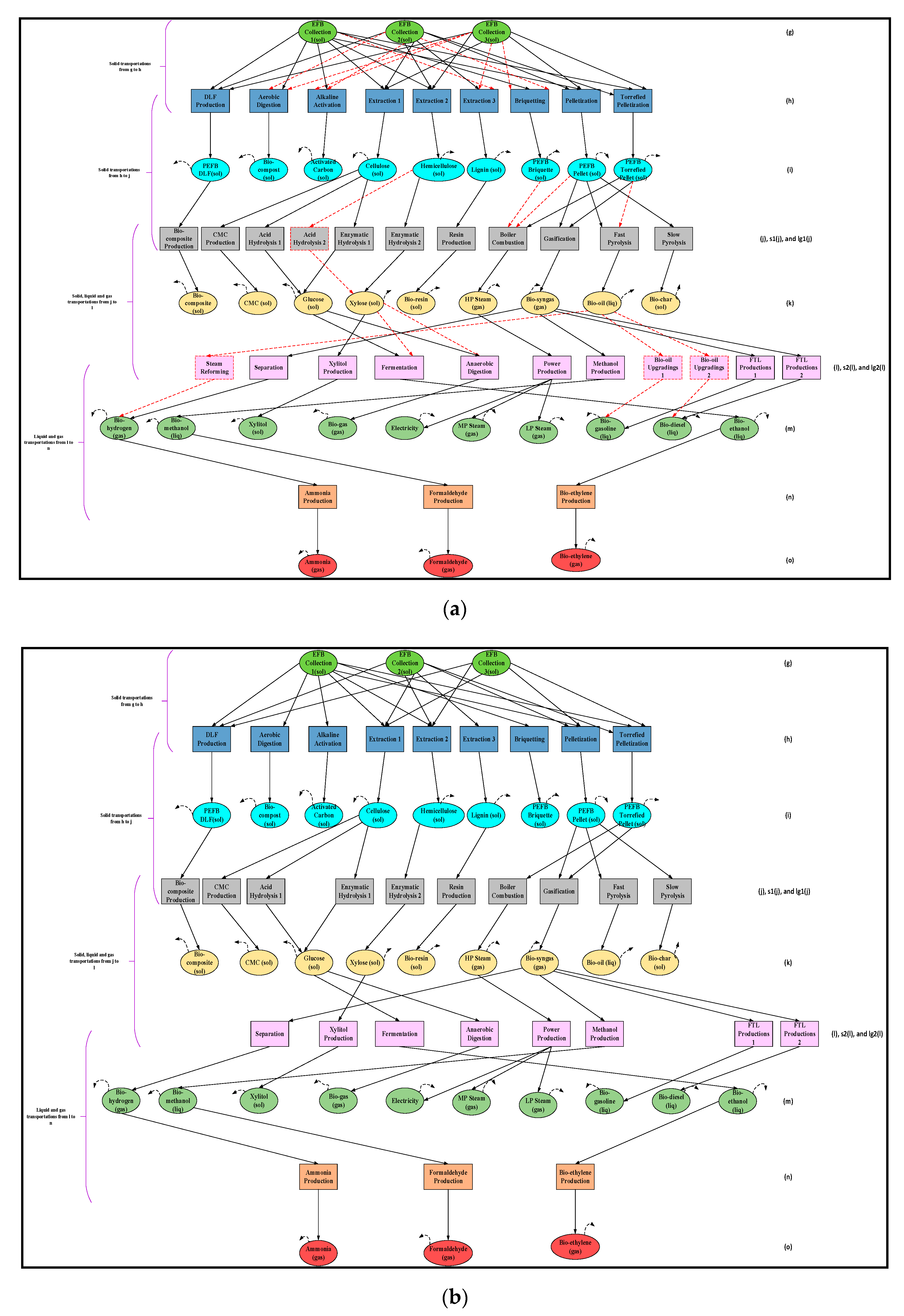
4. Results and Discussions
Sensitivity Analysis
5. Conclusions and Future Work
Author Contributions
Funding
Institutional Review Board Statement
Informed Consent Statement
Data Availability Statement
Acknowledgments
Conflicts of Interest
Appendix A

| EFB Sources Locations, g | Pre-Processing Facilities, h | Distance (km) |
|---|---|---|
| EFB Collection 1 | Aerobic Digestion On Site | 0 |
| EFB Collection 1 | DLF Production | 271 |
| EFB Collection 1 | Extraction Plant 1 | 322 |
| EFB Collection 1 | Extraction Plant 2 | 322 |
| EFB Collection 1 | Extraction Plant 3 | 322 |
| EFB Collection 1 | Briquetting Plant | 271 |
| EFB Collection 1 | Pelletization Mill | 287 |
| EFB Collection 1 | Torrefied Pelletization Mill | 208 |
| EFB Collection 1 | Alkaline Activation (Activated Carbon) Plant | 208 |
| EFB Collection 2 | Aerobic Digestion On Site | 0 |
| EFB Collection 2 | DLF Production | 165 |
| EFB Collection 2 | Extraction Plant 1 | 230 |
| EFB Collection 2 | Extraction Plant 2 | 230 |
| EFB Collection 2 | Extraction Plant 3 | 230 |
| EFB Collection 2 | Briquetting Plant | 165 |
| EFB Collection 2 | Pelletization Mill | 195 |
| EFB Collection 2 | Torrefied Pelletization Mill | 224 |
| EFB Collection 2 | Alkaline Activation (Activated Carbon) Plant | 224 |
| EFB Collection 3 | Aerobic Digestion On Site | 0 |
| EFB Collection 3 | DLF Production | 274 |
| EFB Collection 3 | Extraction Plant 1 | 486 |
| EFB Collection 3 | Extraction Plant 2 | 486 |
| EFB Collection 3 | Extraction Plant 3 | 486 |
| EFB Collection 3 | Briquetting Plant | 274 |
| EFB Collection 3 | Pelletization Mill | 289 |
| EFB Collection 3 | Torrefied Pelletization Mill | 346 |
| EFB Collection 3 | Alkaline Activation (Activated Carbon) Plant | 346 |
| Pre-Processing Facilities, h | Main Processing Facilities, j | Distance (km) |
|---|---|---|
| Extraction Plant 1 | CMC Production | 0 |
| Extraction Plant 1 | Acid Hydrolysis 1 | 546 |
| Extraction Plant 1 | Enzymatic Hydrolysis 1 | 315 |
| Extraction Plant 2 | Acid Hydrolysis 2 | 546 |
| Extraction Plant 2 | Enzymatic Hydrolysis 2 | 315 |
| Extraction Plant 3 | Resin Production | 386 |
| DLF Production | Bio-composite Production | 33 |
| Briquetting Plant | Boiler Combustion | 83 |
| Pelletization Mill | Boiler Combustion | 88 |
| Pelletization Mill | Gasification | 17 |
| Pelletization Mill | Fast Pyrolysis | 0 |
| Pelletization Mill | Slow Pyrolysis | 345 |
| Torrefied Pelletization Mill | Boiler Combustion | 23 |
| Torrefied Pelletization Mill | Gasification | 78 |
| Torrefied Pelletization Mill | Fast Pyrolysis | 86 |
| Main Processing Facilities, j | Further Processing 1 Facilities, s2(l) | Distance (km) |
|---|---|---|
| Acid Hydrolysis 2 | Xylitol Production | 0 |
| Acid Hydrolysis 1 | Anaerobic Digestion Plant | 338 |
| Enzymatic Hydrolysis 1 | Anaerobic Digestion Plant | 37 |
| Enzymatic Hydrolysis 2 | Xylitol Production | 379 |
| Main Processing Facilities, j | Further Processing 1 Facilities, lg2(l) | Distance (km) |
|---|---|---|
| Boiler Combustion | Power Production | 0 |
| Boiler Combustion | MP Steam Production | 0 |
| Boiler Combustion | LP Steam Production | 0 |
| Acid Hydrolysis (1 and 2) | Fermentation Plant (1 and 2) | 327 |
| Enzymatic Hydrolysis (1 and 2) | Fermentation Plant (1 and 2) | 65 |
| Gasification | Separation Plant | 0 |
| Gasification | Methanol Production | 404 |
| Gasification | FTL Production (1 and 2) | 19 |
| Fast Pyrolysis | Bio-oil Upgrading (1 and 2) | 94 |
| Fast Pyrolysis | Steam Reforming Plant | 0 |
| Further Processing 1 Facilities, lg2(l) | Further Processing 2 Facilities, n | Distance (km) |
|---|---|---|
| Steam Reforming Plant | Ammonia Production | 361 |
| Separation Plant | Ammonia Production | 367 |
| Methanol Production | Formaldehyde Production | 686 |
| Fermentation Plant (1 and 2) | Bio-ethylene | 316 |
| Transportation Mode | Operating Cost Factor (USD per Tonne per km) | Emission Factor (Tonnes CO2 Equivalent per Tonne per km) |
|---|---|---|
| Truck | 0.1641 | 0.000062 |
| Train | 0.0333 | 0.000022 |
| Barge | 0.0136 | 0.000015 |
| Pipeline | 0.0500 | - |
| Biomass Type, g | Pre-Processing, h | Pre-Processed Product, i | USD/Tonne | Reference |
|---|---|---|---|---|
| Blended EFBs | DLF Production | Dry Long Fiber | 85 | [26] |
| Blended EFBs | Aerobic Digestion | Bio-compost | 10 | [27] |
| Blended EFBs | Alkaline Activation | Activated Carbon | 144 | [28] |
| Blended EFBs | Extraction 1 | Cellulose | 125 | [29] |
| Blended EFBs | Extraction 2 | Hemicellulose | 130 | [29] |
| Blended EFBs | Extraction 3 | Lignin | 135 | [29] |
| Blended EFBs | Briquetting | Briquette | 50 | [30] |
| Blended EFBs | Pelletization | Pellet | 60 | [31] |
| Blended EFBs | Torrefied Pelletization | Torrefied Pellet | 70 | [31] |
| Biomass Type, g | Pre-Processing, h | Pre-Processed Product, i | Conversion Factor | Reference |
|---|---|---|---|---|
| Blended EFBs | DLF Production | Dry Long Fiber | 0.37 | [32] |
| Blended EFBs | Aerobic Digestion | Bio-compost | 0.95 | [33] |
| Blended EFBs | Alkaline Activation | Activated Carbon | 0.50 | [34] |
| Blended EFBs | Extraction 1 | Cellulose | 0.70 | Assumed value based on hemicellulose and lignin conversion factor |
| Blended EFBs | Extraction 2 | Hemicellulose | 0.15 | [35] |
| Blended EFBs | Extraction 3 | Lignin | 0.15 | [36] |
| Blended EFBs | Briquetting | Briquette | 0.38 | [32] |
| Blended EFBs | Pelletization | Pellet | 0.38 | [32] |
| Blended EFBs | Torrefied Pelletization | Torrefied Pellet | 0.38 | [32] |
| Biomass Type, g | Pre-Processing, h | Pre-Processed Product, i | CO2 Emission Factor (Tonnes CO2 Equivalent/Tonnes of Product Produced) | Reference |
|---|---|---|---|---|
| Blended EFBs | DLF Production | Dry Long Fiber | 0.0041 | [37] |
| Blended EFBs | Aerobic Digestion | Bio-compost | 0.0200 | [38] |
| Blended EFBs | Alkaline Activation | Activated Carbon | 0.0176 | [39] |
| Blended EFBs | Extraction 1 | Cellulose | 0.0590 | [29] |
| Blended EFBs | Extraction 2 | Hemicellulose | 0.0650 | [29] |
| Blended EFBs | Extraction 3 | Lignin | 0.0620 | Assumed value based on values for cellulose and hemicellulose |
| Blended EFBs | Briquetting | Briquette | 0.0500 | Assumed value |
| Blended EFBs | Pelletization | Pellet | 0.0500 | Assumed value |
| Blended EFBs | Torrefied Pelletization | Torrefied Pellet | 0.0805 | [40] |
| Pre-Processed Feedstock, i | Main Processing, j | Intermediate Product 1, k | USD/Tonne | Reference |
|---|---|---|---|---|
| Dry Long Fiber | Bio-composite Production | Bio-composite | 107.0 | [41] |
| Cellulose | CMC Production | CMC | 2500.0 | [42] |
| Cellulose | Acid Hydrolysis 1 | Glucose | 73.4 | [29] |
| Cellulose | Enzymatic Hydrolysis 1 | Glucose | 85.7 | [29] |
| Hemicellulose | Acid Hydrolysis 2 | Xylose | 168.7 | [29] |
| Hemicellulose | Enzymatic Hydrolysis 2 | Xylose | 83.1 | [29] |
| Lignin | Resin Production | Bio-resin | 1900.0 | [43] |
| Briquette | Boiler Combustion | HP Steam | 20.7 | [44] |
| Pellet | Boiler Combustion | HP Steam | 20.7 | [44] |
| Pellet | Gasification | Bio-syngas | 300.0 | Assumed value based on 50% of Bio-syngas price |
| Pellet | Fast Pyrolysis | Bio-oil | 1003 | [45] |
| Pellet | Slow Pyrolysis | Bio-char | 111.5 | [46] |
| Torrefied Pellet | Boiler Combustion | HP Steam | 20.7 | [44] |
| Torrefied Pellet | Gasification | Bio-syngas | 300.0 | Assumed value based on 50% of Bio-syngas price |
| Torrefied Pellet | Fast Pyrolysis | Bio-oil | 1003 | [45] |
| Pre-Processed Feedstock, i | Main Processing, j | Intermediate Product 1, k | Conversion Factor | Reference |
|---|---|---|---|---|
| Dry Long Fiber | Bio-composite Production | Bio-composite | 0.75 | [47] |
| Cellulose | CMC Production | CMC | 0.86 | [48] |
| Cellulose | Acid Hydrolysis 1 | Glucose | 0.37 | [29] |
| Cellulose | Enzymatic Hydrolysis 1 | Glucose | 0.47 | [29] |
| Hemicellulose | Acid Hydrolysis 2 | Xylose | 0.91 | [28] |
| Hemicellulose | Enzymatic Hydrolysis 2 | Xylose | 0.88 | [29] |
| Lignin | Resin Production | Bio-resin | 0.95 | [49] |
| Briquette | Boiler Combustion | HP Steam | 0.20 | [50] |
| Pellet | Boiler Combustion | HP Steam | 0.25 | [50] |
| Pellet | Gasification | Bio-syngas | 0.70 | [51] |
| Pellet | Fast Pyrolysis | Bio-oil | 0.60 | [52] |
| Pellet | Slow Pyrolysis | Bio-char | 0.50 | [53] |
| Torrefied Pellet | Boiler Combustion | HP Steam | 0.30 | [50] |
| Torrefied Pellet | Gasification | Bio-syngas | 0.80 | [51] |
| Torrefied Pellet | Fast Pyrolysis | Bio-oil | 0.60 | [54] |
| Pre-Processed Feedstock, i | Main Processing, j | Intermediate Product 1, k | CO2 Emission Factor (Tonnes CO2 Equivalent/Tonnes of Product Produced) | Reference |
|---|---|---|---|---|
| Dry Long Fiber | Bio-composite Production | Bio-composite | 7.481 | [55] |
| Cellulose | CMC Production | CMC | 0.097 | Assumed value |
| Cellulose | Acid Hydrolysis 1 | Glucose | 0.097 | [29] |
| Cellulose | Enzymatic Hydrolysis 1 | Glucose | 0.085 | [29] |
| Hemicellulose | Acid Hydrolysis 2 | Xylose | 0.075 | [29] |
| Hemicellulose | Enzymatic Hydrolysis 2 | Xylose | 0.082 | [29] |
| Lignin | Resin Production | Bio-resin | 2.500 | [56] |
| Briquette | Boiler Combustion | HP Steam | 0.750 | [57] |
| Pellet | Boiler Combustion | HP Steam | 0.750 | Assumed value |
| Pellet | Gasification | Bio-syngas | 0.680 | [58] |
| Pellet | Fast Pyrolysis | Bio-oil | 0.580 | [52] |
| Pellet | Slow Pyrolysis | Bio-char | 0.580 | [52] |
| Torrefied Pellet | Boiler Combustion | HP Steam | 0.750 | Assumed value |
| Torrefied Pellet | Gasification | Bio-syngas | 0.680 | [58] |
| Torrefied Pellet | Fast Pyrolysis | Bio-oil | 0.580 | [52] |
| Intermediate Product 1, k | Further Processing 1, s2(l) | Intermediate Product 2, m | USD/Tonne | Reference |
|---|---|---|---|---|
| Glucose | Anaerobic Digestion | Bio-gas | 199.0 | Assumed value for 50% less of the bio-gas price |
| Xylose | Anaerobic Digestion | Bio-gas | 199.0 | Assumed value for 50% less of the bio-gas price |
| Xylose | Xylitol Production | Xylitol | 2100.0 | Assumed value for 50% less of the xylitol price |
| Intermediate Product 1, k | Further Processing 1, lg2(l) | Intermediate Product 2, m | USD/Tonne or MWh | Reference |
|---|---|---|---|---|
| Bio-oil | Steam Reforming | Bio-hydrogen | 455.0 | [59] |
| Bio-oil | Bio-oil Upgrading 1 | Bio-gasoline | 1089.0 | [60] |
| Bio-oil | Bio-oil Upgrading 2 | Bio-diesel | 918.0 | [60] |
| Glucose | Fermentation 1 | Bio-ethanol | 98.2 | [29] |
| Xylose | Fermentation 2 | Bio-ethanol | 98.2 | [29] |
| HP Steam | Power Production | Electricity | 58.9/MWh | [50] |
| HP Steam | Power Production | MP Steam | 12.0 | Assumed valued based on the steam price |
| HP Steam | Power Production | LP Steam | 7.0 | Assumed valued based on the steam price |
| Bio-syngas | Methanol Production | Bio-methanol | 83.6 | [29] |
| Bio-syngas | Separation | Bio-hydrogen | 112 | [61] |
| Bio-syngas | FTL Productions 2 | Bio-diesel | 167.3 | [29] |
| Bio-syngas | FTL Productions 1 | Bio-gasoline | 519.8 | [60] |
| Intermediate Product 1, k | Further Processing 1, s2(l) | Intermediate Product 2, m | Conversion Factor | Reference |
|---|---|---|---|---|
| Glucose | Anaerobic Digestion | Bio-gas | 0.70 | [33] |
| Xylose | Anaerobic Digestion | Bio-gas | 0.70 | [33] |
| Xylose | Xylitol Production | Xylitol | 0.70 | [62] |
| Intermediate Product 1, k | Further Processing 1, lg2(l) | Intermediate Product 2, m | Conversion Factor | Reference |
|---|---|---|---|---|
| Bio-oil | Steam Reforming | Bio-hydrogen | 0.84 | [63] |
| Bio-oil | Bio-oil Upgrading 1 | Bio-gasoline | 0.40 | [64] |
| Bio-oil | Bio-oil Upgrading 2 | Bio-diesel | 0.20 | [64] |
| Glucose | Fermentation 1 | Bio-ethanol | 0.33 | [29] |
| Xylose | Fermentation 2 | Bio-ethanol | 0.33 | [29] |
| HP Steam | Power Production | Electricity | 0.30 MWh/tonne of steam | [65] |
| HP Steam | Power Production | MP Steam | 0.35 | [32] |
| HP Steam | Power Production | LP Steam | 0.35 | [32] |
| Bio-syngas | Methanol Production | Bio-methanol | 0.41 | [29] |
| Bio-syngas | Separation | Bio-hydrogen | 0.46 | [29] |
| Bio-syngas | FTL Productions 2 | Bio-diesel | 0.71 | [51] |
| Bio-syngas | FTL Productions 1 | Bio-gasoline | 0.29 | Assumed value from bio-diesel conversion factor |
| Intermediate Product 1, k | Further Processing 1, s2(l) | Intermediate Product 2, m | CO2 Emission Factor (Tonnes CO2 Equivalent/Tonnes of Product Produced) | Reference |
|---|---|---|---|---|
| Glucose | Anaerobic Digestion | Bio-gas | 0.250 | [66] |
| Xylose | Anaerobic Digestion | Bio-gas | 0.250 | [66] |
| Xylose | Xylitol Production | Xylitol | 0.082 | Assumed value based on value of xylose |
| Intermediate Product 1, k | Further Processing 1, lg2(l) | Intermediate Product 2, m | CO2 Emission Factor (Tonnes CO2 Equivalent/Tonnes of Product Produced) | Reference |
|---|---|---|---|---|
| Bio-oil | Steam Reforming | Bio-hydrogen | 16.930 | [52] |
| Bio-oil | Bio-oil Upgrading 1 | Bio-gasoline | 13.000 | [52] |
| Bio-oil | Bio-oil Upgrading 2 | Bio-diesel | 13.000 | [52] |
| Glucose | Fermentation 1 | Bio-ethanol | 0.098 | [29] |
| Xylose | Fermentation 2 | Bio-ethanol | 0.098 | [29] |
| HP Steam | Power Production | Electricity | 0.050 | Assumed value |
| HP Steam | Power Production | MP Steam | 0.050 | Assumed value |
| HP Steam | Power Production | LP Steam | 0.050 | Assumed value |
| Bio-syngas | Methanol Production | Bio-methanol | 0.083 | [29] |
| Bio-syngas | Separation | Bio-hydrogen | 0.090 | [29] |
| Bio-syngas | FTL Productions 2 | Bio-diesel | 0.067 | [29] |
| Bio-syngas | FTL Productions 1 | Bio-gasoline | 0.639 | [29] |
| Intermediate Product 2, m | Further Processing 2, n | Final Product, p | USD/Tonne | Reference |
|---|---|---|---|---|
| Bio-hydrogen | Ammonia Production | Ammonia | 377 | [67] |
| Bio-methanol | Formaldehyde Production | Formaldehyde | 232 | [68] |
| Bio-ethanol | Bio-ethylene Production | Bio-ethylene | 1200 | [46] |
| Intermediate Product 2, m | Further Processing 2, n | Final Product, p | Conversion Factor | Reference |
|---|---|---|---|---|
| Bio-hydrogen | Ammonia Production | Ammonia | 0.80 | [67] |
| Bio-methanol | Formaldehyde Production | Formaldehyde | 0.97 | [69] |
| Bio-ethanol | Bio-ethylene Production | Bio-ethylene | 0.99 | [46] |
| Intermediate Product 2, m | Further Processing 2, n | Final Product, p | CO2 Emission Factor (Tonnes CO2 Equivalent/Tonnes of Product Produced) | Reference |
|---|---|---|---|---|
| Bio-hydrogen | Ammonia Production | Ammonia | 1.694 | [70] |
| Bio-methanol | Formaldehyde Production | Formaldehyde | 0.083 | Assumed value |
| Bio-ethanol | Bio-ethylene Production | Bio-ethylene | 1.400 | [46] |
References
- Alang Mahat, S. The Palm Oil Industry from the Perspective of Sustainable Development: A Case Study of Malaysian Palm Oil Industry. Master’s Thesis, Ritsumeikan Asia Pacific University, Beppu, Japan, 2012. [Google Scholar]
- May, C.Y. Malaysian Palm Oil Industry-Enhancing Competitiveness in Meeting Challenges; Presentation Slides for Malaysia-Romania Palm Oil Trade Fair and Seminar; Malaysia-Romania Palm Oil Trade Fair and Seminar (POTS): Bucharest, Romania, 2011. [Google Scholar]
- Sustainable Palm Oil Development in Malaysia. Available online: https://www.palmoilworld.org/sustainability.html (accessed on 24 February 2015).
- Simeh, A.; Tengku Ahmad, T.M.A. The Case Study on Malaysian Palm Oil. In Proceedings of the Regional Workshop on Commodity Export Diversification and Poverty Reduction in South and South-East Asia, Bangkok, Thailand, 3–5 April 2001. [Google Scholar]
- Zailan, R.; Lim, J.S.; Manan, Z.A.; Alwi, S.R.; Mohammadi-ivatloo, B.; Jamaluddin, K. Malaysia scenario of biomass supply chain-cogeneration system and optimization modeling development: A review. Renew. Sustain. Energy Rev. 2021, 148, 111289. [Google Scholar] [CrossRef]
- Nagel, J. Determination of an Economic Energy Supply Structure Based on Biomass Using a Mixed-Integer Linear Optimization Model. Ecol. Eng. 2000, 16, S91–S102. [Google Scholar] [CrossRef]
- Gelson, T.; Epplin Francis, M.; Huhnke Raymond, L. Integrative Investment Appraisal of a Lignocellulosic Biomass-to-Ethanol Industry. J. Agric. Resour. Econ. 2003, 28, 611–633. [Google Scholar]
- Huang, Y.; Chen, C.W.; Fan, Y. Multistage Optimization of the Supply Chains of Biofuels. Transp. Res. Part E Logist. Transp. Rev. 2010, 46, 820–830. [Google Scholar] [CrossRef]
- Marvin, W.A.; Schmidt, L.D.; Benjaafar, S.; Tiffany, D.G.; Daoutidis, P. Economic Optimization of a Lignocellulosic Biomass-to-Ethanol Supply Chain. Chem. Eng. Sci. 2011, 67, 68–79. [Google Scholar] [CrossRef]
- You, F.; Wang, B. Life Cycle Optimization of Biomass-to-Liquid Supply Chains with Distributed-Centralized Processing Networks. Ind. Eng. Chem. Res. 2011, 50, 10102–10127. [Google Scholar] [CrossRef]
- Bowling, I.M.; Ponce-Ortega, J.M.; El-Halwagi, M.M. Facility Location and Supply Chain Optimization for a Biorefinery. Ind. Eng. Chem. Res. 2011, 50, 6276–6286. [Google Scholar] [CrossRef]
- Zhang, L. and Hu, G. Supply Chain Design and Operational Planning Models for Biomass to Drop-in Biofuel Production. Biomass Bioenergy 2013, 58, 238–250. [Google Scholar] [CrossRef] [Green Version]
- Lin, T.; Rodriguez, L.F.; Shastri, Y.N.; Hansen, A.C.; Ting, K.C. Integrated Strategic and Tactical Biomass-Biofuel Supply Chain Optimization. Bioresour. Technol. 2014, 156, 256–266. [Google Scholar] [CrossRef]
- Paulo, H.; Azcue, X.; Barbosa-Povoa, A.P.; Relvas, S. Supply Chain Optimization of Residual Forestry Biomass for Bioenergy Production: The Case Study of Portugal. Biomass Bioenergy 2015, 83, 245–256. [Google Scholar] [CrossRef]
- Razik, A.H.A.; Khor, C.S.; Elkamel, A. A model-based approach for biomass-to-bioproducts supply Chain network planning optimization. Food Bioprod. Process. 2019, 118, 293–305. [Google Scholar] [CrossRef]
- Tapia, J.F.; Samsatli, S. Integrating fuzzy analytic hierarchy process into a multi- objective optimisation model for planning sustainable oil palm value chains. Food Bioprod. Process. 2020, 119, 48–74. [Google Scholar] [CrossRef]
- Zailan, R.; Lim, J.S.; Sa’ad, S.F.; Jamaluddin, K.; Abdulrazik, A. Optimal Biomass Cogeneration Facilities Considering Operation and Maintenance. Chem. Eng. Trans. 2021, 89, 517–522. [Google Scholar]
- Guo, C.; Hu, H.; Wang, S.; Rodriguez, L.F.; Ting, K.C.; Lin, T. Multiperiod stochastic programming for biomass supply chain design under spatiotemporal variability of feedstock supply. Renew. Energy 2022, 186, 378–393. [Google Scholar] [CrossRef]
- Asghari, M.; Fathollahi-Fard, A.M.; Mirzapour Al-e-hashem, S.M.J.; Dulebenets, M.A. Transformation and Linearization Techniques in Optimization: A State-of-the-Art Survey. Mathematics 2022, 10, 283. [Google Scholar] [CrossRef]
- Albayrak, I.; Sivri, M.; Temelcan, G. A New Successive Linearization Approach for Solving Nonlinear Programming Problems. Appl. Appl. Math. Int. J. 2019, 14, 30. [Google Scholar]
- Abdulrazik, A.; Elsholkami, M.; Elkamel, A.; Simon, L. Multi-products Productions from Malaysian Oil Palm Empty Fruit Bunch (EFB): Analyzing Economic Potentials from the Optimized Biomass Supply Chains. J. Clean. Prod. 2017, 168, 131–148. [Google Scholar] [CrossRef] [Green Version]
- Oo, A.; Kelly, J.; Lalonde, C. Assessment of Business Case for Purpose-Grown Biomass in Ontario; A Report for Ontario Federation of Agriculture; The Western University Research Park: Ontario, ON, Canada, 2012. [Google Scholar]
- Grossmann, I.E.; Trespalacios, F. Review of Mixed Integer Nonlinear and Generalized Disjunctive Programming Methods in Process System Engineering. Chem. Ing. Tech. 2014, 86, 991–1012. [Google Scholar]
- Grossmann, I.E. Mixed Integer Nonlinear Programming for Process System Engineering; Department of Chemical Engineering, Carnegie Mellon University: Pittsburgh, PA, USA, 1999. [Google Scholar]
- Mckinnon, A. CO2 Emission from Freight Transport: An Analysis of UK Data; Logistic Research Centre, Heriot-Watt University: Edinburgh, UK, 2008. [Google Scholar]
- Production Cost for Fiber. Available online: https://www.hempfarm.org/Papers/Market_Analysis_for_Hemp.html (accessed on 16 July 2014).
- Fabian, E.E.; Richard, T.L.; Kay, D. A Report of Agricultural Composting: A Feasibility Study for New York Farms; Cornell Waste Management Institute, Cornell University: New York, NY, USA, 1993. [Google Scholar]
- Lima, I.M.; McAloon, A.; Baoteng, A.A. Activated Carbon from Broiler Litter: Process Description and Cost of Production. Biomass Bioenergy 2008, 32, 568–572. [Google Scholar] [CrossRef]
- Murillo-Alvarado, P.E.; Ponce-Ortega, J.M.; Serna-Gonzalez, M.; Castro-Montoya, A.J.; El-Halwagi, M.M. Optimization of Pathways for Biorefineries Involving the Selection of Feedstocks, Products, and Processing Steps. Ind. Eng. Chem. Res. 2013, 52, 5177–5190. [Google Scholar] [CrossRef]
- Kanna, S.U. Value Addition of Agroforestry Residues through Briquetting Technology for Energy Purpose; Presentation Slides, Forest College and Research Institute, Tamil Nadu Agricultural University: Tamil Nadu, India, 2010. [Google Scholar]
- Ontario Federation of Agriculture. Literature Review and Study Energy Market Alternatives for Commercially Grown Biomass in Ontario; A Report for Ontario Federation of Agriculture; PPD Technologies Inc.: Ontario, ON, Canada, 2011. [Google Scholar]
- Ng, R.T.L.; Denny Ng, D.K.S. Systematic Approach for Synthesis of Integrated Palm Oil Processing Complex. Part 1: Single Owner. Ind. Chem. Res. 2013, 52, 102061–102220. [Google Scholar] [CrossRef]
- Hubbe, M.A.; Nazhad, M.; Sanchez, C. Composting as a Way to Convert Cellulosic Biomass and Organic Waste into High-Value Soil Amendments: A Review. BioResources 2010, 5, 2808–2854. [Google Scholar] [CrossRef]
- Kaghazchi, T.; Soleimani, M.; Yeganeh, M.M. Production of Activated Carbon from Residue of Liquorices Chemical Activation. In Proceedings of the 8th Asia-Pacific International Symposium on Combustion and Energy Utilization, Sochi, Russia, 10–12, October 2006; ISBN 5-89238-086-6. [Google Scholar]
- Hemicellulose Extraction Efficiency. Available online: https://ipst.gatech.edu/faculty/ragauskas_art/research_opps/Hemicellulose%20Extraction%20for%20Enhanced%20Biofuels%20Production.pdf (accessed on 16 July 2014).
- Lignin Production Efficiency. Available online: https://purelignin.com/products (accessed on 16 July 2014).
- Carbon Dioxide Emission Factor for DLF. Available online: https://oecotextiles.wordpress.com/2011/01/19/estimating-the-carbon-footprint-of-a-fabric/ (accessed on 4 August 2014).
- Composting CO2 Emission Factor. Available online: epa.gov/epawaste/conserve/tools/warm/pdfs/Composting_Overview.pdf (accessed on 22 November 2014).
- Carbon Dioxide Emission Factor for Activated Carbon. Available online: www.omnipure.com/sustain/emissions.htm (accessed on 22 November 2014).
- Kaliyan, N.; Morey, R.V.; Tiffany, D.G.; Lee, W.F. Life Cycle Assessment of Corn Stover Torrefaction Plant Integrated with Corn Ethanol Plant and Coal Fired Power Plant. Biomass Bioenergy 2014, 63, 92–100. [Google Scholar] [CrossRef]
- Economic Research Institute for ASEAN and East Asian. Price and Production Cost of Bio-composites from Oil Palm. Available online: www.eria.org (accessed on 22 November 2014).
- Carboxy Methyl Cellulose (CMC) Selling Price and Production Cost Estimation. Available online: https://trade.ec.europa.eu/doclib/html/112178.htm (accessed on 9 July 2014).
- Chiarakorn, S.; Permpoonwiwat, C.K.; Nanthachatchavankul, P. Cost Benefit Analysis of Bioplastic Production in Thailand. Econ. Public Policy J. 2012, 3, 44–73. [Google Scholar]
- Steam Production Cost from Energy Efficiency & Renewable Energy. Available online: https://www1.eere.energy.gov/manufacturing/tech_assistance/pdfs/steam15_benchmark.pdf (accessed on 19 July 2014).
- Thorp, B.A. Key Metric Comparison of Five Cellulosic Biofuel Pathways, Advances. In Developments, Applications in the Field of Cellulosic Biomass; TAPPI: Atlanta, GA, USA, 2010. [Google Scholar]
- Production of Bio-ethylene. Available online: https://irena.org/-/media/Files/IRENA/Agency/Publication/2013/IRENA-ETSAP-Tech-Brief-I13-Production_of_Bio-ethylene.pdf (accessed on 24 November 2014).
- Karbstein, H.; Funk, J.; Norton, J.; Nordmann, G. Lightweight Bio-Composites with Acrodur resin Technology; Presentation Slides; BASF AG: Beaumont, TX, USA, 2013. [Google Scholar]
- Saputra, A.H.; Qadhayna, L.; Pitaloka, A.B. Synthesis and Characterization of CMC from Water Hyacinth using Ethanol-Isobutyl Alcohol Mixture as Solvents. Int. J. Chem. Eng. Appl. 2014, 5, 36–40. [Google Scholar] [CrossRef] [Green Version]
- Yin, Q.; Yang, W.; Sun, C.; Di, M. Preparation and Properties of Lignin-Epoxy Resin Composite. Bioresources 2012, 7, 5737–5748. [Google Scholar] [CrossRef] [Green Version]
- Searcy, E.; Flynn, P. The Impact of Biomass Availability and Processing Cost on Optimum Size and Processing Technology Selection. Appl. Biochem. Biotechnol. 2009, 154, 271–286. [Google Scholar] [CrossRef]
- Boerrigter, H.; van der Drift, B. Biosyngas Key-Intermediate in Production of Renewable Transportation Fuels, Chemicals, and Electricity: Optimum Scale and Economic Prospects of Fischer-Tropsch Plants. In Proceedings of the 14th European Biomass Conference & Exhibition, Paris, France, 17–21 October 2005. [Google Scholar]
- Zhang, Y.; Brown, T.R.; Hu, G.; Brown, R.C. Techno-economic Analysis of Two Bio-Oil Upgrading Pathways. Chem. Eng. J. 2013, 225, 895–904. [Google Scholar] [CrossRef]
- Conversion Factor of Bio-Char Production. Available online: https://biocharfarms.org/biochar_production_energy/ (accessed on 23 July 2014).
- Zhang, Y.; Hu, G.; Brown, R.C. Life Cycle Assessment of the Production of Hydrogen and Transportation Fuels from Corn Stover via Fast Pyrolysis. Environ. Res. Lett. 2013, 8, 025001. [Google Scholar] [CrossRef] [Green Version]
- Carbon Dioxide Emission Factor for Bio-Composite Production. Available online: winrigo.com.sg/pdf/WinrigoCatalogue.pdf (accessed on 25 November 2014).
- Carbon Dioxide Emission Factor for Bio-Resin Production. Available online: https://www.netcomposites.com/news/sustainable-industrial-resins-from-vegetable-oil/4239 (accessed on 25 November 2014).
- Carbon Dioxide Emission Factor for Briquette Utilization. Available online: https://www.sarawakenergy.com.my/index.php/r-d/biomass-energy/palm-oil-biomass (accessed on 25 November 2014).
- Basu, P. Biomass Gasification, Pyrolysis and Torrefaction: Practical Design and Theory, 2nd ed.; Academic Press: London, UK, 2013. [Google Scholar]
- Sarkar, S.; Kumar, A. Large-scale Bio-hydrogen Production from Bio-oil. Bioresour. Technol. 2010, 101, 7350–7361. [Google Scholar] [CrossRef]
- Wright, M.M.; Brown, R.C. Costs of Thermochemical Conversion of Biomass to Power and Liquid Fuels (Chapter 10). In Thermochemical Processing of Biomass Conversion into Fuels, Chemicals and Power; John Wiley & Sons, Ltd.: Hoboken, NJ, USA, 2011. [Google Scholar]
- Schubert, P.J. Bio-Hydrogen for Power Plants; Presentation Slides for TransTech Energy Conference; West Virginia University: Morgantown, WV, USA, 2013. [Google Scholar]
- Prakasham, R.S.; Rao, S.; Hobbs, P.J. Current Trends in Biotechnological Production of Xylitol and Future Prospects. Curr. Trends Biotechnol. Pharm. 2009, 3, 8–36. [Google Scholar]
- Dillich, S. Distributed Bio-Oil Reforming; A Report for the National Renewable Energy Laboratory (NREL); Office of Energy Efficiency & Renewable Energy: Washington, DC, USA, 2013.
- Kim, J.; Realff, M.J.; Lee, J.H. Optimal Design and Global Sensitivity Analysis of Biomass Supply Chain Networks for Biofuels under Uncertainty. Comput. Chem. Eng. 2011, 35, 1738–1751. [Google Scholar] [CrossRef]
- Steam Turbine Efficiency. Available online: https://www.turbinesinfo.com/steam-turbine-efficiency (accessed on 21 July 2014).
- Whiting, A.; Azapagic, A. Life Cycle Environmental Impacts of Generating Electricity and Heat from Biogas Produced from Anaerobic Digestion. Energy 2014, 70, 181–193. [Google Scholar] [CrossRef]
- Conversion Factor and Cost for Ammonia Production. Available online: https://www.hydrogen.energy.gov/pdfs/nh3_paper.pdf (accessed on 21 July 2014).
- Chemicals Prices and Demands. Available online: http://www.icis.com/contact/free-sample-price-report (accessed on 13 May 2014).
- Chu, P.M.; Thorn, W.J.; Sams, R.L.; Guenther, F.R. On-Demand Generation of a Formaldehyde-in-Air Standard. J. Res. Natl. Inst. Stand. Technol. 1997, 102, 559–568. [Google Scholar] [CrossRef] [PubMed]
- Jubb, C.; Nakhutin, A.; Cianci, V.C.S. Chapter 3: Chemical Industry Emissions. In 2006 IPCC Guidelines for National Greenhouse Gas Inventories; Institute for Global Environmental Strategies (IGES): Hayama, Japan, 2006. [Google Scholar]

| Indices | Description | Contents |
|---|---|---|
| g | Biomass source storage locations | EFB1, EFB2, and EFB3. |
| h | Pre-processing facilities | DLF production, aerobic digestion, alkaline activation, extraction 1, extraction 2, extraction 3, briquetting, pelletization, and torrefied pelletization. |
| j | Main processing facilities | Bio-composite production, CMC production, acid hydrolysis 1, acid hydrolysis 2, enzymatic hydrolysis 1, enzymatic hydrolysis 2, resin production, boiler combustion, gasification, fast pyrolysis, and slow pyrolysis. |
| l | Further processing 1 facilities | Steam reforming, separation, xylitol production, fermentation, anaerobic digestion, power production, methanol production, bio-oil upgrading 1, bio-oil upgrading 2, FTL production 1, and FTL production 2. |
| n | Further processing 2 facilities | Ammonia production, formaldehyde production, and bio-ethylene production. |
| p | Product sum up type p storages and to the users | PEFB-DLF, bio-compost, activated carbon, cellulose, hemicellulose, lignin, PFB briquette, PEFB pellet, PEFB torrefied pellet, bio-composite, CMC, glucose, xylose, bio-resin, HP steam, bio-syngas, bio-oil, bio-char, bio-hydrogen, xylitol, bio-ethanol, bio-gas, bio-methanol, electricity, MP steam, LP steam, bio-ethylene, bio-diesel, bio-gasoline, ammonia, and formaldehyde. |
| Further aspects of the indices and descriptions for the model’s formulation | ||
| i(p) | Pre-processed feedstocks storages | PEFB-DLF, bio-compost, activated carbon, cellulose, hemicellulose, lignin, PFB briquette, PEFB pellet, and PEFB torrefied pellet. |
| k(p) | Intermediate products 1 storages | Bio-composite, CMC, glucose, xylose, bio-resin, HP steam, bio-syngas, bio-oil, and bio-char. |
| lg2(l) | Further processing 1 facilities for solid solution and liquid and gaseous feeds | Steam reforming, separation, power production, MP steam production, LP steam production, methanol production, bio-oil upgrading 1, bio-oil upgrading 2, FTL production 1, FTL production 2, and fermentation. |
| lg1(j) | Main processing facilities for liquid and gaseous products to the next processing facilities | Boiler combustion, gasification, and fast pyrolysis. |
| m(p) | Intermediate products 2 storages | Bio-hydrogen, xylitol, bio-ethanol, bio-gas, bio-methanol, electricity, MP steam, LP steam, bio-diesel, and bio-gasoline. |
| o(p) | Final products storages | Ammonia, formaldehyde, and bio-ethylene. |
| s1(j) | Main processing facilities for solid products to the next processing facilities | Acid hydrolysis 1, acid hydrolysis 2, enzymatic hydrolysis 1, and enzymatic hydrolysis 2. |
| s2(l) | Further processing 1 facilities for solid feeds | Xylitol production and anaerobic digestion. |
| t | Truck, train, and barge transportation | Truck, train, and barge. |
| z | Pipeline transportation | Pipeline. |
| Formulation | Description |
|---|---|
| 1 | Objective function |
| 2 | Equation to calculate total sales of products in USD per year |
| 3 | Equation to calculate total EFB costs in USD per year |
| 4 | Components in transportation operating costs |
| 5 | Equation to calculate transportation operating costs for truck, train, and barge in USD per year |
| 6 | Equation to calculate transportation operating costs for pipeline in USD per year |
| 7 | Total amount of biomass transported from g to h using transportation t in tonnes per year |
| 8 | Total amount of pre-processed products transported from h to j using transportation t in tonnes per year |
| 9 | Total amount of solid intermediate products 1 transported from s1(j) to s2(l) using transportation t in tonnes per year |
| 10 | Total amount of liquid and gaseous intermediate products 1 transported from lg1(j) to lg2(l) using transportation z in tonnes per year |
| 11 | Total amount of intermediate products 2 transported from lg2(l) to n using transportation z in tonnes per year |
| 12 | Equation to calculate production cost in USD per year |
| 13 | Components in emission treatment costs |
| 14 | Equation to calculate emission treatment costs from productions in USD per year |
| 15 | Equation to calculate emission treatment costs from transportations in USD per year |
| 16 | Equation to calculate emission at h to produce i in tonnes CO2 equivalent per year |
| 17 | Equation to calculate emission at j to produce k in tonnes CO2 equivalent per year |
| 18 | Equation to calculate emission at s2(l) to produce m in tonnes CO2 equivalent per year |
| 19 | Equation to calculate emission at lg2(l) to produce m in tonnes CO2 equivalent per year |
| 20 | Equation to calculate emission at n to produce o in tonnes CO2 equivalent per year |
| 21 | Equation to calculate emission from transportation between g and h using transportation mode t in tonnes CO2 equivalent per year |
| 22 | Equation to calculate emission from transportation between h and j using transportation mode t in tonnes CO2 equivalent per year |
| 23 | Equation to calculate emission from transportation between j and s2(l) using transportation mode t in tonnes CO2 equivalent per year |
| 24 | Amount of EFB in tonnes per year must not exceed the availability |
| 25 | Range of amounts of produced products in tonnes or MWh per year |
| 26 | Mass balance for EFB sources’ storage outlets in tonnes per year |
| 27 | Mass balance for yield of pre-processed feedstocks in tonnes per year |
| 28 | Mass balance for pre-processing facilities outlets in tonnes per year |
| 29 | Mass balance for yield of intermediate products 1 in tonnes per year |
| 30 | Mass balance for main processing facilities outlets in tonnes per year |
| 31 | Mass balance for yield of intermediate products 2 from solid feeds in tonnes per year |
| 32 | Mass balance for yield of intermediate products 2 from solid solution and liquid and gaseous feeds in tonnes per year |
| 33 | Mass balance of s2(l) in tonnes per year |
| 34 | Mass balance of lg2(l) in tonnes per year |
| 35 | Mass balance for yield of final products in tonnes per year |
| 36 | Mass balance for further processing facilities 2 outlets in tonnes per year |
| 37 | Summation of products at i in tonnes per year |
| 38 | Summation of products at k in tonnes per year |
| 39 | Summation of products at m in tonnes per year |
| 40 | Summation of products at o in tonnes per year |
| 41 | Maximum capacity for transportation t from g to h in tonnes per year |
| 42 | Maximum capacity for transportation t from h to j in tonnes per year |
| 43 | Maximum capacity for transportation t for solid from j to l in tonnes per year |
| 44 | Maximum capacity for transportation z for liquid and gas from j to l in tonnes per year |
| 45 | Maximum capacity for transportation z for liquid and gas from l to n in tonnes per year |
| 46 | Integer decision for mode of transportation from g to h |
| 47 | Integer decision for mode of transportation from h to j |
| 48 | Integer decision for mode of transportation from s1(j) to s2(l) |
| 49 | Integer decision for mode of transportation from lg1(j) to lg2(l) |
| 50 | Integer decision for mode of transportation from lg2(l) to n |
| 51 | Integer decision for best processing route at h to produce i |
| 52 | Integer decision for best processing route at j to produce k |
| 53 | Integer decision for best processing route at s2(l) to produce m |
| 54 | Integer decision for best processing route at lg2(l) to produce m |
| 55 | Summation for transporting solid fraction X using transportation t |
| 56 | Summation for transporting liquid and gas fractions ZZ using transportation z |
| 57 | Upper and lower limits of capacity for transportation t at each processing route |
| 58 | Upper and lower limits of capacity for transportation z at each processing route |
| Term | Category | Description |
|---|---|---|
| Parameter | Operating cost factor for transportation t in USD per tonnes per km | |
| Parameter | Distances for transporting biomass feedstock between g to h in km | |
| Parameter | Distances for transporting pre-processed feedstock between h and j in km | |
| Parameter | Distances for transporting solid intermediate product 1 k between j and S2(l) in km | |
| Parameter | Operating cost factor for pipeline transportation z in USD per tonne per km | |
| Parameter | Distances for transporting liquid and gaseous intermediate product 1 k between j and lg2(l) in km | |
| Parameter | Distances for intermediate product 2 m between lg2(l) and n in km | |
| Parameter | Production cost factor at h to produce i from g in USD per tonne | |
| Parameter | Production cost factor at j to produce k from i in USD per tonne | |
| Parameter | Production cost factor at s2(l) to produce m from k in USD per tonne or per MWh | |
| Parameter | Production cost factor at lg2(l) to produce m from k in USD per tonne or per MWh | |
| Parameter | Production cost factor at n to produce o from m in USD per tonne | |
| Parameter | Cost of emission treatment in USD per tonne CO2 equivalent | |
| Parameter | Emission factor at h in tonnes CO2 equivalent per tonne of i produced | |
| Parameter | Emission factor at j in tonnes CO2 equivalent per tonne of k produced from i | |
| Parameter | Emission factor at s2(l) in tonnes CO2 equivalent per tonne of m produced from k | |
| Parameter | Emission factor at lg2(l) in tonnes CO2 equivalent per tonne of m produced from k | |
| Parameter | Emission factor at n in tonnes CO2 equivalent per tonne of o produced from m | |
| Parameter | Emission factor of transportation t in tonnes CO2 equivalent per tonne per km | |
| Parameter | Conversion factor at h to produce i from g | |
| Parameter | Conversion factor at j to produce k from i | |
| Parameter | Conversion factor at s2(l) to produce m from k | |
| Parameter | Conversion factor at lg2(l) to produce m from k | |
| Parameter | Conversion factor at n to produce o from m | |
| Decision variable | Amount of all products p stored and ready for sales in tonnes or MWh per year | |
| Decision variable | Amount of biomass at EFB’s source locations in tonnes per year | |
| Decision variable | Amount of biomass transported to pre-processing facilities h using transportation t in tonnes per year | |
| Decision variable | Amount of pre-processed feedstocks i transported from pre-processing facilities h to main processing facilities j using transportation t in tonnes per year | |
| Decision variable | Amount of solid intermediate products 1 k transported from main processing facilities j to further processing 1 facilities s2(l) using transportation t in tonnes per year | |
| Decision variable | Amount of solid intermediate products 1 k transported from main processing facilities s1(j) to further processing 1 facilities s2(l) using transportation t in tonnes per year | |
| Variable | Amount of liquid and gaseous intermediate products 1 k transported from main processing facilities j to further processing 1 facilities lg2(l) using pipeline transportation z in tonnes per year | |
| Decision variable | Amount of liquid and gaseous intermediate products 1 k transported from main processing facilities lg1(j) to further processing 1 facilities lg2(l) using pipeline transportation z in tonnes per year | |
| Decision variable | Amount of intermediate products 2 m transported from further processing 1 facilities lg2(l) to further processing 2 facilities n using pipeline transportation z in tonnes per year | |
| Decision variable | Amount of biomass transported to pre-processing facilities h in tonnes per year | |
| Decision variable | Amount of pre-processed feedstocks i transported from pre-processing facilities h to main processing facilities j in tonnes per year | |
| Decision variable | Amount of solid intermediate products 1 k transported from main processing facilities s1(j) to further processing 1 facilities S2(l) in tonnes per year | |
| Decision variable | Amount of solid intermediate products 1 k transported from main processing facilities j to further processing 1 facilities S2(l) in tonnes per year | |
| Decision variable | Amount of liquid and gaseous intermediate products 1 k transported from main processing facilities lg1(j) to further processing 1 facilities lg2(l) in tonnes per year | |
| Decision variable | Amount of liquid and gaseous intermediate products 1 k transported from main processing facilities j to further processing 1 facilities lg2(l) in tonnes per year | |
| Decision variable | Amount of intermediate products 2 m transported from further processing 1 facilities lg2(l) to further processing 2 facilities n in tonnes per year | |
| Decision variable | Amount of pre-processed feedstocks i produced from biomass feedstocks g through pre-processing facilities h in tonnes per year | |
| Decision variable | Amount of intermediate product 1 k produced from pre-processed feedstocks i through main processing facilities j in tonnes per year | |
| Decision variable | Amount of intermediate products 2 m produced from intermediate products 1 k through further processing 1 facilities S2(l) in tonnes per year | |
| Decision variable | Amount of intermediate products 2 m produced from intermediate products 1 k through further processing 1 facilities lg2(l) in tonnes per year | |
| Decision variable | Amount of final products o produced from intermediate products 2 m through further processing 2 facilitiesn in tonnes per year | |
| Decision variable | Amount of emission at h to produce i in tonnes CO2 equivalent per year | |
| Decision variable | Amount of emission at j to produce k in tonnes CO2 equivalent per year from i | |
| Decision variable | Amount of emission at s2(l) to produce m in tonnes CO2 equivalent per year from k | |
| Decision variable | Amount of emission at lg2(l) to produce m in tonnes CO2 equivalent per year from k | |
| Decision variable | Amount of emission at n to produce o in tonnes CO2 equivalent per year from m | |
| Decision variable | Amount of emission from transportation between g and h in tonnes CO2 equivalent per year using transportation t | |
| Decision variable | Amount of emission from transportation between h and j in tonnes CO2 equivalent per year using transportation t | |
| Decision variable | Amount of emission from transportation between j and s2(l) in tonnes CO2 equivalent per year using transportation t | |
| Binary variable | Binary variable for best production route from g to i through h | |
| Decision variable | Amount of pre-processed feedstocks i produced from pre-processing facilities h to be sold directly in tonnes per year | |
| Binary variable | Binary variable for best production route from i to k through j | |
| Decision variable | Amount of intermediate products 1 k produced from main processing facilities j to be sold directly in tonnes per year | |
| Binary variable | Binary variable for best production route from k to m through s2(l) | |
| Binary variable | Binary variable for best production route from k to m through lg2(l) | |
| Decision variable | Amount of intermediate products 2 m produced from intermediate products 1 k through further processing 1 facilities s2(l) to be sold directly in tonnes per year | |
| Decision variable | Amount of intermediate products 2 m produced from intermediate products 1 k through further processing 1 facilities lg2(l) to be sold directly in tonnes per year | |
| Decision variable | Amount of final products o produced from intermediate products 2 m through further processing 2 facilities n to be sold in tonnes per year | |
| Decision variable | Amount of pre-processed feedstocks stored and ready for sales in tonnes per year at i | |
| Decision variable | Amount of intermediate products 1 stored and ready for sales in tonnes per year at k | |
| Decision variable | Amount of intermediate products 2 stored and ready for sales in tonnes per year at m | |
| Decision variable | Amount of intermediate products 2 stored and ready for sales in tonnes per year at o | |
| Parameter | Maximum capacity in tonnes per year for transportation t at each processing route | |
| Binary variable | Binary variable for best transportation t from stage g to stage h | |
| Binary variable | Transportation of solid fraction from stage g to stage h | |
| Binary variable | Binary variable for best transportation t from h to j | |
| Binary variable | Transportation of solid fraction from h to j | |
| Binary variable | Binary variable for best transportation t from s1(j) to s2(l) | |
| Binary variable | Transportation of solid fraction from stage j to stage l | |
| Parameter | Maximum capacity in tonnes per year for transportation z at each processing route | |
| Binary variable | Binary variable for best transportation z from lg1(j) to lg2(l) | |
| Variable | Transportation of liquid and gaseous fractions from j to l | |
| Binary variable | Binary variable for best transportation z from lg3(l) to n | |
| Variable | Transportation of liquid and gaseous fractions from l to n |
| Product | Production (Tonnes per Year or MWh per Year) |
|---|---|
| DLF | 543,314.563 |
| Bio-compost | 20,000.000 |
| Activated carbon | 95,000.000 |
| Cellulose | 290,500.000 |
| Hemicellulose | 186,503.475 |
| Lignin | 30,000.000 |
| Briquette | 186,000.000 |
| Pellet | 59,770.263 |
| Torrefied pellet | 129,749.841 |
| Bio-composite | 0.920 |
| CMC | 20,000.000 |
| Glucose | 277,200.544 |
| Xylose | 29,708.518 |
| Bio-resin | 10,000.000 |
| HP steam | 62,667.864 |
| Bio-syngas | 462,000.000 |
| Bio-oil | 41,587.981 |
| Bio-char | 3000.000 |
| Bio-hydrogen | 3581.311 |
| Xylitol | 0.002 |
| Bio-ethanol | 8924.511 |
| Bio-gas | 1295.000 |
| Bio-methanol | 0.300 |
| Electricity | 20.000 |
| MP Steam | 0.900 |
| LP Steam | 0.450 |
| Bio-ethylene | 140.000 |
| Bio-diesel | 348.809 |
| Bio-gasoline | 143.327 |
| Ammonia | 170.000 |
| Formaldehyde | 42.000 |
| EFB Sources | Pre-Processing Facility | Amounts to be Transported (Tonnes per Year) | Optimal Mode of Transportation | Emission (Tonnes of CO2 Equivalent per Year) |
|---|---|---|---|---|
| EFB collection 1 | DLF production | 489,473.684 | Barge | 1989.711 |
| EFB collection 1 | Aerobic digestion | 21,052.632 | Barge | - |
| EFB collection 1 | Alkaline activation | 190,000.000 | Barge | 592.800 |
| EFB collection 1 | Extraction 1 | 489,473.684 | Barge | 2364.158 |
| EFB collection 1 | Extraction 2 | 489,473.684 | Barge | 2364.158 |
| EFB collection 1 | Briquetting | 489,473.684 | Barge | 1989.711 |
| EFB collection 1 | Pelletization | 489,473.684 | Barge | 2107.184 |
| EFB collection 1 | Torrefied pelletization | 489,473.684 | Barge | 1527.158 |
| EFB collection 2 | DLF production | 489,473.684 | Barge | 1211.447 |
| EFB collection 2 | Extraction 1 | 489,473.684 | Barge | 1688.684 |
| EFB collection 2 | Extraction 2 | 489,473.684 | Barge | 1688.684 |
| EFB collection 2 | Extraction 3 | 270,175.439 | Barge | 932.105 |
| EFB collection 2 | Pelletization | 489,473.684 | Barge | 1431.711 |
| EFB collection 2 | Torrefied pelletization | 489,473.684 | Barge | 1644.632 |
| EFB collection 3 | DLF production | 489,473.684 | Barge | 2011.737 |
| EFB collection 3 | Extraction 1 | 489,473.684 | Barge | 3568.263 |
| EFB collection 3 | Extraction 2 | 489,473.684 | Barge | 3568.263 |
| EFB collection 3 | Pelletization | 489,473.684 | Barge | 2121.868 |
| EFB collection 3 | Torrefied pelletization | 489,473.684 | Barge | 2540.368 |
| Pre-Processing Facility and Product | Main Processing Facility | Amounts to Be Transported (Tonnes per Year) | Optimal Mode of Transportation | Emission (Tonnes of CO2 Equivalent per Year) |
|---|---|---|---|---|
| DLF production and DLF | Bio-composite production | 1.227 | Train | 8.905 × 10⁻⁴ |
| Extraction 1 and cellulose | CMC production | 23,255.814 | Truck | - |
| Extraction 1 and cellulose | Enzymatic hydrolysis 1 | 422,916.436 | Train | 2930.811 |
| Extraction 1 and cellulose | Acid hydrolysis 1 | 291,222.487 | Train | 3498.165 |
| Extraction 2 and hemicellulose | Enzymatic hydrolysis 2 | 33,759.683 | Train | 233.955 |
| Pelletization and pellet | Gasification | 422,916.436 | Train | 158.171 |
| Pelletization and pellet | Fast pyrolysis | 69,313.301 | Truck | - |
| Pelletization and pellet | Slow pyrolysis | 6000.000 | Barge | 31.050 |
| Torrefied pelletization and torrefied pellet | Boiler combustion | 209,127.960 | Train | 105.819 |
| Torrefied pelletization and torrefied pellet | Gasification | 219,122.199 | Train | 376.014 |
| Main Processing Facility and Product | Further Processing 1 Facility | Amounts to Be Transported (Tonnes per Year) | Optimal Mode of Transportation | Emission (Tonnes of CO2 Equivalent per Year) |
|---|---|---|---|---|
| Acid hydrolysis 1 and glucose | Anaerobic digestion | 1850.000 | Train | 13.757 |
| Enzymatic hydrolysis 2 and xylose | Xylitol production | 0.003 | Train | 2.382 × 10⁻⁵ |
| Acid hydrolysis 1 and glucose | Fermentation | 27,472.501 | Pipeline | - |
| Boiler combustion and HP steam | Power production | 66.667 | Pipeline | - |
| Boiler combustion and HP steam | Power production for MP steam | 2.571 | Pipeline | - |
| Boiler combustion and HP steam | Power production for LP steam | 1.286 | Pipeline | - |
| Gasification and bio-syngas | Separation | 8247.415 | Pipeline | - |
| Gasification and bio-syngas | Methanol production | 106.339 | Pipeline | - |
| Gasification and bio-syngas | FTL Production 1 | 494.231 | Pipeline | - |
| Gasification and bio-syngas | FTL Production 2 | 491.280 | Pipeline | - |
| Further Processing 1 Facility and Product | Further Processing 2 Facility | Amounts to Be Transported (Tonnes per Year) | Optimal Mode of Transportation | Emission (Tonnes of CO2 Equivalent per Year) |
|---|---|---|---|---|
| Separation and bio-hydrogen | Ammonia production | 212.500 | Pipeline | - |
| Fermentation and bio-ethanol | Bio-ethylene production | 141.414 | Pipeline | - |
| Methanol production and bio-methanol | Formaldehyde production | 43.299 | Pipeline | - |
| Processing Route | Production Rate (Tonnes per Year) | Amounts to Be Sold Directly (Tonnes per Year) | Emission (Tonnes of CO2 Equivalent per Year) |
|---|---|---|---|
| Blended EFBs-DLF production-DLF | 543,315.789 | 543,314.563 | 2227.595 |
| Blended EFBs-aerobic digestion-bio-compost | 20,000.000 | 20,000.000 | 400.000 |
| Blended EFBs-alkaline activation-activated carbon | 95,000.000 | 95,000.000 | 1672.000 |
| Blended EFBs-extraction 1-cellulose | 1,027,894.737 | 290,500.000 | 60,645.789 |
| Blended EFBs-extraction 2-hemicellulose | 220,263.158 | 186,503.475 | 14,317.105 |
| Blended EFBs-extraction 3-lignin | 40,526.316 | 30,000.000 | 2512.632 |
| Blended EFBs-briquetting-briquette | 186,000.000 | 186,000.000 | 9300.000 |
| Blended EFBs-pelletization-pellet | 139,108.301 | 59,770.263 | 27,900.000 |
| Blended EFBs-torrefied pelletization-torrefied pellet | 558,000.000 | 129,749.841 | 44,919.000 |
| Processing Route | Optimal Production Rate (Tonnes per Year) | Amounts to Be Sold Directly (Tonnes per Year) | Emission (Tonnes of CO2 Equivalent per Year) |
|---|---|---|---|
| DLF-bio-composite production-bio-composite | 0.920 | 0.920 | 6.883 |
| Cellulose-CMC production-CMC | 20,000.000 | 20,000.000 | 1940.000 |
| Cellulose-acid hydrolysis 1-glucose | 107,752.320 | 78,429.819 | 10,451.975 |
| Cellulose-enzymatic hydrolysis 1-glucose | 198,770.725 | 198,770.725 | 16,895.512 |
| Hemicellulose-enzymatic hydrolysis 2-xylose | 29,708.521 | 29,708.518 | 2436.099 |
| Lignin-resin production-bio-resin | 10,000.000 | 10,000.000 | 25,000.000 |
| Torrefied pellet-boiler combustion-HP steam | 62,738.388 | 62,667.864 | 47,053.791 |
| Pellet-gasification-bio-syngas | 296,041.505 | 286,702.241 | 201,308.223 |
| Torrefied pellet-gasification-bio-syngas | 175,297.759 | 175,297.759 | 119,202.476 |
| Pellet-fast pyrolysis-bio-oil | 41,587.981 | 41,587.981 | 49,181.949 |
| Pellet-slow pyrolysis bio-char | 3000.000 | 3000.000 | 1740.000 |
| Processing Route | Optimal Production Rate (Tonnes per Year) | Amounts to Be Sold Directly (Tonnes or MWh per Year) | Emission (Tonnes of CO2 Equivalent per Year) |
|---|---|---|---|
| Xylose-xylitol production-xylitol | 0.002 | 0.002 | 1.640 × 10⁻⁴ |
| Xylose-anaerobic digestion-bio-gas | 1295.000 | 1295.000 | 323.750 |
| Xylose-fermentation-bio-ethanol | 9065.925 | 8924.511 | 888.461 |
| Bio-syngas-separation-bio-hydrogen | 3793.811 | 3581.311 | 341.443 |
| Bio-syngas-methanol production-methanol | 43.599 | 0.300 | 3.619 |
| Bio-syngas-FTL production 1-bio-gasoline | 143.327 | 143.327 | 91.586 |
| Bio-syngas-FTL production 2-bio-diesel | 348.809 | 348.809 | 23.370 |
| HP steam-power production-electricity | 20.000 | 20.000 | 1.000 |
| HP steam-power production-MP steam | 0.900 | 0.900 | 0.045 |
| HP steam-power production-LP steam | 0.450 | 0.450 | 0.023 |
| Processing Route | Optimal Production Rate (Tonnes per Year) | Amounts to Be Sold (Tonnes per Year) | Emission (Tonnes of CO2 Equivalent per Year) |
|---|---|---|---|
| Bio-hydrogen-ammonia production-ammonia | 170.000 | 170.000 | 287.980 |
| Bio-ethanol-bio-ethylene production-bio-ethylene | 140.000 | 140.000 | 196.000 |
| Bio-methanol-formaldehyde production-formaldehyde | 42.000 | 42.000 | 3.486 |
| Scenario | Overall Profit |
|---|---|
Original case
| 1,561,106,613 |
Scenario 1
| 1,591,266,115 |
Scenario 2
| 1,582,494,479 |
Scenario 3
| 1,615,100,296 |
Publisher’s Note: MDPI stays neutral with regard to jurisdictional claims in published maps and institutional affiliations. |
© 2022 by the authors. Licensee MDPI, Basel, Switzerland. This article is an open access article distributed under the terms and conditions of the Creative Commons Attribution (CC BY) license (https://creativecommons.org/licenses/by/4.0/).
Share and Cite
Abdulrazik, A.; Zailan, R.; Elkamel, M.; Elkamel, A. Multi-Product Productions from Malaysian Oil Palm Empty Fruit Bunch (EFB): Selection for Optimal Process and Transportation Mode. Resources 2022, 11, 67. https://doi.org/10.3390/resources11070067
Abdulrazik A, Zailan R, Elkamel M, Elkamel A. Multi-Product Productions from Malaysian Oil Palm Empty Fruit Bunch (EFB): Selection for Optimal Process and Transportation Mode. Resources. 2022; 11(7):67. https://doi.org/10.3390/resources11070067
Chicago/Turabian StyleAbdulrazik, Abdulhalim, Roziah Zailan, Marwen Elkamel, and Ali Elkamel. 2022. "Multi-Product Productions from Malaysian Oil Palm Empty Fruit Bunch (EFB): Selection for Optimal Process and Transportation Mode" Resources 11, no. 7: 67. https://doi.org/10.3390/resources11070067
APA StyleAbdulrazik, A., Zailan, R., Elkamel, M., & Elkamel, A. (2022). Multi-Product Productions from Malaysian Oil Palm Empty Fruit Bunch (EFB): Selection for Optimal Process and Transportation Mode. Resources, 11(7), 67. https://doi.org/10.3390/resources11070067