Abstract
River-flow forecasts are important for the management and planning of water resources and their rational use. The present study, based on direct multistep-ahead forecasting with multiple time series specific to the XGBoost algorithm, estimates the long-term changes and forecast monthly flows of selected rivers in Ukraine. In a new, applied approach, a single multioutput model was proposed that forecasts over both short- and long-term horizons using grouped or hierarchical data series. Three forecast stages were considered: using train and test subsets, using a model with train-test data, and training with all data. The historical period included the measurements of the monthly flows, precipitation, and air temperature in the period 1961–2020. The forecast horizons of 12, 60, and 120 months into the future were selected for this dataset, i.e., December 2021, December 2025, and December 2030. The research was conducted for diverse hydrological systems: the Prut, a mountain river; the Styr, an upland river; and the Sula, a lowland river in relation to the variability and forecasts of precipitation and air temperature. The results of the analyses showed a varying degree of sensitivity among rivers to changes in precipitation and air temperature and different projections for future time horizons of 12, 60, and 120 months. For all studied rivers, variable dynamics of flow was observed in the years 1961–2020, yet with a clearly marked decrease in monthly flows during in the final, 2010–2020 decade. The last decade of low flows on the Prut and Styr rivers was preceded by their noticeable increase in the earlier decade (2000–2010). In the case of the Sula River, a continuous decrease in monthly flows has been observed since the end of the 1990s, with a global minimum in the decade 2010–2020. Two patterns were obtained in the forecasts: a decrease in flow for the rivers Prut (6%) and the Styr (12–14%), accompanied by a decrease in precipitation and an increase in air temperature until 2030, and for the Sula River, an increase in flow (16–23%), with a slight increase in precipitation and an increase in air temperature. The predicted changes in the flows of the Prut, the Styr, and the Sula rivers correspond to forecasts in other regions of Ukraine and Europe. The performance of the models over a variety of available datasets over time was assessed and hyperparameters, which minimize the forecast error over the relevant forecast horizons, were selected. The obtained RMSE parameter values indicate high variability in hydrological and meteorological data in the catchment areas and not very good fit of retrospective data regardless of the selected horizon length. The advantages of this model, which was used in the work for forecasting monthly river flows in Ukraine, include modelling multiple time series simultaneously with a single model, the simplicity of the modelling, potentially more-robust results because of pooling data across time series, and solving the “cold start” problem when few data points were available for a given time series. The model, because of its universality, can be used in forecasting hydrological and meteorological parameters in other catchments, irrespective of their geographic location.
1. Introduction
Some of the most popular scientific issues of modern hydrology are climate variability and change and its impact on the water regime, which is of primary importance for states with generally scarce water resources. Modelling and forecasting the time series of river flows are essential elements in the assessment of the hydrological regime and the management of water resources [1,2,3]. The results of analyses of multiyear flow measurement series enable an assessment of the reaction rivers to supply factors or their limitation. The decomposition of the time series of flows allows us to capture the change trends, seasonality, and a random factor, which is most often a factor disturbing the forecasting of time series [4]. The results of the forecasts, among others, are important in preventing floods and droughts and reducing the effects of their occurrence [5].
Typically, a statistical and deterministic approach is used in hydrological forecasting. Forecasting models fall into two main groups: the physics-based numerical models and the data-driven prediction models [6]. Physics-based models perform mathematical modelling to simulate dynamic processes, such as floods. Data-driven models are also widely used to model and forecast the flow or rainfall–runoff relationship [7]. It has been shown that data-driven approaches can also achieve a comparable performance to that of physics-based models in predicting flows and extreme hydrological phenomena. According to Tu et al. [8] data-driven models, especially machine-learning models, are becoming alternative approaches to hydrological and hydraulic models. Predictive machine-learning algorithms are used in many studies in the field of applied and data-driven hydrology [9,10,11]. Shen et al. [12] emphasize that machine-learning models provide improvements to nonlinear modelling over other data-driven techniques. The effectiveness of artificial neural network (ANN) models in hydrological forecasting often exceeds the effectiveness of traditional conceptual or mathematical models based on the modelling of complex hydrological processes [13].
The modelling of temporal flow series is usually performed for both short-term forecasting [14] and long-term forecasting and often for high or low flows [15]. The concept of a short-term real-time daily unsteady flow forecast refers to the relationship between the instantaneous states (water gauge compounds), also without taking into account rainfall data [14,16,17]. Among the long-term forecasting methods, both qualitative and quantitative methods are used [18]. Quantitative methods (referred to as traditional methods) often include statistical methods, correlation, and regression analysis [19,20,21,22,23]. There are many methods available for predicting river flow, including process-based models, which, however, require a lot of data [24]. Models based on computational intelligence and machine-learning algorithms are gaining popularity [6]. Most often, good flow forecast results are obtained by comparing several models [16,25]. In the development of flow forecasts and the assessment of their quality, the conventional linear autoregressive relationship (AR), ANN models (e.g., three-layer feedforward neural network), recursive neural networks (RNN)), and a number of hybrid models are used. Accurate river-flow forecasts are obtained with the RNN model, which often also has the greatest ability to generalize results, showing similar forecast quality in independent tests.
Among the neural networks, the model for the short term works well for river-flow prediction [26,27,28,29]. The ANN models have also been used to model rainfall-runoff, river-flow, and flood forecasting, among others, by Imrie et al. [26] for selected catchments in the UK; by Kim and Barros [30] for selected rivers in Pennsylvania (the US); and by Toth et al. [25] for rivers in the Apennines (Italy). Comparisons of prediction and prognostic models of river flows are often made on the basis of autoregressive techniques, neural networks and adaptive neuro-fuzzy inference systems (ANFIS) [31,32]. In the short-term to long-term forecasting of river flows, heuristic optimization algorithms hybridized with ANFIS work well. All developed hybrid algorithms significantly outperformed the traditional ANFIS model performance for all prediction horizons, which is a major advantage compared with the classical black box machine-learning models [33,34]. The performance of neural network models in river-flow forecasting has been compared with linear regression models [35] and stochastic models [36,37,38]. Forecasts have been made for one river by using different models, or assessments have been made by using different methods (alternative methods) for contrasting catchments. The forecasts are based on flows observed in the cross sections of the river system with a daily delay and without taking into account any rainfall data. Rainfall-runoff simulation modelling is also used, taking into account RNNs [39] as well as deep learning with a long short-term memory (LSTM) network approach [13,40]. The LSTMs are a type of recursive neural networks capable of learning sequence dependencies in sequence prediction problems. Toth et al. [25] have conducted a comparison of short-term rainfall prediction models for real-time Floyd forecasting.
Multimodel data fusion is a tool commonly used in river-flow forecasting. Abrahart and See [16] have conducted data fusion for two different catchments using arithmetic averaging, the probabilistic method (in which the best method is used to generate the current forecast), the last time step model, two different neural network operations, and two different soft computing methodologies. Each site demonstrated several options and potential benefits of using data fusion tools to produce better estimates of hydrological forecasts.
With the improvement of data-driven modelling in hydrological applications, team-learning methods (e.g., gradient boosted decision tree, or GBDT) are widely used [41]. Ensemble machine-learning methods are employed to solve problems related to simulation and prediction in hydrology, including resampling methods (bagging, boosting, and dagging), model averaging, and stacking [42]. Boosting methods (e.g., boosting, adaboost, and extreme gradient boosting) are becoming more and more effective at modelling and forecasting runoff, flooding, and drought and at predicting ice phenomena in rivers [43]. They are used in hydrological modelling to achieve better performance by combining many weaker models into a stronger model [44]. After developing a new streamflow forecasting model based on the modular model, Ni et al. [45] confirmed that models based on extreme gradient gain (XGBoost) give satisfactory forecasts. The results of these studies for the Yangtze River monthly flows indicate that XGBoost is applicable to river-flow forecasting and generally performs better than the support vector machine (SVM). Extreme gradient boosting (XGBoost) has been used to predict flood stages in a data-driven flood alert system (FAS) for a flood-prone watershed in Houston (Texas) [41]. It has been shown that an XGBoost-based FAS can operate continuously to automatically detect flooding, without needing activate an external start-up trigger, as is usually required in conventional event-based warning systems. Flood warning systems built on predictive models constitute a proactive method of flood risk assessment and management [46].
Forecasting changes in the water-balance and hydrological regime is particularly important and valuable for countries struggling with a shortage of water resources and the effects of climate variability and change on such resources. The impact of the human factor is largely uncontrolled, which is noted in Ukraine, where hostilities have been taking place since February 2022. Water resources in Ukraine are becoming increasingly scarce, with the water infrastructure being increasingly exposed to war. In Ukraine, the subject of river-flow forecasting in relation to multiyear measurement series or high (flood) or low flows is undertaken on a different scale. In many studies conducted on Ukrainian rivers, forecasting refers to maximum flows and spring floods, in which the authors rely on the traditional approach, i.e., the use of quantitative methods [47]. In contrast, Khrystiuk and Gorbachova [15] have conducted long-term forecasting on extraordinary spring floods by means of the commensurability method on the Dnipro River near Kyiv, Ukraine. The method used was the Weng Wen-Bo information method, which is a qualitative forecasting method that makes it possible to identify the periods and specific years in which subsequent extraordinary spring river floods may occur. The impact of climate on water resources has also been studied for selected river catchments in Ukraine, e.g., for the Western Bug River in Western Ukraine [48], this by using the water-balance Turk model and the regional model (REMO) [49], climate change scenarios [50] and ecohydrological modelling [51]. Didovets et al. [52] and Vyshnevskyi and Donich [53] have studied one climate change impact on regional water runoff in the Carpathian region, and Loboda and Kozlov [54] rated the water resources of Ukrainian rivers by using average statistical models for the period 2021–2050.
The aim of the research was to determine long-term changes and forecast the flows of selected rivers located in different regions of Ukraine during the period 1961–2020, taking into account changes in precipitation and air temperature. The research covered the following rivers: the Prut (a mountain river), the Styr (an upland river), and the Sula (a lowland river), taking into account the forecast horizons of 12, 60, and 120 months. Monthly river-flow forecasting was carried out in three stages, using input data sets specific to the XGBoost algorithm: (1) forecasting by train and test subsets, (2) forecasting using a model with train-test data, and (3) forecasting by training with all data. The algorithm used allowed direct multistep-ahead forecasting with multiple (grouped or hierarchical) time series, which is important in the case of taking limited measurements of daily river flows. The research results can be used for the management and rational planning of water resources in the studied regions of Ukraine.
2. Materials and Methods
2.1. Study Area
Ukraine is located in the south-eastern part of Europe. The larger part of the country (about 95%) is covered by plains, while the rest is mountainous. For researching long-term changes and predicting river flow in Ukraine, three medium-size river catchments with an area of 500–15,000 km2 were selected: the Prut River in the mountains (in the Carpathians) and the Styr and Sula rivers on the plains (Figure 1). Three main requirements governed the selection of these rivers: the location within river basins of at least two meteorological stations, a long-term observation period, and a slight impact of human activity on river runoff [55]. We may add that the last demand is especially important in the case of Ukraine, because an important influencing factor, namely irrigation, is present in the south of the country.
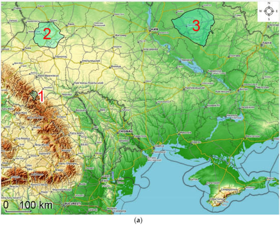
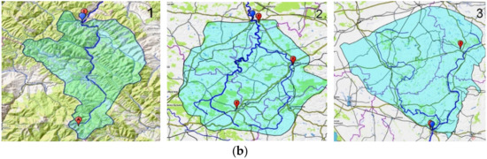
Figure 1.
The location of the catchment areas of the studied rivers (a), the hydrological (marked in blue) and meteorological (marked in red) stations (b): 1, the Prut–Yaremche, 2, the Styr–Lutsk, and 3, the Sula–Lubny. Note that the name of the catchment area includes the name of the river and the water gauge stations (catchment closing cross section).
In the upper course the Prut River up to the Yaremche hydrological station (with a catchment area of 597 km2) is a typical mountain river. Moreover, the source of the river is located near the Hoverla mountain, which is the highest in Ukraine (with an elevation of 2061 m) (Figure 1). A major part of the catchment area is covered by forests (primarily spruce). The climate of the catchment area of this river essentially depends on elevation. At the Pozhezhevska meteorological station, at a height of 1451 m a.s.l., the mean annual air temperature is equal to 3.5 °C, the mean air temperature in January is minus 5.8 °C, and the mean air temperature in August (the warmest month) is 13.3 °C. On the other hand, the air temperature at the Yaremche meteorological station (at an elevation of 531 m, near the Yaremche hydrological station) is significantly higher: in the period 1991–2020, the mean annual air temperature equalled 7.9 °C. The coldest month is January (minus 2.2 °C), and the warmest one is July (17.8 °C). Under cold conditions, the snow cover in the upper part of the mountains may persist until early June. The mean annual precipitation in the catchment area is above 1000 mm; at the Pozhezhevska meteorological station, it is 1548 mm; and at the Yaremche station, it is 1013 mm. There are waterfalls on the river, including the Probiy waterfall, several kilometres upstream from Yaremche hydrological station. At the same time, there is no pond or any other water reservoir upstream the station. The water regime of the Prut River depends mainly on the snow cover depth and heavy rains. As a rule, the largest river flow is observed in April, during the snow-melting season. Meanwhile, the largest water discharges are caused by heavy rains in the summer period. The main flow characteristics of the Prut River (Yaremche water gauge) are shown in Table 1.

Table 1.
The main characteristics of the discharge conditions of the studied rives, data modified, according to [55].
The Styr River is located in the north-western part of Ukraine (Figure 1). It is a tributary of the Pripyat River, and the Pripyat River is the largest tributary of the Dnipro River. The upper, southern part of the catchment area upstream features the town of Lutsk, on Volyn-Podilsk Upland, while the lower part is on the Polesian Lowland. The climate of the catchment area is moderate with cool winters and warm summers. During the period 1991–2020, the mean annual air temperature at the Lutsk meteorological station was equal to 8.5 °C; the mean air temperature in January was minus 2.9 °C, whereas in July, it was 19.7 °C. The air temperature at other stations, located upstream, was a little higher (by 0.1–0.2 °C). The precipitation in the catchment area upstream from the town of Lutsk amounts to an average of about 600–700 mm. The water regime of the Styr River at the Lutsk hydrological station (its catchment area is 7200 km2) is rather stable. The largest discharges observed in April and May are about twice as large as those observed at low water in August and September. In the upper course of the river, there are some reservoirs and many ponds. The reservoirs are rather small, and they do not significantly impact the water regime. The same can be said about ponds, many of which are older than 100 years. The main flow characteristics of the Styr River (Lutsk water gauge) are shown in Table 1.
The Sula River catchment is on the Dnipro Lowland with plain relief (north-east Ukraine), in the forest steppe zone, which actually has little forest (Figure 1). The climate of the catchment area is moderate, with cool winters and warm, sometimes hot, summers. During 1991–2020, the mean annual air temperature at the Lubny meteorological station was equal to 8.6 °C, the mean air temperature in January was minus 4.1 °C, and the mean air temperature in July was 21.3 °C. The air temperature at another station, Romny, located upstream, was lower by approximately 0.5 °C. The precipitation in the catchment area upstream from the town of Lubny amounts to an average of about 600 mm. The water regime of the river, comparable to the Styr River, is much more unstable. The mean discharges at the Lubny hydrological station (with a catchment area of 14,200 km2), observed in April and May, are approximately 10 times larger than those observed at low water in September. The flow regulation of the Sula River is small. The main flow characteristics of the Sula River (Lubny) are shown in Table 1.
2.2. Dataset Characteristics
The dataset consisted of the average monthly river flows, precipitation, and air temperatures from the period 1961–2020, acquired for three studied catchment areas. The monthly river-flow data were analysed for the Prut–Yaremche, the Styr–Lutsk, and the Sula–Lubny hydrological stations, and for the meteorological stations (Figure 1b), data on the average monthly air temperature and precipitation were analysed. For the Prut River basin, data were used from the Pozhezhevska meteorological station, in the upper part of the river basin, and from the Yaremche meteorological station, near the water gauge. For the Styr River catchment, data from three meteorological stations were used: Brodu (in the south), Dubno (in the east), and Lutsk( near the hydrological station). For the Sula River basin, data from the Romny (in the north-east part of the river catchment) and Lubny (in the south) meteorological stations were used. The time series consisted of the average monthly data for all points of observation.
2.3. Descriptive Statistics
Descriptive statistics of distribution of river-flow variables showed that the threshold values of skewness and kurtosis were exceeded (Table 2); therefore, for the purposes of further analysis, nonparametric measures of central tendency, i.e., Median (Quartiles 1–3), were used. As for the distribution of precipitation and air temperature, the skewness values did not exceed 2.0 and the kurtosis −7.0 (Table 3); hence, the nonparametric measures were used for further analysis (mean and standard deviation).
Table 2.
Descriptive statistics of river flow (m3/s) grouped for the period 1961–2020 (N = 720).
Table 3.
Global descriptive statistics of precipitation and air temperature grouped by river catchment area for the period 1961–2020 (N = 720).
Compared with the Prut and Styr rivers, the Sula River was characterized by a high standard deviation of monthly flows from the average value, which means that the monthly flows showed high variability over the analysed period (Table 2). The large variance in the flow series was also confirmed by the fact that the highest IQR (22.36) to median ratio (second quartile Q2) was also determined for the Sula–Lubny and the lowest for the Styr–Lutsk.
Table 3 shows that the catchment area of the Prut River had the highest mean precipitation (about 100 mm per month); for the other two rivers’ catchments, the precipitation was approximately 50 mm. The degree of variability was similar for all rivers and represented approximately 60% of the average value. The mean air temperature at the Yaremche station during 1961–2020 was about 7.4 °C, and for the other two rivers, the temperature was in the range 8.4–8.5 °C (Table 3). The degree of variability was similar for all rivers and was about 90–100% of the average value.
2.4. Forecast Algorithm
River-flow and meteorological variables forecasting was carried out in several stages, as shown in flowchart (Figure 2). The algorithm used allowed direct multistep-ahead forecasting with multiple (grouped or hierarchical) time series by using the built-in methods of the “R-forecast ML” package [56] inspired by Bergmeir et al. [57]. The applied direct forecasting approach included the following steps: (1) building a single multioutput model that simultaneously forecasts over short- and long-term forecast horizons, (2) assessing the generalization performance of the model over a variety of available data sets over time, and (3) selecting the hyperparameters that minimize forecast error over the relevant forecast horizons and re-train.
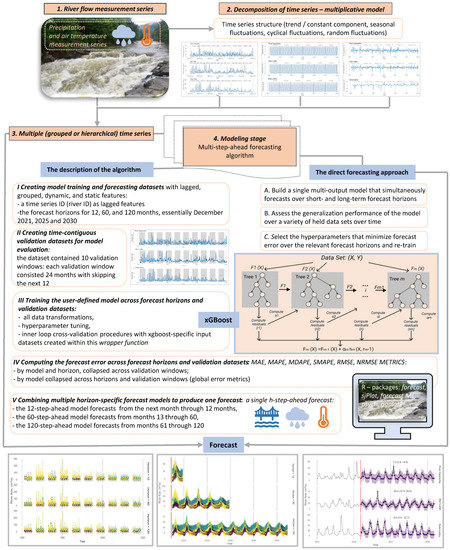
Figure 2.
General flowchart of a multistep-ahead forecasting algorithm.
The description of the algorithm is broken down into individual steps in Figure 2.
The first step was to create model training and forecasting datasets with lagged, grouped, dynamic, and static features. For this purpose, the create_lagged_df() function of the “R-forecast ML” package was used. The basic idea behind creating custom-feature lags was to improve model accuracy by removing noisy or redundant features in high-dimensional training data. For this purpose, three horizons were defined with forecasts for 1:12, 1:60, and 120 months into the future. A numerical vector indicating the lags in the dataset rows for the creation of the lagged features (lookback) was defined at levels of decreasing range (features from 1 to 36 months, from 54 to 78 months, and from 120 to 126 months in the past) with monthly frequency. The variables month and year were defined as dynamic variables with no static variables in the dataset. Based on multiple time series, the variable “river_id” identified the groups (hierarchies) that were used as model features but were not lagged. The same procedure was performed for the test data set in the model and forecast stage.
The next step involved creating time-contiguous validation datasets for model evaluation. Given that measurements are taken monthly, each validation window consisted of 24 months, skipping the next 12 months. As a result, the dataset contained 10 validation windows. Custom validation subsets with skipped river-flow data are shown in Figure S1 (Supplementary Materials). A similar approach was used for precipitation and air temperature.
Training the user-defined model across forecast horizons and validation datasets was carried out in the next step. The user-defined model consisted of all data transformations, hyperparameter tuning, and inner loop cross-validation procedures with XGBoost-specific [58] input datasets created within this wrapper function.
The next step involved computing the forecast error across forecast horizons and validation datasets (Figure S1 in Supplementary Materials). Estimating forecast error metrics on the test datasets was based on the calculation of the following: mean absolute error (MAE), mean absolute percentage error (MAPE), median absolute percentage error (MDAPE), symmetrical mean absolute percentage error (SMAPE), root mean squared error (RMSE), and normalized root mean squared error by standard deviation (NRMSE), which have been discussed in detail in the works of, i.a., Bahrami-Pichaghchi and Aghelpour [59], and Aghelpour and Norooz-Valashedi [60].
The final step involved combining the multiple direct-horizon forecast models to produce a single h-step-ahead forecast. Prediction intervals were estimated by calculating the α/2 and 1-α/2 percentiles of the simulated data for each prediction horizon by using bootstrap residuals and recursive multivariate prediction. The one-step-ahead prediction error was defined as:
where represents the actual prediction, represents the prediction conditioned by previous prediction, ϵ represents the estimation error predictions, which were simulated by including the residuals (sampling from the collection of errors from past prediction iterations). The expected variance was represented by the difference in predictions.
The approach was to combine forecasts across models in such a way that short-term models would produce short-term forecasts and long-term models would produce long-term forecasts. This implies that for 120 months, the ahead forecast included (1) the 12-step-ahead model forecasts from the next month through 12 months, (2) the 60-step-ahead model forecasts from months 13 through 60, and (3) the 120-step-ahead model forecasts from months 61 through 120.
Analyses were performed with the statistical language R (version 4.1.1) [61].
XGBoost Algorithm
For modelling and forecasting river flows and meteorological variables, an XGBoost was chosen as it outperforms other machine-learning (ML) algorithms, such as artificial neural networks (ANN) or support vector regression (SVR), and statistical models in the case of a multilevel predictive average [62]. The process is called gradient boosting because it makes use of an algorithm to minimize losses when adding new models (Figure 3). Training is an iterative process: new trees are added that predict the residuals or errors of the previous trees, and they are subsequently combined with the previous trees to make the final prediction. XGBoost minimizes a regularized (L1 and L2) objective function that combines a convex loss function (based on the difference between predicted and target outputs) and a penalty term for model complexity.
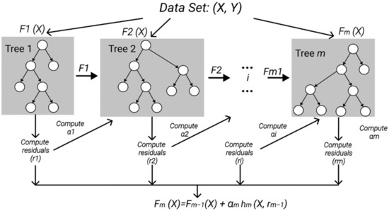
Figure 3.
Schematic principle of the XGBoost algorithm for the training process (the figure was prepared on the basis of XGBoost documentation [63]).
In Figure 3, αi and ri are regularization parameters and residuals computed in the ith tree separately. Here, hi is a function that is trained to predict results, and ri uses X for the ith tree.
To compute αi, the computed residuals used ri and estimated the following:
where L (Y, F (X)) is a differentiable loss function. , where represents the training loss function, represents model parameters, y represents the actual value, and represents the predicted value.
Using a sampling procedure, 80% of the sample was qualified for the training set and 20% for the test set. The training of the model was performed by using eXtreme Gradient Boosting Training with the following parameters of tree booster: maximum depth of a tree = 3; number of threads = 2; maximum number of boosting iterations = 20; control the learning rate ϵ = 0.3; minimum loss reduction required to make a further partition on a leaf node of the tree γ = 0.5; minimum sum of instance weight (hessian) needed in a child = 5; and evaluation metric rmse. For task parameters, the regression with squared loss was used as an objective function with early stopping rounds = 5. The regression with squared loss is referred to as:
where represents the training loss function, represents model parameters, y represents the actual value, represents the predicted value.
3. Results
3.1. River-Flow Dynamics in Relation to Changes in Precipitation and Air Temperature over the Decades 1961–2020
For a graphical representation of the flow distribution during the study period, see Figure 4. From the data provided, one can follow the dynamics of flow over the decades. In the case of the Prut River at the Yaremche station, variable dynamics was evident over the study period. The smallest values of flow were recorded in the period 1960–1970, the largest in the period 2000–2010. In the last decade, a significant decrease in flow was observed at the level of the local minimum for 50 years (median = 8.0 m3/s). A similar situation was observed in the case of the Styr River (Lutsk water gauge), where the maximum flow values recorded over 2000–2010 changed into the minimum flows during the entire observation period recorded over 2010–2020. In the last decade, the median was 23.7 m3/s (with the median of 26.9 m3/s for the period 1961–2020), which is 7.1 m3/s lower than that in the 2000–2010 decade. Similarly, in the case of the Sula River (Lubny water gauge), the period of increase in the flow between 1960 and 1990 was followed by a continuous decline, with a global minimum recorded in the last decade.
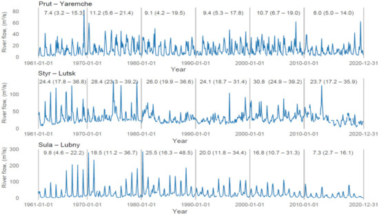
Figure 4.
Flow time series distribution grouped by rivers (1961–2020). Note that figure descriptions refer to the nonparametric measures of central tendency—median (Quartile 1–Quartile 3).
The trend dynamics of river-flow amounts over the decades is shown in Figure 5. In the case of the Prut–Yaremche, an alternating trend was observed, with periods of growth (1960–1980, 1990–2010) alternating with periods of decline (1980–1990, 2010–2020). The last decade was characterized by the sharpest decline during the study period, when the flow reached the global minimum. A similar situation was observed in the case of the Styr–Lutsk, where the flow decreased by more than 25% in 2010–2020. In the case of the Sula–Lubny, the period of increase in flow (1960–1990) was followed by a period of decrease at the end of the study period, when the global flow minimum was reached in 2010–2020.
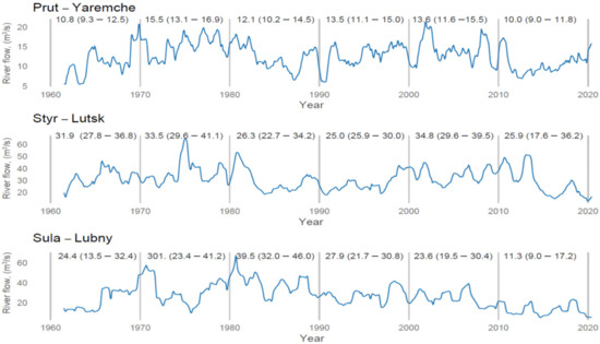
Figure 5.
Flow trend values grouped by rivers (1961–2020). Note that figure descriptions refer to nonparametric measures of central tendency—median (Quartile 1–Quartile 3).
The seasonal component is the same for all rivers, the only difference being its variability. The lowest variability (0.3) was observed in the case of the Styr River at Lutsk, whereas the highest in the case of the Sula–Lubny (0.9). The dynamics of the seasonal component of river flows in the period 1961–2020 is shown in Figure S2 (in Supplementary Materials). The level of the random component was similar for all rivers. Variability in the case of rivers Prut–Yaremche and Sula–Lubny was also similar, but it was lower for the Styr River at Lutsk. In all cases, a slow decline in the average component and variability was observed throughout the study period, with local or global minima in the last decade, except the Sula–Lubny, where a wave of variation was observed. The dynamics of the random component of river flow is shown in Figure S3. In the case of the Prut River catchment, the lowest precipitation was recorded between 1980 and 1990, and it was followed by an increase in precipitation with a global maximum observed in the last decade 2010–2020 (Figure S4). In the case of the Styr River catchment, a slight variation in the dynamics of precipitation was observed: the period of increasing precipitation alternated with the period of decreasing precipitation. In the Sula River catchment, following a clear increase in precipitation in the 1970s and a corresponding stable level during the next 40 years, a decrease in precipitation below 50 mm was recorded in 2010–2020, which corresponds to the local minimum for 50 years.
The trend dynamics of precipitation amounts over the decades is shown in Figure S5 (in Supplementary Materials). The precipitation data indicate that in the case of the Prut River catchment, the declining trend period in the 1960s–1990s was replaced by an increasing trend with the global maximum in the last decade of the study period. In the case of the Styr River at Lutsk, there was a slight variation in the trend over the period with increases/decreases during one or two decades with the global average at the end of the study period. In the Sula River catchment, maximum values of the precipitation trend were observed in the period 1970–2000, which was followed by a period of a downward trend with a local minimum in the last decade of the study period. The seasonal component is the same for the Prut River and the Styr River catchments. With the same average seasonality, the Sula River catchment was characterized by the lowest variability of the three rivers. The dynamics of the seasonal component of precipitation is demonstrated in Figure S6. The mean of the random component was the same for all the rivers’ catchments, the degree of variability increasing slightly in the second half of the study period, reaching local or global maxima. The lowest variability was observed for the Prut River and the highest for the Sula River catchment. The dynamics of the random component of precipitation is demonstrated in Figure S7.
For all three river catchment areas, the lowest average air temperatures were recorded in the first decade of the study period. The study period was characterized by an almost-continuous increase in average air temperatures. The value of the increase ranged from 1.6 °C to 2.1 °C with global maxima in the last decade (Figure S8 in Supplementary Materials). The trend dynamics of air temperature over the decades is presented in Figure S9. The data show a continuous upward trend for each river’s catchment from the beginning of the observation to the end of the study period. Global trend maxima were reached in the last decade. The degree of variability for all river catchments was characterized by a period of increase, with the maximum in the period 1980–1990, followed by a decrease in variability to local or global minima. The seasonal component of air temperature was the same for the Prut River and Styr River catchments. With the same average seasonality, the Prut River catchment was characterized by the lowest variability (Figure S10). The level of the random component was similar for all the rivers’ catchments, the variability was also similar (Figure S11). In all cases, a slow decline in the average component and variability was observed throughout the study period, with global minima in the last decade.
3.2. Forecasting Monthly River Flows and Meteorological Variables
River-flow, precipitation, and air temperature forecasting was performed in three stages: using train (80%) and test (20%) subsets, using a model with train-test data, and training with all data.
3.2.1. River-Flow Forecasting
The fitting of the data within the selected validation subgroups is presented in Figure S12 (in Supplementary Materials), where the dashed lines represent the actual data not fitted by the model. Measures of data fit in terms of prediction errors can be found in Tables S1 and S2 (in Supplementary Materials). The data show that the fitting errors are quite large. This is best seen in the normalized RMSE (NRMSE), which was calculated as the ratio of the RMSE to the global SD of flow for each river, separately. Global NRMSE values of 0.78, 0.82, and 0.61 tell us that the model does not fit the data well enough to trust such predictive results (>0.5), but it is better than the usual data randomization based on global M and SD (<1). The absence of the overfitting and underfitting (the RMSE value is similar at each fitting step for the training and test sets) of the data is evidence for judiciously selecting model parameters. A significant RMSE value at each fitting step indicates high variability in the data that cannot be reasonably well fitted by retrospective data, regardless of the selected horizon length.
Given the above limitations, the prediction of river flow for the next approach was performed by using the training set and the test set for individual rivers in periods of 12, 60, and 120 months. The aggregated prediction plots are shown in Figure 6.
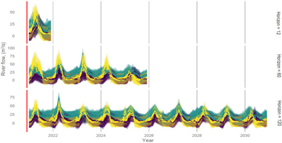
Figure 6.
12-, 60-, and 120-step-ahead forecasts of river flows (purple line: the Prut–Yaremche, turquoise line: the Styr–Lutsk, yellow line: the Sula–Lubny).
The predictions of river flow within each horizon are shown in Table 4.
Table 4.
Forecast by river-flow model with train-test data grouped by horizon.
An analogous prediction was made, taking into account all the data in the form of a test set. Figure 7 shows combined multiple direct-horizon forecast models for producing a 120-month step-ahead forecast grouped by “river id”.
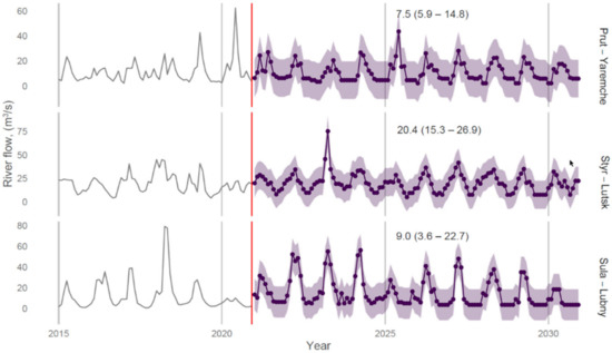
Figure 7.
Combined plot with partial actual data (2015–2020) and predicted data (2021–2030) for the river-flow model trained with all data. Explanations: The left side of the graph shows a portion of the actual data (2015–2020) and the red vertical bar shows the boundaries of the actual data and the beginning of the forecast data. The data in purple represents the forecast data. The purple circles reflect the values with a monthly step, and the filled background represents the prediction intervals.
The predictions for the entire set are essentially consistent with the predictions in Table 4. Based on the results given in Figure 7, it can be concluded that the flow level of the Prut–Yaremche will remain the same or will decrease by about 6% in the period 2021–2030 (compared with the flow level in the period 2010–2020). In the case of the Styr River at Lutsk, the flow level will decrease by about 12–14%. In contrast, the flow of the Sula–Lubny in 2021–2030 is expected to be 1.2–1.7 m3/s higher than in 2010–2020, which corresponds to a projected increase of 16–23%.
3.2.2. Precipitation Forecasting
In the case of precipitation forecasting, the fitting of the data within the selected validation subgroups is shown in Figure S13 (in Supplementary Materials), where the dashed lines represent the actual data not fitted by the model.
The data in Tables S3 and S4 (in Supplementary Materials) show that the fitting errors of prediction are quite large. This is best seen in the normalized RMSE (NRMSE), which was calculated as the ratio of the RMSE to the global SD of precipitation for each river catchment, separately. Global NRMSE values of 0.79, 0.86, and 0.96 indicate that the model does not fit the data well enough to trust such predictive results (>0.5) but are better than the usual data randomization based on global M and SD (<1). The absence of the overfitting and underfitting of the data (the RMSE value is similar at each fitting step for the training and test sets) is evidence for judiciously selecting model parameters.
Given the above limitations, as in the case of river-flow forecasting, precipitation forecasting using the training set and the test set approach were performed for individual rivers in periods of 12, 60, and 120 months. The aggregated forecast plots are shown in Figure S14. The predictions of precipitation values within each horizon are shown in Table 5.
Table 5.
Forecast by precipitation model with train-test data grouped by horizon.
An analogous prediction (as for river-flow forecast) was made, taking into account all the data in the form of a test set. Precipitation predictions for the 120-month period for each river catchment are shown in Figure 8.
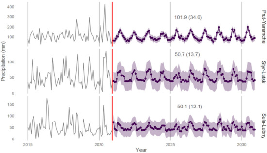
Figure 8.
Combined plot with partial actual data (2015–2020) and predicted data (2021–2030) for the precipitation model trained with all data. Explanations are the same as those for Figure 7.
Based on the results provided in Figure 8, it can be concluded that in the period 2021–2030, the amount of precipitation in the Prut River catchment will decrease by about 7–10% (compared with the precipitation level in 2010–2020). In the case of the Styr River catchment, the amount of precipitation will remain at the level of the last decade or slightly decrease (by 1–2 mm). For the Sula River basin, the forecast shows an increase in average precipitation (by 1–3 mm) compared with the last decade.
3.2.3. Air Temperature Forecasting
In air temperature forecasting, the fitting of the data within the selected validation subgroups is shown in Figure S15 (in Supplementary Materials), where the dashed lines represent the actual data, almost all of which were fitted by the model.
The data in Tables S5 and S6 (in Supplementary Materials) show that the fitting errors of prediction were rather moderate. This is best seen in the normalized RMSE (NRMSE), which was calculated (similar to river flows and precipitation) as the ratio of the RMSE to the global SD of temperature for each river, separately. Global NRMSE values of 0.28–0.30 tell us that the model provides a 3.3–3.5 times better prediction of the data than in the case of the usual data randomization based on global M, SD. A low RMSE value at each fitting step indicates that the data can be reasonably well fitted by retrospective data, regardless of the horizon length chosen.
Given the above limitations, air temperature forecasting for the approach with the training set and the test set was performed for individual rivers in periods of 12, 60, and 120 months. The aggregated forecast plots are shown in Figure S16.
The predictions of air temperature values within each horizon are shown in Table 6.
Table 6.
Forecast by air temperature model with train-test data grouped by horizon.
An analogous prediction was made taking into account all the data in the form of a test set. Air temperature predictions for the 120-month period for each river catchment are shown in Figure 9.
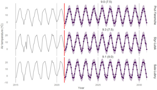
Figure 9.
Combined plot with partial actual data (2015–2020) and predicted data (2021–2030) for the air temperature model trained with all data. Explanations are the same as those for Figure 7.
Based on the results provided in Figure 9, it can be concluded that the air temperature in each individual river basin will increase by 0.1 °C to 0.4 °C. In the case of the Styr River and the Sula River catchments, a trend of further variability decrease is observed. Air temperature variability for the Prut River basin will remain unchanged in the period 2021–2030.
4. Discussion
The results of the monthly flow forecasts made for three rivers in Ukraine show a different fit of the model to the data, which is underlined by the measures of the model’s performance. To some extent, similar patterns of the long-term variability of the monthly flow were obtained. However, forecasts of flows were different, which to a greater or lesser extent is related to the multiyear variability and different forecasts of precipitation and air temperature.
4.1. Long-Term Changes of Monthly River Flow under Different Precipitation and Air Temperature Conditions
In all the studied rivers, a variable dynamic of flows was observed in the years 1961–2020, with a clearly marked decrease in monthly flows in the last decade of 2010–2020. The last decade of low flows on the Prut–Yaremche and the Styr–Lutsk rivers was preceded by their noticeable increase in the earlier 2000–2010 decade. On the other hand, in the case of the Sula–Lubny river, a continuous decrease in monthly flows had been observed since the end of the 1990s (after a 30-year period of flow increase since the beginning of the 1960s) with a global minimum in the 2010–2020 decade. These changes are confirmed by the dynamics of flow trends, showing alternating periods of increase and decrease in flows over the decades of the analysed multiannual period (Figure 5).
The variability of river flows is partly related to the trends of precipitation and air temperature in the studied catchments. The decrease in flows observed on the Prut River in 1980–1990 corresponds to the lowest precipitation recorded in the 1980s–1990s. On the other hand, the observed small increase in precipitation during 1961–2020 was accompanied by a small decrease in river flow. One of the reasons for this discrepancy was a significant increase of air temperature and a corresponding increase of evaporation from the catchment area, which is also documented by the research of Vyshnevskyi and Donich [53]. Similar tendencies of climate parameters and river-flow changes were obtained for the Styr and the Sula rivers. Despite a small increase of precipitation, water runoff tends to decrease. This decrease is bigger than that of the Prut River. In our opinion, such decrease of flow of plain rivers may be explained by two factors: an increase of water intake during warm weather (in particular due to the irrigation of farming land) and an increase of evaporation from ponds and reservoirs. As shown in the paper by Vyshnevskyi [64], the dependence between evaporation and air temperature is nonlinear: a small increase in air temperature results in a significant increase of evaporation.
For all the studied rivers, a similarity was identified in the seasonal fluctuation component and the level of the random component of monthly flows. A detailed analysis of random flow fluctuations for selected rivers has not been carried out; therefore, research on these issues should be continued in the future.
4.2. Forecasting of Monthly River Flow with Precipitation and Air Temperature Forecasts
Results of the forecasts for 2021–2030 for the studied catchments showed that the dominant pattern is as follows: a decrease in flows is accompanied by a decrease in precipitation and an increase in air temperature (the Prut and the Styr). The differences relate to the magnitude of the flow change of approximately 6% compared with the 2010–2020 decade for the mountainous Prut River (or even no change in flow) and about 14% for the Styr River, predominantly in the uplands. On the other hand, the forecasts for the Sula River provide for an increase in flows (16–23%), with an increase in precipitation and air temperature, which is what makes it different from other rivers. It may be assumed that with an increase in precipitation in the Sula River catchment area, soil retention (underground retention) will also become more important in shaping the river flows, which will contribute to levelling the differences between high spring flows and low summer–autumn flows. The predicted changes in the flows of the Prut, the Styr, and the Sula rivers correspond to the forecasts in other regions of Ukraine and Europe. Over the past decades, climate change has been observed in Europe, and it has been emphasized that these changes will be stronger in the future [65,66,67,68,69,70]. Many studies on the impact of climate variability and change on water resources in Europe, using hydrological models on a continental and global scale, predict lower flows, with increasing air temperature and lower or no significant changes in precipitation [71,72,73,74]. However, the various types of changes are not evenly distributed either in time or in space. Didovets et al. [69] analysed changes in precipitation and temperature until the end of the 20th century in the catchment areas of Ukraine and determined their impact on the water availability of main river basins by using global hydrological models, which were compared with global climate models (GCM) in two representative concentrations pathways scenarios: RCP 2.6 and RCP 8.5. A historical period (1971–2000) and two future periods (2041–2070 and 2071–2100) were considered, showing that changes in mean annual precipitation range between −14% and +10% and changes in the mean annual river discharge range from −30% to +6%, depending on RCP. The largest decrease in the mean annual runoff was forecast for the Pripyat, the Southern Bug, and the Dniester basins, reaching up to −30% by the end of the century in RCP 8.5, which was also confirmed by the present current study for the Styr River, which is a tributary of the Pripyat River.
4.3. Assessment of the Forecasts of Monthly River Flow
In the present research (regarding the Prut, Styr, and Sula rivers), attention was drawn to a significant RMSE value at each fitting step, which indicates high variability of the data that cannot be reasonably well fitted by retrospective data, regardless of the selected horizon length. This leads to the conclusion that the monthly data frequency for flow is too low to produce good fitting results and that it is worthwhile to use the daily frequency. Comparing the obtained results with other forecasts yields an emphasis on the fact that uncertainty regarding the forecasting of hydrological characteristics is still high, regardless of the location of the rivers and the adopted research methods. The variability of the river-flow time series can be influenced by various parameters, such as air temperature, precipitation, and evaporation, which makes accurate estimations and predictions of the flow almost impossible, the more so as it is further complicated by complexity, nonstationarity, and the nonlinearity of the river-flow phenomenon [75,76,77].
An analysis of the homogeneity and stationarity of an average monthly flows of Ukrainian rivers (305 water gauge stations, from the beginning of the observation until 2010), carried out with the use of hydrogenetic methods [78], has shown that most of the observation series are homogeneous and stationary. The exceptions include rivers with significant anthropogenic impact (river regulations, water intakes, deforestation, etc.). Observation series with a full cycle of long-term cyclic fluctuations (dry and wet phase) are stationary, whereas other observation series are quasistationary. Many studies indicate a large diversity of predictions and forecasts, especially those obtained for large rivers (often transboundary) and a high uncertainty as to the predicted hydrological effects in the future due to the visible climate changes and their impact on the hydrological characteristics of rivers, also in Ukraine [15,78]. The importance of studies on the strength of simulated changes and the effects on river flows has also been confirmed [79,80,81,82].
A staged forecasting process used in this study takes into account the gradient enhancement approach of the XGBoost model. In the approach applied to Ukrainian rivers, a single multioutput model was proposed that simultaneously forecasts over short- and long-term horizons. The generalization performance of the model over a variety of available data sets over time was assessed, and the hyperparameters which minimize the forecast error over the relevant forecast horizons were selected. The algorithm used allowed direct multistep-ahead forecasting with multiple time series (grouped or hierarchical) inspired by Bergmeir et al. [57]. As suggested by Sanders et al. [41] and Osman et al. [83], XGBoost models use all input data directly, without any preprocessing or selection, and a proper selection of the input fields is essential to improve the performance of XGBoost models. Usually, unavoidable errors may result from introduced model limitations or the nonstationarity of hydrological processes [84]. An additional difficulty may be the quality of hydrological and meteorological data, another being the calibration of parameters [85,86]. Yang et al. [87] suggest including additional hydrological information in river-flow forecasts to improve model performance. On the other hand, research conducted by Sanders et al. [41] shows that using more information on the catchment area and data from point measurements can lead to a reduction in the performance of forecasting models. According to Aghelpour et al. [88], consideration of the climatic indices (e.g., Southern Oscillation Index, Global Mean Temperature Index, North Pacific pattern, Pacific Decadal Oscillation, North Atlantic Oscillation) as inputs in prediction models of river flows in Iran may improve monthly flow prediction by 24% on average.
Complex river-flow prediction models typically require multiple hydrological and climatological parameters as input, many of which may not be available for some locations, and the complexity of the flow processes makes it difficult to use physical models. Many estimates and forecasts of river flows have well documented that combined models (hybrid models) may show better performance compared with stand-alone models [89,90,91].
5. Conclusions
Long-term changes were estimated, and a forecast of monthly river flows was made for three rivers (the Prut, the Styr, and the Sula) in Ukraine with reference to the variability and forecasts of precipitation and air temperature. The years 1961–2020 were selected as the historical period, while the forecast horizons of 12, 60, and 120 months into the future were specified for this dataset, i.e., December 2021, December 2025, and December 2030.
The forecasting of monthly river flows was carried out in three stages with the use of input data sets characteristic for the XGBoost algorithm: train (80%) and test subsets (20%), using a model with train-test data, and forecasting by training with all data for forecast horizons (December 2021, December 2025, and December 2030). The adoption of this algorithm allowed direct multistep-ahead forecasting with multiple (grouped or hierarchical) time series, which may be of importance taking into account sometimes-scarce measurements of daily river flows. This is one of the main advantages and a new, unique feature of the adopted forecasting method, which is characterized by high versatility of use, regardless of the spatial location of the river catchment areas. The direct forecasting approach used included the following steps: build a single multioutput model that simultaneously forecasts over short- and long-term forecast horizons, assess the generalization performance of the model over a variety of held data sets over time, and select the hyperparameters that minimize forecast error over the relevant forecast horizons and re-train.
The selected rivers flow through different physical geographical and climatic regions and represent different hydrological systems: the Prut, a mountain river; the Styr, an upland river; and the Sula, a lowland river. These features undoubtedly influenced their different degree of sensitivity and resistance to variability of climatic conditions and possible anthropogenic influences. The conducted analysis showed some differences in the trends of changes in monthly flows in individual decades of the period 1961–2020 and similarities in terms of the seasonal component and random flow fluctuations. An emphasis was put on the last decade, significant for future forecasts, in which a decrease in flow was determined for the Prut and the Styr rivers, whereas an increase was determined for the Sula River. Two patterns were obtained in the forecasts, which partially correspond to the results of flow forecasts obtained for Ukrainian rivers with the use of other methods and models. A decrease in flow, accompanied by a decrease in precipitation and an increase in air temperature until 2030, are expected according to the forecasts for the Prut and Styr rivers, whereas for the Sula River, the forecasts assume an increase in flow, accompanied by an increase in precipitation and air temperature.
The advantages of the model used for forecasting of monthly river flows in Ukraine, i.e., modelling many time series simultaneously using one model, include the simplicity of modelling, potentially more-robust results because of pooling data across time series, and solving the “cold start” problem when few data points are available for a given time series. Unlike the recursive or iterative method of creating forecasts in multiple steps used in traditional forecasting (such as ARIMA), direct forecasting involves creating a series of distinct, horizon-specific models. Although there are several hybrid methods for creating multistep forecasts, the simple, direct forecasting method used avoids the exponentially more-difficult problem of “predicting the predictors” for forecast horizons beyond one step in the future.
The obtained results of the forecasts, although approximate to some extent, provide information on future (in the next decade) changes in monthly flows of Ukrainian rivers (the Prut, the Styr, and the Sula) occurring under various environmental and climatic conditions, and they highlight the need to extend research into assessments of the impact of anthropogenic factors on the long-term dynamics of changes in river flows. In future studies of the daily flows, precipitation and air temperature should test the effectiveness of multistage forecasting with multiple, grouped, or hierarchical time series in the forecasting of hydrological and meteorological parameters. The research results can be used for the management and rational planning of water resources in the studied regions of Ukraine. They can provide the basis for the rational use of river water resources, such as for irrigation purposes, which is certainly a great challenge in the situation of increasingly frequent and longer periods of drought.
Supplementary Materials
The following supporting information can be downloaded at: https://www.mdpi.com/article/10.3390/resources11120111/s1, Figure S1. Custom validation subsets (grey areas) with skipped data (white areas) for river flow, Figure S2. Seasonal flow values grouped by rivers (1961–2020), Figure S3. Random flow values grouped by rivers (1961–2020), Figure S4. Precipitation time series distribution grouped by rivers’ catchment areas (1961–2020). Note: Figure descriptions refer to non-parametric measures-mean (standard deviation), Figure S5. Precipitation trend values grouped by rivers (1961–2020), Figure S6. Precipitation seasonal values grouped by rivers (1961–2020), Figure S7. Precipitation random values grouped by rivers (1961–2020), Figure S8. Air temperature time series distribution grouped by rivers’ catchment areas (1961–2020). Note: Figure descriptions refer to non-parametric measures-mean (standard deviation), Figure S9. Air temperatur trend values grouped by rivers (1961–2020), Figure S10. Air temperatur seasonal values grouped by rivers (1961–2020), Figure S11. Air temperatur and random values grouped by rivers (1961–2020), Figure S12. River flows predicted (solid line) vs. actual (dashed line) values grouped by horizons (purple line: the Prut River-Yaremche, turquoise line: the Styr River–Lutsk, yellow line: the Sula River-Lubny), Figure S13. Precipitation predicted (solid) vs. actual (dashed) values grouped by horizons (purple line: Prut River catchment. turquoise line: Styr River catchment. yellow line: Sula River catchment), Figure S14. 12, 60 and 120 step-ahead forecasts of precipitation (purple line: the Prut River catchment, turquoise. line: the Styr River catchment, yellow line: the Sula River catchment), Figure S15. Air temperature predicted (solid) vs. actual (dashed) values grouped by horizons (purple line: PrutRiver catchment. turquoise line: Styr River catchment. yellow line: Sula River catchment), Figure S16. 12, 60 and 120 step-ahead forecasts of air temperature (purple line: the Prut River catchment, turquoise line: the Styr River catchment, yellow line: the Sula river catchment). Table S1. Forecast error by river flow forecast horizon, Table S2. Global river flow forecast error, Table S3. Forecast error by precipitation forecast horizon and river catchment, Table S4. Global precipitation forecast error grouped by river catchment, Table S5. Forecast error by air temperature forecast horizon and river catchment, Table S6. Global air temperature forecast error grouped by river catchment.
Author Contributions
Conceptualization, R.G. and V.V.; methodology, R.G.; software, R.G.; data curation, V.V.; writing—original draft preparation, R.G. and V.V.; investigation, R.G.; validation, R.G.; visualization, R.G.; writing—reviewing and editing, R.G. and V.V.; discussion, R.G. and V.V.; supervision, R.G. All authors have read and agreed to the published version of the manuscript.
Funding
This research received no external funding.
Data Availability Statement
The source of data derives from the measurement and observation data of the Hydrometeorological Service in Ukraine.
Acknowledgments
The authors thank their universities for their support. The authors would also like to acknowledge the Hydrometeorological Service in Ukraine for the release of the input database.
Conflicts of Interest
The authors declare no conflict of interest.
References
- Shmueli, G. To explain or to predict? Stat. Sci. 2010, 25, 289–310. [Google Scholar] [CrossRef]
- Blöschl, G.; Bierkens, M.F.P.; Chambel, A.; Cudennec, C.; Destouni, G.; Fiori, A.; Kirchner, J.W.; McDonnell, J.J.; Savenije, H.H.G.; Sivapalan, M.; et al. Twenty-three Unsolved Problems in Hydrology (UPH)–a community perspective. Hydrol. Sci. J. 2019, 64, 1141–1158. [Google Scholar]
- Papacharalampous, G.A.; Tyralis, H.; Koutsoyiannis, D.; Montanari, A. Quantification of predictive uncertainty in hydrological modelling by harnessing the wisdom of the crowd: A large-sample experiment at monthly timescale. Adv. Water Resour. 2020, 136, 103470. [Google Scholar] [CrossRef]
- Montanari, A. Hydrology of the Po River: Looking for changing patterns in river discharge. Hydrol. Earth Syst. Sci. 2012, 16, 3739–3747. [Google Scholar] [CrossRef]
- Steirou, E.; Gerlitz, L.; Apel, H.; Sun, X.; Merz, B. Climate influences on flood probabilities across Europe. Hydrol. Earth Syst. Sci. 2019, 23, 1305–1322. [Google Scholar] [CrossRef]
- Hussain, F.; Wu, R.-S.; Wang, J.-X. Comparative Study of Very Short-Term Flood Forecasting Using Physics-Based Numerical Model and Data-Driven Prediction Model. Nat. Hazards 2021, 107, 249–284. [Google Scholar] [CrossRef]
- Yaseen, Z.M.; Ebtehaj, I.; Bonakdari, H.; Deo, R.C.; Mehr, A.D.; Melini, W.H.; Mohtar, W.; Diop, L.; El-shafie, A.; Singh, V.P. Novel approach for streamflow forecasting using a hybrid ANFIS-FFA model. J. Hydrol. 2017, 554, 263–276. [Google Scholar] [CrossRef]
- Tu, H.; Wang, X.; Zhang, W.; Peng, H.; Ke, Q.; Chen, X. Flash Flood Early Warning Coupled with Hydrological Simulation and the Rising Rate of the Flood Stage in a Mountainous Small Watershed in Sichuan Province, China. Water 2020, 12, 255. [Google Scholar] [CrossRef]
- Sivakumar, B.; Jayawardena, A.W.; Fernando, T.M.K.G. River flow forecasting: Use of phase-space reconstruction and artificial neural networks approaches. J. Hydrol. 2002, 265, 225–245. [Google Scholar] [CrossRef]
- Chau, K.W. A split-step particle swarm optimization algorithm in river stage forecasting. J. Hydrol. 2007, 346, 131–135. [Google Scholar] [CrossRef]
- Abbas, S.A.; Xuan, Y. Development of a new quantile-based method for the assessment of regional water resources in a highly-regulated river basin. Water Resour. Manag. 2019, 33, 3187–3210. [Google Scholar] [CrossRef]
- Shen, C.; Laloy, E.; Elshorbagy, A.; Albert, A.; Bales, J.; Chang, F.-J.; Ganguly, S.; Hsu, K.-L.; Kifer, D.; Fang, Z.; et al. HESS Opinions: Incubating Deep-Learning-Powered Hydrologic Science Advances as a Community. Hydrol. Earth Syst. Sci. 2018, 22, 5639–5656. [Google Scholar]
- Hu, C.; Wu, Q.; Li, H.; Jian, S.; Li, N.; Lou, Z. Deep Learning with a Long Short-Term Memory Networks Approach for Rainfall-Runoff Simulation. Water 2018, 10, 1543. [Google Scholar] [CrossRef]
- Siuta, T.J. Modelowanie serii czasowych przepływów w krótkoterminowej prognozie hydrologicznej. Acta Sci. Polonorum. Form. Circumiectus 2020, 19, 3–14. [Google Scholar] [CrossRef]
- Khrystiuk, B.; Gorbachova, L. Long-term Forecasting of Extraordinary Spring Floods by Commensurability Method on the Dnipro River Near Kyiv City, Ukraine. J. Environ. Res. Eng. Manag. EREM 2019, 75, 74–81. [Google Scholar]
- Abrahart, R.S.; See, L. Multi-model data fusion for River flow forecasting; an evaluation of six alternative methods based on two contrasting catchment. Hydrol. Earth Syst. Sci. 2002, 6, 655–670. [Google Scholar] [CrossRef]
- Zeynoddin, M.; Bonakdari, H.; Azari, A.; Ebtehaj, I.; Gharabaghi, B.; Riahi Madavar, H. Novel hybrid linear stochastic with non-linear extreme learning machine methods for forecasting monthly rainfall a tropical climate. J. Environ. Manag. 2018, 222, 190–206. [Google Scholar] [CrossRef]
- Peng, Z.; Zhang, L.; Yin, J.; Wang, H. Commensurability-Based Flood Forecasting in Northeastern China. Pol. J. Environ. Stud. 2017, 26, 2689–2702. [Google Scholar] [CrossRef][Green Version]
- Apel, H.; Thieken, A.H.; Merz, B.; Blöschl, G. Flood risk assessment and associated uncertainty. Nat. Hazards Earth Syst. Sci. 2004, 4, 295–308. [Google Scholar] [CrossRef]
- Khrystiuk, B.F. The forecasting of the average, maximum and minimum for a ten-day period of water discharges on Upper Danube. Proc. Ukr. Hydrometeorol. Inst. 2012, 262, 206–220. (In Ukrainian) [Google Scholar]
- Khrystiuk, B.; Gorbachova, L.; Koshkina, O. The impact of climatic conditions of the spring flood formation on hydrograph shape of the Desna River. Meteorol. Hydrol. Water Manag. 2017, 5, 63–70. [Google Scholar] [CrossRef]
- Shevnina, E. Methods of long-range forecasting of dates of the spring flood beginning and peak flow in the estuary sections of the Ob and Yenisei rivers. Russ. Meteorol. Hydrol. 2009, 34, 51–57. [Google Scholar] [CrossRef]
- Scitovski, R.; Maričić, S.; Scitovski, S. Short-term and long-term water level prediction at one river measurement location. Croat. Oper. Res. Rev. (CRORR) 2012, 3, 80–90. [Google Scholar]
- Sharma, P.; Machiwal, D. Streamflow forecasting. In Advances in Streamflow Forecasting; Sharma, P., Machiwal, D., Eds.; Elsevier: Amsterdam, The Netherlands, 2021; pp. 1–50. [Google Scholar]
- Toth, E.; Brath, A.; Montanari, A. Comparison of short-term rainfall prediction models for real-time flood forecasting. J. Hydrol. 2000, 239, 132–147. [Google Scholar] [CrossRef]
- Imrie, C.E.; Durucan, S.; Korre, A. River flow prediction Rusing artificial neural networks: Generalisation beyond the calibration range. J. Hydrol. 2000, 233, 138–153. [Google Scholar] [CrossRef]
- Ozgur, K. River Flow Modeling Using Artificial Neural Networks. J. Hydrol. Eng. 2004, 9, 60–63. [Google Scholar]
- Teschl, R.; Randeu, W.L. An Artificial Neural Networkbased Rainfall-Runoff Model Using Gridded Radar Data. In Proceedings of the Third European Conference on Radar in Meteorology and Hydrology (ERAD), Visby, Sweden, 6–10 September 2004. [Google Scholar]
- Krzanowski, S.; Wałęga, A. Zastosowanie sztucznych sieci neuronowych do predykcji szeregów czasowych stanów wody i przepływów w rzece. Acta Sci. Pol. Form. Circumiectus 2007, 6, 59–73. [Google Scholar]
- Kim, G.; Barros, A.P. Quantitative flood forecasting using multisensor data and neural networks. J. Hydrol. 2001, 246, 45–62. [Google Scholar] [CrossRef]
- Firat, M.; Güngör, M. River flow estimation using adaptive neuro fuzzy inference system. Math. Comput. Simul. 2007, 75, 87–96. [Google Scholar] [CrossRef]
- Lohani, A.K.; Kumar, R.; Singh, R.D. Hydrological time series modeling: A comparison between adaptive neuro-fuzzy, neural network and autoregressive techniques. J. Hydrol. 2012, 442, 23–35. [Google Scholar] [CrossRef]
- Dehghani, M.; Seifi, A.; Riahi-Madvar, H. Novel forecasting models for immediate-short-term to long-term influent flow prediction by combining ANFIS and grey wolf optimizations. J. Hydrol. 2019, 576, 698–725. [Google Scholar] [CrossRef]
- Riahi-Madvar, H.; Dehghani, M.; Memarzadeh, R.; Gharabaghi, B. Short to Long-Term Forecasting of River Flows by Heuristic Optimization Algorithms Hybridized with ANFIS. Water Resour. Manag. 2021, 35, 1149–1166. [Google Scholar] [CrossRef]
- Achouri, I.; Hani, I.; Bougherira, N.; Djabri, L.; Chaffai, H.; Lallahem, S. River flow model using artificial neural networks. Energy Proc. 2015, 74, 1007–1014. [Google Scholar] [CrossRef]
- Abudu, S.; Cui, C.; King, J.P.; Abudukadeer, K. Comparison of performance of statistical models in forecasting monthly streamflow of Kizil River. China. Water Sci. Eng. 2010, 3, 269–281. [Google Scholar]
- Valipour, M.; Banihabib, M.E.; Behbahani, S.M.R. Comparison of the ARMA, ARIMA, and the autoregressive artificial neural network models in forecasting the monthly inflow of Dez dam reservoir. J. Hydrol. 2013, 476, 433–441. [Google Scholar] [CrossRef]
- Aghelpour, P.; Varshavian, V. Evaluation of stochastic and artificial intelligence models in modeling and predicting of river daily flow time series. Stoch. Hydrol. Hydraul. 2020, 34, 33–50. [Google Scholar] [CrossRef]
- Hsu, K.; Gupta, H.V.; Soroochian, S. Aplication of a recurrent neural network to rainfall-runoff modeling. Proc. Aesthet. Constr. Environ. 1997, 31, 2517–2530. [Google Scholar]
- Kratzert, R.; Klotz, D.; Brenner, C.; Schulz, K.; Herrnegger, M. Rainfall–runoff model ling Rusing Long Short-Term Memory (LSTM) networks. Hydrol. Earth Syst. Sci. 2018, 22, 6005–6022. [Google Scholar] [CrossRef]
- Sanders, W.; Li, D.; Li, W.; Fang, Z.N. Data-Driven Flood Alert System (FAS) Using Extreme Gradient Boosting (XGBoost) to Forecast Flood Stages. Water 2022, 14, 747. [Google Scholar] [CrossRef]
- Zounemat-Kermani, M.; Batelaan, O.; Fadaee, M.; Hinkelmann, R. Ensemble machine learning paradigms in hydrology: A review. J. Hydrol. 2021, 598, 126266. [Google Scholar]
- Graf, R.; Kolerski, T.; Zhu, S. Predicting Ice Phenomena in a River Using the Artificial Neural Network and Extreme Gradient Boosting. Resources 2022, 11, 12. [Google Scholar] [CrossRef]
- Zhang, Z.; Zhang, Q.; Singh, V.P.; Shi, P. River flow modelling: Comparison of performance and evaluation of uncertainty using data-driven models and conceptual hydrological model. Stoch Environ. Res. Risk Assess. 2018, 32, 2667–2682. [Google Scholar]
- Ni, L.; Wang, D.; Wu, J.; Wang, Y.; Tao, Y.; Zhang, J.; Liu, J. Streamflow forecasting using extreme gradient boosting model coupled with Gaussian mixture model. J. Hydrol. 2020, 586, 124901. [Google Scholar]
- Fares, A. Climate Change and Extreme Events; Elsevier: San Diego, CA, USA, 2021. [Google Scholar]
- Shakirzanova, J. Forecasting of the maximum water flow of the spring flood in basin Dnieper with use of the automated program complexes. Hydrol. Hydrochem. Hydroecol. 2011, 4, 48–55. (In Ukrainian) [Google Scholar]
- Fischer, S.; Pluntke, T.; Pavlik, D.; Bernhofer, C. Hydrologic effects of climate change in a sub-basin of the Western Bug River, Western Ukraine. Environ. Earth Sci. 2014, 72, 4727–4744. [Google Scholar] [CrossRef]
- Snizhko, S.; Kuprikov, I.; Shevchenko, O.; Evgen, P.; Didovets, I. Assessment of local water resources runoff in Ukraine by using the water-balance Turk model and the regional model REMO in the XXI century. Bryansk State Univ. Her. 2014, 4, 191–201. [Google Scholar]
- Loboda, N.; Bozhok, Y. Water resources of Ukraine in the XXI century based on climate change scenarios. Ukr. Hydrometeorol. J. 2016, 17, 114–121. [Google Scholar]
- Didovets, I.; Lobanova, A.; Bronstert, A.; Snizhko, S.; Maule, C.F.C.F.; Krysanova, V. Assessment of climate change impacts on water resources in three representative Ukrainian catchments using eco-hydrological modelling. Water 2017, 9, 204. [Google Scholar] [CrossRef]
- Didovets, I.; Krysanova, V.; Bürger, G.; Snizhko, S.; Balabukh, V.; Bronstert, A. Climate change impact on regional floods in the Carpathian region. J. Hydrol. Reg. Stud. 2019, 22, 100590. [Google Scholar]
- Vyshnevskyi, V.I.; Donich, O.A. change in the Ukrainian Carpathians and its possible impact on river runoff. Acta Hydrol. Slovaca. 2021, 22, 3–14. [Google Scholar] [CrossRef]
- Loboda, N.; Kozlov, M. Assessment of water resources of the Ukrainian rivers according to the average statistical models of climate change trajectories RCP4.5 and RCP8.5 over the period of 2021 to 2050. Ukr. Hydrometeorol. J. 2020, 25, 93–104. [Google Scholar] [CrossRef]
- Vyshnevskyi, V.I.; Kutsiy, A.V. Long-Term Changes in the Water Regime of Rivers in Ukraine; Naukova Dumka: Kyiv, Ukraine, 2022; 252p, Available online: https://er.nau.edu.ua/handle/NAU/56293 (accessed on 22 October 2022).
- Redell, N. forecastML: Time Series Forecasting with Machine Learning Methods; R Package Version 0.9.0,<URL; 2020. Available online: https://CRAN.R-project.org/package=forecastML (accessed on 3 September 2022).
- Bergmeir, C.; Hyndman, R.J.; Koo, B. A note on the validity of cross-validation for evaluating autoregressive time series prediction. Comput. Stat. Data Anal. 2018, 120, 70–83. [Google Scholar] [CrossRef]
- Chen, T.; Guestrin, C. XGBoost: A Scalable Tree Boosting System. In Proceedings of the 22nd SIGKDD Conference on Knowledge Discovery and Data Mining, San Francisco, CA, USA, 13–17 August 2016. [Google Scholar]
- Bahrami-Pichaghchi, H.; Aghelpour, P. An estimation and multi-step ahead prediction study of monthly snow cover area, based on efficient atmospheric-oceanic dynamics. Clim. Dyn. 2022. [Google Scholar] [CrossRef]
- Aghelpour, P.; Norooz-Valashedi, R. Predicting daily reference evapotranspiration rates in a humid region, comparison of seven various data-based predictor models. Stoch. Environ. Res. Risk Assess. 2022, 36, 4133–4155. [Google Scholar] [CrossRef]
- R Core Team. R: A Language and Environment for Statistical Computing; R Foundation for Statistical Computing: Vienna, Austria, 2021; Available online: https://www.R-project.org/ (accessed on 5 August 2022).
- Abolghasemi, M.; Hyndman, R.; Garth, T.; Bergmeir, C.H. Machine learning applications in time series hierarchical forecasting. arXiv 2019, arXiv:1912.00370v1. [Google Scholar]
- XGBoost Documentation. Available online: https://xgboost.readthedocs.io/en/latest/index.html (accessed on 1 August 2022).
- Vyshnevskyi, V.I. The impact of climate change on evaporation from the water surface in Ukraine. J. Geol. Geogr. Geoecol. 2022, 31, 163–170. [Google Scholar] [CrossRef]
- Kovats, R.S.; Valentini, R.; Bouwer, L.M.; Georgopoulou, E.; Jacob, D.; Martin, E.; Rounsevell, M.J.-F.S. Europe. In Climate Change 2014: Impacts, Adaptation, and Vulnerability; Part B: Regional Aspects; Contribution of Working Group II to the Fifth Assessment Report of the Intergovernmental Panel on Climate Change; Cambridge University Press: Cambridge, UK; New York, NY, USA, 2014; pp. 1267–1326. [Google Scholar]
- IPCC. Climate Change and Land, IPCC Special Report on Climate Change, Desertification, Land Degradation, Sustainable Land Management, Food Security, and Greenhouse Gas Fluxes in Terrestrial Ecosystems. Summary for Policymakers. 2018. Available online: https://www.ipcc.ch/site/assets/uploads/2019/08/4.-SPM_Approved_Microsite_FINAL.pdf (accessed on 10 August 2022).
- Jacob, D.; Kotova, L.; Teichmann, C.; Sobolowski, S.P.; Vautard, R.; Donnelly, C.; Koutroulis, A.G.; Grillakis, M.G.; Tsanis, I.K.; Damm, A.; et al. Climate impacts in Europe under +1.5 °C global warming. Earth’s Futur. 2018, 6, 264–285. [Google Scholar] [CrossRef]
- Graf, R.; Wrzesiński, D. Relationship between Water Temperature of Polish Rivers and Large-Scale Atmospheric Circulation. Water 2019, 11, 1690. [Google Scholar] [CrossRef]
- Didovets, I.; Krysanova, V.; Hattermann, F.F.; López, M.R.R.; Snizhko, S.; Schmied, H.M. Climate change impact on water availability of main river basins in Ukraine. J. Hydrol. Reg. Stud. 2020, 32, 100761. [Google Scholar]
- Wrzesiński, D.; Graf, R. Temporal and spatial patterns of the river flow and water temperature relations in Poland. J. Hydrol. Hydromech. 2022, 70, 12–29. [Google Scholar] [CrossRef]
- Gudmundsson, L.; Wagener, T.; Tallaksen, L.M.; Engeland, K. Evaluation of nine large-scale hydrological models with respect to the seasonal runoff climatology in Europe. Water Resour. Res. 2012, 48, W11504. [Google Scholar]
- Van Vliet, M.T.H.; Donnelly, C.; Strömbäck, L.; Capell, R.; Ludwig, F. European scale climate information services for water use sectors. J. Hydrol. 2015, 528, 503–513. [Google Scholar] [CrossRef]
- Donnelly, C.; Greuell, W.; Andersson, J.; Gerten, D.; Pisacane, G.; Roudier, P.; Ludwig, F. Impacts of climate change on European hydrology at 1.5, 2 and 3 degrees mean global warming above preindustrial level. Clim. Change 2017, 143, 13–26. [Google Scholar] [CrossRef]
- Mentaschi, L.; Vousdoukas, M.; Besio, G.; Feyen, L. alphaBetaLab: Automatic estimation of subscale transparencies for the Unresolved Obstacles Source Term in ocean wave modelling. SoftwareX 2019, 9, 1–6. [Google Scholar] [CrossRef]
- Bayazit, M. Nonstationarity of Hydrological Records and Recent Trends in Trend Analysis: A State-of-the-art Review. Environ. Process. 2015, 2, 527–542. [Google Scholar] [CrossRef]
- Adnan, R.M.; Mostafa, R.R.; Elbeltagi, A.; Yaseen, Z.M.; Shamsuddin, S.; Kisi, O. Development of new machine learning model for streamflow prediction: Case studies in Pakistan. Stoch. Environ. Res. Risk Assess. 2022, 36, 999–1033. [Google Scholar] [CrossRef]
- Meira-Neto, A.A.; Niu, G.; Roy, T.; Tyler, S.; Troch, P.A. Interactions between snow cover and evaporation lead to higher sensitivity of streamflow to temperature. Commun. Earth Environ. 2020, 1, 1–7. [Google Scholar]
- Gorbachova, L. Place and role of hydro-genetic analysis among modern research methods runoff. Proc. Ukr. Hydrometeorol. Institute 2015, 268, 73–81. (In Ukrainian) [Google Scholar]
- Frieler, K.; Lange, S.; Piontek, F.; Reyer, C.P.O.; Schewe, J.; Warszawski, L.; Zhao, F.; Chini, L.; Denvil, S.; Emanuel, K.; et al. Assessing the impacts of 1.5 °C global warming-Simulation protocol of the Inter-Sectoral Impact Model Intercomparison Project (ISIMIP2b). Geosci. Model Dev. 2017, 10, 4321–4345. [Google Scholar] [CrossRef]
- Haddeland, I.; Heinke, J.; Biemans, H.; Eisner, S.; Flörke, M.; Hanasaki, N.; Konzmann, M.; Ludwig, F.; Masaki, Y.; Schewe, J.; et al. Global water resources affected by human interventions and climate change. Proc. Natl. Acad. Sci. USA 2014, 111, 3251–3256. [Google Scholar] [CrossRef]
- Hattermann, F.F.; Krysanova, V.; Gosling, S.N.; Dankers, R.; Daggupati, P.; Donnelly, C.; Flörke, M.; Huang, S.; Motovilov, Y.; Buda, S.; et al. Cross-scale intercomparison of climate change impacts simulated by regional and global hydrological models in eleven large river basins. Clim. Chang. 2017, 141, 561–576. [Google Scholar] [CrossRef]
- Hattermann, F.F.; Vetter, T.; Breuer, L.; Su, B.; Daggupati, P.; Donnelly, C.; Fekete, B.; Florke, F.; Gosling, S.N.; Hoffmann, P.; et al. Sources of uncertainty in hydrological climate impact assessment: A cross-scale study. Environ. Res. Lett. 2018, 13, 015006. [Google Scholar] [CrossRef]
- Osman, A.I.A.; Najah Ahmed, A.; Chow, M.F.; Feng Huang, Y.; El-Shafie, A. Extreme Gradient Boosting (Xgboost) Model to Predict the Groundwater Levels in Selangor Malaysia. Ain Shams Eng. J. 2021, 12, 1545–1556. [Google Scholar] [CrossRef]
- Vieux, B.E.; Cui, Z.; Gaur, A. Evaluation of a Physics-Based Distributed Hydrologic Model for Flood Forecasting. J. Hydrol. 2004, 298, 155–177. [Google Scholar] [CrossRef]
- Nayak, P.C.; Sudheer, K.P.; Rangan, D.M.; Ramasastri, K.S. Short-Term Flood Forecasting with a Neurofuzzy Model: Flood Forecasting with a Neurofuzzy Model. Water Resour. Res. 2005, 41, W04004. [Google Scholar] [CrossRef]
- Hosseiny, H.; Nazari, F.; Smith, V.; Nataraj, C. A Framework for Modeling Flood Depth Using a Hybrid of Hydraulics and Machine Learning. Sci. Rep. 2020, 10, 8222. [Google Scholar] [CrossRef] [PubMed]
- Yang, T.; Asanjan, A.A.; Welles, E.; Gao, X.; Sorooshian, S.; Liu, X. Developing reservoir monthly inflow forecasts using artificial intelligence and climate phenomenon information. Water Resour. Res. 2017, 53, 2786–2812. [Google Scholar] [CrossRef]
- Aghelpour, P.; Bahrami-Pichaghchi, H.; Varshavian, V.; Graf, R.; Gholami Sefidkouhi, M.A.; Khoshravesh, M. Evaluating the impact of large-scale climatic indices as inputs for forecasting monthly river flow in Mazandaran Province, Iran. Pure Appl. Geophys. 2022, 179, 1309–1331. [Google Scholar] [CrossRef]
- Feng, Z.-K.; Niu, W.-J.; Tang, Z.-Y.; Xu, Y.; Zhang, H.-R. Evolutionary Artificial Intelligence Model via Cooperation Search Algorithm and Extreme Learning Machine for Multiple Scales Nonstationary Hydrological Time Series Prediction. J. Hydrol. 2021, 595, 126062. [Google Scholar]
- Kilinc, H.C.; Haznedar, B. A Hybrid Model for Streamflow Forecasting in the Basin of Euphrates. Water 2022, 14, 80. [Google Scholar] [CrossRef]
- Wang, X.; Wang, Y.; Yuan, P.; Wang, L.; Cheng, D. An Adaptive Daily Runoff Forecast Model Using VMD-LSTM-PSO Hybrid Approach. Hydrol. Sci. J. 2021, 66, 1488–1502. [Google Scholar] [CrossRef]
Publisher’s Note: MDPI stays neutral with regard to jurisdictional claims in published maps and institutional affiliations. |
© 2022 by the authors. Licensee MDPI, Basel, Switzerland. This article is an open access article distributed under the terms and conditions of the Creative Commons Attribution (CC BY) license (https://creativecommons.org/licenses/by/4.0/).