A Coverage Path Planning Method with Energy Optimization for UAV Monitoring Tasks

Abstract

Coverage path planning solves the problem of moving an effector over all points within a specific region with effective routes. Most existing studies focus on geometric constraints, often overlooking robot-specific features, like the available energy, weight, maximum speed, sensor resolution, etc. This paper proposes a coverage path planning algorithm for Unmanned Aerial Vehicles (UAVs) that minimizes energy consumption while satisfying a set of other requirements, such as coverage and observation resolution. To deal with these issues, we propose a novel energy-optimal coverage path planning framework for monitoring tasks. Firstly, the 3D terrain’s spatial characteristics are digitized through a combination of parametric modeling and meshing techniques. To accurately estimate actual energy expenditure along a segmented trajectory, a power estimation module is introduced, which integrates dynamic feasibility constraints into the energy computation. Utilizing a Digital Surface Model (DSM), a global energy consumption map is generated by constructing a weighted directed graph over the terrain. Subsequently, an energy-optimal coverage path is derived by applying a Genetic Algorithm (GA) to traverse this map. Extensive simulation results validate the superiority of the proposed approach compared to existing methods.

1. Introduction

Recent progress in communication, sensing and battery technology have made Unmanned Aerial Vehicles (UAVs) draw much attention in both military and civilian fields. With the continuous evolution of UAV technologies, mini-UAVs have become indispensable tools across a broad spectrum of tasks such as reconnaissance, remote sensing, surveillance, and search operations. Their high maneuverability and deployment flexibility make them particularly well-suited for mission-critical scenarios—for example, assisting firefighting units in delineating wildfire perimeters, enabling media teams to capture real-time event coverage, supporting law enforcement in crowd surveillance, and aiding rescue personnel in locating missing individuals in challenging environments. In these contexts, UAVs leverage onboard sensors to gather mission-relevant environmental data and provide operational support.

This study investigates the deployment of mini-UAVs for supporting monitoring operations in complex environments, as shown in Figure 1. Perception results from UAVs are advantageous to scene analysis, and enable workers to devise solutions in real time. Due to their advantages of flexibility, low cost and high sensor resolution, UAVs have been widely used in geological hazard (including rockfall, landslide, and mudslide) monitoring. Using these UAVs, high quality images as well as exact geographic positions of surveillance sites can be acquired in real time. All this information provides statistical analysis to workers so as to ensure the effectiveness of strategic decisions.

Since perceptual information accumulates along a piecewise path, many coverage path planning strategies have been proposed to optimize coverage in either gathered messages or flight cost. A review of the most successful methods is provided in [1]. These methods were proposed to handle specific environments, meeting criteria such as minimization of coverage time [2], and several goals were set for coverage assessment.

One of the first goals considered for coverage planning is MCI (Maximization of Coverage Information) [3], where an information theoretic approach is used to select desired headings for maximization of the information gain. Various evolutionary operators were proposed to drive the motion of a single UAV to maximize the collected information by Ergezer H et al. [4]. In this algorithm, the initial population of seed paths is generated by employing a pattern search strategy in conjunction with the solution to the Traveling Salesman Problem (TSP).

MCT (Minimization of Coverage Time) is commonly used to design a motion plan that minimizes the duration while simultaneously providing complete coverage [2,5,6,7,8,9,10,11]. A lower bound on time to achieve complete coverage was established by Cheng P et al. [5], based on which an analytical coverage plan can be derived. This approach is applicable for 3-D urban structure inspection, since the sensor model is tightly cooperated with dynamic motion of a UAV. The MCT problem is tackled as a generalized traveling salesman problem in [2]. It studies results concerning the construction of a spanning tree and consequently designs a polynomial-time tree construction algorithm.

MCA (Maximization of Coverage Area) deals with the problem of complete coverage with limited resources, either in number of agents or sensor ability [12,13,14]. Complete coverage is guaranteed by using cost functions to obtain a path that can cover the environment by visiting each point at least once [12]. Constrained Delaunay Triangulation is used to represent the environment and a spanning tour algorithm is employed to build cycles to be assigned to an individual robot with a limited visibility range [13]. The method is guaranteed to be complete and robust, provided that at least one robot operates correctly. Completeness of coverage can be achieved by using a quasi-minimal number set of observers [14], and an evolutionary algorithm is proposed to generate hierarchy paths.

MRC (Minimization of Repeated Coverage) intends to minimize coverage overlapping and thus improve coverage efficiency [15,16,17]. The bathymetric map under consideration is segmented based on depth similarity, enabling the coverage path planning task to be decomposed and solved for each region individually [15]. Overlaps between adjacent coverage paths often arise on sloped terrain due to non-uniform inter-path distances introduced when projecting a 2D coverage plan onto a 3D topographic surface [17]. To address this issue, a side-to-side strategy is introduced, wherein a cylindrical volume is constructed around a selected seed curve in three-dimensional space. Neighboring paths are then derived by computing the intersection curves between this cylinder and the terrain surface, ensuring adaptive spacing and improved surface conformity.

MPL (Minimization of Path Length) aims at finding paths with the shortest length [18,19,20,21]. This target is particularly suitable for cases where a series of discrete task points need to be visited. Methods such as Dubins curve [18,19] and SOM (Self-Organization Map) [20] are applied to plan the shortest path. In those approaches, travelling distance is generally supposed be equal to the consumed energy.

Another alternative is MCE (Minimization of Coverage Energy) [22,23,24,25,26,27,28,29]. In these approaches, an energy model is built to estimate the energy consumption for a piecewise path [22,23,26,27,28]. An energy-efficient coverage path planning technique utilizing the Glasius bio-inspired neural network for autonomous ship hull inspection is presented in [22]. However, the energy model is simply built on changes in direction, distance, and vertical position and is only suitable for ground vehicles. The energy-aware algorithm presented in [27] seeks to optimize energy usage, but it fails to account for motion variability and payload effects, thereby limiting the reliability of its energy assessment. A route-based optimization framework employing column generation is proposed in [28], enabling precise tracking of energy consumption during distinct mission phases. To evaluate the energy cost for a different path, the power required to hover and in forward flight is calculated. To address the path planning problem under energy constraints, a voronoi-based path generation algorithm is described in [29]. In this approach, the energy consumption is assumed to be in direct proportion to path length.

An energy-efficient coverage path planning algorithm that enhances UAV autonomy enables extended flight distances, even in cluttered and complex environments. Nevertheless, due to inherent limitations in battery life and payload capacity, mini-UAVs exhibit constrained endurance during mission execution. Moreover, as throttle control must be dynamically adjusted according to varying flight behaviors, the resulting energy consumption becomes path-dependent. Consequently, integrating accurate energy consumption estimation into the path planning process is of practical importance, particularly for ensuring mission feasibility and maximizing operational efficiency in energy-limited scenarios.

In this paper, an energy-optimal coverage path planning method on 3D terrain for quad-rotor aircraft is proposed. The coverage problem is addressed by generating an energy consumption map, which is constructed using a quadrotor power estimation model in conjunction with a Digital Surface Model (DSM) of the terrain.

The specific contributions of this paper are given below.

(1)

An energy-optimal coverage path planning algorithm tailored for quadrotor UAVs is proposed, aiming to maximize the coverage area within the constraints of limited battery capacity. The method guarantees consistent observation resolution and can further support estimation of the required number of UAVs for full-area coverage. To this end, an analytical terrain model is developed to digitize topographic surfaces, thereby mitigating the influence of terrain geometry on coverage uniformity.

(2)

A specific power estimator model is built and optimal flight control information is derived. A high level of estimation accuracy is achieved as the power model integrates the combined effects of flight dynamics, sensor instrumentation, control systems, and environmental aerodynamic disturbances.

(3)

A Genetic Algorithm (GA) is employed to traverse the energy map, effectively mitigating the risk of entrapment in local optima. The proposed framework is implemented within a semi-physical simulation environment, and its performance is empirically validated.

The remainder of this paper is structured as follows. Section 2 outlines the problem formulation. In Section 3, the proposed energy consumption model is described in detail, along with the energy-aware control strategy applied to piecewise flight paths. Section 4 introduces a three-stage coverage path planning algorithm specifically designed for quadrotor UAVs. Section 5 presents simulation and experimental results that demonstrate the effectiveness of the proposed approach. Finally, Section 6 concludes the paper with a summary of findings and future research directions.

2. Problem Definition

We consider a quad-rotor equipped with a camera mounted on a stabilizer in this paper. The UAV flies over the whole area and the mounted camera takes snaps at different locations with an expected viewpoint and angle. The coverage path planning problem aims to find a solution that minimizes total energy under the image quality constraint.

2.1. Topographic Surface Modeling Using Scattered Elevation Points

Terrain modeling constitutes the foundational step in three-dimensional coverage path planning. Digital Elevation Models (DEMs), which employ elevation values for discrete spatial points, are commonly used to represent the underlying terrain surface. To obtain a continuous surface representation, interpolation techniques—such as Kriging—are applied to estimate the elevations at unsampled locations based on the available DEM data. However, such methods provide elevation data only at discrete sampling points. To achieve a more continuous and analytically tractable representation of topographic surfaces in three-dimensional space, analytical models can be derived from DEMs. These models facilitate terrain characterization, which is critical for accurately estimating the cost associated with various coverage patterns. Polynomial functions are often employed for curve and surface fitting due to their capability to smoothly approximate known data points. Nonetheless, when the approximation domain spans a large interval, high-degree polynomials are required, which may lead to numerical instability and increased computational complexity. By contrast, the degrees of splines are decided only by the number of control points, while they contains favorable recurrence characters for situations at higher degrees. In particular, Bezier splines (surface, as shown in Figure 2) pass through the starting and ending points while approximating the remaining control vertexes, and thus Bezier surfaces were employed to build the digital surface model in this work.

The parametrization of a Bezier surface is defined as follows:

$$P(u,v)={\sum }_{i=0}^n {\sum }_{j=0}^m P_{i,j}{B}_{i,n}(u)B_{j,m}(v)(0\le u,v\le 1)$$

(1)

where $B_{i,n}(u)=C_n^i{u}^i(1-u{)}^{n-i},B_{j,m}(v)=C_m^j{u}^j(1-v{)}^{m-j}$.

2.2. Sensor Observation Model

The sensor’s field of view (FOV) is modeled following the formulation established in our previous work, as illustrated in Figure 3, and the same definition is adopted herein. The sensing footprint is approximated as a square region with side length defined by $\Delta \lambda =R\mathrm{t}\mathrm{a}\mathrm{n}(\mathit{\partial }/2)$, where $R$ denotes the sensor range and $\mathit{\partial }$ represents the FOV angle. This approximation determines the mesh resolution of the projection plane, upon which a discrete set of sampling nodes is selected across the surface.

To evaluate the observation quality, the effective resolution is defined in [7]:

$$S=\left\{\begin{array}{cc}{\displaystyle \frac{\overrightarrow{\mathbf{n}}\cdot \overrightarrow{\mathit{v}}}{\frac{r}{f}}}& \mathrm{if} i\in \mho ,\\ 0& \mathrm{else}. \end{array}\right.$$

(2)

where $\mathrm{\mho }$ is the points set within the FOV.

These definitions are also used in this paper. It has been proven that the image quality of video sensors tightly depends on the viewing distance, the angle of incidence relative to the terrain surface, and the viewing direction. Inspired by this, we should figure out the UAV position consuming the least energy while ensuring image quality.

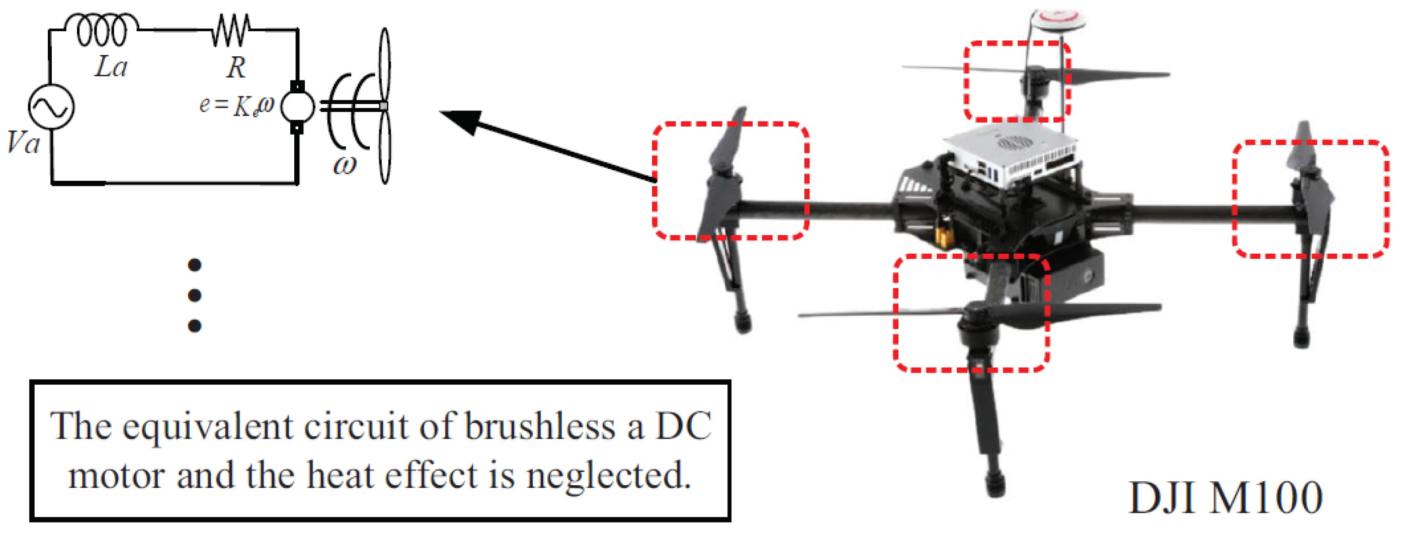
2.3. Energy Model of a Quad-Rotor Aircraft

Quad-rotor control and dynamics have been enormously investigated in the literature [8,9]. A quad-rotor dynamic model can be described by the following equations [9]:

$$\left\{\begin{array}{cc}\ddot{\varphi }=& \dot{\theta }\dot{\psi }\left({\displaystyle \frac{I_y-I_z}{I_x}}\right)-{\displaystyle \frac{I_r}{I_x}}\dot{\theta }\mathrm{\Omega }+{\displaystyle \frac{l}{I_x}}{U}_2\\ \ddot{\theta }=& \dot{\varphi }\dot{\psi }\left({\displaystyle \frac{I_z-I_x}{I_y}}\right)-{\displaystyle \frac{I_I}{I_y}}\dot{\varphi }\mathrm{\Omega }+{\displaystyle \frac{l}{I_y}}{U}_3\\ \ddot{\psi }=& \dot{\varphi }\dot{\psi }\left({\displaystyle \frac{I_x-I_y}{I_z}}\right)+{\displaystyle \frac{1}{I_z}}{U}_4\\ \ddot{z}=& -g+(\mathrm{c}\mathrm{o}\mathrm{s} \varphi \mathrm{c}\mathrm{o}\mathrm{s} \theta ){\displaystyle \frac{1}{m}}{U}_1\\ \ddot{\ddot{x}}=& (\mathrm{c}\mathrm{o}\mathrm{s} \varphi \mathrm{s}\mathrm{i}\mathrm{n} \theta \mathrm{c}\mathrm{o}\mathrm{s} \psi +\mathrm{s}\mathrm{i}\mathrm{n} \theta \mathrm{s}\mathrm{i}\mathrm{n} \psi ){\displaystyle \frac{1}{m}}{U}_1\\ \ddot{y}=& (\mathrm{c}\mathrm{o}\mathrm{s} \varphi \mathrm{s}\mathrm{i}\mathrm{n} \theta \mathrm{c}\mathrm{o}\mathrm{s} \psi -\mathrm{s}\mathrm{i}\mathrm{n} \theta \mathrm{s}\mathrm{i}\mathrm{n} \psi ){\displaystyle \frac{1}{m}}{U}_1\end{array}\right.$$

(3)

$\mathrm{\varnothing }$, $\theta$ and $\psi$ represent the UAV’s roll, pitch, and yaw angles, respectively. x, y, z The variables x, y, and z denote the UAV’s position. $I_x$, $I_y$ and $I_z$ denote the UAV’s moments of inertia about the x, y, and z-axes, respectively. $J_r$ represents the rotor’s moment of inertia, and $m$ is the mass of the UAV. U_i = (i = 1, 2, 3, 4) are intermediate control variables, defined as shown in Equation (4).

The first component in the orientation subsystem accounts for the gyroscopic effect induced by the rigid body’s spatial rotation, while the second term arises from the rotational dynamics of the propulsion assembly.

$$\left\{\begin{array}{cc}{U}_1=& b\left({\mathrm{\Omega }}_1^2+{\mathrm{\Omega }}_2^2+{\mathrm{\Omega }}_3^2+{\mathrm{\Omega }}_4^2\right)\\ U_2=& b\left({\mathrm{\Omega }}_4^2-{\mathrm{\Omega }}_2^2\right)\\ U_3=& b\left({\mathrm{\Omega }}_3^2-{\mathrm{\Omega }}_1^2\right)\\ U_4=& b\left({\mathrm{\Omega }}_2^2+{\mathrm{\Omega }}_4^2-{\mathrm{\Omega }}_1^2-{\mathrm{\Omega }}_3^2\right)\\ \mathrm{\Omega }=& d({\mathrm{\Omega }}_2^2+{\mathrm{\Omega }}_4^2-{\mathrm{\Omega }}_1^2-{\mathrm{\Omega }}_3^2)\end{array}\right.$$

(4)

In Equation (4), ${\mathrm{\Omega }}_i\left(i=\mathrm{1,2},\mathrm{3,4}\right)$ denotes the rotational speed of the i-th motor; $b$ represents the thrust coefficient, and $d$ is the drag coefficient, both determined by the structural characteristics of the UAV.

However, UAVs will unavoidably be affected by wind disturbance in a real environment, which can cause them to experience extra force. As shown in Figure 4, this wind force not only increases the drag on the UAV’s body, but also alters the induced airflow velocity underneath the rotor blades. Consequently, the lift would also differ. Considering that the UAV’s body has a relatively small cross-sectional area, only the effects of wind force on the rotor blades will be taken into account.

The application scenario of this work is as follows: a quad-rotor UAV is used to survey a known region (mainly DEMs) in a 3D environment. Our goal is to use the on-board camera to carry out coverage perception of the whole region with minimal energy consumption while satisfying the observation resolution requirement. Given the above prior conditions, the specific problems to be solved can be formulated as:

$$min\sum _{i=1}^N \sum _{j=1}^K \mathbf{L}(\mathbf{X},\mathbf{U}{)}_{i,j}$$

(5)

where N represents the number of UAVs to be deployed, K is the path number of each UAV, and L denotes the energy cost of a piecewise path (energy consumed by sensors is also included). Since UAVs have six degrees of freedom in translation and rotation, this gives rise to a flexible and varying path even for a fixed starting and ending pose state. As a result, path parameters such as flight time and energy consumption vary significantly under different flight paths. Therefore, it is indispensable to optimize the input control variables in order to minimize the cost function L.

In Figure 5, the problem to evaluate the extrema of L with the given starting and ending points, as well as the corresponding initial and final states, is equivalently expressed in the framework of optimal control. Based on the established control model, a feasible control law is selected to meet predetermined requirements and achieve optimal performance:

$$\underset{u(\mathrm{t})\in \mathrm{\Omega }}{min} J\left(u\right)=\phi \left(\mathit{x}\left(\mathit{t}\right)\right)+{\int }_{t_0}^{t_f} L\left(\mathit{x},\mathit{u}\right)dt$$

(6)

$$\left\{\begin{array}{c} \mathrm{s}.\mathrm{t}. \dot{\mathbf{x}}(t)=f(\mathbf{x},\mathbf{u},t),x\left(t_0\right)={\mathbf{x}}_0\\ \mathbf{\Psi }\left[x\left(t_0\right)\right]=0\end{array}\right.$$

(7)

where $\mathsf{\Psi }(\cdot )$ contains boundary conditions and $\phi (\cdot )$ provides the end term.

3. Optimal Energy Control on Piecewise Path

As a UAV is powered by a battery, its energy is mainly consumed in motor rotation, flight control, and on-board sensors. To achieve accurate estimation of the UAV’s total energy consumption, the three aforementioned energy components are evaluated separately.

3.1. Energy Consumption of Motor Torque

As brushless DC motors have the advantages of large efficiency area, high power and torque density, they have been widely used in UAVs. The equivalent circuit diagram of a brushless DC motor is shown in Figure 6 (for simplicity’s sake, the power loss of a DC motor caused by heat effect is not considered):

Let $e_j(t)$ and $i_j(t)$ be the voltage and current of motor i at time t; then, the energy consumed from 0 to t_f can be described as:

$$E_m={\int }_0^{t_f}{\sum }_{j=1}^4{e}_j(t)i_j(t)dt$$

(8)

Since the current and voltage are mainly decided by motor torque, the above consumed energy can be rewritten as:

$$\begin{array}{c}{E}_m={\int }_0^{t_f}{\displaystyle \sum _{j=1}^4}[c_1+c_2{\omega }_j(t)+c_3{\omega }_j^2(t)+c_4{\omega }_j^3(t)+c_5{\omega }_j^4(t)+\\ c_6{\dot{\omega }}_j(t)+c_7{\dot{\omega }}_j^2(t)+c_8{\omega }_j{\dot{\omega }}_j(t)+c_9{\omega }_j^2{\dot{\omega }}_j(t)]dt\end{array}$$

(9)

where ${\omega }_j(t)$ denotes the angular velocity of the j-th motor, while ${\dot{\omega }}_j(t)$ represents its angular acceleration. And $c_1$ to $c_9$ are parameters decided based on the UAV itself.

3.2. Energy Consumption of Flight Control System

For reliability and real-time precise control, UAVs usually have a flight control board and an on-board computer installed. The former is used to receive control signals from the remote controller and regulate control parameters, while the latter is employed for sensor data processing. Therefore, the energy consumption associated with flight control primarily originates from the onboard computer and the flight control motherboard.

To ensure stable flight, both the onboard computer and the flight control board must operate continuously throughout the mission. Under normal circumstances, the on-board computer does not need to perform large-scale complex operations, and its power consumption can be considered relatively stable. Since the flight control board uses microcontroller units (MCUs) such as single-chip microcontrollers or digital signal processing chips (DSP) as control units, its dynamic power consumption remains below 3 W, which is considered a constant value compared to the on-board computer. Therefore, the energy consumption by the on-board computer and flight control board can be calculated as:

$$E_c={\int }_0^{t_f}(p_c+p_b)$$

(10)

where $p_c$ and $p_b$ indicates the energy consumption from the onboard computer and flight control system, respectively.

3.3. Energy Consumption of Sensors

Sensors carried by UAVs usually include optical cameras, ultrasonic sensors, gyroscopes, magnetometers, pressure gauges and GPS. Since the sensors perform data acquisition according to a certain operating frequency, their energy consumption is determined by their rated power and real-time operating frequency. Assuming that the rated power of a sensor is $p_i$ with a working frequency $f_i$, the energy consumption of the sensor can be formulated as:

$$E_c={\int }_0^{t_f}\sum k_i{p}_i{f}_i$$

(11)

where $k_i$ is the power coefficient decided by the sensor structure.

4. Energy-Optimal Path Planning

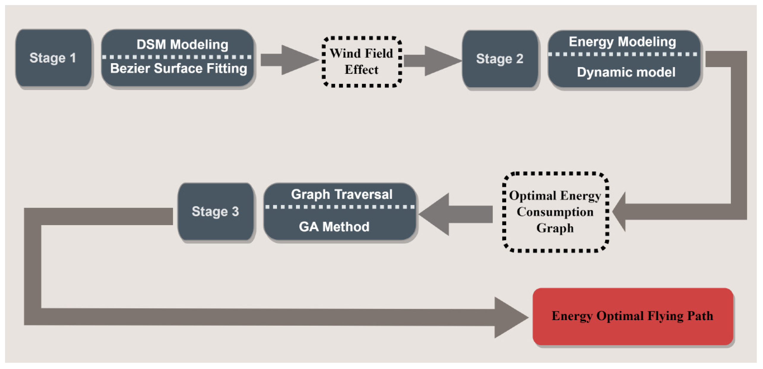
A triple-phase coverage path planning algorithm is introduced as a solution to the previously identified problems. Our method consists of three phases: terrain modeling, optimal flight control on piecewise path, and cost map traversal. In the terrain modeling stage, a Bezier surface is used to characterize the 3D terrain, and the sampling positions of the UAV within the grid area are determined by the predefined observation resolution. Subsequently, the UAV’s dynamic model is employed to derive optimal control parameters that minimize energy consumption along each piecewise segment of the path. Finally, an energy consumption map of the whole area is constructed based on the above results, and an optimized coverage path is figured out. The usual flowchart of this algorithm is described in Figure 7.

Phase 1: Digital surface modeling. To image a terrain surface with a sensor containing uniform resolution, a UAV adapts its position according to the terrain elevation. The nodes at which the UAV captures snapshots are treated as control points of a Bezier surface, from which the analytical parameters of the surface are subsequently derived. Figure 8 shows a closed surface to be observed. Global Mapper software (V14.0) comes with a terrain gridding tool that imports the terrain DEM data and allows grid elements with the longitude, latitude, and altitude information of each grid point to be exported. To determine the UAV’s flight altitude and sampling positions, the normal vectors of each grid area must be calculated, and then a point along the normal vector with a fixed height offset from the grid center is used as the UAV’s observation point.

Phase 2: Optimal power estimation and energy consumption map construction. Combined with the UAV’s dynamic model, the Automatic Control and Dynamic Optimization (ACADO) numerical optimization method is used to optimize energy consumption along the piecewise path as well as the energy consumption map established on this basis. As all sampling points are determined in phase 1, the corresponding starting and ending points, along with the associated UAV flight state information, are used as boundary conditions for the ACADO inputs.

Consequently, the optimal control strategy and the corresponding energy cost for each path segment are computed. To clarify the optimization process implemented in this phase, we present a schematic flowchart in Figure 9, which outlines the core steps of the ACADO-based energy minimization procedure. This includes system modeling, cost function specification, constraint setting, and solver execution, all aligned with the UAV’s dynamic characteristics.

Furthermore, a weighted directed graph G is built to store this consumed energy. It should be noted that the adjacency matrix of this energy consumption map is a non-symmetric matrix, mainly due to factors such as terrain features (such as different relative slope values between two points in space).

Phase 3: Energy-optimal path generation. Given the energy map, the problem of figuring out an energy-optimized coverage path is transformed into a graph traversal problem with minimum cost. For convenience, a weighted directed graph GE = (V, E) is utilized for terrain representation. Specifically, each edge $E$ is associated with the energy cost of the corresponding path segment and $V$ is a vertex set annotated with corresponding elevation values.

Discrete grids can be regarded as destination cities in the TSP model, and the energy cost between paths can be treated as distance between cities. Therefore, the TSP model can be used to solve the traversal problem. Provided the TSP is NP-hard, a GA can be employed for map traversal.

5. Experiments and Performance Evaluation

For performance evaluation, simulation experiments were conducted in the MATLAB@R2022b environment on an Intel(R) Core(TM) i7-9850H CPU with 12 GB memory. Some typical experimental results are shown in Figure 10, Figure 11, Figure 12 and Figure 13, with structural and state parameters used to generate them given in

Table 1. The structural parameters of the DJI M100 UAV.

Kv = 350 rpm/V	nB = 2	ρ = 1.2
KE = 9.5493/Kv	mB = 0.001 kg	m = 2.431 kg
Tf = 4 × 10−2 Nm	r = 0.173 m	£ = 0.319 m
Df = 2 × 10−2 Nms/rad	ε = 0.004 m	Ix = 0.039 kgm2
R = 0.2 Ω	CT = 0.0048	Iy = 0.059 kgm2
Jm = 0.0023 kgm	CQ = 2.3515 × 10−2	Iz = 0.036
ωmax = 1047 rad	CT = 0.0048	mrot = 0.106 kg

and

Table 2. The state settings of the DJI M100 UAV.

$\mathbf{S}\mathbf{t}\mathbf{a}\mathbf{t}\mathbf{e} \mathbf{P}\mathbf{a}\mathbf{r}\mathbf{a}\mathbf{m}\mathbf{s}$	$\mathbf{I}\mathbf{n}\mathbf{i}\mathbf{t}\mathbf{i}\mathbf{a}\mathbf{l} \mathbf{V}\mathbf{a}\mathbf{l}\mathbf{u}\mathbf{e}$	$\mathbf{S}\mathbf{t}\mathbf{a}\mathbf{t}\mathbf{e} \mathbf{P}\mathbf{a}\mathbf{r}\mathbf{a}\mathbf{m}\mathbf{s}$	$\mathbf{T}\mathbf{e}\mathbf{r}\mathbf{m}\mathbf{i}\mathbf{n}\mathbf{a}\mathbf{t}\mathbf{i}\mathbf{o}\mathbf{n} \mathbf{V}\mathbf{a}\mathbf{l}\mathbf{u}\mathbf{e}$
$\mathrm{I}\mathrm{n}\mathrm{i}\mathrm{t} \mathrm{P}\mathrm{o}\mathrm{s}\mathrm{i}\mathrm{t}\mathrm{i}\mathrm{o}\mathrm{n}$	${\left[\begin{array}{ccc}0& 0& 0\end{array}\right]}^T$	$\mathrm{F}\mathrm{i}\mathrm{n}\mathrm{a}\mathrm{l} \mathrm{P}\mathrm{o}\mathrm{s}\mathrm{i}\mathrm{t}\mathrm{i}\mathrm{o}\mathrm{n}$	${\left[\begin{array}{ccc}0& 0& 0\end{array}\right]}^T$
$\mathrm{I}\mathrm{n}\mathrm{i}\mathrm{t} \mathrm{L}\mathrm{i}\mathrm{n}\mathrm{e}\mathrm{a}\mathrm{r} \mathrm{V}\mathrm{e}\mathrm{l}$	${\displaystyle \frac{0 m}{s}}$	$\mathrm{F}\mathrm{i}\mathrm{n}\mathrm{a}\mathrm{l} \mathrm{L}\mathrm{i}\mathrm{n}\mathrm{e}\mathrm{a}\mathrm{r} \mathrm{V}\mathrm{e}\mathrm{l}\mathrm{o}\mathrm{c}\mathrm{i}\mathrm{t}\mathrm{y}$	${\displaystyle \frac{0 m}{s}}$
$\mathrm{I}\mathrm{n}\mathrm{i}\mathrm{t} \mathrm{L}\mathrm{i}\mathrm{n}\mathrm{e}\mathrm{a}\mathrm{r} \mathrm{A}\mathrm{c}\mathrm{c}$	${\displaystyle \frac{0 m}{s^2}}$	$\begin{array}{c}\mathrm{F}\mathrm{i}\mathrm{n}\mathrm{a}\mathrm{l} \mathrm{L}\mathrm{i}\mathrm{n}\mathrm{e}\mathrm{a}\mathrm{r}\\ \mathrm{A}\mathrm{c}\mathrm{c}\mathrm{e}\mathrm{l}\mathrm{e}\mathrm{r}\mathrm{a}\mathrm{t}\mathrm{i}\mathrm{o}\mathrm{n}\end{array}$	${\displaystyle \frac{0 m}{s^2}}$
$\mathrm{I}\mathrm{n}\mathrm{i}\mathrm{t} \mathrm{A}\mathrm{t}\mathrm{t}\mathrm{i}\mathrm{t}\mathrm{u}\mathrm{d}\mathrm{e}$	${\left[\begin{array}{ccc}0& 0& 0\end{array}\right]}^T$	$\mathrm{F}\mathrm{i}\mathrm{n}\mathrm{a}\mathrm{l} \mathrm{A}\mathrm{t}\mathrm{t}\mathrm{i}\mathrm{t}\mathrm{u}\mathrm{d}\mathrm{e}$	${\left[\begin{array}{ccc}0& 0& 0.7854\end{array}\right]}^T$
$\mathrm{I}\mathrm{n}\mathrm{i}\mathrm{t} \mathrm{A}\mathrm{n}\mathrm{g}\mathrm{u}\mathrm{l}\mathrm{a}\mathrm{r} \mathrm{V}\mathrm{e}\mathrm{l}$	$0$	$\begin{array}{c}\mathrm{F}\mathrm{i}\mathrm{n}\mathrm{a}\mathrm{l} \mathrm{A}\mathrm{n}\mathrm{g}\mathrm{u}\mathrm{l}\mathrm{a}\mathrm{r}\\ \mathrm{V}\mathrm{e}\mathrm{l}\mathrm{o}\mathrm{c}\mathrm{i}\mathrm{t}\mathrm{y}\end{array}$	$0$
$\mathrm{I}\mathrm{n}\mathrm{i}\mathrm{t} \mathrm{A}\mathrm{n}\mathrm{g}\mathrm{u}\mathrm{l}\mathrm{a}\mathrm{r} \mathrm{A}\mathrm{c}\mathrm{c}$	${\displaystyle \frac{0 rad}{s^2}}$	$\begin{array}{c}\mathrm{F}\mathrm{i}\mathrm{n}\mathrm{a}\mathrm{l} \mathrm{A}\mathrm{n}\mathrm{g}\mathrm{u}\mathrm{l}\mathrm{a}\mathrm{r}\\ \mathrm{A}\mathrm{c}\mathrm{c}\mathrm{e}\mathrm{l}\mathrm{e}\mathrm{r}\mathrm{a}\mathrm{t}\mathrm{i}\mathrm{o}\mathrm{n}\end{array}$	${\displaystyle \frac{0 rad}{s^2}}$
$\mathrm{I}\mathrm{n}\mathrm{i}\mathrm{t} \mathrm{M}\mathrm{o}\mathrm{t}\mathrm{o}\mathrm{r} \mathrm{S}\mathrm{p}\mathrm{e}\mathrm{e}\mathrm{d}$	$5673 rpm$	$\mathrm{F}\mathrm{i}\mathrm{n}\mathrm{a}\mathrm{l} \mathrm{M}\mathrm{o}\mathrm{t}\mathrm{o}\mathrm{r} \mathrm{S}\mathrm{p}\mathrm{e}\mathrm{e}\mathrm{d}$	$5673 rpm$

.

5.1. UAV Static Power

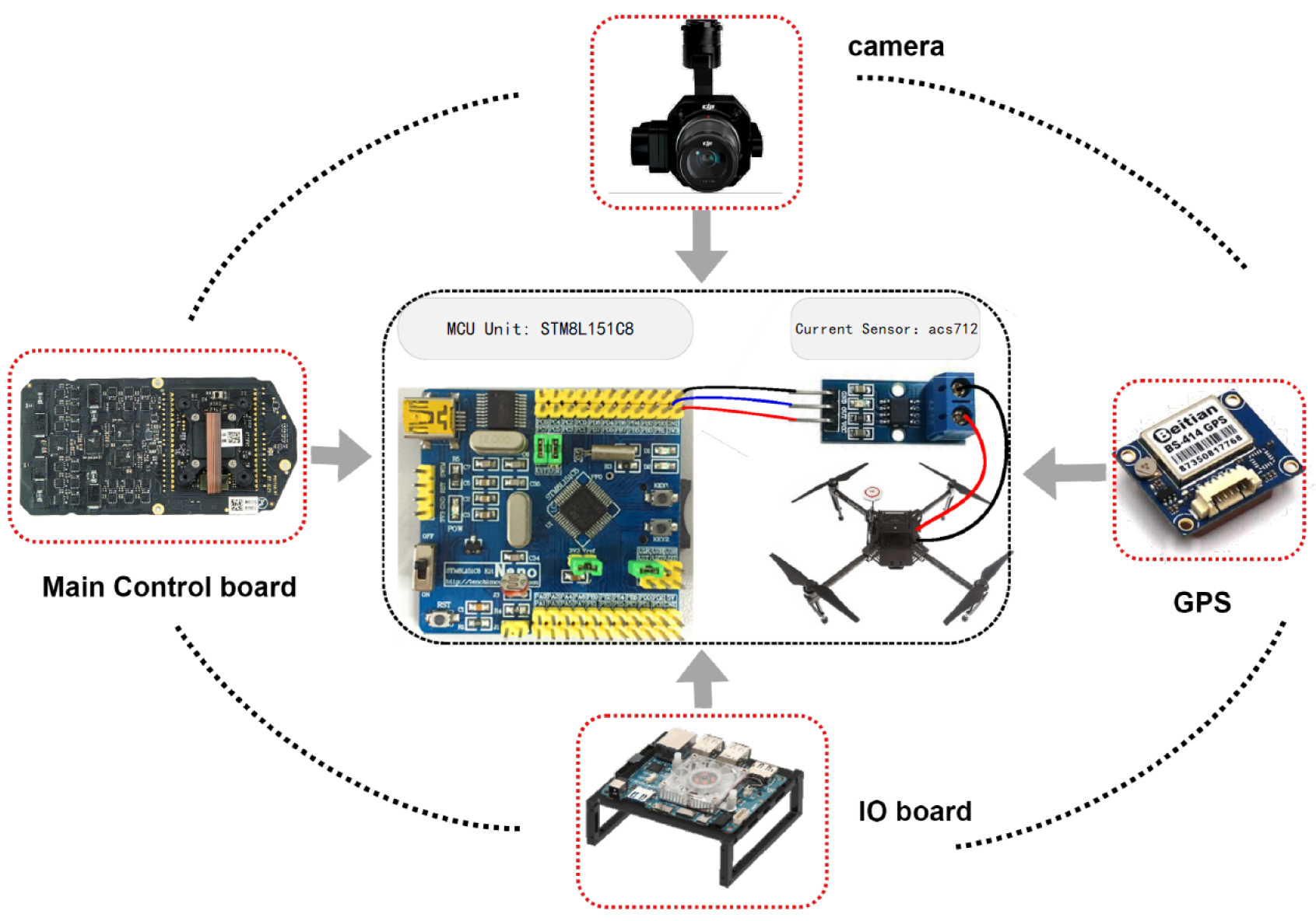
The static power mainly consists of consumption from the flight control board and sensing devices such as the camera and ultrasonic radar. For accurate measurement, we designed a SCM (Single Chip Microcomputer) system (STM8L151C8) equipped with a current sampling module. Therefore, the static power was acquired by setting the UAV to a standby state. Our hardware acquisition system was as follows.

The blue curve denotes the operational current recorded by the designed system, while the red line represents the measurement results after Kalman filtering. During the first few seconds, the UAV ran in an unloaded condition. For observation convenience, the motor power was freely modulated to increase the current measurements. From the above measurement, we can see that the data within the elliptical box retained nearly 0.2 A, which is the static working current of the UAV.

5.2. Coverage Path Planning Results

Accounting for validity, a DJI M100 UAV with a battery capacity of 80.84 Wh was employed for the experiment. The structural parameters were acquired from the operation manual, as follows:

The moment of inertia was obtained based on the CAD model officially provided, and the mechanical parameters of the fuselage as well as the motor-related parameters were acquired through measurements.

Due to feasibility concerns, some variables were constrained during the optimization process based on the theoretical restrictions. Specifically, the angular speed was bounded within 10000 rpm and linear velocity was limited to $-15 \mathrm{m}/\mathrm{s}\le v_x\le 15 \mathrm{m}/\mathrm{s},-15 \mathrm{m}/\mathrm{s}\le v_y\le 15 \mathrm{m}/\mathrm{s},-5 \mathrm{m}/\mathrm{s}\le v_z\le 5 \mathrm{m}/\mathrm{s}$.

In order to verify the effectiveness of our algorithm, simulations were conducted on terrains of three typical scenarios in this section.

Table 3. Terrain geographic information.

$\mathbf{Scenarios}$	$\mathbf{Longitude}$	$\mathbf{Latitude}$	$\mathbf{Size}$
$\mathrm{Scenario} 1$ (Figure 8)	${121}^{\circ }{57}^{\mathrm{\prime }}{18}^{\mathrm{″}} \mathrm{W}-{121}^{\circ }{58}^{\mathrm{\prime }}{37}^{\mathrm{″}} \mathrm{W}$	${46}^{\circ }{43}^{\mathrm{\prime }}{55}^{\mathrm{″}} \mathrm{W}-{46}^{\circ }{44}^{\mathrm{\prime }}{50}^{\mathrm{″}} \mathrm{W}$	$2.861 {\mathrm{k}\mathrm{m}}^2$
$\mathrm{Scenario} 2$ (Figure 12)	${112}^{\circ }{02}^{\mathrm{\prime }}{56}^{\mathrm{″}} \mathrm{W}-{112}^{\circ }{01}^{\mathrm{\prime }}{22}^{\mathrm{″}} \mathrm{W}$	${46}^{\circ }{44}^{\mathrm{\prime }}{13}^{\mathrm{″}} \mathrm{W}-{46}^{\circ }{43}^{\mathrm{\prime }}{24}^{\mathrm{″}} \mathrm{W}$	$3.066 {\mathrm{k}\mathrm{m}}^2$
$\mathrm{Scenario} 3$ (Figure 13)	${122}^{\circ }{12}^{\mathrm{\prime }}{48}^{\mathrm{″}} \mathrm{W}-{122}^{\circ }{09}^{\mathrm{\prime }}{51}^{\mathrm{″}} \mathrm{W}$	${46}^{\circ }{10}^{\mathrm{\prime }}{54}^{\mathrm{″}} \mathrm{W}-{46}^{\circ }{13}^{\mathrm{\prime }}{15}^{\mathrm{″}} \mathrm{W}$	$16.783 {\mathrm{k}\mathrm{m}}^2$

lists the geographic information for the selected three terrains, including longitude and latitude ranges, and their corresponding areas.

To evaluate the performance of our proposed energy-optimized coverage path planning algorithm, we conducted a comparative study against the classical lawnmower-style approach under identical terrain scenarios [30]. The terrain scenarios used in our simulations were uniformly modeled with a grid resolution of approximately 2.861 km²/400, ensuring consistent spatial granularity across all experiments. Each UAV observation footprint was aligned with the normal vector of the corresponding terrain grid, allowing the onboard sensor to maintain perpendicularity to the surface for optimal image resolution. The sampling rate was set to 1/3, meaning that one image was captured for every three grid points, which balanced observation density and energy efficiency in our proposed planning framework.

Table 4. GA parameters for different terrain scenarios.

$\mathbf{Scenarios}$	Bezier Grid Size	Number of Generations	Crossover Probability	Mutation Probability	Population Size
$\mathrm{Scenario} 1$	400	8000	0.9	0.2	7200
$\mathrm{Scenario} 2$	100	8000	0.9	0.2	7200
$\mathrm{Scenario} 3$	1225	8000	0.9	0.2	7200

summarizes the Bezier grid resolution and GA settings used in each simulation scenario, including population size, generation count, and crossover/mutation probabilities. The comparisons include path length and total energy consumption.

Table 5. The coverage path results.

$\mathbf{Scenario}$	$\mathbf{Method}$	$\mathbf{Path} \mathbf{Length} \left(\mathit{m}\right)$	$\mathbf{Energy} \mathbf{Consumption} \left(\mathit{K}\mathit{J}\right)$
$\mathrm{Scenario} 1$	$\mathrm{Proposed} \mathrm{Method}$	${3.225 \times 10}^5$	$9.874 {\times 10}^4$
	$\mathrm{Lawnmower} \mathrm{♯}1$	$3.231 {\times 10}^5$	$1.109{ \times 10}^5$
	$\mathrm{Lawnmower} \mathrm{♯}2$	$3.256{ \times 10}^5$	$1.119{ \times 10}^5$
$\mathrm{Scenario} 2$	$\mathrm{Proposed} \mathrm{Method}$	$2.525{ \times 10}^5$	$5.884{ \times 10}^5$
	$\mathrm{Lawnmower} \mathrm{♯}1$	$1.098{ \times 10}^6$	$3.639{ \times 10}^6$
	$\mathrm{Lawnmower} \mathrm{♯}2$	$4.247{ \times 10}^5$	$1.405{ \times 10}^6$
$\mathrm{Scenario} 3$	$\mathrm{Proposed} \mathrm{Method}$	$1.048{ \times 10}^7$	$3.390{ \times 10}^7$
	$\mathrm{Lawnmower} \mathrm{♯}1$	$2.670{ \times 10}^7$	$8.760{ \times 10}^7$
	$\mathrm{Lawnmower} \mathrm{♯}2$	$1.710{ \times 10}^7$	$5.112{ \times 10}^7$

lists the results for the different coverage path planning methods (including both horizontal and vertical lawnmower paths) for three different terrains. In Table 4, #1 represents a lawnmower path starting from the vertical direction, and #2 represents a lawnmower path starting from the horizontal direction. It can be seen that the proposed coverage path planning algorithm had significant differences in both path length and energy consumption compared to the two classic coverage path planning algorithms. This is because the UAV needed to constantly adjust the flight altitude, which increases energy consumption in the classic coverage path planning algorithms. Even for classic coverage paths with less height adjustment, they still had more energy consumption compared to the proposed algorithm, while the latter could ensure a path length equal to the former. This is because in the classic algorithm: (1) the additional energy consumption caused by the difference in path height was not completely eliminated, and the classic path still followed a zigzag-shaped regular route; (2) the classic path planning method did not quantitatively consider the impact of path length on UAV energy consumption. However, in our method, energy consumption was tightly derived from the immediate dynamics.

Figure 12 and Figure 13 are similar to the scenario depicted in Figure 11, except that the terrain was changed to be rougher. It should be noted that three unmanned aerial vehicles were used to cover the complete area in Scenario 3 considering the battery capacity of a single UAV. To demonstrate the universality and scalability of the algorithm, the takeoff positions of the three unmanned aerial vehicles were randomly assigned. As shown in Table 4, the algorithm designed in this paper also showed superiority in energy consumption and path length compared to classic algorithms.

5.3. Real-World Deployment and Environmental Considerations

The selected terrain scenarios used in this study were representative regions randomly sampled from publicly available DEM datasets. All evaluations were conducted using simulations, incorporating realistic UAV dynamic parameters and authentic elevation data. While physical flight experiments were not performed at this stage, the proposed algorithm was designed with practical deployment in mind. In future work, we plan to transfer the computed coverage paths to real UAV platforms for field trials, validating their performance under operational conditions.

To ensure computational feasibility, the framework adopts a modular, three-stage structure. The most computationally demanding components—such as energy consumption modeling and global path optimization using genetic algorithms—are performed offline. Once the energy-optimal path is generated, it can be uploaded to an onboard flight controller, which executes the trajectory in real time with only light adjustments. This separation allows the system to operate on conventional UAV hardware with limited onboard computing capacity.

Currently, the energy estimation module includes a simplified aerodynamic disturbance model that accounts for a static effect of wind on rotor lift. However, dynamic variations in wind speed and direction are not yet explicitly integrated into the planning framework. In real-world scenarios, such environmental factors may cause fluctuations in energy consumption and impact flight stability. To improve robustness and applicability, future versions of the model will incorporate dynamic wind fields or real-time wind measurement into both the energy model and the control optimization process.

6. Conclusions

In this paper, an energy-optimal coverage path planning algorithm is proposed, which allows UAVs to achieve optimal flight control while satisfying the observation resolution consistency constraint. A DSM was constructed and the energy consumption of a piecewise path was modeled. Under these conditions, a GA-based coverage path planning algorithm was developed to achieve energy minimization. In particular, the effect of wind fields was incorporated into the UAV dynamic model. Numerical results demonstrate that the algorithm is capable of generating an energy-optimal path while simultaneously achieving the constraints of observation quality.