1. Introduction
Control applications compose a significant application domain in the realm of machine learning and neural networks. With classic neural networks, they present a challenge because of the time component, which is not an elemental feature of a classic neural network. They present a moving target—unlike image classification, where the features and the classifications are unchanging, and a simple loss function can be leveraged for training, in a control application, the agent’s actions affect subsequent observations. Simple backpropagation is insufficient as a training technique.
Control applications are a natural fit for neuromorphic processors [
1]. These employ spiking neural networks (SNN’s), in which time is a fundamental element, and memory is co-located with processing. As with most applications for neuromorphic computing, the main challenge is in designing or training the SNN. Nonetheless, SNN’s have been applied successfully to a variety of control problems [
2,
3,
4,
5,
6]. Additionally, solving control problems in a real-world setting with hardware often requires reduced size, weight, and/or power solutions, as well as certain latency requirements. As such, control applications are an interesting application from a hardware perspective as well.
Benchmarks for control applications are inherently more challenging than for classification applications, because the neuromorphic agent must interact with a dynamic system, rather than assign classification labels to a data set. Even a precise mathematical definition of the system may be insufficient to describe a control application, because the definition must be rendered to a computational dynamic system. If the system is real (e.g., a real robotic system), then there are myriad system parameters that are not repeatable from run to run. If the system is simulated, then differing processor architectures and computational environments can also hamper repeatability.
Regardless, benchmarking is essential for a field of study, for without benchmarking, comparison of neuromorphic processors, systems and training methodologies is impossible.
The “cart-pole” problem is a classic control problem [
7,
8]. A wheeled cart is placed on a one-dimensional track. A pole that may “tip” to the left or the right is balanced on the cart. At periodic intervals (typically 1/50 s), information about the cart and the pole is communicated to an agent that may respond with one of two actions: push the cart left or push the cart right. The agent’s objective is to keep the cart within the bounds of the track, and to keep the pole balanced so that its angle to vertical is below a given threshold.
The cart-pole problem is attractive as a benchmark for many reasons. Chief among them are simplicity and availability. Agents receive just four observations: cart position
, cart velocity
, pole angle
, and pole angle velocity (
. At each decision point, they only have two actions: push left and push right. The equations that govern this system are rudimentary and well-documented [
8,
9]. Moreover, a widely available implementation exists as part of the OpenAI Gym project [
10]. It is one of the first applications employed by multiple tutorials on reinforcement learning for classic neural networks (e.g., refs. [
11,
12]), and it is employed as an
ad hoc benchmark in hundreds of papers on reinforcement learning (see
Section 11 below for a sampling).
The benchmark is
ad hoc, because the metrics of success differ from project to project. For example, in one of the earliest applications of neural networks to the problem, Anderson’s goal is 500,000 timesteps without failure [
8]. In Kumar’s tutorial, the goal is to balance the cart for an average of at least 195 timesteps for 100 consecutive episodes [
11]. Ding et al. report that their spiking neural network achieves up to 450 timesteps [
13].
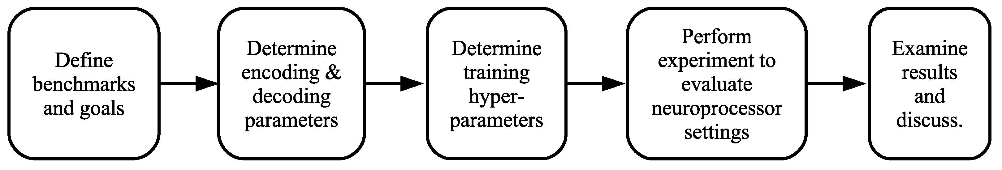
This paper follows the flow diagrammed in
Figure 1. We briefly describe each of the tasks below.
First, we define and present four benchmarks employing the cart-pole application. We present them in detail in
Section 2, but we summarize them here:
Easy: The standard cart-pole problem with a mission time of up to 15,000 timesteps, averaged over 1000 random starting positions (i.e., 1000 different episodes).
Medium: The Easy problem with an additional action: “do-nothing”. The agent must employ “do-nothing” for at least 75 percent of its actions. This is more challenging and also more attractive, as agents focus more on putting the pole into a naturally balanced state, rather than keeping it constantly perturbed.
Hard: The Medium problem with only two observations instead of the standard four–just the position of the cart and the angle of the pole. There are no velocities. Unlike the Medium benchmark, there are no restrictions on the actions chosen. This is a very challenging benchmark, because it encourages the agent to maintain some system state in its “memory”.
Hardest: This is the same as the Hard problem, but the only actions are to push the cart left or right.
For each benchmark, we derive goals for the performance of AI agents. We then perform an experiment to determine the most effective techniques for encoding the cart-pole observations into spikes for SNN agents. The first three benchmarks leverage a “Flip-flop” encoder, where positive and negative values each have their own neurons, and the number of spikes is proportional to the absolute value of the observation. The Hardest benchmark is most successfully solved by an “Argyle” encoder, where each observation results in exactly nine spikes, distributed to two of four input neurons.
We next employ the benchmark to evaluate the effectiveness of eight parameter settings of the RISP neuroprocessor. For the Easy benchmark, the simplest parameter setting of RISP trains effective SNN’s, but as the benchmarks progress in difficulty, richer neuroprocessor parameters are required. The experiment also highlights how one must pay attention to the interplay between the neuroprocessor parameters (in this case, synaptic delay) and the application in order to achieve good training.
Finally, for each benchmark, we present and discuss two example SNN’s, trained in the previous experiment, that achieve the benchmark’s goal. For each, we highlight properties and features of the networks that lead to their success.
Contributions of This Paper
We summarize the contributions of this paper as follows:
We codify four ways in which to employ the cart-pole problem as a benchmark for AI agents, along with target goals for agents to achieve on each benchmark.
We perform an experiment to determine the best way to encode observations into spikes when the AI agent is a neuroprocessor running a spiking neural network.
We perform an experiment to demonstrate how various neuroprocessor parameter settings affect the performance of the neuroprocessor on each of the benchmarks. Along with this, we highlight how to improve the performance by paying attention to how parameter settings interact with the way the observations are encoded.
We highlight features of SNN’s that are useful in neural network design. For example, it is sometimes advantageous to arrange for multiple spikes to arrive at a neuron at different times, so that their effect is additive. Other times, it is advantageous to arrange for the spikes to arrive at the same time, so that their effect is not additive. In such a way, simple SNN constructs may implement, for example, a max() function that helps solve the benchmark.
2. The Cart-Pole Problem
The cart-pole problem is described in multiple places: refs. [
7,
8,
9,
10]. Accordingly, we do not redescribe it here. The following parameter settings are standard with respect to OpenAI gym:
Observations: Cart position , cart velocity , pole angle , pole velocity .
Track extent: −2.4 to 2.4 m. If the cart moves beyond this, it is a failure.
Pole angle: −0.2095 to 0.2095 radians (12 degrees). If the pole falls beyond these angles, it is a failure.
Timestep duration: 1/50 s.
Reward: +1 for each non-failed timestep.
Actions: push left and push right.
The following parameters are non-standard, and are used to make the problem more challenging:
Mission length: 15,000 timesteps, or five simulated minutes. This is much longer than OpenAI’s length of 200 timesteps (4 s) in v0, and 500 timesteps (10 s) in v1.
Starting cart position: between −1.2 and 1.2 on the track. OpenAI’s state is between −0.05 and 0.05.
Starting pole angle: between −0.10475 and 0.10475 radians.
Optional action: do-nothing.
Optional restriction: require 0.75 of actions to be “do-nothing”.
Optional restriction: remove cart velocity and pole velocity observations.
In this paper, we employ the implementation of the cart-pole problem in the TENNLab Exploratory Neuromorphic Computing Framework [
14,
15]. This implementation has been used in multiple evaluations of neuromorphic processors and training algorithms [
4,
5,
16]. We use this as an alternative to the more standard OpenAI implementation because its C++ implementation is much faster than the implementation in OpenAI. Functionally, however, the two implementations are equivalent, as the SNN’s trained using the TENNLab implementation work identically when applied to the OpenAI implementation. The
Easy and
Hardest benchmarks work on OpenAI’s implementation with no modification. The additional parameters for
Medium and
Hard are simple modifications to the OpenAI Python environment. We have verified that the TENNLab-trained networks work identically on OpenAI Gym’s implementation.
3. The Benchmarks and Performance Goals
Below, we give some more description of the benchmarks, plus comments on performance goals for the benchmarks. For these goals, we apply a testing methodology to agents where they must perform the application on 1000 separate instances using 1000 different starting positions/velocities for the cart and pole. The average mission time over a possible time of 15,000 timesteps is reported. The starting positions and velocities used for testing must be different from those that are used for training.
For each benchmark, we give a target fitness, which is a fitness that we have verified to be obtainable, but challenging for spiking neural networks. Selecting a target is a bit of a black art, because training algorithms for regular and spiking neural networks are randomized, and success can be the result of luck. To wit, some of the best neural networks that we have trained have used hyperparameters that typically train poorly, but just happened to “strike gold” in one instance. Thus, our target values are those that should be achieved by a significant fraction of training runs for a set of hyperparameters.
3.1. The Easy Benchmark—Too Easy
With the
Easy benchmark, the agent is given four observations: cart position, cart velocity, pole angle, and angle velocity. The only actions are to push the cart left or right. These are the defaults for both OpenAI Gym and the TENNLab application. After performing many experiments on this benchmark, we agree with Anderson that this version of the problem is too easy [
8]. In particular, Anderson solves the problem mathematically with a four-parameter controller, and concludes that testing random values of controller parameters is as effective as any learning strategy to solve this problem.
However, we believe that it is a good first-step problem for any machine-learning project that involves control applications, and is a necessary stepping stone to more challenging problems. Hence, we set a target fitness for this benchmark of 14,250 timesteps, which is 4 min and 45 s of mission time. Below we show that very simple spiking neural networks exceed this target.
3.2. The Medium Benchmark—More Natural
The Medium benchmark differs from the Easy benchmark in two ways. First, there is a third action in addition to push-left and push-right: do-nothing. Second, the fitness function is adjusted according to how often the do-nothing action is the selected action. The adjustment is defined as follows:
Let the number of timesteps that the agent survives be t.
Let the number of do-nothing actions be d.
Define an “activity threshold”, a, to be a number between 0 and 1.
If , then the fitness is equal to t.
If , then the fitness is equal to .
For example, suppose the agent survives for 500 timesteps, 250 of which are do-nothing actions, and the activity threshold is 0.75. Then the fitness is equal to If the activity threshold is 0.25, then the fitness is 500. As such, a higher activity threshold provides a reward for the do-nothing action.
In the Medium benchmark, we set the activity threshold to 0.75, which promotes more natural and less frantic agents than the Easy benchmark. With the Medium benchmark, the agents only get busy with the cart when the pole is out of balance. Otherwise, they simply let the system be.
Our target fitness for the Medium application is 12,000 timesteps, or 4 min, scaled by the activity factor if necessary.
3.3. The Hard Benchmark—Removing Velocities, but Retaining “Do-Nothing”
With the Hard benchmark, we remove the two observations that report velocities, and instead simply report the position of the cart and the angle of the pole. Without velocities, the agent is encouraged to use its memory of previous observations to determine how to handle the system. We retain the do-nothing action, but remove the activity threshold. The reason is that we have found that agents train more easily with do-nothing as an option.
Our target fitness for this application is 9000 timesteps, or three minutes.
3.4. The Hardest Benchmark—Removing Velocities, and Only Two Actions
With the Hardest benchmark, we remove velocities and restrict the agent’s actions to just push-left and push-right. This benchmark may be achieved using OpenAI gym and simply disallowing the agent to use two of the four observations. In our explorations, this has been the most difficult benchmark for training spiking neural networks.
We define a target fitness for this application as 6000 timesteps, or two minutes. We also note that although we have trained spiking neural networks that well exceed this target, the training process is more difficult than with the other benchmarks.
4. Spiking Neural Networks
According to Roy, spiking neural networks compose the “third generation” of neural networks [
1]. They are the focus of our research. Drawing inspiration from the brain, there has been a large amount of research dedicated to designing
neuroprocessors that operate on spiking neural networks using every kind of hardware imaginable [
17].
We study spiking neural networks as they apply to control applications like the cart-pole problem for two main reasons. First, their temporal operation is a natural fit for the temporal application. Second, their hardware implementations can be very simple, resulting in very low size, weight and power requirements [
18,
19,
20,
21], which are ideal for control agents in the field.
At the core of every neuroprocessor is a collection of integrate-and-fire neurons. Each neuron maintains an action potential whose value may increase or decrease as a result of spikes that arrive from the external environment or from incoming synapses. When the potential meets or exceeds a programmable threshold, the neuron fires, sending spikes along its outgoing synapses.
Each synapse has a programmable delay and weight. When a spike is fired from a synapse’s pre-neuron, then it travels along the synapse to its post-neuron. The duration of this travel is the synapse’s delay. When the spike arrives at the post-neuron, then the synapse’s weight is added to (or subtracted from) the post-neuron’s action potential.
The main feature of spiking neural networks that makes them attractive as computing platforms is their combination of computational expressivity [
22] and low power. Spiking neuroprocessors are fundamentally different from von Neumann computers as there is no central memory or central processing unit that communicates with this memory. Since storage and processing are performed locally, the power demands on the neuroprocessor are reduced.
Various neuroprocessors provide constraints or add features to the description above [
17]. For example, action potentials may have discrete values, upper and lower limits, and may leak their values over time [
23]. They may also have refractory periods where they do not accept spikes for a period of time after they fire [
24]. Synapse delays may be limited to discrete values [
18]. Neuroprocessors may also feature learning rules, where the neuron and synapse properties become modified as a result of how and when they fire [
25]. One popular learning rule is spike time-dependent plasticity (STDP), where a synapse’s weight grows when it causes its post-neuron to fire, and shrinks when it doesn’t [
26].
One of the important usages of benchmarks is to help evaluate the various constraints and features of spiking neural networks. It is currently an open area of research to determine whether the various constraints and features of SNN’s are too limiting, essential or unnecessary. A primary goal of this paper is to aid researchers in using the cart-pole application as one of these benchmarks.
4.1. Spike Encoding
When an application, such as the cart-pole application, presents its observations to a neuroprocessor, it must encode the observations into spikes. Common techniques are rate coding, spike coding, population coding (binning) and temporal coding. Schuman et al. have evaluated multiple encoding techniques on multiple neuromorphic applications and multiple neuroprocessors [
4,
16], and demonstrated conclusively that the encoding algorithm can have a significant impact on the success of a given neuroprocessor on a given application. One of the most affected applications was the cart-pole application [
16]. As such, in this work, we study various spike encoding techniques and include spike encoding recommendations for each of the four benchmarks.
We refer the reader to [
4,
16] for more complete definitions of spike encoding, plus experimental evaluations of encoding techniques. We summarize the encoding algorithms that we explore below:
4.1.1. Values Versus Spikes Versus Time
When applying input to a single neuron, we explore three techniques for conveying information:
Values: A single spike is applied to the input neuron. The weight of the spike is scaled by the value being encoded, potentially after rounding if the neuroprocessor only accepts discrete values.
Spikes: Values are converted into a number of spikes applied to the input neuron periodically. Higher values mean more spikes. The inter-spike duration is the same, regardless of the number of spikes, and each spike has the same weight (typically the maximum weight).
Time: A single spike is applied to the neuron, with maximum weight. The timing of the spike is determined by the value being encoded. One can either have higher values correspond to earlier spikes or to later spikes.
4.1.2. Binning
Binning is a simple form of population coding, where an observation’s value may be converted into spikes that are applied to one of multiple neurons [
27,
28]. These neurons are called “bins”. The domain of the observations’ values is partitioned equally among the bins. For example, the cart’s position, which is a number in the range [−2.4, 2.4], may be converted into spikes that go to two bins—negative values are converted into spikes in the first bin and positive values are converted into spikes in the second bin. Alternatively, if three bins are used, then values in [−2.4, −0.8] become spikes in the first bin, values in [−0.8, 0.8] become spikes in the second bin, and values in [0.8, 2.4] become spikes in the third bin.
Once a bin has been selected, then the conversion of value to spikes is performed as described above in
Section 4.1.1. As above, we refer the reader to [
4,
16] for definitions.
4.1.3. Six Highlighted Spike Encoders
In this paper, we make specific reference to six spike encoders:
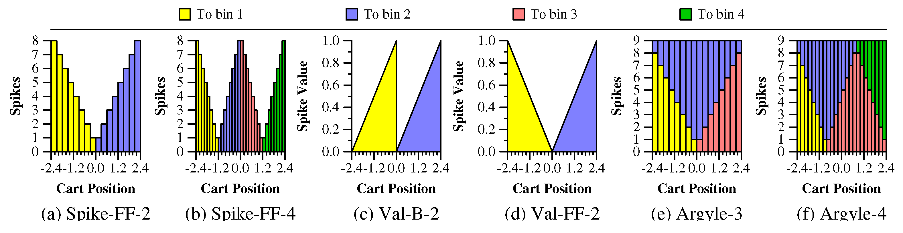
Spike-FF-2: There are two bins, which, for all cart-pole observations, partition the observations into negative values for the first bin and positive values for the second bin. The number of spikes applied to each bin is proportional to the absolute value of the observation, up to a maximum of eight spikes. The “FF” stands for “Flip Flop” [
16]. The spikes all have a maximum charge value, and therefore cause their corresponding neurons to fire.
Figure 2a illustrates how the cart positions are mapped to spikes with Spike-FF-2.
Spike-FF-4: Instead of two bins, there are four bins.
Figure 2b illustrates how the cart positions are mapped to spikes with Spike-FF-4.
Val-B-2: There are two bins, and each value corresponds to a single spike into one of the bins. The spike’s value is proportional to the cart’s position within the interval for the bin, with a maximum value of 1.0.
Figure 2c illustrates how the cart positions are mapped to bins and values with Val-B-2.
Val-FF-2: This is the same as Val-B-2, except the value of the spike to the first bin ranges from 1 to 0 rather than from 0 to 1.
Figure 2d illustrates how the cart positions are mapped to bins and values with Val-FF-2.
Argyle-3: With the Argyle spike encoders, each value puts a total of nine spikes into two bins. With Argyle-3, the first and third bins are identical to the first and second bins of Spike-FF-2. The second bin receives spikes such that the total count of spikes for each value is nine. The name “argyle” comes from the spike encoder documentation within the TENNLab software, version 1d2b769 [
5,
14,
15].
Figure 2e illustrates how the cart positions are mapped to bins and spikes with Argyle-3.
Argyle-4: This continues the “argyle” pattern, but with four spikes instead of three.
Figure 2f illustrates how the cart positions are mapped to bins and spikes with Argyle-4.
4.2. Spike Decoding
As observations must be encoded into spikes that are input to the SNN, output spikes from the SNN must be decoded into actions. For this application, we use one output neuron for each potential action, and then use one of two techniques to decide how to turn spikes on these neurons into actions:
Voting: Here the number of spikes in each neuron is counted, and the one with the most spikes determines the actions. Ties go to the “lower” neuron.
Temporal: The first (or last) neuron to spike is the winner.
Although we test both decoding techniques in our experiments below, the voting decoder emerged as superior in all tests, so we employ that decoder in the remainder of the paper.
4.3. Neuroprocessor
In this work, we use the RISP neuroprocessor [
5]. RISP is a bare-bones neuroprocessor, where neurons simply have programmable thresholds, and synapses have programmable delays and weights. There are some additional features with RISP, such as limiting thresholds and weights to discrete values, and allowing each neuron to be configured to leak all of its potential at each timestep.
Our rationale for focusing on RISP in this work has several components. First, because of its limited nature, RISP may be viewed as a
lingua franca for neuroprocessors—SNN’s developed for RISP may be ported easily to other more complicated neuroprocessors, such as Loihi [
18], Nengo [
29] NEST [
30] or Brian [
31]. Second, because of its simplicity, it is easier to reason about RISP networks and their functionalities than with more complicated neuron models. We do this in
Section 8 below. Finally RISP has open-source support for both CPU simulation and FPGA implementation [
5], making it an ideal neuroprocessor for embedded control applications like the cart-pole application.
5. Training
For the training in this experiment, we use the EONS genetic algorithm [
32] implemented in the TENNLab exploratory neuromorphic computing framework [
14,
15]. We chose this training methodology because of its previous success in training effective, but very small networks for the cart-pole problem [
4,
16]. Other training methodologies, particularly those that rely on backpropagation, result in vastly larger spiking neural networks [
6,
33,
34].
EONs trains unstructured networks, with the synaptic connections being part of the training process. This is what allows the networks to be much smaller than with other training techniques. As such, there are no structural models as there are with, for example, deep learning networks—the structure of the network is part of the training process.
Since independent EONS runs are massively parallel, we employ a large variety of processors for training, including Linux, Macintosh and Raspberry Pi computers of all vintages. Unless otherwise specified, for each test, we run 100 independent optimizations.
6. Spike Encoding and Decoding Experiment
As an initial experiment, for each benchmark, we performed a grid search, similar to the grid search by Schuman et al. [
16], on a variety of encoding and decoding techniques. The number of combinations of techniques was 96. We used the default parameters of RISP (RISP-F, defined below in
Section 7). The goal of this experiment is to determine candidate encoding and decoding techniques for each of the benchmarks, in order to do further explorations. As such, we opted for relatively short optimization runs: In EONS, we used populations of 25 SNN’s, and ran the optimization for 100 epochs. For each test, we performed 75 independent optimizations.
In
Figure 3, we display the testing fitnesses of the best ten encoding techniques for each benchmark. The displays are Tukey plots of the 75 independent runs. On the x-axis, we show the encoder if it is one of the six described in
Section 4.1 above. Otherwise, we omit the label of the encoder.
We have ordered the encoders by their third quartile fitness. The reason is that it is indicative of a “good” optimization for that encoder, that one can expect to achieve or exceed with 10–20 independent optimization runs. We don’t order by the maximum fitness values, because sometimes a run is particularly lucky, and one cannot expect to achieve that fitness except in rare circumstances. Also, note that the Hard and Hardest fitnesses are displayed on different y-axes than Easy and Medium.
For each benchmark, the best two encoders are from the six that we describe in
Section 4.1.3. The
Easy benchmark shows results that are reminiscent of the polebalancing tests in [
16], with a similar encoder (Spike-FF-2) significantly outperforming the others. That encoder also significantly outperforms the others in the
Medium benchmark, which appears to be a much harder problem indeed than the
Easy benchmark.
With the
Hard and
Hardest benchmarks, the various encoders do not differentiate to a great degree in performance. It is interesting that Spike-FF-2 and Argyle-3, whose input spikes are superset of Spike-FF-2 (see
Figure 2a,e), appear in the top ten networks for each of the four benchmarks. Val-B-2 appears in three of the four benchmarks.
From
Figure 3, we conclude that we should focus on Spike-FF-2 as the encoder for the
Easy and
Medium benchmarks. For the others, we must explore further. Accordingly, we performed a second experiment where we only tested the six encoders listed in
Section 4.1, but we extended the optimizations longer. Instead of using populations of 25 SNN’s for 100 epochs, we used populations of 100 networks for 200 epochs. For
Easy and
Medium, we ran 100 independent jobs, and for
Hard and
Hardest, we ran 1000 independent jobs.
We show the results in
Figure 4. A few conclusions stand out from this figure. First, we confirm that Spike-FF-2 is indeed the best encoder of the six on
Easy and
Medium, although in both, Argyle-4 is not far behind. In
Hard, Spike-2-FF and Argyle-3 emerge as the most effective encoders, while in the
Hardest benchmark, there is little discernible difference between Spike-FF-2, Argyle-3, Argyle-4 and Val-B-2.
To explore further, in
Figure 5, we show the fitnesses and encoders for the 25 best networks produced in this experiment. This graph demonstrates that Argyle-4 clearly produces the best networks in
Hardest. In the
Medium test, even though Spike-FF-2 demonstrates the best overall performance, it only produced the 5th best network in the
Medium benchmark. The difference, however, is not quite as pronounced as in the
Hardest benchmark.
As a result of these tests, for the remainder of this work, we use Spike-FF-2 as the spike encoder for Easy, Medium and Hard. For Hardest, we use Argyle-4.
7. Neuroprocessor Experiment—RISP
In this section, we use the four benchmarks to evaluate eight parameter settings of the RISP neuroprocessor. These are the eight “recommended” parameter settings from the open-source RISP simulator [
5]. The settings are detailed in
Table 1. RISP-F+ is the default parameter setting for RISP; however, because it uses floating point for thresholds and weights, it is only supported in CPU simulation. The last six parameter settings are supported by the FPGA version of RISP [
5].
As n gets larger, RISP-n requires more FPGA resources for implementing the neurons and synapses, with RISP-7/RISP-15+ requiring four bits to store weights, thresholds and potentials, and RISP-127/RISP-255+ requiring eight bits. The “plus” variants do not have inhibitory weights, and therefore, may be more limited in what functionalities they can perform. Finally, RISP-1 and RISP-1+ are so limited that their neurons and synapses do not require arithmetic for implementation. As such, one may put larger RISP-1 and RISP-1+ networks onto an FPGA.
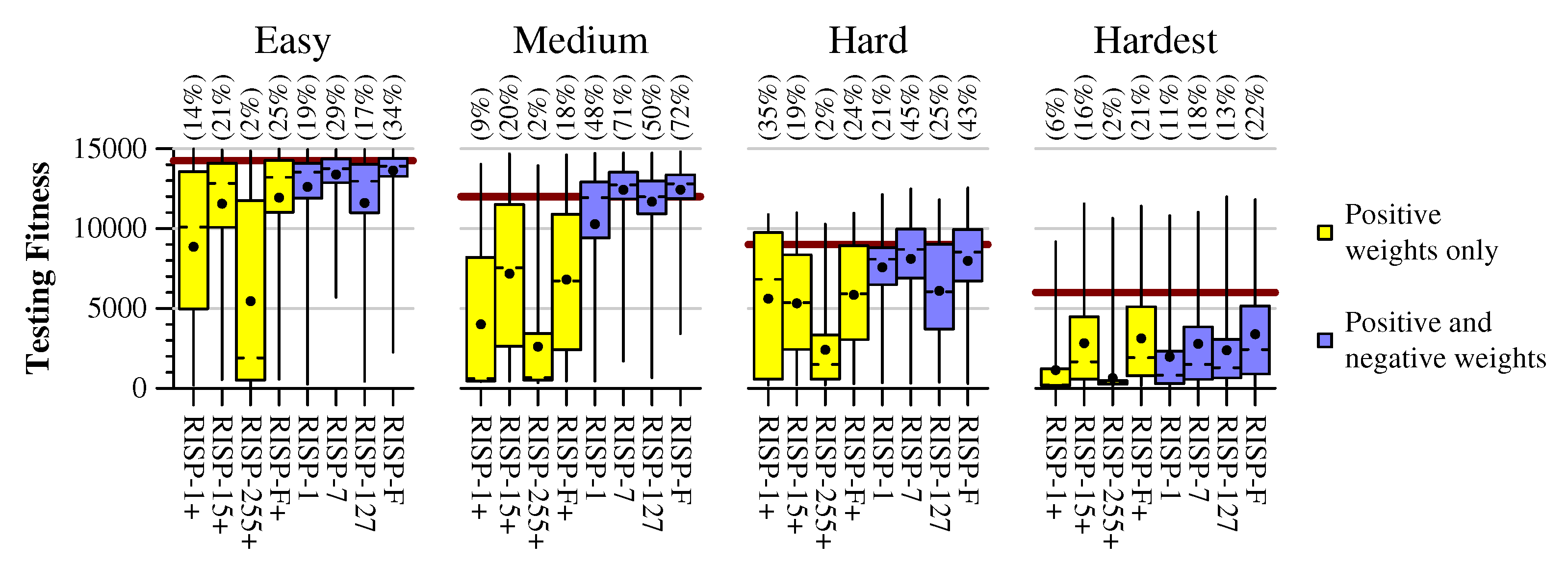
In
Figure 6, we show the results of the eight processor settings with the four benchmarks, using the training parameters shown in
Table 2. The Tukey plots are from 300 independent training runs per parameter setting. The performance goals from
Section 3 are shown on each graph in dark red, and at the top of the graph is the percentage of trained networks that meet or exceed the performance goals.
The benchmarks allow us to draw the following conclusions about the RISP parameter settings. First, the settings that allow negative weights train much better on all four benchmarks. In particular, with the Hard benchmark, the best 3% of the networks all have negative weights. Thus, when selecting a neuroprocessor for these applications, it is more advantageous to use one that employs negative weights.
Second, of the processors with negative weights, the performance, from best to worst, is RISP-F, RISP-7, RISP-127 and RISP-1, with the only non-negligible difference between RISP-7 and RISP-F coming in the
Hardest benchmark. This is significant, because RISP-7, unlike RISP-F, has just 14 synapse weights and neuron potentials, and just 7 neuron thresholds. It has an FPGA implementation [
5] whose small values lead to efficient use of FPGA resources. This is an encouraging result for the effectiveness of RISP-7.
It is also encouraging that the very limited neuroprocessors, RISP-1+ and RISP-1, produce networks that exceed our goals. We present examples in the next section.
The performance of RISP-127 and RISP-255+ is a curiosity relative to the others. The reason is that RISP-127 is a superset of RISP-1 and RISP-7, and RISP-255+ is a superset of RISP-1+ and RISP-15+; yet their performance is worse than their counterparts. We hypothesize that the long delays available in RISP-127 and RISP-255+ penalize their training. Specifically, for each timestep of the cart-pole application, we run the neuroprocessor for 24 timesteps. Therefore, the long delays of RISP-127 (up to 127 neuroprocessor timesteps) and RISP-255+ (up to 255 neuroprocessor timesteps) will cause input spikes during one application timestep to produce output spikes in up to 10 future application timesteps. That is unlikely to be beneficial, or at the very least, makes training difficult.
To test this hypothesis, we reduced the maximum synapse delay in RISP-127 and RISP-255+ to 15, as with the other neuroprocessor settings. The results are in
Figure 7, with the two new data points labeled with “D15”. In these graphs, RISP-127 fits naturally between RISP-7 and RISP-F. Similarly, RISP-255+ fits naturally between RISP-15+ and RISP-F+. This underscores the importance of considering the implications of certain parameter settings with respect to specific applications.
8. Example Networks
In this section, for each benchmark, we present two of the best networks from the previous exploration. For each of these networks, we try to glean some information about which network properties aid in solving the problem, with the hope of figuring out some infomation about “good” network properties, that may be advantageous in designing further good networks.
Each of these networks has been included as an example network in the TENNLab Open Source Neuromorphic Computing Framework, along with of a video of the network controlling the application and instructions on how to employ it in the Gymnasium python environment [
5].
In the networks drawings, the labels
x,
,
and
denote the four input parameters described in
Section 2. Flip-flop encoders use two neurons for each value, so for example,
is used for negative values of
x and
is used for positive values. The neurons labeled
L,
R and − denote the actions “push-left”, “push-right”, and “do-nothing”. Neurons labeled
H are hidden neurons.
8.1. Two Example Easy Networks
In
Figure 8, we show two RISP-1+ networks that were generated in the previous experiments. The left network achieves a testing fitness of 14,970.2 timesteps (4 min, 59.4 s), and the right network achieves a testing fitness of 14,985.0 timesteps (4 min, 59.7 s). Both networks are stunning in their simplicity: Between 7 and 9 synapses each, and no cycles. The
and
inputs are ignored, which is not uncommon for EONS-trained networks. Functionally, when a network ignores one of the two neurons that encode a value, such as the
neuron, it simply treats the lack of spikes on the other neuron (here
) as significant. In the case of the network in
Figure 8a, over the 1000 testing runs, the cart stays in the center 1/8th of the track 94.2% of the time, so even though the
input is ignored, the network does in general center the cart on the track.
The networks are simple enough that each is runnable on nearly all integrate-and-fire neuroprocessors, regardless of whether they are leaky. As such, we verified that the network performs identically on all eight of the RISP settings listed in
Table 1. Moreover, since synapse fires always result in neuron fires, this network is very tolerant of noisy synapses [
35,
36,
37]—the neuron thresholds may be set as low as possible, and the synapse weights as high as possible, to ensure that neurons always fire when synapses fire.
The similarity of the two networks is also striking and worth further examination. In all of these experiments, there are 24 neuroprocessor timesteps per application timestep, and each input value is converted into a number of spikes from zero to eight. Therefore, input spikes potentially arrive every three timesteps. In both networks, the delays on the synapes from
,
and
all have different values when taken modulo 3. Therefore, their spikes always arrive at the
L neuron at different timesteps, and to a first degree of approximation, in both networks, one can calculate the number of spikes arriving at
L as follows:
This calculation is approximate, because there are times when the delays in the synapses mean that the spikes arrive at
L on the next application timestep rather than the current one. In network
Figure 8b for example, if there are more than six spikes from
, three spikes from
, or five spikes from
, then
L receives those spikes in the next application timestep.
This is a very subtle effect, because it happens rarely. Over the course of the 1000 tests, there are spikes that go to the next application timestep in just 0.17% of the timesteps. If the synapse delay from to L is changed from 6 to 9, then the fitness is reduced by 30 timesteps—over half a second.
In both networks, the combination of
,
and
cause the
R neuron to spike, and as with the
L neuron, there are subtleties. In both networks,
and
have synapses whose delays are multiples of three, meaning their spikes align, and therefore are not always summed. For example, suppose that in network
Figure 8b,
spikes once and
spikes twice. The
R neuron receives one spike at time 3 and two at time 6. Because the two arrive simultaneously at time 6,
R only spikes twice instead of three times. This has the effect of implementing a conditional
max operation. Suppose we define
cm(i,j) with the following C code:
int cm(int i, int j)
{
if (i > j) return i;
if (i == 0) return j;
return j+1;
}
Then, we may approximate the number of spikes on
R as:
As with L, there are times when spikes will arrive at R on the next application timestep rather than the current one. Therefore, even though both networks may be reduced to rather simple equations at a high level their actual operation is more subtle.
In
Figure 9, we show the
x observations for a single run of the application on each network. In these graphs, and in subsequent timeline graphs, the starting observations of the system are the same, and all networks run the application successfully for the entire mission time of five minutes. In comparison to subsequent networks, these networks do an excellent job of keeping the cart centered and relatively still. At times, the cart drifts to the right, and then gets corrected (sometimes over-corrected), and goes back to its stable state. It is interesting to note that although the two networks are extremely similar, and although the anomalies in the timeline graphs have very similar shapes, the two networks run quite differently. For example, in the five-minute span, network (a) has three overcorrections, while network (b) has five.
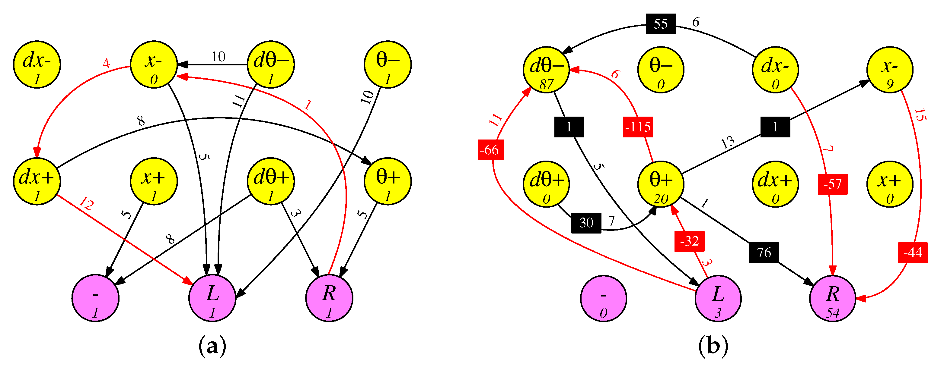
8.2. Two Example Medium Networks
In
Figure 10, we show two networks for the
Medium benchmark. Both well exceed the desired fitness of 12,000 timesteps—the RISP-1 network in
Figure 10a has a testing fitness of 14,698.7 timesteps (4 min, 53.9 s), and the RISP-127 network in
Figure 10a has a testing fitness of 14,820.5 timesteps (4 min, 56.4 s). Both networks have at least 75% of their actions be “do-nothing”, which means that they show considerably less movement than the
Easy benchmark networks. Both networks feature inhibitory as well as excitatory synapses, plus recurrent connections.
Although the networks still feature a small number of synapses (12 and 10), the networks are complex enough that one cannot merely “eyeball” them to draw conclusions about how they work. Instead, we must probe a bit.
Focusing on the network in
Figure 10a, We see that the only times that the “−” neuron spikes is when
or
. Moreover, if
or
, then
L will definitely spike. This raises a curiosity. At a first glance, we would expect for each variable to be positive half of the time and negative half of the time, and for them to be roughly independent. However, were that true, then
and
would both be negative 25% of the time, and in these cases, the “−” neuron does not fire. It is easy to concoct scenarios where
spikes once,
and
spikes more than once. These cannot be “do-nothing” scenarios, so it seems that we cannot have “do-nothing” compose at least 75% of the actions.
The answer must be that the network ensures that the variables are not equally positive and negative, and they are not independent. To confirm, we ran on the testing scenario of 1000 episodes, and see that “do-nothing” is indeed the selected action 82% of the time. This is achieved partially by keeping the cart in the right half of the track—x is positive 97.0% of the time. Similarly, is positive 55.0% of the time, and the combination of either x or being positive occurs 98.4% of the time. Therefore, the network ensures that the “−” neuron is spiking during nearly all application timesteps, skewing the system toward “do-nothing”.
The network in
Figure 10b, on the other hand, never spikes the “−” neuron; yet, “no-action” is the chosen action 81.0% of the time. Therefore, during 81.0% of the timesteps, there are no output neurons that spike. An examination of the network shows that of the 10 synapses, five are positive, with a total weight of 163, while five are negative, with a total weight of −314–clearly the overall nature of this network is to inhibit spiking.
Put another way, the only time that L spikes is when spikes at least three times (9.5% of the time), and the only time that R spikes is when spikes more than and (10.1% of the time). Clearly the network is skewed toward not spiking.
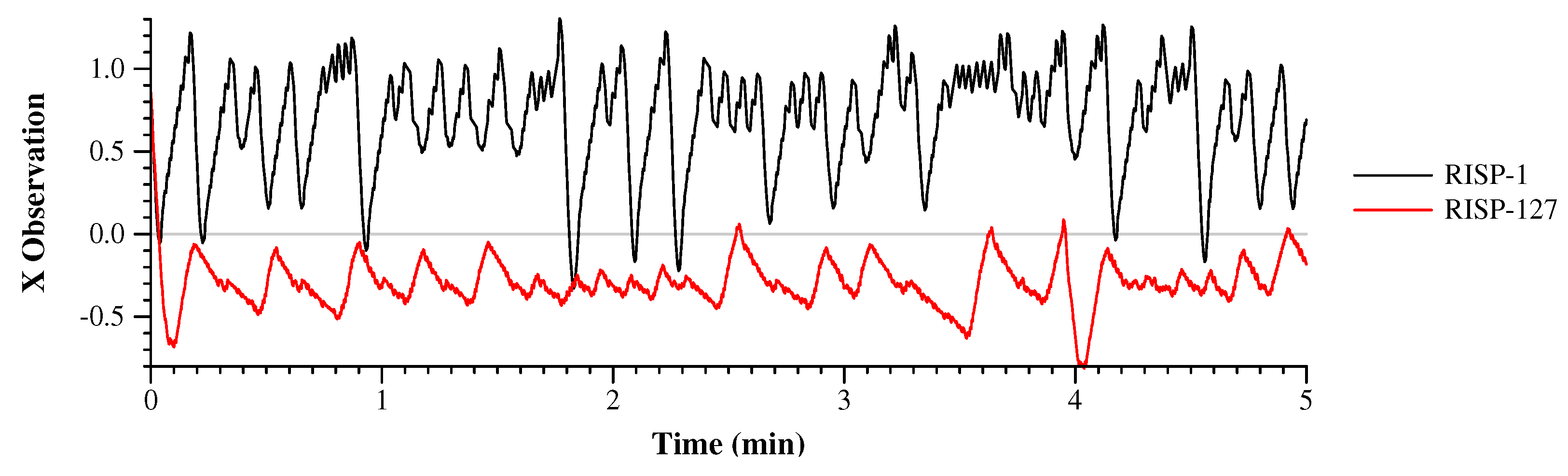
Figure 11 shows the
x observations over time on the same starting parameters as
Figure 9. Since the two lines do not collide, we draw them on the same graph. The RISP-1 network keeps the cart on the right half of the track and the RISP-127 network keeps it on the left half. It is clear from the picture that the RISP-127 network is both less active and less reactive than the RISP-1 network, as the cart travels a lesser distance, and exhibits much less back-and-forth.
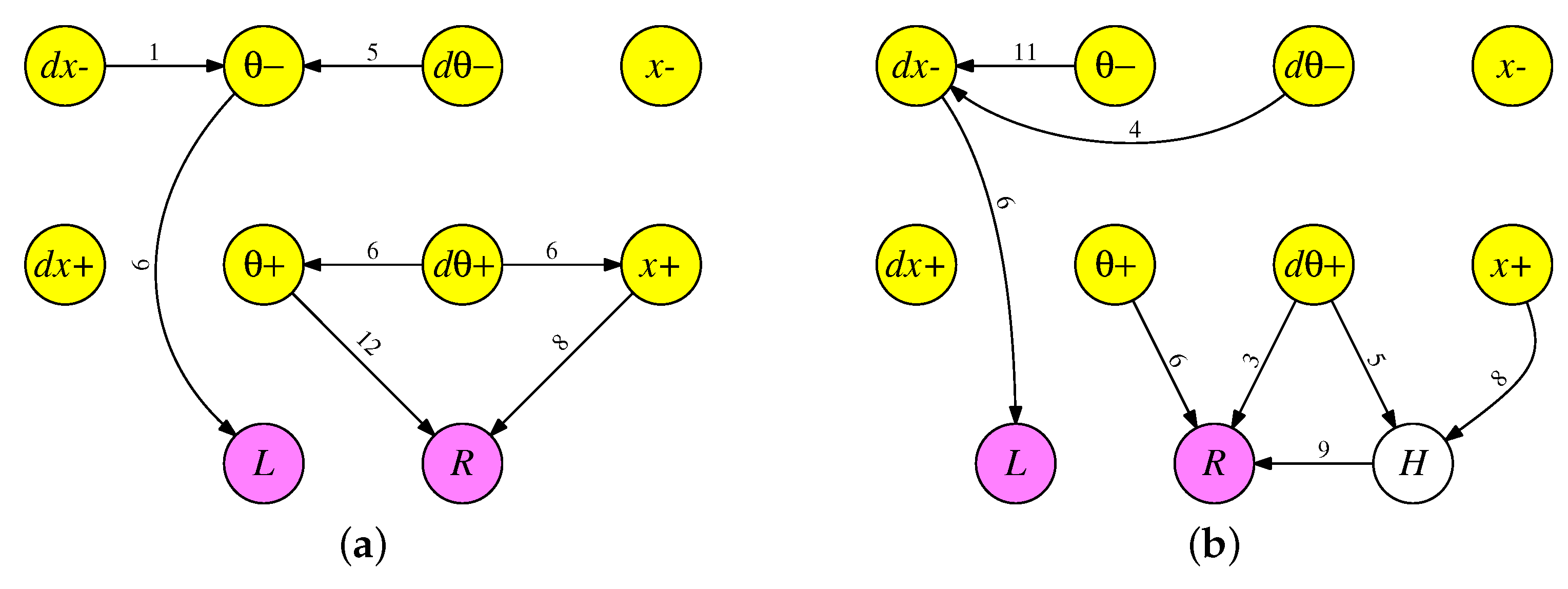
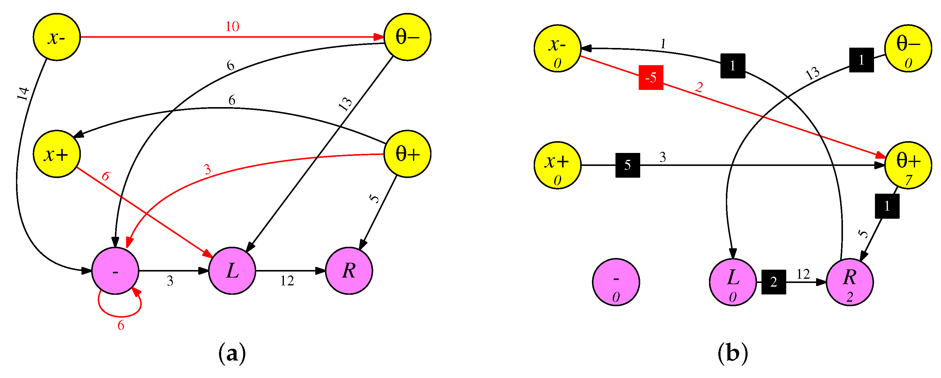
8.3. Two Example Hard Networks
In
Figure 12, we show two networks for the
Hard benchmark. Both exceed the desired fitness of 9000 timesteps—the RISP-1 network in
Figure 12a has a testing fitness of 12,123.8 timesteps (4 min, 2.5 s) and the RISP-7 network in
Figure 12b has a testing fitness of 12,479.3 timesteps (4 min, 9.6 s). Although each network contains a “no-action” action, neither is required to use it.
Both networks are simpler than their
Medium counterparts, featuring fewer neurons and synapses. Focusing on the network in
Figure 10a, 7 of the 10 synapses have delays that are multiples of three, which is reminiscent of the
Easy RISP-1+ networks above, and ensures that some spikes will arrive at neurons simultaneously. For example, neurons
and
have a similar relationship in
Figure 10a as neurons
and
in
Figure 8a. Since all of the neurons have thresholds of zero, when two positively weighted spikes arrive at a neuron simultaneously, the neuron only one spikes once, implementing a functionality like
cm(i,j) in
Section 8.1 above.
The network in
Figure 10b contains only six synapses, and only one of these is inhibitory. One interesting feature of both networks is the path from
to
R, through neuron
L. Consider what happens when
fires. Thirteen timesteps later (in each network), it causes
L to fire, which, 12 timesteps later, causes
R to fire. Thus, whenever neuron
fires during one application timestep, then
L fires either in the same application timestep or the next, and
R always fires in the next application timestep. The effect is one of balance–whenever
L fires,
R fires soon thereafter.
It is interesting that although both networks have a “do-nothing” neuron, neither is required to produce “do-nothing” actions. Regardless, roughly a fifth of each network’s actions are “do-nothing”. We surmise that one reason that the Hard benchmark is easier than the Hardest one is the availability of the action that does nothing.
We show timelines for the two networks in
Figure 13. Both networks oscillate the cart periodically from left to right. The RISP-1 network oscillates roughly every 8 s, keeps the cart on the left side of the track and uses less of the track overall. The RISP-7 network oscillates roughly every 10 s, keeps the cart centered on the track, and travels past
and
on nearly every oscillation.
One feature of the Hard benchmark is that the lack of velocity information encourages the networks to have some notion of memory, from timestep to timestep. The paths from through L to R in each network are a simple examples of memories, where actions from one application timestep are “remembered” and reflected in the next application timestep.
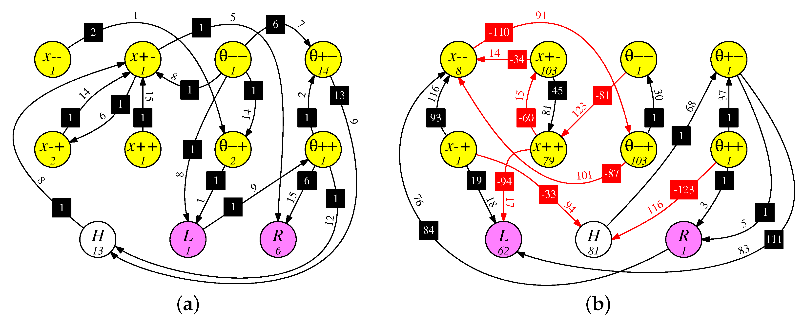
8.4. Two Example Hardest Networks
In
Figure 14, we show two networks for the
Hardest benchmark. As with the other networks, both exceed the desired fitness of 6000 timesteps—the RISP-15+ network in
Figure 14a has a testing fitness of 11,342.9 timesteps (3 min, 46.9 s), and the RISP-127 network in
Figure 14b has a testing fitness of 11,991.6 timesteps (3 min, 59.8 s). Both networks use the Argyle-4 encoder (please see
Figure 2f), where each input causes exactly nine spikes into two of four neurons. As such, the neurons are labeled, for example, from smallest to biggest,
,
,
and
. Each network has a hidden neuron labeled
H.
The RISP-15+ network has 16 synapses, all of which are positive. As with the networks in the previous section, there is a path from L to R (in this case, through ) with a delay of 24, meaning that whenever L fires in one application timestep, then R fires in the next timestep. As will be seen in the timeline graph below, this network has the cart spend the majority of its time (63.1%) on the left side of the track. It should be noted that the longer path lengths in this network provide a memory between application timesteps. For example, the path from to to H to to R has a total delay of 29, which spans application timesteps.
The RISP-127 network was generated during the first set of tests in
Section 7, before we lowered the maximum delays for RISP-127 and RISP-255+ to 15. As such, this network features delays that span many application timesteps. For example, the synapse from
to
has a delay of 123, meaning it spans five application timesteps. This is a longer-term memory than the previous examples, which only span one application timestep. We hypothesize that this may help with the hardest version of the benchmark. To support this hypothesis, we examined the 100 best networks for each benchmark, generated in
Section 7, and counted the number that were RISP-127 with the long delays. The results are in
Table 3, and they do support the hypothesis, although of course they are far from conclusive.
In
Figure 15, we show the
x observations for an example run of each network. As mentioned above, the RISP-15+ network keeps the cart in the left half of the track. Both networks oscillate the cart as in
Hard networks, however in each, there are times when the oscillation is broken, presumably to reach a better steady-state. The RISP-127 network centers the cart and exhibits a much tighter oscillation around
.
In summary, the networks displayed in this section do not exhibit regular structure, which makes it difficult to draw conclusions about them. We have attempted to do so with close examination of the networks combined with measurements of observations, actions and spike counts while they run.
9. Discussion
For a problem to be an effective benchmark, it should first and foremost be widely available, either simple enough for researchers to implement on their own, or having an open-source implementation that is easy to port. The cart-pole application succeeds on this front, particularly with its open-source implementation in OpenAI Gym [
10], which makes it ubiquitously available.
Second, it should provide a variety of challenge levels, from a simple level, such as the Easy setting described here, which serves as a first-level screen and proof-of-concept, to more challenging levels that stress both features of the AI agent and the training methodologies employed. The other three parameter settings provide this challenge.
Last, it should be easy to understand, so that the results have concrete meaning to the observer. The cart-pole problem succeeds in this aspect as well, as visualizations of the application are widely available (as part of OpenAI gym and otherwise), and the fitness metrics of mission time and optionally a prevalence of “do-nothing” actions are quite intuitive.
Even with its simplicity, performing experimentation with the cart-pole problem is not without challenges. Important parameter selections, such as encoding and decoding methodologies, must be made, and as shown in
Section 6, they may impact performance drastically. Similarly, there are an enormous amount of hyperparameters that must be set, which impact both the success of training and how long it takes. Please see the experiments in
Appendix A for examples.
Regardless, the application can be successful in helping to assess the impact of features of a spiking neural network. In
Section 7, we perform such an experiment which demonstrates the impact of inhibitory synapses, range of neuron potentials and synapse weights, and excessive synapse delay, on the effectiveness of training spiking neural networks for the various benchmark levels.
10. Limitations
The experimental work in this paper is inherently limited by the parameter and hyperparameter selections that we made. Although we have attempted to justify these selections with initial experiments and reference to previous work, it remains a fact that there could be other parameter settings that improve results, or that make them more applicable to other systems. Fortunately, our motivation is to demonstrate how the cart-pole problem may be employed to evaluate various neuroprocessors, and as such does not have to perform a complete assessment. It is our intent for this work to pave the way for other researchers to perform additional assessments.
11. Related Work
We have placed related work at the end of the paper, because we feel that it’s best to have context from the results of the paper before explaining the related work. There are too many papers employing the cart-pole problem for machine learning to list, so we focus on a sampling.
As mentioned above, early presentations of this problem by Barto et al. [
7] and Anderson [
8] surmise that the problem is too easy to be an effective machine-learning problem, and that random search for control parameters is often as good of a solution as more complex ones. As mentioned above, we agree that the
Easy benchmark, which is the one on which they focus, is too easy, which is why we focus additionally on harder versions of the problem. Their approach to input encoding is to partition the input space into 162 bins for each of the four parameters, and at each time step, set one of those bins to one, and the other 161 to zero. Their metric is time steps until failure, for which they achieve values exceeding 200,000 on certain trials, while other trials fail very quickly.
In
Table 4, we list 12 sample papers (including this one) and compare them very loosely. The reason for the looseness is that each paper has a different focus, often with a different formulation of execution, success and failure, and with different extensions to the problem. All results pertain to the
Easy benchmark.
We make a final mention to a flamboyant web posting entitled “How to Beat the CartPole Game in 5 Lines—A Simple Solution without Artificial Intelligence”, by Xu [
47]. In this posting, the author proposes the following simple solution to the cart-pole problem that only uses the
and
observations (transposed to C/C++):
char cart_pole(double theta, double dtheta) {
{
if (fabs(theta) < 0.03) return (dtheta < 0) ? ’L’ : ’R’)
return (theta < 0) ? ’L’ : ’R’;
}
When we test this solution on 1000 episodes, it achieves an average fitness of 682.7 timesteps (13.7 s), which succeeds given the objectives of OpenAI Gym, but falls short of the goals of this paper. In contrast, we can build a similar simple agent that sets
L and
R using Equations (
1) and (
2) from
Section 8.1 (including the
cm() function defined there) and compares them:
char cart_pole(double x, double dx, double theta, double dtheta)
{
  double x_p, dx_m, theta_p, theta_m, dtheta_p, dtheta_m, l, r;

  dx_m = (dx < 0) ? -dx : 0;
  theta_m = (theta < 0) ? -theta : 0;
  dtheta_m = (dtheta < 0) ? -dtheta : 0;
  x_p = (x > 0) ? x : 0;
  theta_p = (theta > 0) ? theta : 0;
  dtheta_p = (dtheta > 0) ? dtheta : 0;

  l = ceil(8.0*dx_m/2.0) + ceil(8.0*theta_m/0.209) + ceil(8.0*dtheta_m/2.0);
  r = cm((int) ceil(8.0*dtheta_p/2.0), (int) ceil(8.0*theta_p/0.209))  +
      cm((int) ceil(8.0*dtheta_p/2.0), (int) ceil(8.0*x_p/2.4));

  return (l >= r) ? 'L' : 'R';
}
This agent achieves an average fitness of 14,970.1 on the 1000 testing episodes (0.1 lower than the RISP-1+ network from which it was derived).
12. Conclusions
In this paper, we have examined the well-known Cart-Pole application in detail as it pertains to neuromorphic computing. We have agreed with others that the standard formulation of the problem is not challenging to be employed as a benchmark. Instead, it provides a good starting point for other more challenging benchmarks.
Accordingly, we have defined four parameter settings of the problem, named Easy, Medium, Hard and Hardest. Two of these settings (Easy and Hardest) map directly to the OpenAI Gym environment, and the other two may be employed with some simple modifications. We have also defined target achievements for all four benchmarks.
We have performed extensive experimentation with the Cart-Pole problem on the RISP neuroprocessor. The first experiment determined the best encoding and decoding techniques when rendering the problem on a spike-based neuroprocessor. The second experiment, in
Appendix A, determined recommended hyperparameter settings for using the EONS genetic algorithm [
32] to train spiking neural networks for the four benchmarks. These settings consider both success in fitness and compute time. The third experiment uses results from the first two experiments to determine the effectiveness of eight recommended parameter settings for the RISP neuroprocessor. As anticipated, more complex neuroprocessor features generated more effective networks; however, some features, such as very long maximum synapse delays, needed to be restricted to gain better traction in optimization.
Finally, from the last experiment, we selected eight spiking neural networks that achieve the desired benchmarking goals on the four benchmarks. We explore these networks both quantitatively and qualitatively to reflect on what features they have that enable them to solve the application effectively. The networks for the Easy benchmark are so simple that they do not require integration. Accordingly, they may be applied to any spiking neuroprocessor, even those that feature stochasticity and noise. The RISP-1 network for the Medium benchmark is also exceptionally simple, featuring only excitatory and inhibatory synapses with unit weights. It too may be applied to a variety of neuroprocessors.
The eight networks are included in the TENNLab Open Source Neuromorphic Computing Framework, along with instructions on how to apply them to OpenAI gym [
5]. They may also be executed on the open source RISP FPGA [
5].
With these networks, we have demonstrated that the Cart-Pole problem, in all of its difficulty levels, may be implemented effectively with spiking neural network agents, where the neuroprocessor is quite simple (no leak, refractory periods or learning rules), and the networks are quite small (under 12 neurons and under 20 synapses). The size of these networks, as well as their simplicity, lends them to very efficient neuromorphic hardware implementations.
In demonstrating these small, simple spiking neural networks’ ability to solve various configurations of the Cart-Pole problem, we highlight their ability to operate on applications featuring “state homeostasis”. These types of problems are ubiquitous and are found across domains such as health, aerospace, and many others where low-power solutions are necessary for edge or embedded computing. The networks presented in this work exemplify solutions that are low-SWaP and whose simplicity aids in their explainability.
In future work, we plan to address more control applications, such as those in OpenAI Gym, and those involving UAV control. It is our hope that we may demonstrate, as in this paper, that simple neuroprocessors with relatively small neural networks may be effective agents for these control problems.


