Optimizing Reservoir Separability in Liquid State Machines for Spatio-Temporal Classification in Neuromorphic Hardware

Abstract

In this paper, we propose an optimization approach using Particle Swarm Optimization (PSO) to enhance reservoir separability in Liquid State Machines (LSMs) for spatio-temporal classification in neuromorphic systems. By leveraging PSO, our method fine-tunes reservoir parameters, neuron dynamics, and connectivity patterns, maximizing separability while aligning with the resource constraints typical of neuromorphic hardware. This approach was validated in both software (NEST) and on neuromorphic hardware (SpiNNaker), demonstrating notable results in terms of accuracy and low energy consumption when using SpiNNaker. Specifically, our approach addresses two problems: Frequency Recognition (FR) with five classes and Pattern Recognition (PR) with four, eight, and twelve classes. For instance, in the Mono-objective approach running in NEST, accuracies ranged from 81.09% to 95.52% across the benchmarks under study. The Multi-objective approach outperformed the Mono-objective approach, delivering accuracies ranging from 90.23% to 98.77%, demonstrating its superior scalability for LSM implementations. On the SpiNNaker platform, the mono-objective approach achieved accuracies ranging from 86.20% to 97.70% across the same benchmarks, with the Multi-objective approach further improving accuracies, ranging from 94.42% to 99.52%. These results show that, in addition to slight accuracy improvements, hardware-based implementations offer superior energy efficiency with a lower execution time. For example, SpiNNaker operates at around 1–5 watts per chip, while traditional systems can require 50–100 watts for similar tasks, highlighting the significant energy savings of neuromorphic hardware. These results underscore the scalability and effectiveness of PSO-optimized LSMs on resource-limited neuromorphic platforms, showcasing both improved classification performance and the advantages of energy-efficient processing.

1. Introduction

The rapid evolution of neuromorphic computing has led to a resurgence in the study of computational models inspired by biological neural systems, aiming to process information in a way that is both efficient and capable of handling real-world, dynamic data [1,2,3]. Among these models, Liquid State Machines (LSMs) stand out as a promising framework for processing spatio-temporal data due to their inherent adaptability and efficiency in tasks requiring high temporal precision [4,5]. LSMs leverage a “reservoir” dynamic, using recurrently connected neurons to process information by mapping inputs into high-dimensional representations, which can then be classified or further processed using simpler learning algorithms [6,7]. This property makes LSMs particularly well suited for applications in neuromorphic hardware, where energy efficiency and real-time processing are paramount [8,9,10].

However, one of the fundamental challenges in deploying LSMs for spatio-temporal classification is optimizing reservoir separability, which refers to the reservoir’s capacity to map inputs into distinct, separable states [11,12,13]. High separability enhances the model’s ability to classify complex temporal patterns by creating distinct trajectories for different input signals within the reservoir state space [14]. Achieving optimal separability is crucial for the effectiveness of LSMs, particularly in neuromorphic hardware where constraints on memory and computational resources demand the careful tuning of the network’s parameters and structure [15,16].

In recent years, various approaches have been explored to enhance reservoir separability in LSMs, such as tuning synaptic weights, adjusting connectivity patterns, and optimizing the neuron model’s dynamics [7,13,17,18]. These efforts have yielded promising improvements, yet they often rely on heuristics that may not generalize well to different tasks or hardware implementations. Therefore, the development of systematic optimization strategies for enhancing reservoir separability remains an open problem, with significant implications for the deployment of LSMs in neuromorphic hardware [19]. Additionally, although there have been successful neuromorphic implementations of LSMs, their capability to address several problems using a single liquid and multiple task-related readout models has been scarcely exploited in both software and hardware implementations. For example, in [9], an LSM was implemented on the SpiNNaker board solely to solve the spatio-temporal version of the well-known MNIST benchmark (N-MNIST [20]). This research aims to leverage the capability of LSMs on a neuromorphic platform to address different problems by focusing on improving the separability property of the liquid and simplifying the task-related readout models.

Possible applications of this technology are broad and especially impactful in fields where real-time processing and low power consumption are paramount. In biomedical signal processing, for instance, it holds significant promise for the early detection of conditions such as epilepsy or arrhythmias through the analysis of EEG and ECG signals, which are inherently spatio-temporal in nature. Additionally, this approach can enhance pattern recognition and classification tasks in areas like intelligent surveillance, real-time video analysis, and audio processing, such as robust speech recognition in noisy environments. Since spiking neural networks are particularly adept at handling spatio-temporal data, this technology is well suited for these complex, dynamic signal types. Moreover, brain–computer interfaces (BCIs) could benefit from this technology, enabling more efficient and accurate control of external devices using neural signals, all while minimizing energy consumption.

This paper proposes a novel optimization approach using Particle Swarm Optimization (PSO) to improve the reservoir separability of LSMs specifically for spatio-temporal classification tasks. Our approach demonstrated significant improvements in classification accuracy, with the Mono-objective approach achieving accuracies ranging from 81.09% to 95.52% and the multi-objective approach delivering accuracies ranging from 90.23% to 98.77% for the software implementation. In addition, when implemented on the SpiNNaker neuromorphic system, the Mono-objective approach achieved accuracies ranging from 86.20% to 97.70%, with the multi-objective approach further improving accuracies, ranging from 94.42% to 99.52%. PSO was utilized to systematically evaluate and refine reservoir configurations, enhancing the discriminative power of the network and enabling it to better distinguish between complex input patterns. Our approach leverages recent advances in neural network optimization and is designed with a focus on the constraints and requirements of neuromorphic hardware platforms. Through extensive experimental validation, we demonstrated that PSO-optimized reservoir separability not only enhances classification accuracy but also allows for the more efficient and scalable deployment of LSMs in practical applications. This research contributes to the growing body of work on neuromorphic computing by addressing a core challenge in LSM design and providing a pathway toward more robust and adaptable spatio-temporal classifiers.

The rest of this paper is organized as follows: In Section 2, we provide a detailed description of Liquid State Machines (LSMs) and explain how they are configured within our method, including the spiking neuron model used. In Section 3, we describe the methodology applied to improve reservoir separability based on the classes present in the dataset, along with an overview of the SpiNNaker neuromorphic system and its configuration parameters. Section 4 presents the results obtained from the implementation on SpiNNaker. Finally, conclusions are provided in Section 5.

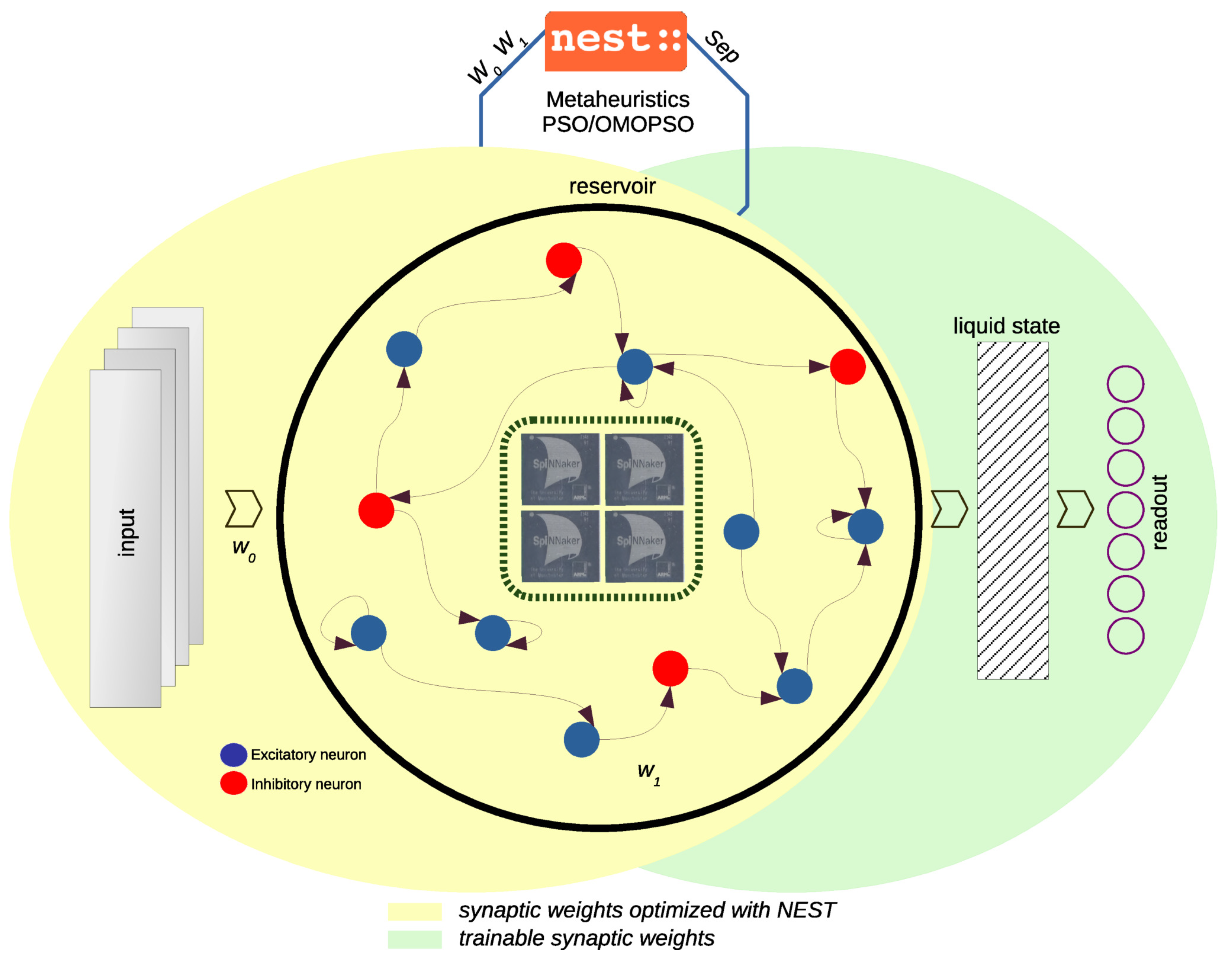
2. Liquid State Machine

A Liquid State Machine (LSM) is a type of recurrent neural network within the family of spiking neural networks and a key model in reservoir computing, inspired by neuroscience [21]. LSMs are designed to process temporal and sequential information efficiently, making them particularly useful for classifying patterns in time series data or data that combine spatial and temporal information.

The structure and functioning of an LSM is as follows:

• The input layer: The input layer receives external signals or sensory data and encodes them into a form suitable for the spiking neurons in the reservoir. This encoding step often transforms a continuous input into discrete events or “spikes” that can be processed by the spiking neurons. In our case, the data are already encoded as spikes, and the number of channels or neurons depends solely on the characteristics of each problem. For a more detailed description of the datasets, see Section 3.3.
• The reservoir (or liquid): This is a recurrent network of randomly connected spiking neurons. The concept of the “reservoir” is that, similarly to how a liquid responds to a stimulus, this component maps input sequences into a high-dimensional representation of its neural states. Each input to the reservoir generates a “splash” of neural activity that varies over time, transforming it into complex spatial and temporal patterns within the reservoir. This process is nonlinear, enabling the capture of temporal relationships in input data, even in complex, high-frequency signals. In our case, the reservoir consisted of 64 randomly connected neurons, using the Integrate-and-Fire neuron model with exponential synaptic currents, denoted as IF_curr_exp, as defined in Equation (1). In this setup, 80% of the neurons were excitatory (E) and 20% were inhibitory. Here, ${\tau }_m$ represents the membrane’s time constant, $V_m$ is the membrane potential, $C_m$ is the membrane’s capacitance, $V_{rest}$ is the resting potential, and $I_{syn}$ is the total synaptic current, which is the sum of both the excitatory and inhibitory currents.

  $${\displaystyle \frac{d{V}_m}{dt}}=-{\displaystyle \frac{(V_m-V_{rest})}{{\tau }_m}}+{\displaystyle \frac{I_{syn}}{C_m}}$$

  (1)
  The neuron parameters implemented in NEST and on SpiNNaker through PyNN are given in

  Table 1. Neuron parameters.

  Parameters	Description	Value
  $C_m$	Membrane’s capacitance	0.05 nF
  ${\tau }_m$	Membrane’s time constant	1.0 ms
  $V_{th}$	Threshold	0.8 mV
  $V_{reset}$	Reset potential	−0.06 mV
  $V_{rest}$	Resting membrane potential	−0.06 mV

  .
  To define connectivity within the reservoir, we arranged the 64 neurons in a $4\times 4\times 4$ grid, where each neuron connected to another based on a specified probability. The synaptic connectivity probability, proposed by [22], is defined in Equation (2).

  $$p(a,b)=C\times e^{-{\left({\displaystyle \frac{D(a,b)}{\lambda }}\right)}^2}$$

  (2)

  where C represents the probability associated with the synaptic connection type (presynaptic–postsynaptic) among neurons; it was set at 0.3 for excitatory–excitatory (EE), 0.2 for excitatory–inhibitory (EI), 0.4 for inhibitory–excitatory (IE), and 0.1 for inhibitory–inhibitory (II) connections. D denotes the Euclidean distance between two neurons, while $\lambda$ indicates the average number of connections and distances among neurons, set to a value of 2, thereby reducing synaptic connectivity within the reservoir. Synaptic weights in both the reservoir and the input layer were generated from a normal distribution with a mean of $2\times {10}^{-2}$ and a standard deviation of $4\times {10}^{-2}$, ensuring that they remained representable at lower precisions. Connectivity between the input layer and the reservoir was defined with a probability of 0.3. Additionally, each neuron in the reservoir was subject to noise, drawn from a normal distribution with a standard deviation of $5\times {10}^{-4}$ nA, and a synaptic delay of 1.0 was incorporated.
• Readout (or output layer): Unlike traditional recurrent neural networks, training in LSMs is only performed on the output layer. In our approach, this output layer was composed of perceptron neurons, which were trained using an Adaptive Moment Estimation (Adam) optimizer with the Softmax activation function using default parameters over 1000 epochs.

3. Materials and Methods

Our methodology, illustrated in Figure 1, was designed to enhance the performance of the liquid state in Liquid State Machines (LSMs) by increasing its separability [23], which is crucial for improving classification accuracy in multi-class data scenarios [24]. To achieve this, we applied Particle Swarm Optimization (PSO), leveraging both single-objective and multi-objective optimization approaches to fine-tune the liquid’s separability properties. PSO was particularly well suited for this task due to its effectiveness in optimizing non-differentiable functions, which was essential given the spiking nature of neurons in LSMs. Traditional gradient-based optimization methods were not applicable in this context because the spiking behavior of neurons introduces discontinuities that prevent the calculation of gradients [25]. By using PSO, we could circumvent these limitations and systematically improve the liquid’s ability to differentiate between different input patterns. The PSO process involved initializing a swarm of candidate solutions, each representing a potential configuration of the liquid’s parameters. These candidates were evaluated based on their performance in enhancing separability, and they iteratively adjusted their positions in the parameter space by considering their own best performance and the best performances observed by the swarm. This iterative process continued until a satisfactory level of separability was achieved. In our approach, this optimization was performed offline, allowing for a thorough search of the parameter space without the constraints of real-time processing. Once the optimal parameters were determined, the enhanced liquid state was then deployed on a neuromorphic platform, such as SpiNNaker, which is capable of emulating the spiking neuron dynamics efficiently.

3.1. Separability Metric

The reservoir’s performance was evaluated using the separability metric introduced in [14]. This metric measured how effectively the reservoir transformed inputs into distinct, separable states, thereby enhancing the readout layer’s ability to classify these states accurately. The separability metric is defined as the ratio of the inter-class distance $c_d$ to the intra-class variance $c_v$, with 1 added to the denominator to prevent division by zero, as shown in Equation (3). This evaluation was applied to the set of state vectors $\mathit{O}$, determined by the reservoir’s firing rate over the final 50 ms of the simulation.

$$Se{p}_M\left(\mathit{O}\left(t\right)\right)={\displaystyle \frac{c_d\left(t\right)}{c_v\left(t\right)+1}}$$

(3)

The inter-class distance, $c_d$, is defined as the average distance between the centers of mass for each pair of classes, as expressed in Equation (4).

$$c_d\left(t\right)=\sum _{l=1}^n\sum _{m=1}^n{\displaystyle \frac{\left|\right|\mu \left({\mathit{O}}_l\left(t\right)\right)-\mu \left({\mathit{O}}_m\left(t\right)\right){\left|\right|}^2}{n^2}}$$

(4)

where $\mu \left({\mathit{O}}_l\left(t\right)\right)$ and $\mu \left({\mathit{O}}_m\left(t\right)\right)$ represent the centers of mass for the classes l and m, respectively. The total number of classes in the problem is denoted by n. The center of mass for the l-th class is given by the following equation:

$$\mu \left({\mathit{O}}_l\left(t\right)\right)={\displaystyle \frac{{\sum }_{o_m\in {\mathit{O}}_l\left(t\right)}{o}_m}{|{\mathit{O}}_l\left(t\right)|}}$$

(5)

with $|{\mathit{O}}_l\left(t\right)|$ representing the quantity of state vectors that correspond to the l-th class.

On the other hand, the intra-class variance $c_v$ is defined as the average variance of each cluster of state vectors, and it is calculated as follows:

$$c_v\left(t\right)={\displaystyle \frac{1}{n}}\sum _{l=1}^n\rho \left({\mathit{O}}_l\left(t\right)\right)$$

(6)

In Equation (6), the term $\rho \left({\mathit{O}}_l\left(t\right)\right)$ indicates the mean variance of the state vectors belonging to the class l, as outlined in Equation (7).

$$\rho \left({\mathit{O}}_l\left(t\right)\right)={\displaystyle \frac{{\sum }_{o_m\in {\mathit{O}}_l\left(t\right)}\left|\right|\mu \left({\mathit{O}}_l\left(t\right)\right)-o_m{\left|\right|}^2}{|{\mathit{O}}_l\left(t\right)|}}$$

(7)

3.2. Optimization Methods

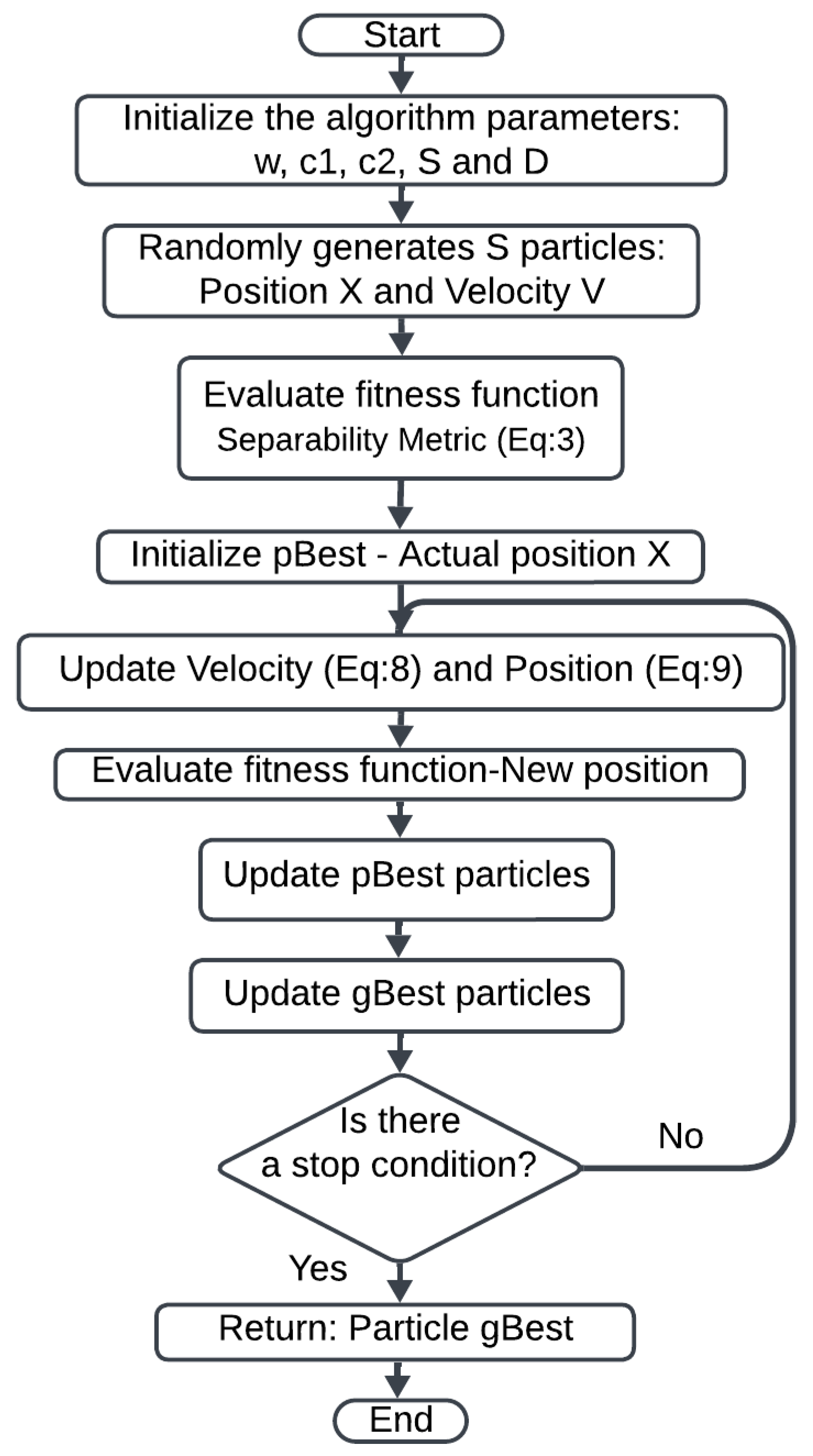
3.2.1. Particle Swarm Optimization

Particle Swarm Optimization (PSO) [26,27] is an optimization algorithm inspired by the collective behavior of swarm individuals observed in nature. A swarm consists of a group of elements known as particles, which are responsible for exploring and exploiting the d-dimensional search space in a given optimization problem to find the best solution based on the combined experience of all particles. For this research, the value of d could not be explicitly defined because it depended on the characteristics of the liquid. Since the liquids were initially created randomly based on the connectivity between the input layer and the liquid, as well as the internal neuron connectivity, the value of d varied accordingly. The search process was guided primarily by two key attributes of each particle: its velocity V and position X. Velocity represents the direction and speed of movement from the current position to the next position within the search space during each iteration. Position corresponds to the particle’s current location in the search space.

In each iteration, k, the particles required an update, which involved obtaining two key values:

• $p_{Best}$ refers to the best position of each particle.
• $g_{Best}$ represents the best position achieved by the entire swarm of particles.

Using $p_{Best}$ and $g_{Best}$, PSO updated the velocity through Equation (8) and the position through Equation (9).

$$V_d^i(k+1)=\omega V_d^i\left(k\right)+c_1{r}_1\left(p_{Bes{t}_d^i}-X_d^i\left(k\right)\right)+c_2{r}_2\left(g_{Bes{t}_d^i}-X_d^i\left(k\right)\right)$$

(8)

$$X_d^i(k+1)=X_d^i\left(k\right)+V_d^i(k+1)$$

(9)

where we have the following:

• $V_d^i$ is the d-th value of the i-th particle’s velocity.
• $\omega$ is the inertia weight.
• $c_1,c_2$ are the cognitive and social acceleration coefficients.
• $r_1,r_2$ are two uniform random values generated within the $\left[0,1\right]$ interval.
• $p_{Bes{t}_d^i}$ is the d-th value of the personal best position.
• $g_{Bes{t}_d^i}$ is the d-th value of the global best position.
• $X_d^i$ is the d-th value of the i-th particle’s position.

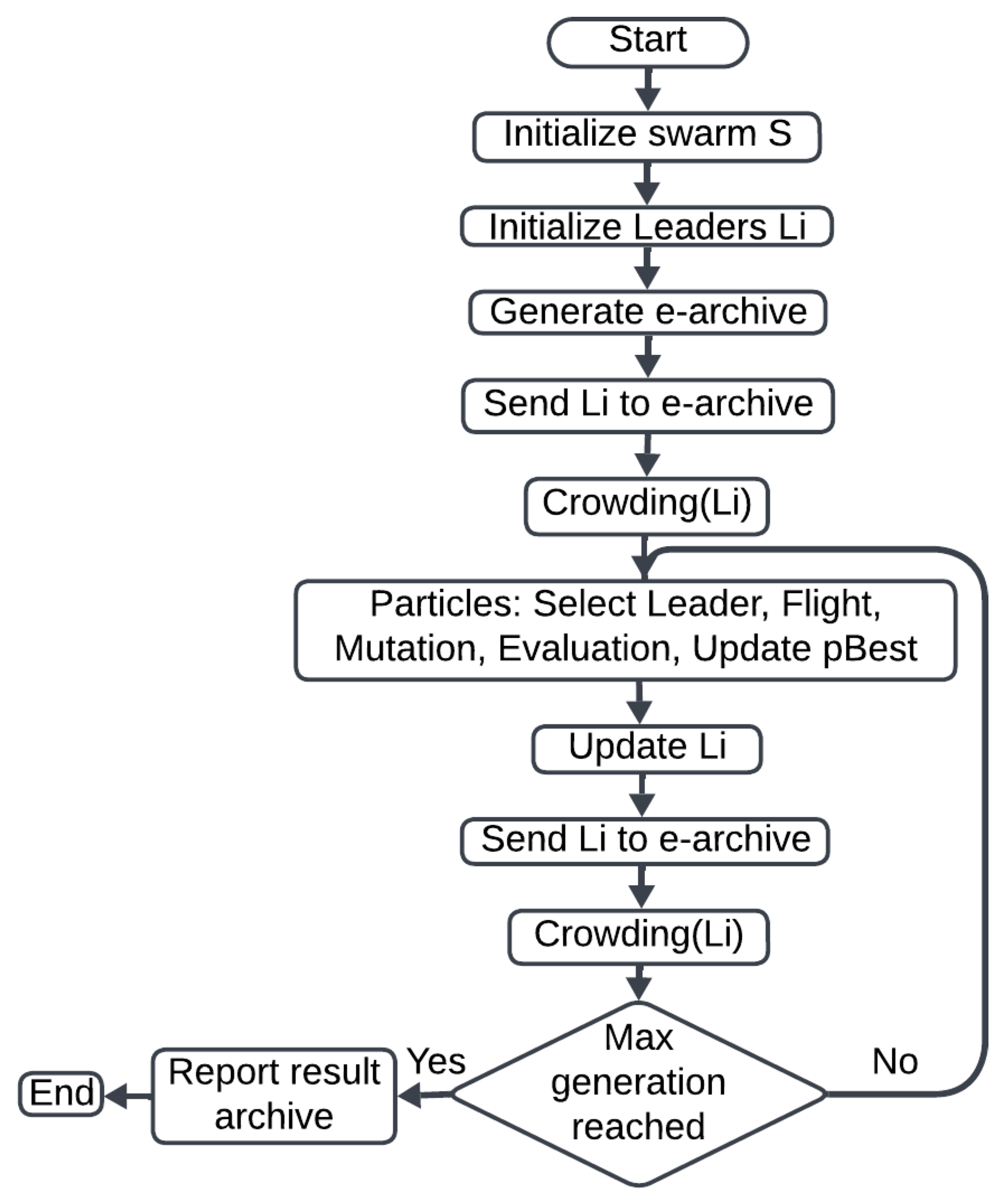
Figure 2 presents a diagram illustrating the methodology for implementing PSO. We started by initializing the parameters $\omega ,c_1,c_2$ as previously described, along with S, the number of particles, and D, the problem dimensionality. A swarm of S particles was generated, each with an initial position, X, and velocity, V. Each particle was then evaluated based on the fitness function (separability level from Equation (3)) in its current position, X, with this initial position serving as the initial $p_{Best}$ value.

As long as no stopping condition was met, both the velocity and position of each particle were updated, and the fitness function was evaluated. We then updated $p_{Best}$ and $g_{Best}$ accordingly. Ultimately, the particle with the best $g_{Best}$ was obtained as the solution.

3.2.2. OMOPSO

The Original Multi-Objective PSO (OMOPSO) [28] is an algorithm proposed to solve multi-objective optimization problems. It is a variant of Multi-Objective Particle Swarm Optimization (MOPSO) [29], an extension of the PSO algorithm designed specifically for multi-objective optimization. When addressing complex problems with conflicting objectives, it becomes essential to generate a set of non-dominated solutions. These optimal solutions offer a balanced representation for multi-objective problems and are organized along the Pareto front, enabling the consideration of multiple optimal solutions to a given problem.

Figure 3 illustrates the methodology for implementing OMOPSO. The process begins by initializing a swarm with S particles and selecting an initial set of leaders. An external archive (e-archive) is generated to store these initial leaders. Crowding is applied to control the distribution of particles within the search space. The update for each particle is then based on the following steps:

• Select Leader: the selection of a leader from the e-archive to guide the particle’s movement.
• Flight: updating the particle’s velocity and position based on the previously selected leader.
• Mutation: the implementation of mutation to introduce variability.
• Evaluation: the particle’s updated position is evaluated based on the fitness function.
• Update $p_{Best}$: updating $p_{Best}$ if a better performance is achieved during the evaluation.

Once the update process for each particle is complete, the leaders, $L_i$, are updated by transferring the non-dominated solutions to the e-archive and applying crowding again. If no stopping condition, such as the maximum number of generations, is met, the particles are updated once more. Otherwise, the e-archive containing the solutions is obtained.

3.3. Dataset

Our approach utilized four datasets, initially proposed in [14]: Frequency Recognition with 5 classes (FR5), Pattern Recognition with 4 classes (PR4), Pattern Recognition with 8 classes (PR8), and Pattern Recognition with 12 classes (PR12). Each dataset consisted of 400 instances per class for training and 100 instances per class for testing, totaling 2000 and 500, 1600 and 400, 3200 and 800, and 4800 and 1200 instances for the FR5, PR4, PR8, and PR12 training and test sets, respectively. In the single-objective phase, the PR4, PR8, and PR12 datasets used 8 neurons each, while FR5 employed 4 neurons. However, for the multi-task phase, the FR5 dataset was modified to ensure consistent dimensionality in synaptic connectivity across all tasks, which required each problem to have the same number of channels or neurons. Therefore, 4 non-spiking channels were added to FR5 in this phase. Figure 4 shows a sample from each dataset.

3.4. Offline Training with the NEST Framework

For the experiments, the NEST (Neural Simulation Tool) framework [30] and PyNN [31] were used. NEST was employed to simulate spiking neural networks, while PyNN served as an interface for implementing experiments both in NEST and on SpiNNaker. NEST is a spiking neural network simulator that captures the dynamics of neuronal action potentials, efficiently representing the heterogeneity of biological neural networks. PyNN is an interface for spiking neural networks that facilitates the use of different simulators without requiring significant modifications between them.

A total of 33 experiments were conducted for both the single-objective and multi-objective implementations, using only 3 randomly selected samples per class with replacement. These were simulated with PyNN and NEST prior to implementation on SpiNNaker. In the single-objective phase, the total number of experiments were conducted independently for each dataset. In the multi-objective phase, only 33 experiments were performed, including all the datasets. In each experiment, a total population of 25 individuals was used. This value was selected because it falls within the range suggested by the literature, which recommends using between 20 and 30 particles [32,33]. Additionally, we conducted experiments with a population of 50 particles [34,35], but no significant improvement in performance was observed. Thus, the population size of 25 was deemed optimal for the experiments, balancing performance and computational efficiency. The initial individual was defined by the synaptic weights obtained before the optimization process. Then, 24 additional individuals were generated by introducing Gaussian noise, thus completing the total population. One limitation of implementing SpiNNaker with PyNN is that synaptic weights are stored as 16-bit integers. Since the optimization process involved fine-tuning the model in each experiment, the synaptic weights were treated as fixed-point values with 16-bit precision. This approach allowed for more representative behavior on SpiNNaker compared to what was experienced in NEST. In each experiment, the goal was to improve the LSM’s performance by optimizing the synaptic weights of the input layer and reservoir through the separability metric, evaluated with the state vectors. The state vectors in this study were obtained from the firing rate of each neuron during the last 50 ms of a 100 ms simulation.

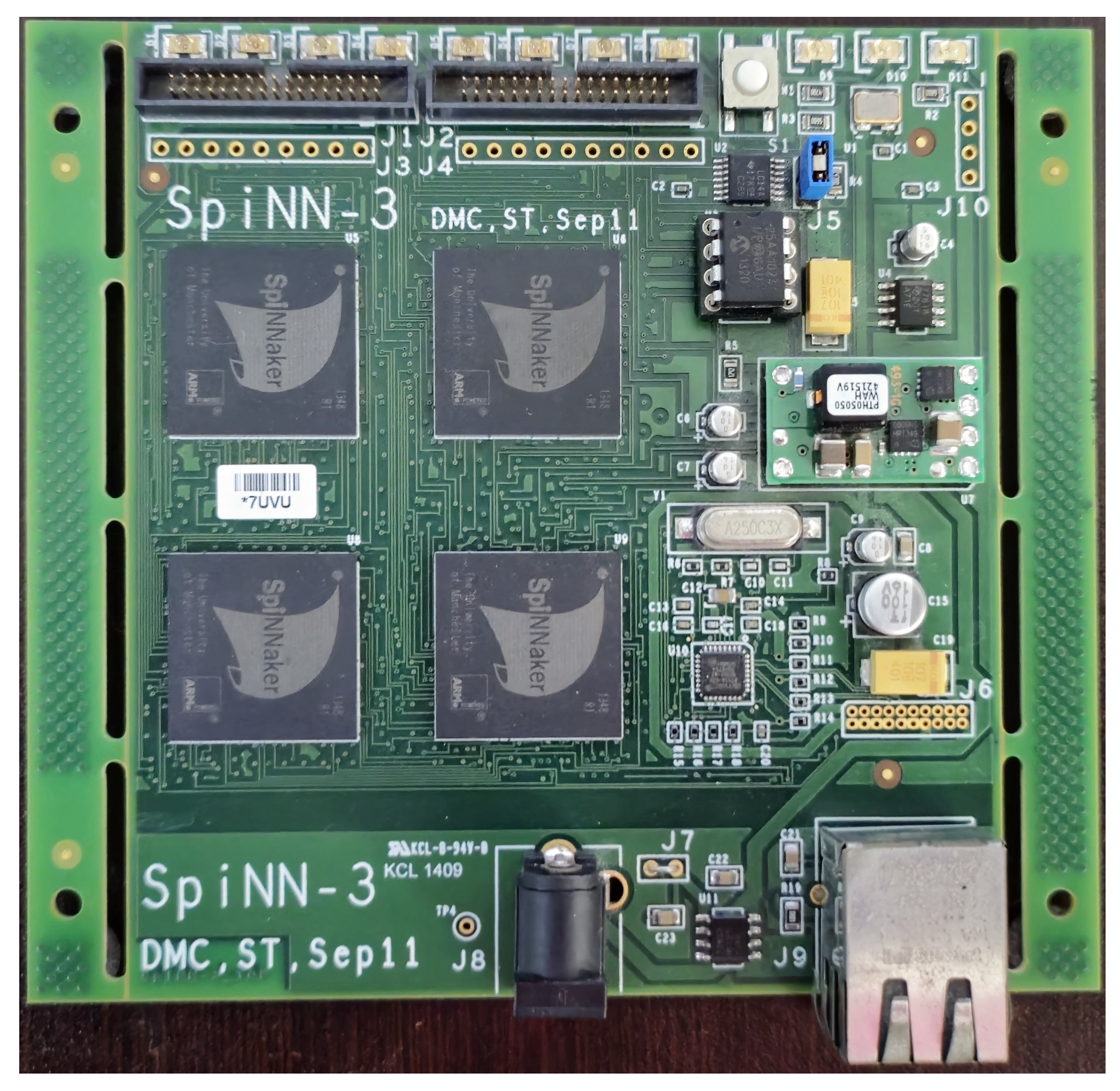
3.5. Implementation on Neuromorphic SpiNNaker Hardware

The SpiNNaker system is a multicore computing platform specifically engineered to simulate the behavior of up to a billion spiking neurons in real time [36]. At the heart of SpiNNaker’s innovation is its unique communication infrastructure, optimized for transmitting large volumes of compact packets efficiently [37]. Each packet represents a ‘spike’, a discrete communication unit among neurons encoding both the originating neuron and the timing of the spike. This architecture is especially suited for handling spatio-temporal datasets.

In this study, we enhanced the reservoir’s performance by implementing metaheuristic algorithms. Subsequently, the optimized synaptic weights for the input layer and reservoir were extracted and deployed onto the SpiNNaker system. These synaptic weights, encoded as 16-bit fixed-point values, are subject to range constraints determined at the compile time. This limitation affects the precision of synaptic weights, as the smallest representable value depends on the largest specified weight [37]. For the simulation, a scale factor of 1 ms per step was used, as increasing the scale did not yield performance improvements.

Our work utilized the SpiNNaker-3 board, illustrated in Figure 5. This board integrated 4 SpiNNaker chips, each containing 18 ARM968 processing cores with dedicated local memory, allowing each core to support one or more neurons while maintaining low power consumption. Additionally, each chip had access to 1 GB (128 MB) of SDRAM. The board connected to a host machine via an RJ45 Ethernet port, which facilitated code downloads and real-time system communication at 10 or 100 Mbit/s [38].

4. Results

The different experiments focused on evaluating the LSM, primarily assessing the reservoir’s ability to discriminate samples from each dataset. Four datasets were considered for the LSM evaluation: FR5, PR4, PR8, and PR12. Each experiment was conducted with variations in synaptic connectivity, leading to greater heterogeneity in the reservoir and influencing each optimization process. For each experiment, we gathered information from both the initial state (before optimization) and the final state (after optimization), considering the following characteristics:

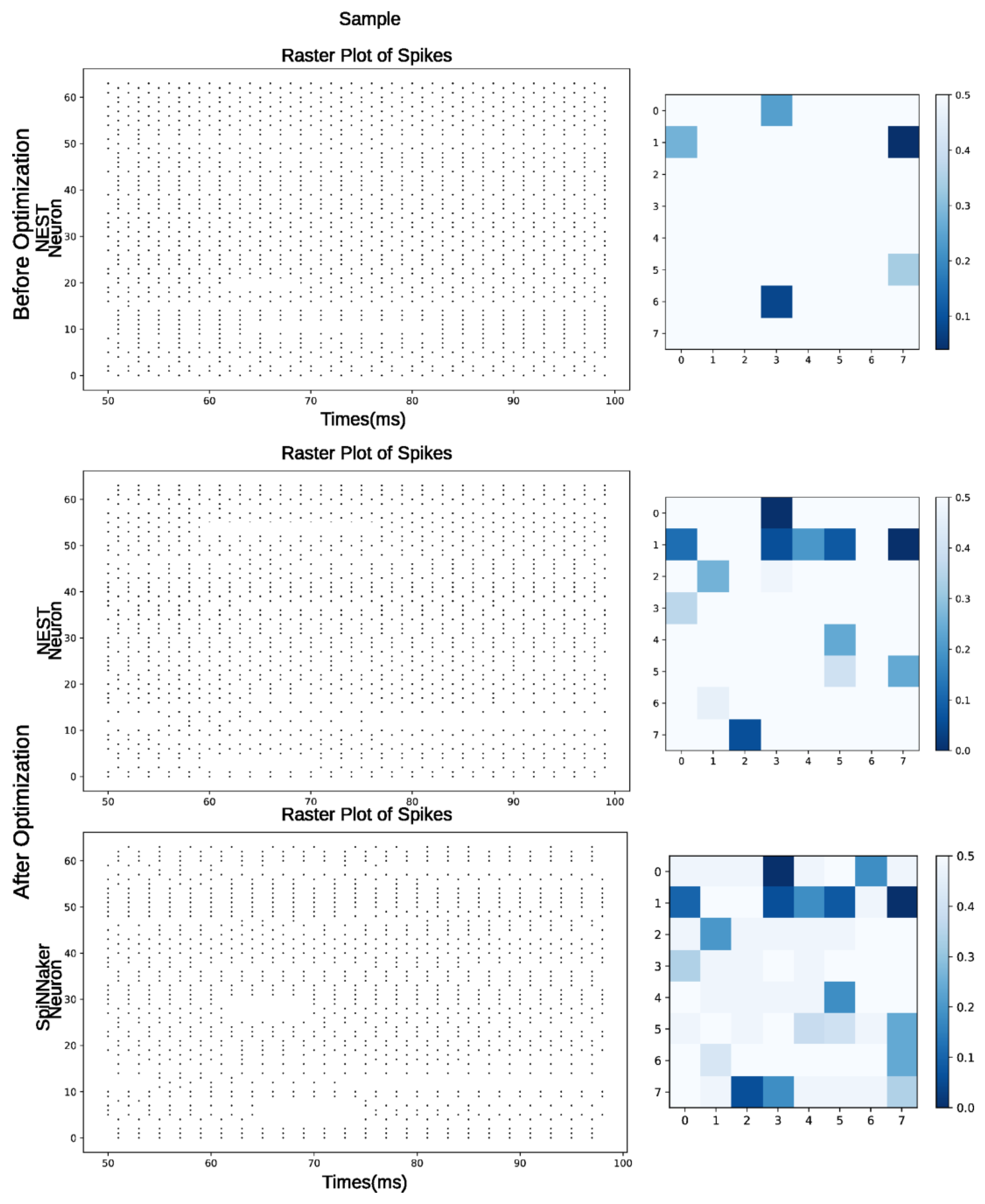
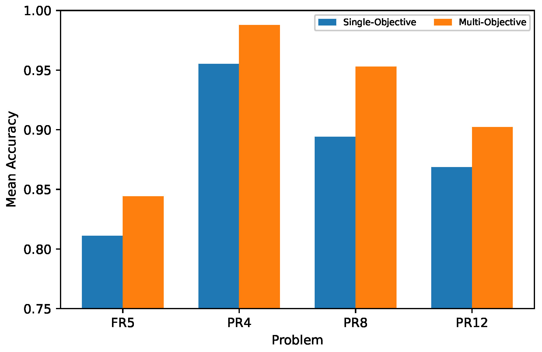
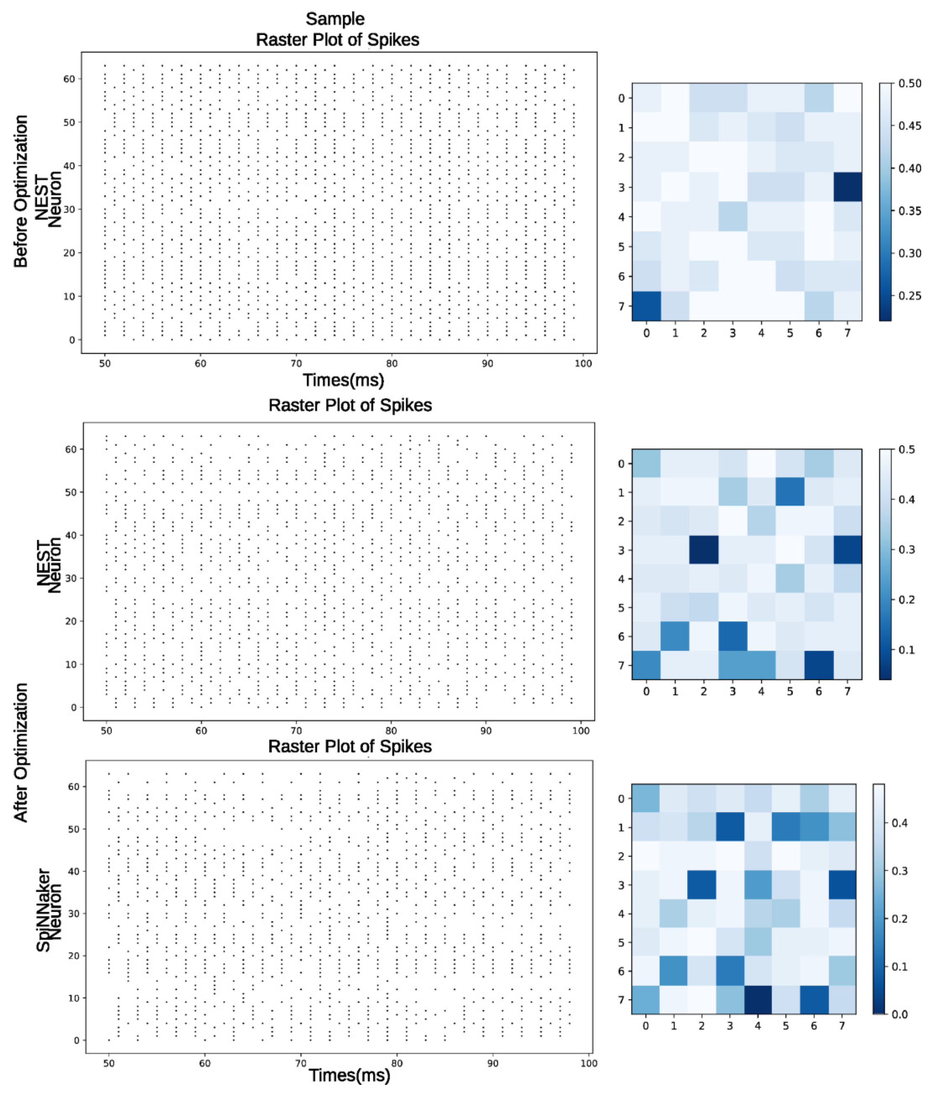
• Initial Separability (InitialSP) and Final Separability (FinalSP), which represent how well the liquid states generated by the reservoir could be separated based on the classes, in one or more tasks, before and after optimization, respectively.
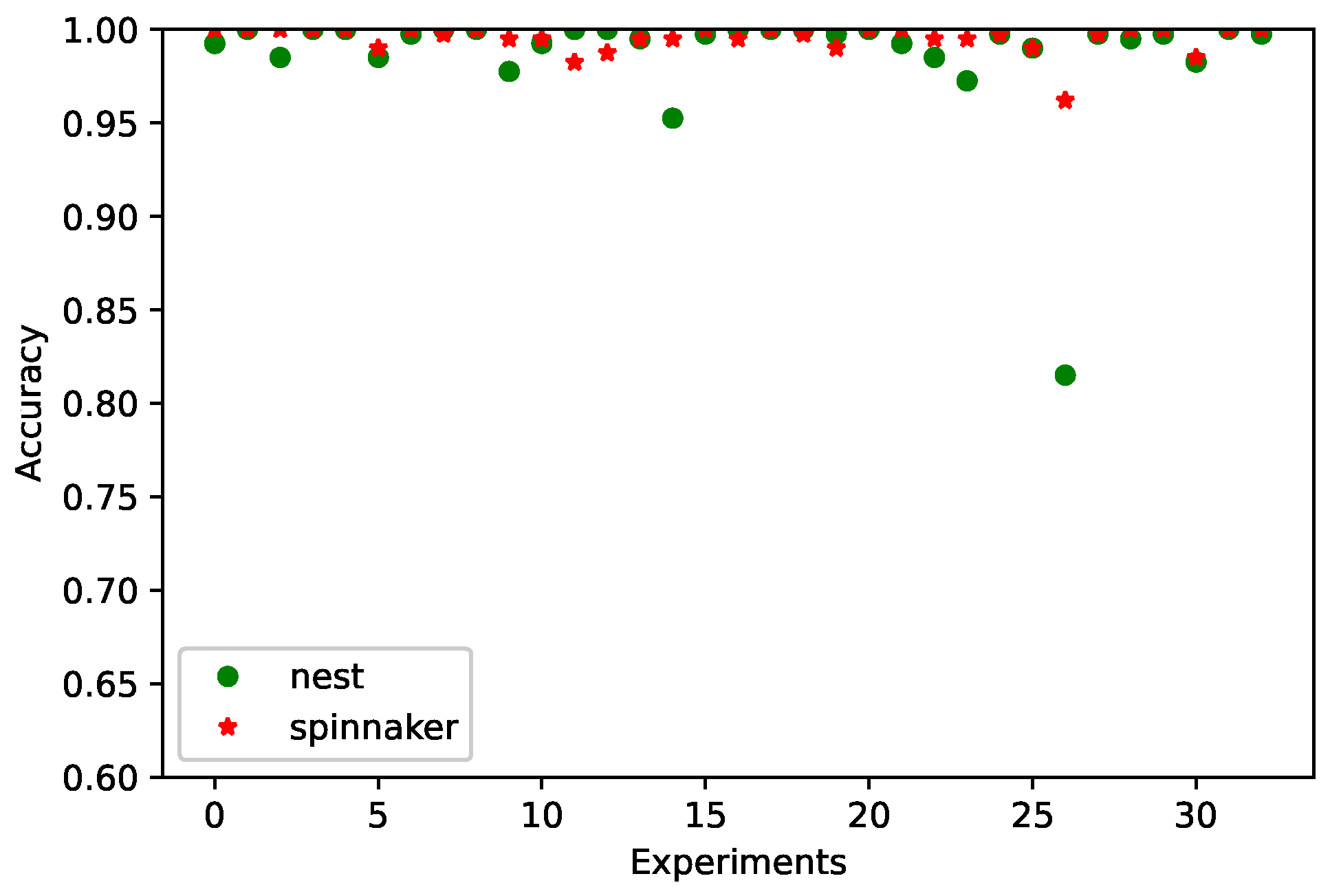
• Initial Accuracy (InitialAcc) and Final Accuracy (FinalAcc), which indicate the model’s performance when evaluated using the test datasets in NEST.
• Final Accuracy Hardware (FinalAccHW), which represents the model’s performance when simulated on SpiNNaker.

In the SpiNNaker implementations, we only evaluated FinalAcc and assess its behavior based on the results obtained in NEST.

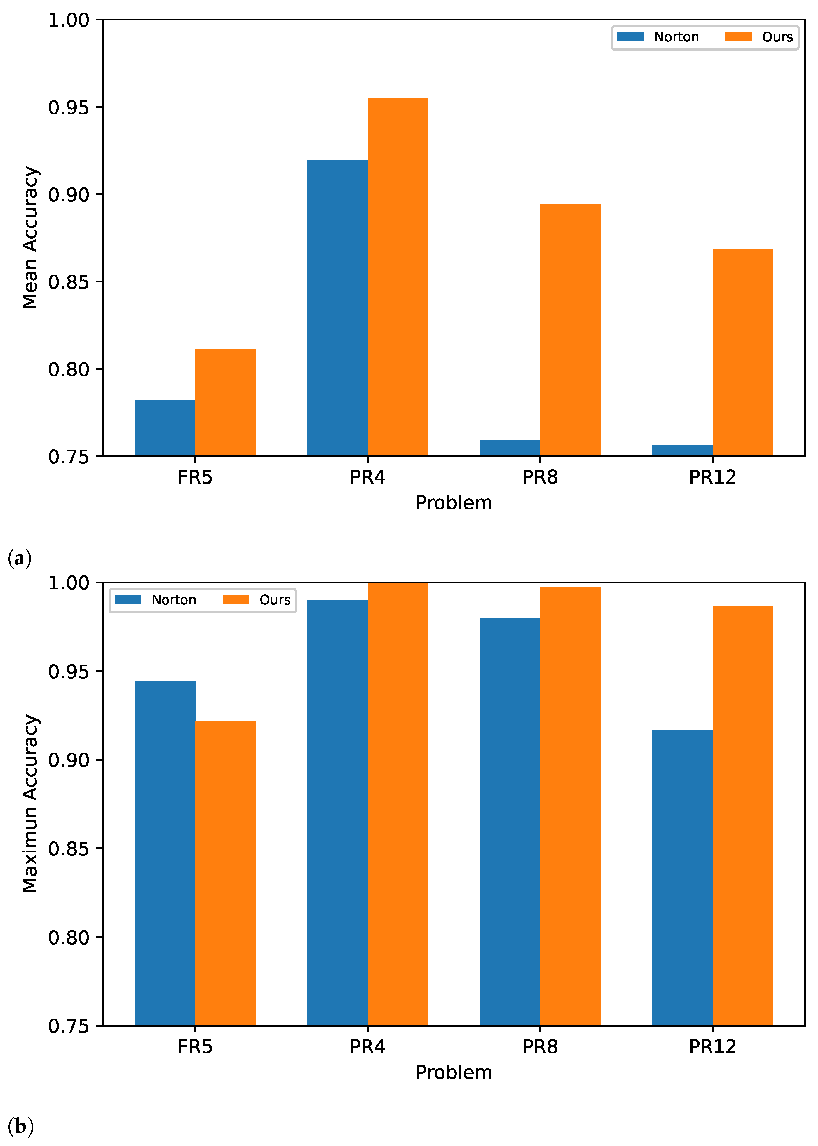
4.1. PSO Experiments

In this section, we review the results obtained from implementing PSO in the LSM with four tasks simulated independently in NEST and the migration of the synaptic weights of interest to SpiNNaker. For the optimization process simulations, we used the Pymoo framework [39] with the following parameters: a population size of 25, an inertia weight of 0.9 applied in each iteration for velocity updates, a cognitive acceleration factor of 2.0, a social acceleration factor of 2.0, a randomly initialized velocity, and mutation applied to the global best.

In

Table 2. Statistics derived from the 33 single-objective experiments.

Dataset	Statistical	InitialSP	FinalSP	InitialAcc	FinalAcc	FinalAccHW
FR5	$\overline{x}$	0.1095	0.3524	0.4931	0.8109	0.8620
	$\tilde{x}$	0.1142	0.3568	0.4820	0.8260	0.8740
	$\sigma$	0.0828	0.1303	0.2056	0.0846	0.0581
PR4	$\overline{x}$	0.0772	0.3057	0.7138	0.9552	0.9770
	$\tilde{x}$	0.0700	0.2859	0.7825	0.9875	0.9925
	$\sigma$	0.0544	0.1086	0.2065	0.0784	0.0358
PR8	$\overline{x}$	0.0697	0.3508	0.5263	0.8940	0.9432
	$\tilde{x}$	0.0729	0.3640	0.5888	0.9425	0.9613
	$\sigma$	0.0442	0.1412	0.2308	0.1199	0.0583
PR12	$\overline{x}$	0.0750	0.3079	0.4697	0.8687	0.9177
	$\tilde{x}$	0.0737	0.3056	0.4975	0.9033	0.9442
	$\sigma$	0.0426	0.1072	0.1829	0.0905	0.0662

, we can see how $\overline{x}$ and $\tilde{x}$ represent a significant improvement when considering the initial and final phases of the experiments in terms of InitialSP–FinalSP and InitialAcc–FinalAcc. This ensures a smaller $\sigma$ value after the optimization process for each of the tasks, guaranteeing the proper behavior of the process. Taking the median as the reference performance value, the quantitative range of difference between the NEST and SpiNNaker results with the PSO optimization method is 0.043. This indicates, in the context of accuracy classification, that there is a small difference between all the results from both implementations.

In Table 2 and

Table 3. Statistics derived from the 33 multi-objective experiments.

Dataset	Statistical	Initial SP	Final SP	Initial Acc	Final Acc	Final Acc HW
FR5	$\overline{x}$	0.1199	0.3557	0.5555	0.8440	0.8853
	$\tilde{x}$	0.1136	0.3658	0.5740	0.8880	0.9000
	$\sigma$	0.0712	0.0863	0.1948	0.0886	0.0392
PR4	$\overline{x}$	0.0764	0.2325	0.7796	0.9877	0.9952
	$\tilde{x}$	0.0686	0.2255	0.7989	0.9975	0.9975
	$\sigma$	0.0475	0.0502	0.1895	0.0327	0.0077
PR8	$\overline{x}$	0.0859	0.2311	0.6179	0.9529	0.9706
	$\tilde{x}$	0.0807	0.2234	0.6405	0.9712	0.9750
	$\sigma$	0.0479	0.0439	0.2057	0.0411	0.0158
PR12	$\overline{x}$	0.0883	0.2414	0.5165	0.9023	0.9442
	$\tilde{x}$	0.0895	0.2342	0.5358	0.9200	0.9520
	$\sigma$	0.0474	0.0472	0.2110	0.0537	0.0257

, the primary focus is not on comparing FinalACC and FinalACCHW but rather on comparing these metrics with InitialACC. This comparison reveals a significant improvement, demonstrating the effectiveness of our approach. Additionally, it is important to consider the separability measures, which further highlight the enhanced performance of our method. This is true for both the single-objective and multi-objective problems. The goal was to ensure that FinalACC and FinalACCHW exhibited similar performance, as this would indicate that our method was effective and consistent across both software and hardware implementations. Achieving comparable results with both platforms highlights the robustness and adaptability of our approach, showcasing its potential for practical applications. Furthermore, SpiNNaker operates at around 1–5 watts per chip, while traditional systems can require 50–100 watts for similar tasks [40], emphasizing the significant energy efficiency advantage of our hardware-based solution.

Figure 6a shows the performance improvement in the reservoir in each task compared to the results obtained in [14], based on accuracy (Acc), with less precision in the synaptic weights. Additionally, we were able to exceed the maximum accuracy achieved in three of the tasks compared to the total experiments, as shown in Figure 6b.

The SpiNNaker implementation is represented by FinalAccHW, where a difference is observed compared to FinalAcc, particularly in FR5, which corresponds to the task with the lowest FinalAcc. This highlights how the reservoir’s separability and an adequate firing rate influenced the performance of the implementation on SpiNNaker. If the firing rate is too high, it may not be possible to process all spikes in each time step in a real-world environment due to the inherent architecture of the hardware.

In Figure 7, we observe the behavior of each experiment both in NEST and on SpiNNaker after the optimization process. In certain experiments, such as 4, 14, and 26, the single-objective optimization on SpiNNaker demonstrated improved accuracy compared to simulations conducted in NEST. This improvement is likely attributable to the hardware-specific advantages of SpiNNaker, a neuromorphic platform designed to emulate spiking neural networks with high efficiency. Unlike traditional simulators, SpiNNaker’s asynchronous architecture and real-time spike processing closely mirror biological neural dynamics, enabling more precise temporal interactions within a Liquid State Machine (LSM). These characteristics contribute to enhanced reservoir separability and stability, which are critical for improving classification performance in spatio-temporal tasks. The reduced latency and optimized handling of spikes on SpiNNaker further support its suitability for implementing LSMs, leading to notable gains in performance under specific experimental conditions. A similar situation occurred with the multi-objective optimization, as will be seen below.

In Figure 8, we can observe the behavior of the liquid state based on a simulated sample from the last 50 ms in three stages, each represented by a raster plot and a heatmap: The first corresponds to Before Optimization, where we observed the liquid state behavior before optimization, simulated in NEST, where the reservoir showed a high firing rate. In After Optimization—NEST, we observed the behavior of the reservoir after the optimization process, simulated in NEST, resulting in a slightly more regularized firing pattern. Finally, After Optimization—SpiNNaker represents the behavior of the reservoir simulated on the hardware, showing a pattern very similar to the one obtained in NEST after optimization. Focusing on the heatmap, which is a representation of the liquid state, we can observe the effect of the separability-based optimization process, where the liquid’s neurons neither overreacted nor reacted similarly to any stimuli, allowing for an enhanced overall LSM performance.

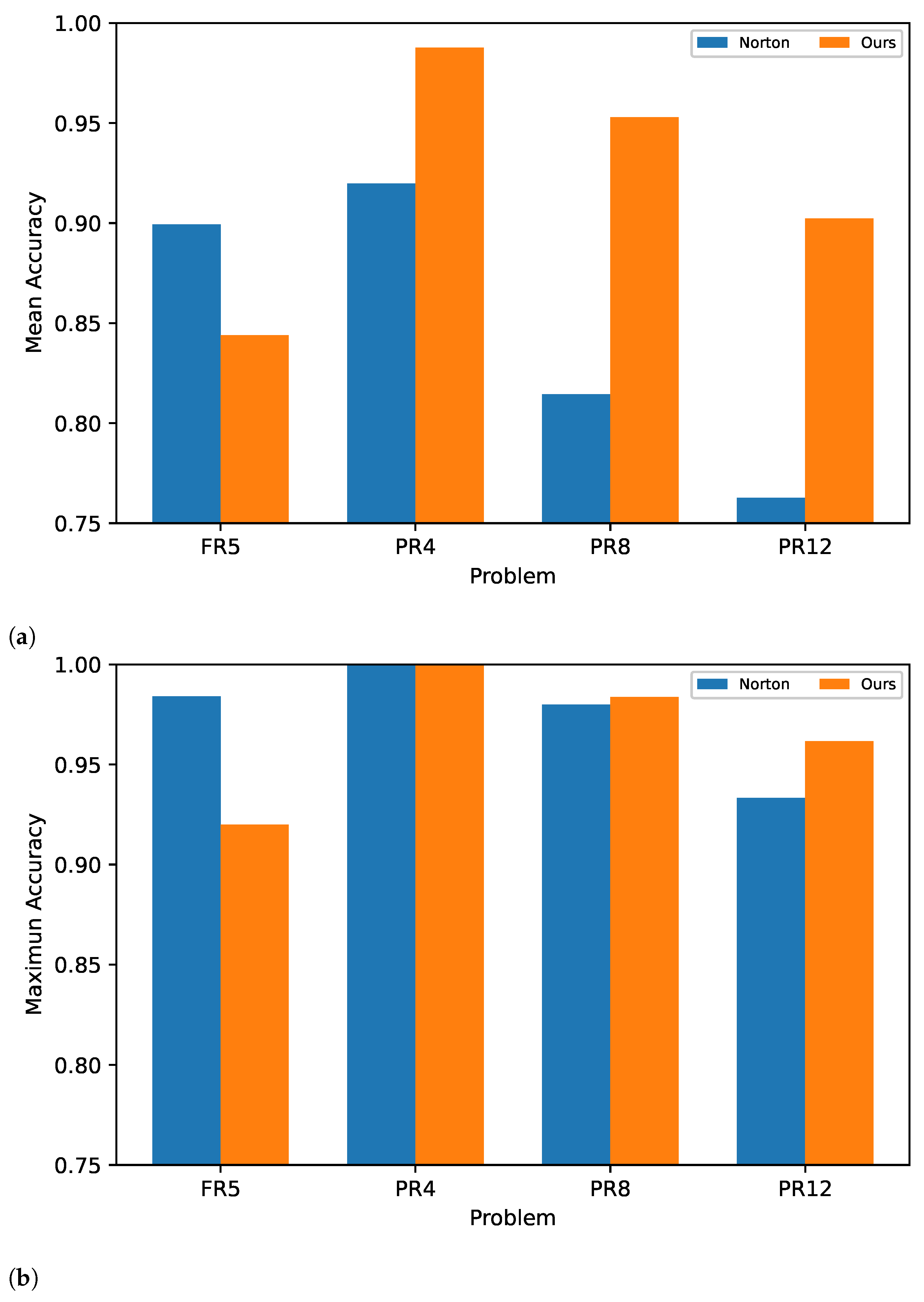
4.2. OMOPSO Experiments

In this section, we review the results of implementing OMOPSO in the LSM with four tasks simultaneously simulated in NEST and the migration of the synaptic weights of interest to SpiNNaker. For the optimization simulations, we used the Jmetalpy framework (https://github.com/jMetal/jMetalPy, accessed on 22 october 2024) with the following parameters: a swarm size of 25 particles, a mutation probability of 1/|variables|, an $ϵ$ factor of 0.075, a crowding distance archive of 25 leaders, and a maximum evaluation stopping criterion of 500 evaluations. These parameters were determined through empirical evidence.

In Table 3, we observe, just like in the PSO implementation, an improvement after the optimization process considering InitialSP–FinalSP and InitialAcc–FinalAcc. This improvement is reflected in the statistics $\overline{x}$ and $\tilde{x}$, where an increasing trend can be seen between the initial and final states of the reservoir. Additionally, the value of $\sigma$ decreases in each task, demonstrating consistency in the reservoir’s performance. Similarly to PSO, for the case of the OMOPSO optimizer, we considered the median as the reference performance value to calculate the quantitative range of difference between the NEST and SpiNNaker results. This gave a value of 0.032, which similarly reflects that there is a small difference between all the results from both implementations, even smaller than the results obtained by using PSO.

In Figure 9a, we can see that the reservoir performance improved in most of the implemented tasks, specifically in PR4, PR8, and PR12, compared to the results in [14], with the exception of FR5. However, for FR5, we achieved a higher $\overline{x}$ performance than in the mono-objective case, with a lower $\sigma$ value. From the above, we can observe how FR5 may have been influenced by “optimization conformity” during the training process, where solutions were generated to benefit the majority of tasks. This suggests an underrepresentation of the FR5 task. In Figure 9b, the maximum accuracy obtained from the 33 experiments across the four tasks is shown. The results demonstrate acceptable performance in most tasks, with FR5 achieving a performance consistent with the mean accuracy.

The values used for comparison were obtained from [14] and were selected for each task based on the highest average performance, $\overline{x}$, after evaluating them in each base reservoir. This reservoir was considered for transferring learning to the other tasks. The results from the SpiNNaker implementation are shown in FinalAccHW, where a smaller difference between FinalAcc and FinalAccHW can be observed compared to the mono-objective case, based on the model’s average performance. In Figure 10, we can see $\overline{x}$ for each experiment using NEST and SpiNNaker, showing an improvement in the model’s performance dispersion, indicating appropriate behavior even with high spike rates. Although the final stage of the multi-objective optimization process did not result in a higher $\overline{x}$ for FR5, it is evident that this method outperformed all tasks when optimized independently, as seen in Figure 11, allowing for improved reservoir performance and reduced training time.

In Figure 12, we observe the liquid state behavior based on a sample considering the last 50 ms of simulation, with the corresponding heatmap. This process involved three stages: The first, labeled “Before Optimization”, was simulated with NEST, showing the initial behavior of the reservoir without implementing any strategies to improve its performance. This stage was characterized by a high spike rate. “After Optimization—NEST” represents the reservoir’s behavior after the optimization process, where a lower spike rate was observed. This is reflected in the heatmap, where some neurons reduce their spike frequency, further regularizing the reservoir’s behavior. “After Optimization—SpiNNaker” shows the behavior obtained by implementing the hardware, where we observe that some neurons further reduce their spike frequency.

Both in mono-objective and multi-objective optimizations, the SpiNNaker implementation showed a slight reduction in the spike rate, even in simulations with high spike frequency, when compared to the NEST implementation. This highlights the excellent performance of the hardware and the challenges we encountered, such as the noise generated by the hardware itself due to asynchronous core synchronization, the fine-tuning required through metaheuristic implementation, and the scalability of the weight representation in the hardware, among others. A significant limitation for not running the optimization process directly on the hardware was the amount of available memory for execution, which would become an even greater constraint for multi-objective implementations.

4.3. Statistical Significance Test

To validate our results, both in software (NEST simulator) and hardware (SpiNNaker board), we proceeded to perform individual statistical tests according to the used optimization method to verify whether the behavior of both implementations had the same quality or if there was any statistically significant difference and to determine which implementation was better [41].

For both optimization methods, PSO and OMOPSO, the first step was to conduct Shapiro–Wilk normality tests [42,43] to determine the distribution of their results for each implementation and dataset. The results from each dataset provided by both implementations for each optimization methods showed that none of them followed a normal distribution, which led us to perform the Wilcoxon signed-rank non-parametric test [41,44]. Next, for each optimization method and implementation (NEST or SpiNNaker), the median value for each result set per benchmark dataset was calculated as a reference value to perform the Wilcoxon signed-rank test; thus, the statistical test for each optimization method included two implementations with four paired samples.

For the PSO optimization method, the results of the Wilcoxon signed-rank test were used to compare the performance of the two implementations, one in NEST and the other in SpiNNaker. The test statistic (V) was 0, with a p-value of 0.125. Since the p-value was greater than the used significance level of 0.05, we failed to reject the null hypothesis. This suggests that there was no statistically significant difference between the two implementations.

For the OMOPSO optimization methods, the results of the Wilcoxon signed-rank test were applied to compare the two implementations, one in NEST and the other in SpiNNaker. The test statistic (V) was 0, with a p-value of 0.25. Given that the p-value exceeded the significance level of 0.05, we failed to reject the null hypothesis.

From both statistical tests, we can conclude that the software and hardware implementations had similar performances with respect to the median accuracy. Thus, there was no decrease in performance when software implementations were migrated to hardware.

5. Conclusions

In this work, we proposed and validated an optimization approach based on Particle Swarm Optimization (PSO) to enhance reservoir separability in Liquid State Machines (LSMs), specifically for spatio-temporal classification tasks with neuromorphic systems. The experimental results demonstrated significant improvements in classification accuracy and computational efficiency, validating the implementation on the SpiNNaker neuromorphic platform. For example, with the Mono-objective approach, average performance improvements in benchmark problems such as FR5, PR4, PR8, and PR12 were achieved, with values of 86.2%, 97.7%, 94.32%, and 91.77%, respectively. Additionally, the multi-objective approach delivered exceptional results with 88.53%, 99.52%, 97.06%, and 94.42% in the same problems, consistently outperforming the Mono-objective approach. Although for both optimization methods there were no significant statistical differences in accuracy between the performance of the NEST simulator and the SpiNNaker board, the superiority of the neuromorphic platform became evident in implementation aspects, such as the reported processing time comparisons [45].

A key aspect of this work is that SpiNNaker not only allows embedded implementations based on spiking neural networks but also does so with significantly lower power consumption compared to traditional systems like NEST [45,46]. This energy efficiency, coupled with real-time simulation capabilities, positions SpiNNaker as an ideal platform for the scalable implementation of LSMs.

Furthermore, PSO-optimized reservoir configurations not only improved sample separability but also reduced the neuron spike rate, contributing to more regular and efficient reservoir behavior, despite the technical challenges of the hardware. This approach is scalable and adaptable, allowing implementation on other neuromorphic platforms such as TruNorth [47] and Loihi [48], which also provide energy-efficient processing for spiking neural networks.

The robustness of our approach lies in its versatility, as the model can be directly implemented both in software and hardware, without requiring significant modifications. This dual applicability ensures that the solution is adaptable to a variety of deployment environments, from traditional computational platforms to specialized neuromorphic hardware. When implemented in software, the model can take advantage of the flexibility and scalability provided by general-purpose computing systems, allowing for fast prototyping and testing across different configurations and datasets. On the other hand, when deployed on neuromorphic hardware like SpiNNaker, TruNorth, or Loihi, the model benefits from the inherent efficiency and low power consumption of these platforms, enabling the real-time processing of spatio-temporal signals with minimal energy demands. This ability to seamlessly transition between software and hardware implementations not only enhances the practicality of the approach but also broadens its potential applications, making it a robust solution for both research and real-world use cases in fields such as biomedical signal processing, intelligent surveillance, and brain–computer interfaces.

In conclusion, this work marks an important step toward the optimization and scalability of LSMs on neuromorphic systems. The improvements in performance, energy efficiency, and accuracy highlight the potential of PSO as an effective tool for fully exploiting the capabilities of neuromorphic hardware. This approach benefits from envisioning suitable paths for overcoming current limitations and expanding the practical applications of LSMs on platforms such as SpiNNaker, TruNorth, and Loihi.

References

1. Budhraja, S.; Singh, B.; Doborjeh, M.; Doborjeh, Z.; Tan, S.; Lai, E.; Goh, W.; Kasabov, N. Mosaic LSM: A Liquid State Machine Approach for Multimodal Longitudinal Data Analysis. In Proceedings of the 2023 International Joint Conference on Neural Networks (IJCNN), Gold Coast, Australia, 18–23 June 2023; pp. 1–8. [Google Scholar] [CrossRef]
2. Sai Sree Vaishnavi, V.G.; Bhowmik, B. Evolution of Neuromorphic Computing. In Proceedings of the 2024 Fourth International Conference on Advances in Electrical, Computing, Communication and Sustainable Technologies (ICAECT), Bhilai, India, 11–12 January 2024; pp. 1–8. [Google Scholar] [CrossRef]
3. Schuman, C.D.; Kulkarni, S.R.; Parsa, M.; Mitchell, J.P.; Date, P.; Kay, B. Opportunities for neuromorphic computing algorithms and applications. Nat. Comput. Sci. 2022, 2, 10–19. [Google Scholar] [CrossRef]
4. Tian, S.; Qu, L.; Wang, L.; Hu, K.; Li, N.; Xu, W. A neural architecture search based framework for liquid state machine design. Neurocomputing 2021, 443, 174–182. [Google Scholar] [CrossRef]
5. Woo, J.; Kim, S.H.; Kim, H.; Han, K. Characterization of the neuronal and network dynamics of liquid state machines. Phys. A Stat. Mech. Its Appl. 2024, 633, 129334. [Google Scholar] [CrossRef]
6. Pan, W.; Zhao, F.; Zeng, Y.; Han, B. Adaptive structure evolution and biologically plausible synaptic plasticity for recurrent spiking neural networks. Sci. Rep. 2023, 13, 16924. [Google Scholar] [CrossRef] [PubMed]
7. Wijesinghe, P.; Srinivasan, G.; Panda, P.; Roy, K. Analysis of Liquid Ensembles for Enhancing the Performance and Accuracy of Liquid State Machines. Front. Neurosci. 2019, 13, 504. [Google Scholar] [CrossRef] [PubMed]
8. Patel, R.; Saraswat, V.; Ganguly, U. Liquid State Machine on Loihi: Memory Metric for Performance Prediction. In Artificial Neural Networks and Machine Learning—ICANN 2022; Pimenidis, E., Angelov, P., Jayne, C., Papaleonidas, A., Aydin, M., Eds.; Springer Nature: Cham, Switzerland, 2022; pp. 692–703. [Google Scholar]
9. Patiño-Saucedo, A.; Rostro-González, H.; Serrano-Gotarredona, T.; Linares-Barranco, B. Liquid State Machine on SpiNNaker for Spatio-Temporal Classification Tasks. Front. Neurosci. 2022, 16, 819063. [Google Scholar] [CrossRef] [PubMed]
10. Wang, L.; Yang, Z.; Guo, S.; Qu, L.; Zhang, X.; Kang, Z.; Xu, W. LSMCore: A 69k-Synapse/mm2 Single-Core Digital Neuromorphic Processor for Liquid State Machine. IEEE Trans. Circuits Syst. I Regul. Pap. 2022, 69, 1976–1989. [Google Scholar] [CrossRef]
11. Norton, D.; Ventura, D. Improving the separability of a reservoir facilitates learning transfer. In Proceedings of the 2009 International Joint Conference on Neural Networks, Atlanta, GA, USA, 14–19 June 2009; pp. 2288–2293. [Google Scholar] [CrossRef]
12. Ortman, R.L.; Venayagamoorthy, K.; Potter, S.M. Input Separability in Living Liquid State Machines. In Adaptive and Natural Computing Algorithms; Dobnikar, A., Lotrič, U., Šter, B., Eds.; Springer: Berlin/Heidelberg, Germany, 2011; pp. 220–229. [Google Scholar]
13. Zhou, Y.; Jin, Y.; Ding, J. Evolutionary Optimization of Liquid State Machines for Robust Learning. In Advances in Neural Networks—ISNN 2019; Lu, H., Tang, H., Wang, Z., Eds.; Springer International Publishing: Cham, Switzerland, 2019; pp. 389–398. [Google Scholar]
14. Norton, D.; Ventura, D. Improving liquid state machines through iterative refinement of the reservoir. Neurocomputing 2010, 73, 2893–2904. [Google Scholar] [CrossRef]
15. Mehonic, A.; Ielmini, D.; Roy, K.; Mutlu, O.; Kvatinsky, S.; Serrano-Gotarredona, T.; Linares-Barranco, B.; Spiga, S.; Savel’ev, S.; Balanov, A.G.; et al. Roadmap to neuromorphic computing with emerging technologies. APL Mater. 2024, 12, 109201. [Google Scholar] [CrossRef]
16. Sandamirskaya, Y.; Kaboli, M.; Conradt, J.; Celikel, T. Neuromorphic computing hardware and neural architectures for robotics. Sci. Robot. 2022, 7, eabl8419. [Google Scholar] [CrossRef] [PubMed]
17. Cucchi, M.; Abreu, S.; Ciccone, G.; Brunner, D.; Kleemann, H. Hands-on reservoir computing: A tutorial for practical implementation. Neuromorphic Comput. Eng. 2022, 2, 032002. [Google Scholar] [CrossRef]
18. Zhou, Y.; Jin, Y.; Sun, Y.; Ding, J. Surrogate-Assisted Cooperative Co-evolutionary Reservoir Architecture Search for Liquid State Machines. IEEE Trans. Emerg. Top. Comput. Intell. 2023, 7, 1484–1498. [Google Scholar] [CrossRef]
19. Yan, M.; Huang, C.; Bienstman, P.; Tino, P.; Lin, W.; Sun, J. Emerging opportunities and challenges for the future of reservoir computing. Nat. Commun. 2024, 15, 2056. [Google Scholar] [CrossRef] [PubMed]
20. Orchard, G.; Jayawant, A.; Cohen, G.K.; Thakor, N. Converting static image datasets to spiking neuromorphic datasets using saccades. Front. Neurosci. 2015, 9, 437. [Google Scholar] [CrossRef] [PubMed]
21. Maass, W. Liquid State Machines: Motivation, Theory, and Applications. In Computability in Context; World Scientific: Singapore, 2011; pp. 275–296. [Google Scholar] [CrossRef]
22. Maass, W.; Natschläger, T.; Markram, H. Real-time computing without stable states: A new framework for neural computation based on perturbations. Neural Comput. 2002, 14, 2531–2560. [Google Scholar] [CrossRef]
23. Norton, D.; Ventura, D. Preparing more effective liquid state machines using hebbian learning. In Proceedings of the 2006 IEEE International Joint Conference on Neural Network Proceedings, Vancouver, BC, Canada, 16–21 July 2006; pp. 4243–4248. [Google Scholar]
24. Zhang, H.; Vargas, D.V. A survey on reservoir computing and its interdisciplinary applications beyond traditional machine learning. IEEE Access 2023, 11, 81033–81070. [Google Scholar] [CrossRef]
25. Shen, S.; Zhang, R.; Wang, C.; Huang, R.; Tuerhong, A.; Guo, Q.; Lu, Z.; Zhang, J.; Leng, L. Evolutionary spiking neural networks: A survey. J. Membr. Comput. 2024, 6, 335–346. [Google Scholar] [CrossRef]
26. Kennedy, J.; Eberhart, R. Particle swarm optimization. In Proceedings of the ICNN’95-International Conference on Neural Networks, Perth, Australia, 27 November–1 December 1995; Volume 4, pp. 1942–1948. [Google Scholar]
27. Shami, T.M.; El-Saleh, A.A.; Alswaitti, M.; Al-Tashi, Q.; Summakieh, M.A.; Mirjalili, S. Particle swarm optimization: A comprehensive survey. IEEE Access 2022, 10, 10031–10061. [Google Scholar] [CrossRef]
28. Sierra, M.R.; Coello Coello, C.A. Improving PSO-based multi-objective optimization using crowding, mutation and ϵ-dominance. In Evolutionary Multi-Criterion Optimization, Proceedings of the Third International Conference, EMO 2005, Guanajuato, Mexico, 9–11 March 2005; Springer: Berlin/Heidelberg, Germany, 2005; pp. 505–519. [Google Scholar]
29. Coello, C.A.C.; Pulido, G.T.; Lechuga, M.S. Handling multiple objectives with particle swarm optimization. IEEE Trans. Evol. Comput. 2004, 8, 256–279. [Google Scholar] [CrossRef]
30. Gewaltig, M.O.; Diesmann, M. NEST (NEural Simulation Tool). Scholarpedia 2007, 2, 1430. [Google Scholar] [CrossRef]
31. Davison, A.P.; Brüderle, D.; Eppler, J.M.; Kremkow, J.; Muller, E.; Pecevski, D.; Perrinet, L.; Yger, P. PyNN: A common interface for neuronal network simulators. Front. Neuroinform. 2009, 2, 388. [Google Scholar] [CrossRef]
32. Trelea, I.C. The particle swarm optimization algorithm: Convergence analysis and parameter selection. Inf. Process. Lett. 2003, 85, 317–325. [Google Scholar] [CrossRef]
33. van den Bergh, F.; Engelbrecht, A. A Cooperative approach to particle swarm optimization. IEEE Trans. Evol. Comput. 2004, 8, 225–239. [Google Scholar] [CrossRef]
34. Zhang, L.; Yu, H.; Hu, S. Optimal choice of parameters for particle swarm optimization. J. Zhejiang-Univ.-Sci. A 2005, 6, 528–534. [Google Scholar]
35. Poli, R.; Kennedy, J.; Blackwell, T. Particle swarm optimization. Swarm Intell. 2007, 1, 33–57. [Google Scholar] [CrossRef]
36. Indiveri, G.; Liu, S.C. Memory and information processing in neuromorphic systems. Proc. IEEE 2015, 103, 1379–1397. [Google Scholar] [CrossRef]
37. Furber, S.B.; Galluppi, F.; Temple, S.; Plana, L.A. The spinnaker project. Proc. IEEE 2014, 102, 652–665. [Google Scholar] [CrossRef]
38. Temple, S. AppNote 1-SpiNN-3 Development Board; The University of Manchester: Manchester, UK, 2011; Volume 1. [Google Scholar]
39. Blank, J.; Deb, K. Pymoo: Multi-objective optimization in python. IEEE Access 2020, 8, 89497–89509. [Google Scholar] [CrossRef]
40. Painkras, E.; Plana, L.A.; Garside, J.; Temple, S.; Galluppi, F.; Patterson, C.; Lester, D.R.; Brown, A.D.; Furber, S.B. SpiNNaker: A 1-W 18-Core System-on-Chip for Massively-Parallel Neural Network Simulation. IEEE J.-Solid-State Circuits 2013, 48, 1943–1953. [Google Scholar] [CrossRef]
41. Flach, P. Machine Learning: The Art and Science of Algorithms That Make Sense of Data; Cambridge University Press: Cambridge, UK, 2012. [Google Scholar]
42. Ghasemi, A.; Zahediasl, S. Normality tests for statistical analysis: A guide for non-statisticians. Int. J. Endocrinol. Metab. 2012, 10, 486. [Google Scholar] [CrossRef] [PubMed]
43. Grech, V.; Calleja, N. WASP (Write a Scientific Paper): Parametric vs. non-parametric tests. Early Hum. Dev. 2018, 123, 48–49. [Google Scholar] [CrossRef] [PubMed]
44. Derrac, J.; García, S.; Molina, D.; Herrera, F. A practical tutorial on the use of nonparametric statistical tests as a methodology for comparing evolutionary and swarm intelligence algorithms. Swarm Evol. Comput. 2011, 1, 3–18. [Google Scholar] [CrossRef]
45. Sharp, T.; Furber, S. Correctness and performance of the SpiNNaker architecture. In Proceedings of the 2013 International Joint Conference on Neural Networks (IJCNN), Dallas, TX, USA, 4–9 August 2013; pp. 1–8. [Google Scholar]
46. van Albada, S.J.; Rowley, A.G.; Senk, J.; Hopkins, M.; Schmidt, M.; Stokes, A.B.; Lester, D.R.; Diesmann, M.; Furber, S.B. Performance Comparison of the Digital Neuromorphic Hardware SpiNNaker and the Neural Network Simulation Software NEST for a Full-Scale Cortical Microcircuit Model. Front. Neurosci. 2018, 12, 291. [Google Scholar] [CrossRef] [PubMed]
47. Akopyan, F.; Sawada, J.; Cassidy, A.; Alvarez-Icaza, R.; Arthur, J.; Merolla, P.; Imam, N.; Nakamura, Y.; Datta, P.; Nam, G.J.; et al. TrueNorth: Design and Tool Flow of a 65 mW 1 Million Neuron Programmable Neurosynaptic Chip. IEEE Trans.-Comput.-Aided Des. Integr. Circuits Syst. 2015, 34, 1537–1557. [Google Scholar] [CrossRef]
48. Davies, M.; Srinivasa, N.; Lin, T.H.; Chinya, G.; Cao, Y.; Choday, S.H.; Dimou, G.; Joshi, P.; Imam, N.; Jain, S.; et al. Loihi: A Neuromorphic Manycore Processor with On-Chip Learning. IEEE Micro 2018, 38, 82–99. [Google Scholar] [CrossRef]
Figure 1. A diagram of the proposed methodology adapted for a Liquid State Machine and its components.
Jlpea 15 00004 g001
Figure 2. PSO algorithm diagram.
Jlpea 15 00004 g002
Figure 3. OMOPSO algorithm diagram.
Jlpea 15 00004 g003
Figure 4. Raster plots of samples in (a) dataset FR5, (b) dataset PR4, (c) dataset PR8, and (d) dataset PR12.
Jlpea 15 00004 g004aJlpea 15 00004 g004b
Figure 5. The SpiNNaker board. A 4-node circuit board with 72 ARM processor cores.
Jlpea 15 00004 g005
Figure 6. (a) Average accuracy: Norton vs. our method. (b) Maximum accuracy: Norton vs. our method.
Jlpea 15 00004 g006
Figure 7. The accuracy of the 33 experiments in NEST and on SpiNNaker for the single-objective experiment with the PR4 dataset.
Jlpea 15 00004 g007
Figure 8. Raster plots (spiking activity) and heatmaps of the last 50 ms of simulation of a sample for mono-objective experiments.
Jlpea 15 00004 g008
Figure 9. (a) Average accuracy achieved by Norton and our approach in multi-objective experiments. (b) Maximum accuracy achieved by Norton and our approach in multi-objective experiments.
Jlpea 15 00004 g009
Figure 10. The accuracy of the 33 experiments in NEST and SpiNNaker for multi-objective experiments with the PR4 dataset.
Jlpea 15 00004 g010
Figure 11. Average accuracy achieved by single-objective and multi-objective methods.
Jlpea 15 00004 g011
Figure 12. Raster plots (spiking activity) and heatmaps of the last 50 ms of the simulation of a sample for multi-objective experiments.
Jlpea 15 00004 g012