Computationally Efficient Light Field Video Compression Using 5-D Approximate DCT

Abstract

Five-dimensional (5-D) light field videos (LFVs) capture spatial, angular, and temporal variations in light rays emanating from scenes. This leads to a significantly large amount of data compared to conventional three-dimensional videos, which capture only spatial and temporal variations in light rays. In this paper, we propose an LFV compression technique using low-complexity 5-D approximate discrete cosine transform (ADCT). To further reduce the computational complexity, our algorithm exploits the partial separability of LFV representations. It applies two-dimensional (2-D) ADCT for sub-aperture images of LFV frames with intra-view and inter-view configurations. Furthermore, we apply one-dimensional ADCT to the temporal dimension. We evaluate the performance of the proposed LFV compression technique using several 5-D ADCT algorithms, and the exact 5-D discrete cosine transform (DCT). The experimental results obtained with LFVs confirm that the proposed LFV compression technique provides a more than 250 times reduction in the data size with near-lossless fidelity with a peak-signal-to-noise ratio greater than 40 dB and structural similarity index greater than $0.9$. Furthermore, compared to the exact DCT, our algorithms requires approximately 10 times less computational complexity.

1. Introduction

Light rays emanating from a scene are completely defined by a seven-dimensional plenoptic function [1] that models light rays at every possible location in a three-dimensional (3-D) space $(x,y,z)$, from every possible direction $(\theta ,\varphi )$, at every wavelength $\lambda$, and at every time t. Five-dimensional (5-D) light field video (LFV) is a simplified form of the seven-dimensional plenoptic function derived with two assumptions: the intensity of a light ray does not change along its direction of propagation and the wavelength is represented by red, green, and blue (RGB) color channels [2,3]. With the first assumption, we can eliminate one space dimension, typically z, and with the second assumption, we can eliminate the wavelength. Therefore, an LFV corresponding to one color channel is a 5-D function of x, y, $\theta$, $\varphi$, and t. In general, the spatial and angular dimensions x, y, $\theta$, and $\varphi$ are parameterized using two parallel planes [4], as shown in Figure 1, where the $(x,y)$ plane is called the camera plane and the $(u,v)$ plane is called the image plane. We call a two-dimensional (2-D) image and a 3-D video corresponding to a given spatial sample $(x_0,y_0)$ a sub-aperture image (SAI) and a sub-aperture video (SAV), respectively.

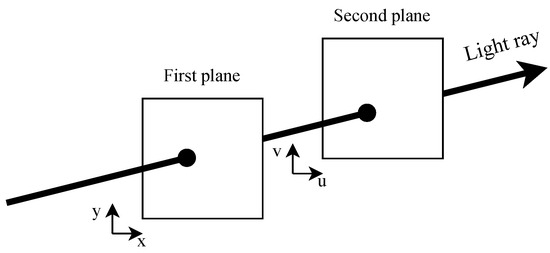
Figure 1. Two-plane parameterization for light field videos (LFVs).

An LFV captures spatial, angular, and temporal variations in light rays in contrast to a conventional 3-D video, which captures only spatial and temporal variations in light rays. This richness of information on LFVs leads to novel applications such as post-capture refocusing [5,6,7,8], depth estimation [9], and depth-velocity filtering [10], which are not possible with 3-D videos. Furthermore, LFVs are especially useful in augmented reality and virtual reality applications [11]. However, the data associated with an LFV are significantly larger compared to those of 3-D videos, e.g., one color channel of an LFV of size $8\times 8\times 434\times 625\times 16$ requires 2.17 GB, with 8 bits per pixel. This limits the potential of the real-time processing of LFVs, especially with mobile, edge, or web applications where storage is limited or the data rate is not sufficient for real-time communication. Therefore, to fully exploit the capabilities enabled by LFVs, efficient LFV compression techniques are required to be developed.

Several techniques have been proposed for the compression of four-dimensional (4-D) light fields and 5-D LFVs. Approaches proposed for light fields include methods based on the discrete cosine transform (DCT) [12], discrete wavelet transform (DWT) [13], and graph-based techniques [14]. However, their direct extension to 5-D LFVs often results in suboptimal performance due to the added temporal dimension and increased redundancy in data. Recent innovations, such as learning-based methods [15], and adaptations of existing video codecs [16], have shown promise for 5-D LFV compression but involve substantial computational overhead, limiting their practicality for real-time or resource-constrained scenarios.

In this paper, we propose a low-complexity LFV lossy compression technique using 5-D approximate discrete cosine transform (ADCT) algorithms. To the best of our knowledge, this is the first compression technique for LFVs using ADCT. Our key contributions are as follows:

• We introduce low-complexity ADCT algorithms for LFVs that approximate the type-II DCT, leveraging its excellent energy-compaction property, which is widely used in data compression applications. These ADCT algorithms significantly reduce computational complexity compared to the exact DCT.
• To further enhance the efficiency, we exploit the partial separability of LFV representations by considering blocks of size $8\times 8\times 8\times 8\times 8$ and applying 2-D $8\times 8$-point ADCT to SAIs of LFV frames with intra-view and inter-view configurations separately. We apply 2-D ADCT with respect to $(n_u,n_v)$ in the intra-view configuration and with respect to $(n_x,n_y)$ in the inter-view configuration, followed by a 1-D 8-point ADCT for the temporal dimension.
• We demonstrate that the proposed algorithm achieves over a 250-fold reduction in data volume with near-lossless fidelity (PSNR > 40 dB, SSIM > 0.9). Additionally, the computational complexity was significantly reduced, as the number of additions decreased from 56 to 14, and the number of multiplications was entirely eliminated (64 to 0) compared to the exact DCT.

The rest of this paper is organized as follows. In Section 2, we discuss the related work. We present a review of the DCT and ADCT in Section 3. In Section 4, we present the proposed LFV compression technique in detail. In Section 5, we present experimental results, and finally, in Section 6, we present the conclusion and future work.

2. Related Work

2.1. Light Field Compression

Light field compression techniques have evolved from traditional 2-D image compression methods, with the goal of extending these approaches to handle 4-D light fields. A key example is the JPEG Pleno verification model for lenslet light field compression, which illustrates how conventional methods can be adapted to the light field domain by partitioning the data into 4-D blocks and applying transforms such as the 4-D DCT [17]. However, while effective, this process is computationally intensive, which poses challenges for real-time applications. To reduce the computational complexity, various techniques have been developed. One such approach leverages the partial separability of light field representations by applying 2-D transforms sequentially, instead of all at once, to the 4-D blocks [18]. This reduces the overall processing load. Similarly, rearranging the SAIs of a light field along a third dimension to create 3-D blocks allows the use of the 3-D DCT, which offers a more manageable computational complexity [19]. Despite these optimizations, both techniques can struggle with more complex light field representations.

Beyond DCT-based approaches, the DWT has also been explored for light field compression, primarily to address the blocking artifacts commonly associated with DCT methods. The application of 4-D DWT has been shown to effectively reduce artifacts and improve compression efficiency [20]. JPEG2000 [13], which employs DWT, has inspired efforts to extend this method to light field compression, providing smoother reconstructions with fewer artifacts. Further advancements include the use of the Karhunen–Loève transform, which clusters micro-images into representative vectors for vector quantization. This technique has demonstrated superior performance in terms of the PSNR, particularly at lower bit rates, when compared to traditional methods [21]. Another promising direction is the graph Fourier transform, which models the light field’s color, disparity, and geometry information, reducing the number of transform coefficients by up to 21.92% while maintaining or improving the mean squared reconstruction error [14].

More recent innovations in light field compression have introduced pre-demosaic graph-based techniques. These approaches bypass the demosaicking stage to reduce data redundancy, improving coding performance for high-quality archival applications. Techniques such as graph-based lifting transforms and optimized intra-prediction have proven particularly effective for improving compression efficiency [22]. Additionally, graph learning and dictionary-guided sparse coding methods have shown significant improvements in bit rate reduction and PSNR, particularly by encoding key views and reconstructing other views using learned graph adjacency matrices [23]. Due to these advancements, the spatial–angular decorrelation network has demonstrated how convolution-based techniques can jointly compress spatial and angular information, resulting in up to 79.6% bit rate reduction while preserving high geometric consistency in light fields [24]. In parallel, methods like the macro-view image technique group 3 × 3 light field views to improve both compression efficiency and random access. Using the central view as a reference, this approach reduces the decoding latency and facilitates parallel processing [25].

Recent developments in the JPEG Pleno framework have also contributed to improved light field compression. These include replacing sample-based forward warping with mesh-based backward warping, which enhances view prediction accuracy and interpolation [26]. Additionally, the introduction of the breakpoint-dependent DWT has further enhanced the rate-distortion performance for coding depth maps. Another key innovation, the slanted 4D-DCT coding mode, applies an adaptive geometric transformation before the 4-D DCT, achieving an over 31% BD-rate reduction across various light field types [27].

2.2. Light Field Video Compression

Compared to the methods proposed for light field compression, a few methods have been proposed for LFV compression. In [15], a deep learning-based framework was proposed for LFV compression that effectively leverages the geometric structure of LFVs. This approach combines a sparse coding strategy with convolutional neural network-based view synthesis to reduce the number of encoded views while reconstructing the remaining ones through learned synthesis algorithms. By introducing adaptive prediction structures and synthesized candidate reference-based inter-frame prediction, they significantly reduce inter-view and inter-frame redundancies. The method achieves considerable bitrate savings compared to traditional multi-view video coding methods like HEVC, demonstrating the potential of learning-based compression techniques for LFVs. Building on the need for efficient LFV compression, in [16], a method previously applied to 4-D light fields was extended into the 5-D domain by incorporating the time dimension into the compression process. This approach transforms multi-view videos into multi-focus images and rearranges them in the time domain for efficient compression using standard video codecs such as HEVC. This rearrangement allows both spatial and temporal redundancies to be exploited, improving compression efficiency. Through experiments with synthetic videos, the proposed method outperforms HEVC when applied directly to LFVs, especially at low bit rates, making it highly suitable for bandwidth-constrained applications. Similarly, in [28], the authors address the unique characteristics of raw plenoptic LFV data by introducing a novel motion vector resolution based on hexagonal lattice resolution. This resolution is optimized for the micro-image structure of plenoptic videos, where motion vectors naturally align with a hexagonal pattern. Using the hexagonal lattice resolution within the VVC codec, the authors demonstrate substantial improvements in rate-distortion performance compared to conventional integer-pel and half-pel resolutions. While the quarter-pel resolution remains competitive in some cases, the hexagonal lattice resolution provides a fresh approach for optimizing motion vector prediction, making it a promising advancement for LFV compression.

In contrast, our method not only focuses on achieving high compression ratios but also prioritizes computational efficiency. To address these dual objectives, we employ ADCT, which offers a fundamentally different approach to LFV compression by significantly reducing computational complexity without sacrificing compression efficiency. ADCT algorithms furnish approximations to the exact DCT by replacing floating-point operations with simplified arithmetic operations, such as additions and shifts [29,30,31,32,33]. This low-complexity nature makes ADCT particularly well suited for real-time and resource-constrained scenarios, avoiding the computational overhead associated with learning-based methods or traditional codecs [18]. Furthermore, ADCT’s excellent energy compaction properties enable it to efficiently manage the high dimensionality of LFV data. It effectively exploits redundancies across spatial, angular, and temporal dimensions, making it a scalable and robust solution. By addressing challenges that existing methods only partially resolve, ADCT bridges the gap between performance and practicality in LFV compression. The following subsection delves deeper into the ADCT algorithms currently available and their relevance to this work.

2.3. Approximate Discrete Cosine Transform

The DCT is a widely used transform for image and video compression, for example, in standards such as JPEG [34], MPEG-1 [35], and H.264 [36]. DCT is known for its good energy compaction properties. Several ADCT methods have been proposed to reduce the arithmetic operations of DCT. These methods focus on reducing arithmetic operations without significantly compromising the transform’s performance. The ADCT methods proposed in the literature include the 8-point DCT [29,30,31,32,33] and the 16-point DCT [37]. These approximations often involve transforming the original DCT matrix into a product of simpler matrices, typically comprising a diagonal matrix with non-trivial multiplicands and another matrix with trivial multiplicands, such as small powers of two [33]. By replacing floating-point operations with simpler arithmetic, these ADCT techniques significantly reduce computational complexity, making them suitable for real-time compression tasks, while still maintaining an acceptable level of compression efficiency. The arithmetic complexity of several ADCT algorithms is summarized in Table 1.

Table 1. Arithmetic complexity of various DCT methods.

DCT Method	Mult	Add	Shifts	Total
Exact DCT	64	56	0	120
BAS2008 [29]	0	18	2	20
BAS2011 [30] with $a=0$	0	16	0	16
BAS2011 [30] with $a=1$	0	18	0	18
CB2011 [31]	0	22	0	22
Modified CB2011 [32]	0	14	0	14
PMC2014 [33]	0	14	0	14

3. Review of DCT and ADCT

3.1. 1-D DCT

Let $\mathbf{x}$ be an N-point vector, whose entries are given by $x\left[n\right]$ for $n=0,1,\dots ,N-1$, and $\mathbf{y}$ is the 1-D DCT transformation of $\mathbf{x}$, whose entries are given by [38]

$$y\left[k\right]=a\left[k\right]·\sum _{n=0}^{N-1}x\left[n\right]·cos\left({\displaystyle \frac{\pi k(2n+1)}{2N}}\right),$$

(1)

where

$$a\left[k\right]={\displaystyle \frac{1}{\sqrt{N}}}\left\{\begin{array}{cc}1,\hfill & k=0,\hfill \\ \sqrt{2},\hfill & k=1,2,\dots ,N-1.\hfill \end{array}\right.$$

(2)

Approximation derivation and algorithm development take advantage of matrix formalism. Thus, (1) is written as

$$\mathbf{y}={\mathbf{C}}_N·\mathbf{x},$$

(3)

where ${\mathbf{C}}_N$ is the DCT matrix whose entries are given by $c_{k,n}=a\left[k\right]·cos\left({\displaystyle \frac{\pi k(2n+1)}{2N}}\right)$, $k,n=0,1,\dots ,N-1$. To reduce arithmetic complexity, instead of the exact DCT matrix ${\mathbf{C}}_N$, an approximate DCT matrix ${\widehat{\mathbf{C}}}_N$ is used, which can be written as [31,32,33]

$${\widehat{\mathbf{C}}}_N={\mathbf{S}}_N·{\mathbf{T}}_N,$$

(4)

where ${\mathbf{S}}_N$ is a diagonal matrix that normalizes the energy of the basis vector, and ${\mathbf{T}}_N$ is a low-complexity matrix of trivial multiplicands.

3.2. 2-D DCT

Let $\mathbf{X}$ be an $N\times N$ matrix, whose entries are given by $x[n_1,n_2]$ for $n_1,n_2=0,1,\dots ,N-1$, and $\mathbf{Y}$ is the 2-D DCT transformation of $\mathbf{X}$, whose entries are given by [39]

$$\begin{array}{cc}\hfill y[k_1,k_2]=& a\left[k_1\right]·a\left[k_2\right]·\sum _{n_1=0}^{N-1}\sum _{n_2=0}^{N-1}x[n_1,n_2]·\hfill \\ \hfill & cos\left({\displaystyle \frac{\pi k_1(2n_1+1)}{2N}}\right)·cos\left({\displaystyle \frac{\pi k_2(2n_2+1)}{2N}}\right).\hfill \end{array}$$

(5)

Under matrix formalism, the above definition is equivalent to the following expression:

$$\mathbf{Y}={\mathbf{C}}_N·\mathbf{X}·{\mathbf{C}}_N^T.$$

(6)

For the 2-D approximate DCT, it suffices to employ a given approximation ${\widehat{\mathbf{C}}}_N$ instead of the exact DCT matrix ${\mathbf{C}}_N$ in (6).

4. Proposed 5-D ADCT-Based LFV Compression Method

The proposed method uses ADCT algorithms, as shown in Figure 2, to achieve low computational complexity while maintaining high compression efficiency. Unlike exact DCT, ADCT algorithms significantly reduce arithmetic complexity, making the method well suited for real-time processing and resource-constrained environments. Furthermore, the method efficiently processes LFVs by applying transformations along spatial, angular, and temporal dimensions sequentially. Using ADCT algorithms [33], which approximate a type II DCT, the proposed method achieves efficient compression through reduced arithmetic operations, such as 14 additions, making it particularly suitable for real-time applications. The partial separability of the 5-D representation enables independent processing in intra-view, inter-view, and temporal domains, avoiding computationally intensive joint 5-D transformations.

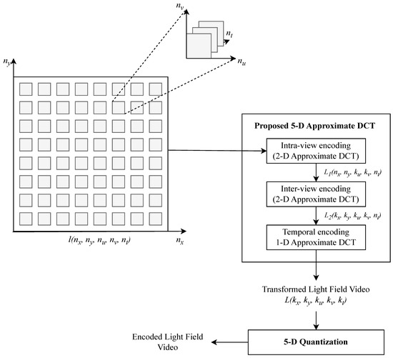
Figure 2. Overview of the proposed 5-D ADCT-based LFV compression. An LFV is processed in three steps: (1) intra-view using 2-D ADCT, with respect to $(n_u,n_v)$, (2) inter-view using 2-D ADCT, with respect to $(n_x,n_y)$, and (3) temporal using 1-D ADCT, with respect to $n_t$.

The proposed 5-D ADCT-based LFV compression method processes LFV data in four sequential steps: intra-view encoding, inter-view encoding, temporal encoding, and quantization. Each step is detailed below:

Step 1—Intra-view Encoding: The input to the system, denoted as $l(n_x,n_y,n_u,n_v,n_t)$, represents a 5-D LFV signal with size $(N_x\times N_y\times N_u\times N_v\times N_t)$ samples, where $N_t$ is the number of frames, $N_x\times N_y$ is the number of SAIs per frame, and each SAI has a resolution of $N_u\times N_v$ pixels. Intra-view encoding transforms the spatial domain within each SAI. All SAIs of each frame are partitioned into $8\times 8$ pixel blocks, and 2-D ADCT is applied to each block. This step creates the mixed domain signal $L_1(n_x,n_y,k_u,k_v,n_t)$, which represents the spatial ADCT components for each intra-view. The process is illustrated in Figure 3.

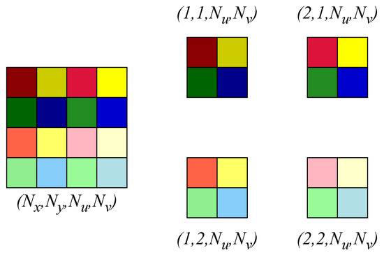
Figure 3. Overview of the intra-view encoding process applied to the LFV signal. Each SAI of $N_u\times N_v$ pixels within the frame is partitioned into $2\times 2$ pixel blocks, followed by the application of 2-D ADCT to transform the spatial domain into the spatial frequency domain, resulting in the mixed domain signal $L_1(n_x,n_y,k_u,k_v,n_t)$. Note that, for illustration, we consider $N_u=N_v=4$ and $2\times 2$ pixel blocks instead of $8\times 8$ pixel blocks.

Step 2—Inter-view Encoding: After intra-view encoding, inter-view encoding processes angular redundancies across SAIs. From $L_1(n_x,n_y,k_u,k_v,n_t)$, $N_x\times N_y$ viewpoint blocks are created by reorganizing pixels across SAIs in each LFV frame. These are further partitioned into $8\times 8$ blocks, and 2-D ADCT is applied to capture angular correlations. The output of this step is a new mixed domain signal $L_2(k_x,k_y,k_u,k_v,n_t)$, which incorporates both spatial and angular ADCT components. This transformation is shown in Figure 4.

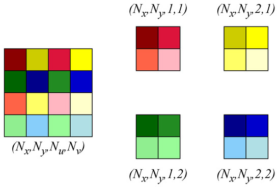
Figure 4. Overview of the inter-view encoding process. Angular redundancies across SAIs are processed by reorganizing $N_x\times N_y$ viewpoint blocks within each LFV frame. These blocks are partitioned into $2\times 2$ pixel groups, and 2-D ADCT is applied to extract angular correlations. The resulting mixed domain signal $L_2(k_x,k_y,k_u,k_v,n_t)$ combines both spatial and angular ADCT components. Note that, for illustration, we consider $N_x=N_y=4$ and $2\times 2$ pixel blocks instead of $8\times 8$ pixel blocks.

Step 3—Temporal Encoding: Temporal encoding addresses redundancies along the time dimension. For each pixel and viewpoint in $L_2(k_x,k_y,k_u,k_v,n_t)$, 1-D ADCT is applied to vectors of size $8\times 1$ along the time axis $n_t$. This transformation produces the fully transformed 5-D signal $L(k_x,k_y,k_u,k_v,k_t)$, which compactly represents spatial, angular, and temporal information. Figure 5 illustrates this process.

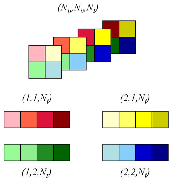
Figure 5. Overview of the temporal encoding process. Temporal redundancies along the time dimension are addressed by applying 1-D ADCT to vectors of size $4\times 1$ along the $n_t$ axis for each pixel and view point in $L_2(k_x,k_y,k_u,k_v,n_t)$. This process results in the fully transformed 5-D signal $L(k_x,k_y,k_u,k_v,k_t)$, which compactly integrates spatial, angular, and temporal information. Note that, for illustration, we consider $N_t=4$ and $4\times 1$ pixel blocks instead of $8\times 1$ pixel blocks.

Step 4—Quantization: Finally, $L(k_x,k_y,k_u,k_v,k_t)$ is quantized to compress the LFV. The signal $L(k_x,k_y,k_u,k_v,k_t)$ is partitioned into $8\times 8\times 8\times 8\times 8$ blocks, and quantization is applied to each block as described in [34]:

$$\begin{array}{c}\hfill L_q\left(\mathbf{k}\right)=round\left({\displaystyle \frac{L\left(\mathbf{k}\right)}{Q\left(\mathbf{k}\right)}}\right),\end{array}$$

(7)

where $\mathbf{k}=(k_x,k_y,k_u,k_v,k_t)$, $round(·)$ represents element-wise rounding, $Q\left(\mathbf{k}\right)$ is the 5-D quantization matrix with constant entries and division is performed element-wise. After quantization, only the nonzero coefficients are retained in $L_q\left(\mathbf{k}\right)$, resulting in a compressed representation of the LFV.

During decompression, the signal is reconstructed using the retained coefficients. The decompressed signal $L_{dc}\left(\mathbf{k}\right)$ is obtained as

$$\begin{array}{c}\hfill L_{dc}\left(\mathbf{k}\right)=L_q\left(\mathbf{k}\right)·Q\left(\mathbf{k}\right),\end{array}$$

(8)

where multiplication is applied element-wise. This quantization and reconstruction process ensures effective compression by discarding less significant coefficients while retaining critical information for accurate decompression.

This sequential processing method exploits the partial separability of LFV, efficiently reducing computational complexity while preserving essential spatial, angular, and temporal correlations for effective 5-D compression.

5. Experimental Results

5.1. Dataset

This paper evaluates the performance of LFV compression using three publicly available standard LFVs: Car, David, and Toys [40]. These LFVs represent diverse real-world scenarios. The Car LFV features a dynamic scene where a car moves from right to left at a constant speed, with a resolution of $512\times 352$, making it ideal for testing the method’s capability to handle high motion and temporal changes. The David LFV consists of a single sculpture on a turntable against a green background, with a resolution of $480\times 320$. The Toys LFV includes two toys on a turntable with a green background, offering moderate complexity and structured motion, with a resolution of $480\times 320$. All three LFVs were generated from a $15\times 15$ multiple-camera array. For experiments, $8\times 8$ views are considered, and all SAIs are in YUV420 format. Table 2 summarizes the size and the minimum and maximum values of each channel of the LFVs. The diversity of these LFVs ensures a robust evaluation of the proposed ADCT-based compression method, as they represent varying levels of motion, angular complexity, and real-world scenarios. The results, discussed in this section, confirm the method’s effectiveness across these diverse cases, with slight variations noted for high-motion scenes, further affirming its generalizability and robustness.

Table 2. Specifications of LFVs employed for experiments.

LFV	Channel	Size	Min	Max
Car	U	$8\times 8\times 176\times 256\times 24$	25	181
	V	$8\times 8\times 176\times 256\times 24$	80	193
	Y	$8\times 8\times 352\times 512\times 24$	3	255
David	U	$8\times 8\times 160\times 240\times 24$	49	122
	V	$8\times 8\times 160\times 240\times 24$	107	151
	Y	$8\times 8\times 320\times 480\times 24$	43	229
Toy	U	$8\times 8\times 160\times 240\times 24$	3	160
	V	$8\times 8\times 160\times 240\times 24$	50	224
	Y	$8\times 8\times 320\times 480\times 24$	12	255

5.2. Evaluation Metrics

Compression quality is measured by means of the PSNR and the SSIM index, and both are applied to each SAI of the decompressed LFVs with the original uncompressed LFVs as the reference (ground truth) [41]. The PSNR between the original SAI A and the reconstructed SAI A′ is computed as [41]

$$PSNR=20{log}_{10}\left({\displaystyle \frac{2^N-1}{\sqrt{MSE}}}\right),$$

(9)

where $N=8$ is the number of bits employed to represent an LFV, and the $MSE$ between the two $M\times N$ SAIs $\mathbf{A}$ and $\mathbf{A}\prime$ is given by

$$MSE={\displaystyle \frac{1}{MN}}\sum _{i=0}^{M-1}\sum _{j=0}^{N-1}{(\mathbf{A}(i,j)-{\mathbf{A}}^{\prime }(i,j))}^2.$$

(10)

The SSIM for A and A′s is given by [42]

$$SSIM={\displaystyle \frac{(2{\mu }_A{\mu }_{A^{\prime }}+C_1)(2{\sigma }_{A{A}^{\prime }}+C_2)}{({\mu }_A^2+{\mu }_{A^{\prime }}^2+C_1)({\sigma }_A^2+{\sigma }_{A^{\prime }}^2+C_2)}},$$

(11)

where ${\mu }_A,{\mu }_{A^{\prime }},{\sigma }_A,{\sigma }_{A^{\prime }}$, and ${\sigma }_{A{A}^{\prime }}$ are the local means, standard deviations, and cross-covariance for SAIs $\mathbf{A}$ and ${\mathbf{A}}^{\prime }$, respectively, and $C_1$ and $C_2$ are constants used to avoid numerical instability [42].

The PSNR and SSIM for LFVs are computed by averaging the PSNRs and SSIMs of SAIs individually. The final $SSI{M}_{YCbCr}$ of the entire LFV is computed using only the luminance component (Y) [41]. The final PSNR, $PSN{R}_{YCbCr}$, of an entire LFV is computed using the PSNR of the luminance component ($PSN{R}_Y$) and the PSNRs of the blue- and red-difference chroma components ($PSN{R}_{Cb}$ and $PSN{R}_{Cr}$) as [41]

$$\begin{array}{c}\hfill PSN{R}_{YCbCr}={\displaystyle \frac{6PSN{R}_Y+PSN{R}_{Cb}+PSN{R}_{Cr}}{8}}.\end{array}$$

(12)

Another metric for evaluating the proposed algorithm is the computational complexity, which we assess in terms of the number of arithmetic operations. For example, for an LFV with size $(N_x\times N_y\times N_u\times N_v\times N_t)$ samples, the algorithm performs the following operations: (1) $N_x\times N_y\times {\displaystyle \frac{N_u}{8}}\times {\displaystyle \frac{N_v}{8}}\times N_t$ 2-D DCT operations (2) ${\displaystyle \frac{N_x}{8}}\times {\displaystyle \frac{N_y}{8}}\times N_u\times N_v\times N_t$ 2-D DCT operations, and (3) $N_x\times N_y\times N_u\times N_v\times {\displaystyle \frac{N_t}{8}}$ 1-D DCT operations. The number of arithmetic operations in the DCT operations largely determines the algorithm’s overall complexity. As shown in Table 1, if the exact DCT algorithm is used, the 1-D DCT requires 64 multiplications and 56 additions. However, the PMC2014 ADCT algorithm [33] reduces the number of additions to just 14 and eliminates multiplications entirely for the 1-D DCT operation, leading to a more than 10 times reduction of arithmetic complexity [33]

5.3. Results and Discussion

The proposed 5-D ADCT LFV compression attempts to exploit the redundancy in both the intra-view and inter-view of an LFV. In Figure 6, we demonstrate this by comparing the proposed 5-D ADCT-based compression with intra-view and temporal-only 3-D ADCT-based compression and inter-view and temporal-only 3-D ADCT-based compression. Here, we employ the ADCT algorithms proposed in [33]. We observe that the inter-view and temporal-only 3-D ADCT achieves better compression than intra-view and temporal-only 3-D ADCT, because the pixels in an $8\times 8$ block in inter-view (which represents light emanating from the same point in a scene with different directions) have higher correlation compared to those in intra-view (which represents light emanating from the neighboring points in a scene in the same direction). More importantly, 5-D ADCT-based compression shows the best performance in terms of both the PSNR and SSIM as it utilizes redundancy in both intra-veiw and inter-view. In Table 3, we present the variation in the PSNR and SSIM with different quantization for the Y channel of the LFV David. The lowest bits per pixel achieved is $0.03$ when the quantization value is greater than or equal to 80. For these bits per pixel value, the PSNR is about 45 dB and the SSIM is $0.95$. We note that each color channel is represented with 8 bits for a pixel, and $0.03$ bits per pixel results in approximately 266 times compression. To further visually confirm the effectiveness of the proposed LFv compression method, we present the SAIs (corresponding to $N_x=N_y=4$) of the Car LFV at the frame 35, 40, and 45 with three different quantization values $q=1$, $q=10$, and $q=200$ in Figure 7. The reconstructed (or decompressed) frames with $q=1$ and $q=10$ are almost the same as the ground truth, whereas the decompressed frames with $q=200$ have slightly lower intensity. This confirms that the proposed LFV compression leads high-fidelity reconstructed LFVs even with higher compression rates.

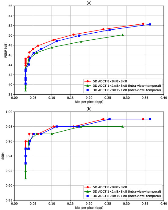
Figure 6. (a) PSNR vs. bits per pixel (b) SSIM vs. bits per pixel for 5-D ADCT, intra-view + temporal only 3-D DCT and inter-view + temporal only 3-D DCT. Here, the ADCT algorithm proposed in [33] is employed.

Table 3. Variation in the PSNR and the SSIM with different quantization values.

Quantization Value	Bits per Pixel [bpp]	PSNR [dB]	SSIM	Energy Retained
1	1.33	62.32	1.00	1.00
3	0.47	55.26	0.99	1.00
5	0.28	53.53	0.99	1.00
7	0.20	52.41	0.99	1.00
10	0.14	51.26	0.99	0.99
15	0.09	50.06	0.98	0.99
25	0.06	48.76	0.98	0.98
35	0.04	48.06	0.97	0.97
50	0.04	47.44	0.97	0.96
80	0.03	46.67	0.97	0.95
100	0.03	46.31	0.97	0.95
120	0.03	45.97	0.96	0.95
150	0.03	45.65	0.96	0.94
180	0.03	45.25	0.96	0.94
200	0.03	44.99	0.96	0.94

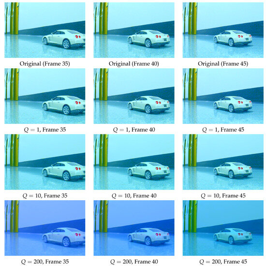
Figure 7. The SAIs ($N_x=N_y=4$) of the Car LFV at frames 35, 40, and 45. The first row shows the original images, while the second, third, and fourth rows display the reconstructed images at quantization values of $Q=1$, $Q=10$, and $Q=200$, respectively.

In Figure 8, the PSNR achieved for different compression levels (bits per pixel) are shown for six ADCT algorithms and the exact DCT. When decreasing bits per pixel, i.e., higher compression, the PSNR also decreases for the three LFVs considered in the experiments. All PSNR vs. bits per pixel graphs nearly follow the same characteristics for the three LFVs. For LFVs Car and Toy, the PSNR converges to approximately 41 dB at bits per pixel near to 0.04, as the lower value. For LFV David, the PSNR converges approximately to 45 dB at bits per pixel near 0.03. As mentioned in Table 2, LFV David has a narrower range compared to the other two LFVs. This may be the reason for better PSNR values for smaller bits per pixel values. In Figure 9, the variation in SSIM with respect to bits per pixel. The SSIM is typically decreased with the increased compression. Similarly to the PSNR, the SSIM is also slightly better for LFV David, compared to the Car and Toy LFVs. In comparing the different ADCT methods, on one hand, the ADCT proposed in [31] provides the best PSNR and SSIM for all three LFVs though the number of arithmetic operations is relatively higher compared to other ADCT approaches considered in the experiments. On the other hand, the ADCT methods that required the lowest arithmetic operations, Modified CB-2011 [32] and PMC 2014 [33], provide comparable performance with respect to the SSIM for most of the other ADCT methods even though the performance with respect to the PSNR is slightly lower compared to other ADCT methods. Overall, we observe that ADCT results in a slight degradation in the quality of the reconstructed LFVs, in terms of the PSNR and SSIM, compared to the exact DCT; however, the reduction in arithmetic operations is significant with the ADCTs compared to the exact DCT, e.g., more than a 10 times reduction with the Modified CB-2011 [32] and PMC 2014 [33] methods.

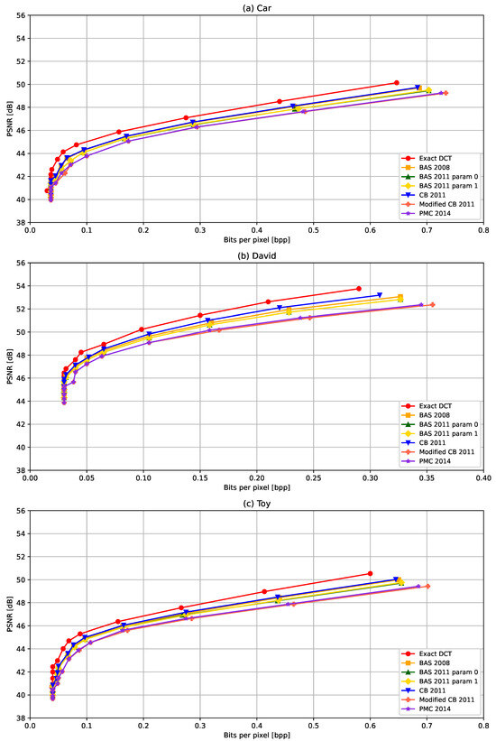
Figure 8. PSNR with respect to bits per pixel with different ADCT algorithms: BAS-2008 [29], BAS-2011 for parameter 0 [30], BAS-2011 for parameter 1 [30], CB-2011 [31], Modified CB-2011 [32], and PMC 2014 [33], and the exact DCT in the 5-D domain for LFVs (a) Car, (b) David, and (c) Toy.

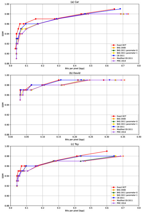
Figure 9. SSIM with respect to bits per pixel with different ADCT algorithms: BAS-2008 [29], BAS-2011 for parameter 0 [30], BAS-2011 for parameter 1 [30], CB-2011 [31], Modified CB-2011 [32] PMC 2014 [33], and the exact DCT in 5-D domain for LFVs (a) Car, (b) David, and (c) Toy.

To verify the high fidelity of the reconstructed LFVs, after compressing LFVs with the proposed method, we analyze epi-polar plane images. Note that epi-polar plane images represent depth and angular information LFVs, and have a structure of straight lines of which gradients depend on the depth [4,7]. Figure 10 shows the epi-polar plane images from frame 40 of the original LFV and the reconstructed LFV at quantization value 200. We observe that the straight-line structure is mostly preserved in the reconstructed frame. This visual comparison demonstrates that angular continuity and depth fidelity are maintained even with this higher compression rate. To further verify, the PSNR and SSIM values, computed as the average over 10 frames, are computed for the epi-polar plane images for five quantization levels, which are shown in Table 4. We observe that the PSNR values are greater than 65 dB, while the SSIM values are greater than 0.804. These values confirm that the proposed algorithm preserves the angular and depth information with very high fidelity.

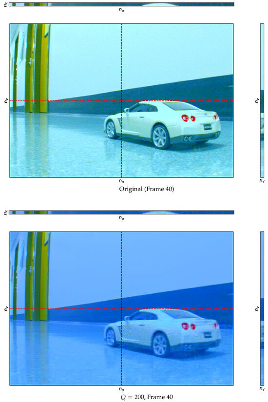
Figure 10. Epi-polar images of the original (top row) and reconstructed (bottom row) Car LFV at frame 40 with the quantization value $Q=200$. Note that the straight-line structure of the epi-polar plane images is preserved in the reconstructed LFV.

Table 4. PSNR and SSIM values with different quantization values for horizontal and vertical epi-polar plane images.

val	PSNR (dB)		SSIM
	Horizontal	Vertical	Horizontal	Vertical
1	101.045	97.640	1.000	1.000
5	88.922	84.948	0.961	0.965
10	83.747	79.816	0.910	0.937
50	73.567	69.676	0.835	0.875
200	71.285	65.883	0.804	0.831

6. Conclusions and Future Work

LFVs are widely used in different applications, but due to a large amount of data, the potential of the real-time processing of LFVs is limited. A low-complexity compression approach is proposed for 5-D LFVs using multiplier-less 5-D ADCT. To reduce complexity further, we employ partial separability, and 5-D compression is performed in the following order: 2-D intra-view compression, 2-D inter-view compression, and temporal compression. The effectiveness of the proposed 5-D ADCT-based compression, compared to 2-D inter-view + 1-D temporal only and 2-D intra-view + 1-D temporal only ADCT compression, was verified using simulations. For the three LFVs considered, PSNRs greater than 41 dB and SSIM indices greater than 0.9 were achieved at 0.03 bits per pixel, i.e., more than 250 times compression. Future work includes the implementation of the proposed LFV compression algorithm in hardware such as a field-programmable gate array to achieve the real-time or near real-time compression of LFVs.

References

- Adelson, E.H.; Bergen, J.R. The Plenoptic Function and the Elements of Early Vision; Vision and Modeling Group, Media Laboratory, Massachusetts Institute of Technology: Cambridge, MA, USA, 1991; Volume 2. [Google Scholar]
- Zhang, C.; Chen, T. A survey on image-based rendering—Representation, sampling and compression. Signal Process. Image Commun. 2004, 19, 1–28. [Google Scholar] [CrossRef]
- Shum, H.Y.; Kang, S.B.; Chan, S.C. Survey of image-based representations and compression techniques. IEEE Trans. Circuits Syst. Video Technol. 2003, 13, 1020–1037. [Google Scholar] [CrossRef]
- Levoy, M.; Hanrahan, P. Light field rendering. In Seminal Graphics Papers: Pushing the Boundaries, Volume 2; Association for Computing Machinery: New York, NY, USA, 1996; pp. 441–452, Conference: SIGGRAPH’96: 23rd International Conference on Computer Graphics and Interactive Techniques; ISBN 978-0-89791-746-9. [Google Scholar]
- Ng, R.; Levoy, M.; Brédif, M.; Duval, G.; Horowitz, M.; Hanrahan, P. Light Field Photography with a Hand-Held Plenoptic Camera. Ph.D. Thesis, Stanford University, Stanford, CA, USA, 2005. [Google Scholar]
- Fiss, J.; Curless, B.; Szeliski, R. Refocusing plenoptic images using depth-adaptive splatting. In Proceedings of the 2014 IEEE International Conference on Computational Photography (ICCP), Santa Clara, CA, USA, 2–4 May 2014; pp. 1–9. [Google Scholar]
- Dansereau, D.G.; Pizarro, O.; Williams, S.B. Linear volumetric focus for light field cameras. ACM Trans. Graph. 2015, 34, 15:1–15:20. [Google Scholar] [CrossRef]
- Jayaweera, S.S.; Edussooriya, C.U.; Wijenayake, C.; Agathoklis, P.; Bruton, L.T. Multi-volumetric refocusing of light fields. IEEE Signal Process. Lett. 2020, 28, 31–35. [Google Scholar] [CrossRef]
- Kinoshita, T.; Ono, S. Depth estimation from 4D light field videos. In Proceedings of the International Workshop on Advanced Imaging Technology (IWAIT) 2021, Online, 5–6 January 2021; International Society for Optics and Photonics (SPIE): Bellingham, WA, USA, 2021; Volume 11766, p. 117660A. [Google Scholar]
- Edussooriya, C.U.; Dansereau, D.G.; Bruton, L.T.; Agathoklis, P. Five-dimensional depth-velocity filtering for enhancing moving objects in light field videos. IEEE Trans. Signal Process. 2015, 63, 2151–2163. [Google Scholar] [CrossRef]
- Wang, J.; Xiao, X.; Hua, H.; Javidi, B. Augmented reality 3D displays with micro integral imaging. J. Disp. Technol. 2015, 11, 889–893. [Google Scholar] [CrossRef]
- Conti, C.; Soares, L.D.; Nunes, P. Dense light field coding: A survey. IEEE Access 2020, 8, 49244–49284. [Google Scholar] [CrossRef]
- Rabbani, M.; Joshi, R. An overview of the JPEG 2000 still image compression standard. Signal Process. Image Commun. 2002, 17, 3–48. [Google Scholar] [CrossRef]
- Elias, V.R.M.; Martins, W.A. On the use of graph Fourier transform for light-field compression. J. Commun. Inf. Syst. 2018, 33. [Google Scholar] [CrossRef]
- Wang, B.; Xiang, W.; Wang, E.; Peng, Q.; Gao, P.; Wu, X. Learning-based high-efficiency compression framework for light field videos. Multimed. Tools Appl. 2022, 81, 7527–7560. [Google Scholar] [CrossRef]
- Umebayashi, S.; Kodama, K.; Hamamoto, T. Study on 5-D light field compression using multi-focus images. In Proceedings of the International Workshop on Advanced Imaging Technology (IWAIT) 2022, Hong Kong, China, 4–6 January 2022; International Society for Optics and Photonics (SPIE): Bellingham, WA, USA, 2022; Volume 12177, Article 121770R. pp. 137–142. [Google Scholar] [CrossRef]
- Alves, G.D.O.; De Carvalho, M.B.; Pagliari, C.L.; Freitas, P.G.; Seidel, I.; Pereira, M.P.; Vieira, C.F.S.; Testoni, V.; Pereira, F.; Da Silva, E.A. The JPEG Pleno light field coding standard 4D-transform mode: How to design an efficient 4D-native codec. IEEE Access 2020, 8, 170807–170829. [Google Scholar] [CrossRef]
- Liyanage, N.; Wijenayake, C.; Edussooriya, C.U.; Madanayake, A.; Cintra, R.J.; Ambikairajah, E. Low-complexity real-time light field compression using 4-D approximate DCT. In Proceedings of the 2020 IEEE International Symposium on Circuits and Systems (ISCAS), Seville, Spain, 12–14 October 2020; IEEE: Piscataway, NJ, USA, 2020; pp. 1–5. [Google Scholar]
- Mehanna, A.; Aggoun, A.; Abdulfatah, O.; Swash, M.R.; Tsekleves, E. Adaptive 3D-DCT based compression algorithms for integral images. In Proceedings of the 2013 IEEE International Symposium on Broadband Multimedia Systems and Broadcasting (BMSB), London, UK, 5–7 June 2013; IEEE: Piscataway, NJ, USA, 2013; pp. 1–5. [Google Scholar]
- Kuo, C.L.; Lin, Y.Y.; Lu, Y.C. Analysis and implementation of Discrete Wavelet Transform for compressing four-dimensional light field data. In Proceedings of the 2013 IEEE International SOC Conference, Erlangen, Germany, 4–6 September 2013; IEEE: Piscataway, NJ, USA, 2013; pp. 134–138. [Google Scholar]
- Jang, J.S.; Yeom, S.; Javidi, B. Compression of ray information in three-dimensional integral imaging. Opt. Eng. 2006, 44, 127001. [Google Scholar] [CrossRef]
- Chao, Y.H.; Hong, H.; Cheung, G.; Ortega, A. Pre-demosaic graph-based light field image compression. IEEE Trans. Image Process. 2022, 31, 1816–1829. [Google Scholar] [CrossRef]
- Zhang, Y.; Dai, W.; Li, Y.; Li, C.; Hou, J.; Zou, J.; Xiong, H. Light field compression with graph learning and dictionary-guided sparse coding. IEEE Trans. Multimed. 2022, 25, 3059–3072. [Google Scholar] [CrossRef]
- Tong, K.; Jin, X.; Wang, C.; Jiang, F. SADN: Learned light field image compression with spatial-angular decorrelation. In Proceedings of the ICASSP 2022–2022 IEEE International Conference on Acoustics, Speech and Signal Processing (ICASSP), Singapore, 23–27 May 2022; IEEE: Piscataway, NJ, USA, 2022; pp. 1870–1874. [Google Scholar]
- Amirpour, H.; Pinheiro, A.; Pereira, M.; Lopes, F.J.; Ghanbari, M. Efficient light field image compression with enhanced random access. ACM Trans. Multimed. Comput. Commun. Appl. (TOMM) 2022, 18, 1–18. [Google Scholar] [CrossRef]
- Li, Y.; Mathew, R.; Taubman, D. JPEG Pleno Light Field Encoder with Mesh based View Warping. In Proceedings of the 2023 IEEE International Conference on Image Processing (ICIP), Kuala Lumpur, Malaysia, 8–11 October 2023; IEEE: Piscataway, NJ, USA, 2023; pp. 2100–2104. [Google Scholar]
- De Carvalho, M.B.; Pagliari, C.L.; de OE Alves, G.; Schretter, C.; Schelkens, P.; Pereira, F.; Da Silva, E.A. Supporting Wider Baseline Light Fields in JPEG Pleno With a Novel Slanted 4D-DCT Coding Mode. IEEE Access 2023, 11, 28294–28317. [Google Scholar] [CrossRef]
- Huu, T.N.; Van, V.D.; Yim, J.; Jeon, B. Raw Plenoptic Video Coding Under Hexagonal Lattice Resolution of Motion Vectors. In Proceedings of the ICASSP 2022—2022 IEEE International Conference on Acoustics, Speech and Signal Processing (ICASSP), Singapore, 23–27 May 2022; IEEE: Piscataway, NJ, USA, 2022; pp. 1621–1624. [Google Scholar]
- Bouguezel, S.; Ahmad, M.O.; Swamy, M. Low-complexity 8 × 8 transform for image compression. Electron. Lett. 2008, 44, 1249–1250. [Google Scholar] [CrossRef]
- Bouguezel, S.; Ahmad, M.O.; Swamy, M. A low-complexity parametric transform for image compression. In Proceedings of the 2011 IEEE International Symposium of Circuits and Systems (ISCAS), Rio de Janeiro, Brazil, 15–18 May 2011; IEEE: Piscataway, NJ, USA, 2011; pp. 2145–2148. [Google Scholar]
- Cintra, R.J.; Bayer, F.M. A DCT approximation for image compression. IEEE Signal Process. Lett. 2011, 18, 579–582. [Google Scholar] [CrossRef]
- Bayer, F.M.; Cintra, R.J. DCT-like transform for image compression requires 14 additions only. Electron. Lett. 2012, 48, 919–921. [Google Scholar] [CrossRef]
- Potluri, U.S.; Madanayake, A.; Cintra, R.J.; Bayer, F.M.; Kulasekera, S.; Edirisuriya, A. Improved 8-point approximate DCT for image and video compression requiring only 14 additions. IEEE Trans. Circuits Syst. I Regul. Pap. 2014, 61, 1727–1740. [Google Scholar] [CrossRef]
- Pennebaker, W.B.; Mitchell, J.L. JPEG: Still Image Data Compression Standard; Springer Science & Business Media: Berlin/Heidelberg, Germany, 1992. [Google Scholar]
- Roma, N.; Sousa, L. Efficient hybrid DCT-domain algorithm for video spatial downscaling. EURASIP J. Adv. Signal Process. 2007, 2007, 57291. [Google Scholar] [CrossRef]
- Wiegand, T.; Sullivan, G.J.; Bjontegaard, G.; Luthra, A. Overview of the H. 264/AVC video coding standard. IEEE Trans. Circuits Syst. Video Technol. 2003, 13, 560–576. [Google Scholar] [CrossRef]
- Bouguezel, S.; Ahmad, M.O.; Swamy, M. A novel transform for image compression. In Proceedings of the 2010 53rd IEEE International Midwest Symposium on Circuits and Systems, Seattle, WA, USA, 1–4 August 2010; IEEE: Piscataway, NJ, USA, 2010; pp. 509–512. [Google Scholar]
- Oppenheim, A.V. Discrete-Time Signal Processing; Pearson Education: Noida, India, 1999. [Google Scholar]
- Cho, N.I.; Lee, S.U. Fast algorithm and implementation of 2-D discrete cosine transform. IEEE Trans. Circuits Syst. 1991, 38, 297–305. [Google Scholar]
- Wang, B.; Peng, Q.; Wang, E.; Han, K.; Xiang, W. Region-of-interest compression and view synthesis for light field video streaming. IEEE Access 2019, 7, 41183–41192. [Google Scholar] [CrossRef]
- Pereira, F.; Pagliari, C.; da Silva, E.; Tabus, I.; Amirpour, H.; Bernardo, M.; Pinheiro, A. JPEG Pleno Light Field Coding Common Test Conditions. ISO/IEC JTC 1/SC29/WG1, 2018, WG1N84049, Version 3.3. Available online: https://ds.jpeg.org/documents/jpegpleno/wg1n84049-CTQ-JPEG_Pleno_Light_Field_Common_Test_Conditions_v3_3.pdf (accessed on 8 January 2025).
- Wang, Z.; Bovik, A.C.; Sheikh, H.R.; Simoncelli, E.P. Image quality assessment: From error visibility to structural similarity. IEEE Trans. Image Process. 2004, 13, 600–612. [Google Scholar] [CrossRef]
Disclaimer/Publisher’s Note: The statements, opinions and data contained in all publications are solely those of the individual author(s) and contributor(s) and not of MDPI and/or the editor(s). MDPI and/or the editor(s) disclaim responsibility for any injury to people or property resulting from any ideas, methods, instructions or products referred to in the content. |
© 2025 by the authors. Licensee MDPI, Basel, Switzerland. This article is an open access article distributed under the terms and conditions of the Creative Commons Attribution (CC BY) license (https://creativecommons.org/licenses/by/4.0/).