Article

Decision Rights, Fiscal Flows, and County Fiscal Expenditure: A Systems Perspective on China’s Province-Managing- County Reform

1
School of Economics and Management, University of Chinese Academy of Sciences, Beijing 100049, China
2
College of Digital Economics, Nanning University, Nanning 530200, China
3
Department of Geography, Beijing Normal University, Beijing 100875, China
*
Authors to whom correspondence should be addressed.
Systems 2026, 14(7), 819; https://doi.org/10.3390/systems14070819
Submission received: 1 June 2026 / Revised: 2 July 2026 / Accepted: 6 July 2026 / Published: 10 July 2026
(This article belongs to the Special Issue Systems Thinking and Modelling in Socio-Economic Systems)

Abstract

Multilevel public finance is a social-administrative system in which authority, fiscal resources, information, and implementation responsibilities circulate across government tiers. China’s Province-Managing-County (PMC) reform provides a case for evaluating how governance redesign affects county-recorded fiscal expenditure. We define the system boundary as the province–prefecture–county fiscal governance chain and decompose the reform into administrative power delegation (D1), which changes decision rights, and fiscal direct reporting (D2), which changes fiscal-flow paths. Using a county-level panel of 2219 counties in 31 provinces from 2000 to 2019, we combine generalized synthetic control, Matrix Completion, panel unconditional quantile regression, and spatial diagnostics. The average effect is positive in the preferred gsynth specification and the Matrix Completion benchmark, but the magnitude is model-dependent: 16.7% under gsynth and 8.1% under Matrix Completion, with further sensitivity to latent-factor choices. Reform-type estimates and a common-model CATE equality test suggest stronger estimated effects for D1 than D2, interpreted as institutional heterogeneity rather than causal dominance. Distributional and spatial diagnostics indicate weaker lower-tail effects and geographically uneven absorption. The findings suggest that changing decision rights and fiscal-flow paths can reshape county fiscal system outputs.

1. Introduction

Public finance in large territorial states operates as a complex social-administrative system: authority, fiscal resources, information, and implementation responsibilities move through nested government units whose incentives are not always aligned. In China, the standard five-tier intergovernmental structure assigns county governments primary responsibility for rural public services, local infrastructure, and agricultural support, while routing many fiscal transfers and investment approvals through prefecture-level cities. Prefectures therefore function as intermediary nodes that coordinate lower-level implementation while also competing for resources. When this intermediary tier has both the incentive and institutional power to redirect resources upward, counties can face a persistent expenditure-capacity constraint even when the national policy objective is balanced territorial development [1,2]. County fiscal expenditure is therefore not only a local public finance outcome; it is also a measurable system output generated by the architecture of intergovernmental authority and resource flows.
The Province-Managing-County (PMC) reform, initiated in the early 2000s and extended to more than 1000 county-level units across 28 of 31 provinces by 2019, is a major attempt to redesign this intermediary relationship. Its institutional architecture is distinctive because it changes two connected subsystems rather than a single fiscal rule. Administrative power delegation (D1) transfers direct authority over investment approvals, land-use decisions, and enterprise registrations to the county, reducing the prefecture’s role as a bureaucratic gatekeeper. Fiscal direct reporting (D2) establishes a direct budgetary settlement between county and provincial governments, limiting the prefecture’s formal role in intergovernmental transfers. D1 changes what counties are permitted to decide; D2 changes through whom fiscal resources flow. This dual design makes PMC reform a useful case for studying a core systems question: whether changing decision rights, flow paths, or both is more consequential for the performance of a multilevel governance system.
A growing body of research suggests that PMC reform produces measurable economic effects. Huang et al. find significant positive effects on county primary education expenditure, consistent with counties using expanded fiscal access for public service delivery [3]. Zheng et al. [1] document that the reform simultaneously constrains prefectural land finance and stimulates county-level economic growth, identifying redistributive consequences across governance tiers. Li et al. [4] find that removing the prefecture tier enhances county economic growth through reduced fiscal intermediation costs. More recent work extends these findings to corporate innovation [5,6] and agricultural productivity and food security [7]. Related administrative reform variants have been linked to land-use patterns [8] and firm dynamics [9,10]. Collectively, this literature suggests that altering the fiscal hierarchy can change county-recorded fiscal expenditure and wider socio-economic outcomes.
Three limitations restrict what can be inferred from this literature for system-level governance design. First, conventional fiscal federalism and decentralization theories usually frame the problem as a two-tier assignment of revenue authority, expenditure responsibility, and local incentives. That framing is useful for center–local allocation, but it is less able to represent a three-tier chain in which prefectures mediate both administrative approvals and fiscal settlement between provinces and counties. Second, existing PMC studies often conflate D1 and D2 into a single reform indicator, estimating a mixture of two institutionally distinct changes. This makes it difficult to determine whether system performance is driven by decision authority, fiscal-flow channels, or their coupling. Third, existing evaluations have relied heavily on two-way fixed-effects estimators in a staggered two-decade rollout, a setting in which Goodman–Bacon shows that treatment-effect heterogeneity can bias TWFE estimates across adoption cohorts [11,12,13,14]. Because the bias direction is unknown, existing estimates may overstate or understate reform effectiveness for particular county groups. Fourth, existing work has focused primarily on average effects, providing limited evidence on distributional and spatial incidence. If gains accrue mainly to counties already positioned to exploit the new institutional framework, the same formal rule may improve aggregate expenditure capacity while reproducing uneven effects across local subsystems.
The incremental contribution of this paper is therefore conceptual as well as empirical. Conceptually, it treats PMC reform as a reconfiguration of a province–prefecture–county system rather than as a binary decentralization event. Empirically, it separates decision-right delegation from fiscal-flow reconfiguration and then evaluates whether these subsystem changes produce different expenditure outputs. This design allows the analysis to ask not only whether PMC reform increased county expenditure on average, but also which part of the intergovernmental system was changed and which local subsystems were able to absorb that change.
This paper therefore pursues a narrower and more explicit objective. We evaluate how reconfiguring decision-right and fiscal-flow subsystems in a multilevel governance system changes county-recorded fiscal expenditure. We then ask whether the same reform produces uneven effects across reform components, distributional positions, and regional environments. Four hypotheses follow from this systems framework. First, if prefectures are binding intermediary nodes, PMC reform should increase county per-capita fiscal expenditure by shortening fiscal and administrative paths between provinces and counties (H1). Second, because expenditure decisions require authority as well as fiscal access, administrative power delegation (D1) should show larger estimated expenditure effects than fiscal direct reporting (D2) when counties remain administratively constrained (H2). Third, the same formal reform should generate weaker gains for lower-expenditure counties if limited administrative capacity and transfer dependence reduce their ability to use the new architecture (H3). Fourth, estimated effects should be spatially clustered if regional and prefectural environments condition how the reform is implemented and absorbed (H4). We also treat the prefecture-level anchoring proposition as an exploratory implication of H4: if unreformed counties within the same prefecture define the local fiscal environment, pre-reform within-prefecture fiscal dispersion may condition the size of reform effects.
We test these hypotheses with a counterfactual and diagnostic empirical design. Applying the Generalized Synthetic Control Method to an unbalanced panel of 2219 county-level units over 2000–2019, with a main estimation sample of 1729 counties, we construct unit-specific counterfactuals designed to address the staggered adoption problem. A reform-type design estimates D1-only and D2-only effects against a common counterfactual pool and treats the very small D1∩D2 group as descriptive only. Panel unconditional quantile regression traces reform incidence across the expenditure distribution, examining whether lower-expenditure counties benefit from the reform in the same way as counties above the median. The scope of the causal analysis is limited to fiscal expenditure outcomes; GDP effects are examined descriptively because GDP data availability is non-random across counties in ways that would compromise counterfactual estimation. The preferred gsynth specification estimates a positive average effect on county per-capita fiscal expenditure, with a smaller Matrix Completion benchmark and clear factor-number sensitivity. The analysis also documents heterogeneity by reform type, distributional position, and geography, with implications for systems thinking, fiscal decentralization theory, and the design of multilevel governance systems. The remainder of this paper proceeds as follows. Section 2 describes data and methods. Section 3 reports results. Section 4 interprets findings in the context of fiscal decentralization and system design. Section 5 concludes.

2. Methods

The empirical analysis first defines the system boundary and analytical framework, then proceeds in three steps: estimating the average treatment effect with gsynth and Matrix Completion, decomposing heterogeneity by reform type and distributional position, and using panel fixed-effects and exploratory spatial analysis to examine mechanism-related and geographic patterns.

2.1. System Boundary and Analytical Framework

We treat PMC reform as a system-architecture intervention rather than as a single policy dummy. The system boundary is the province–prefecture–county fiscal governance chain. Provincial governments allocate resources and define policy mandates; prefecture-level cities mediate fiscal flows, approvals, and administrative supervision; county governments convert available fiscal resources and decision authority into fiscal expenditure. The relevant system environment includes regional economic structure, population scale, industrial composition, and pre-existing fiscal dependence, all of which shape how a formal institutional rule is translated into local fiscal outcomes.
Within this boundary, PMC reform alters two coupled subsystems. D1 changes the decision-right subsystem by moving selected administrative approvals from prefectures to counties. D2 changes the fiscal-flow subsystem by routing fiscal reporting and budgetary settlement more directly between counties and provinces. County per-capita fiscal expenditure is therefore interpreted as a system output generated by the interaction among decision rights, fiscal flows, county capacity, and regional environment. Operationally, the framework distinguishes four flows. The administrative-authority flow carries approval and management powers; the fiscal-reporting flow carries budget reporting and settlement; the transfer flow carries intergovernmental fiscal resources; and the expenditure-responsibility flow captures the county’s obligation to convert resources and authority into public spending. Heterogeneous treatment effects are not treated as residual noise; they are evidence that the same reform can be absorbed differently across local subsystems.
The systems view adds three predictions that a standard single-policy decentralization framework would not make as directly. First, the reform should operate through path-shortening: removing prefectural mediation can reduce approval delay and transfer interception, which should raise county-recorded expenditure if the prefecture was a binding intermediary. Second, D1 and D2 are coupled rather than fully independent. Fiscal direct reporting may increase available fiscal flows, but counties can convert those flows into projects and services only when they also have sufficient decision authority; administrative power delegation may therefore amplify, condition, or substitute for the fiscal-flow channel. Third, feedback loops can emerge after implementation. Higher county expenditure can improve local project capacity and bargaining position with provincial bureaus, while weak implementation capacity can create a low-gain loop in which formal fiscal access does not translate into expanded local spending. These mechanisms motivate the average-effect, reform-type, distributional, and spatial analyses below.
The expected channels differ across the two reform components. D1 should affect county fiscal expenditure through the decision-right channel. When investment approval, land-use approval, project screening, and enterprise registration remain concentrated at the prefecture level, counties may have fiscal resources but lack authority to turn those resources into local projects and service provision. Administrative power delegation can therefore increase expenditure by expanding county action capacity. D2 should affect expenditure through the fiscal-flow channel. Direct province–county fiscal reporting can reduce prefectural interception, shorten settlement procedures, and make transfers more visible in county budgets. Its effect may be weaker, however, if counties still face administrative bottlenecks after fiscal reporting is rerouted. The two components are therefore coupled: fiscal access without decision rights and decision rights without resources can both limit system output.
This framework also gives an ex ante rationale for heterogeneous effects. Lower- expenditure counties may have weaker administrative staffing, less bargaining capacity with provincial departments, and heavier dependence on earmarked transfers, which can limit their ability to use a new fiscal-governance architecture. Regional heterogeneity is also theoretically expected because Eastern, Central, and Western counties operate in different system environments: fiscal bases, transfer dependence, prefectural mediation, and administrative capacity vary across regions. The regional and quantile analyses are therefore not intended as ad hoc subgroup searches. They test whether the same formal system intervention is absorbed differently across local capacity and regional environmental conditions.

2.2. Data Sources

Our analysis draws on a merged panel dataset combining county-level economic and fiscal variables spanning 2000–2023 with a reform classification dataset identifying each county’s treatment type and implementation year. The county-level economic panel covers 2219 counties across 31 provinces with annual observations on fiscal expenditure, GDP, industrial structure, and population. GDP is retained for descriptive consistency checks rather than as a primary causal outcome; industrial-structure variables are used in baseline balance and supplementary panel fixed-effects specifications; population enters the primary outcome denominator and the gsynth control set. Fiscal variables on general budget revenue and expenditure are drawn from the China County Financial Statistical Yearbook. The reform classification dataset is constructed from provincial government announcements and verified against the existing literature.
We restrict the analysis to 2000–2019 for two reasons. Post-2019 data availability falls below 55% after 2020 due to statistical reporting changes and the COVID-19 pandemic. Including 2020–2022 would conflate reform effects with the massive fiscal stimulus response to the pandemic, a confounder that is both large and temporally concentrated. Within this window, we retain counties with at least 50% non-missing observations on the outcome variable; 1934 of 2219 counties satisfy this threshold. The gsynth estimation sample is further restricted to treated counties whose reform year falls within 2002–2015 to ensure at least two pre-reform periods for factor-structure estimation, resulting in 1729 counties: 873 treated and 856 control. The panel UQR retains the same ≥50% outcome-coverage threshold but does not impose the gsynth-specific treatment-timing restrictions; after requiring the controls used in the UQR specification, it yields 1912 counties. We therefore interpret the UQR estimates as broader-sample distributional evidence rather than as estimates on the exact gsynth main sample. To improve reproducibility, we provide a county-year treatment-coding appendix that reports county code, province, prefecture, county name, reform group, annual treatment status, D1/D2 indicators, and reform year.

2.3. Institutional Content, Treatment Coding, and Sample Construction

PMC reform did not generally redraw county boundaries. Its main institutional content was a change in the vertical governance relationship among province, prefecture, and county. D1 transferred selected administrative approvals and management authority from prefecture-level governments to county governments. D2 changed fiscal settlement and budget-reporting procedures by establishing more direct province–county fiscal relations. The reform did not normally change the national budget classification system or formally redefine county expenditure-assignment categories; counties continued to report within the unified general public budget framework. However, the reporting chain and settlement counterpart changed for D2 counties, which means that recorded county expenditure may partly reflect a shift from prefecture-mediated reporting to more direct province–county accounting. These institutional changes may affect both fiscal activity and recorded county expenditure, especially when expenditure previously passed through prefectural channels. However, the reform-type estimates reported below show a larger effect for D1, the administrative component, than for D2, the component most closely related to reporting and settlement paths; this pattern is not consistent with a pure reporting-reclassification explanation. We therefore define the outcome as county-recorded general budget expenditure per capita and do not interpret the estimates as direct measures of welfare, public service quality, or real purchasing-power gains.
Treatment coding follows a document-based absorbing-status rule. A county is coded as D1 from the first year in which provincial documents identify it as receiving delegated administrative authority. A county is coded as D2 from the first year in which provincial documents identify it as entering direct province–county fiscal settlement or direct fiscal reporting. When a document applied province-wide, all eligible counties in that province were assigned the stated effective year; when a document listed pilot counties, only listed counties were assigned treatment in that year. Counties with both D1 and D2 are coded as D1∩D2 only when both reforms were simultaneously in place. We found no official exit cases in the coding corpus, so treatment status is treated as absorbing after the implementation year. This protocol is reported in full in the supplementary county-year treatment-coding appendix. Table 1 summarizes the coding protocol used in the analysis.
Table 2 reports how the analytical samples are constructed and used in the manuscript.

2.4. Variables

County per-capita fiscal expenditure, measured as the natural log of general budget expenditure divided by total population, constitutes our primary outcome variable and captures the total volume of public goods provision financed by county governments:
y i t = ln E i t P i t ,
where y i t is log per-capita fiscal expenditure for county i in year t; E i t is general budget expenditure; P i t is total population; i = 1 , , N indexes counties and t = 1 , , T indexes years (2000–2019). In this manuscript, reform effectiveness is defined narrowly as an increase in this county-recorded expenditure output. We do not use the term to imply improved fiscal equalization, public service quality, economic growth, or welfare unless those outcomes are directly measured. Both quantities are drawn from the China County Financial Statistical Yearbook; annual coverage averages 85% over the sample period. This county-level fiscal panel structure is consistent with approaches in prior research on Chinese county fiscal dynamics and intergovernmental transfers [3,15,16]. Fiscal expenditure is measured in current yuan. Because consistent county-level fiscal deflators are not available for the full sample, the main analysis is conducted in log nominal per-capita fiscal expenditure with year fixed effects or factor structures absorbing common national price-level shifts. Province-year CPI series are available at an aggregate level, but applying a single provincial price path to all counties in a province would impose strong within-province homogeneity and would not capture county-specific public-service cost differences. We therefore avoid interpreting coefficient estimates as precise real-yuan gains. Province-specific price changes, regional cost differences, and local fiscal shocks that are not captured by the factor structure remain a limitation of the expenditure measurement. As a robustness check reported below, we also construct a province-year CPI deflator from official China Statistical Yearbook consumer price indices by region and re-estimate the main counterfactual model using CPI-deflated expenditure.
The treatment definition relies on a time-varying binary indicator D i t that equals one from the year of reform implementation onward. For counties receiving both D1 and D2, reform timing is defined as the year both types were simultaneously in place: all 11 D1∩D2 counties in the full classification, of which 10 remain in the estimation sample after coverage restrictions, received both reform types in the same year.
Control variable selection follows a minimalist strategy designed to avoid the bad-controls problem. We include only ln ( pop ) i t as a time-varying covariate in gsynth specifications, as population size is plausibly exogenous to reform adoption. Supplementary panel fixed-effects specifications additionally include base-year primary and secondary industry shares. The fiscal autonomy ratio ( FA i t = own-source revenue/total expenditure), drawn from the same yearbook, serves as the key mechanism-related variable [17,18].

2.5. Identification Strategy: Generalized Synthetic Control

The staggered, two-decade rollout of PMC reform creates heterogeneous treatment timing that can make TWFE estimates difficult to interpret [14,19,20], because late-treated cohorts can serve as negative-weight controls for early-treated ones. Standard TWFE models also do not directly accommodate time-varying, unit-specific confounders such as county-specific responses to province-level policy cycles or differential exposure to regional investment shocks.
Our main design therefore uses never-treated counties as the pure control pool and treats reform adoption as absorbing after the first implementation year. Counties that adopt later are not interpreted as untreated controls after adoption, and the coding corpus contains no official exits from treatment. The dynamic ATT estimates by relative year provide an additional cohort-timing diagnostic: they test whether estimated effects are already visible before the recorded reform year and therefore help assess whether staggered timing is driving the result. Because the counterfactual is built from the never-treated pool rather than from already-treated or later-treated cohorts, the main design avoids the early-versus-late comparisons that motivate cohort-specific TWFE corrections. The Goodman–Bacon negative-weight decomposition therefore motivates our avoidance of conventional TWFE but does not directly define the gsynth estimand. We use these estimators as motivation for the design choice rather than as parallel estimators.
The Generalized Synthetic Control Method (gsynth) [21] addresses these limitations by imputing each treated unit’s counterfactual using an interactive fixed-effects (IFE) model estimated from the control group: Equation (2) specifies the corresponding IFE outcome model.
y i t = δ i t D i t + x i t β + λ i F t + ε i t ,
where y i t is log per-capita fiscal expenditure (as defined in Equation (1)); δ i t is the unit-time-specific treatment effect; x i t is the vector of time-varying controls with coefficient vector β ; λ i R r is a county-specific vector of factor loadings; F t R r is a vector of r common time-varying latent factors; and ε i t is an idiosyncratic error term. The interactive term λ i F t captures unobserved unit-specific trends including province-level fiscal policy cycles and county-specific growth trajectories.
The number of latent factors r is chosen by cross-validating MSPE within r { 0 , 1 , 2 , 3 , 4 , 5 } , selecting r = 2 as the unique minimizer; full cross-validation results are reported in the robustness subsection below. Two-way fixed effects are additionally imposed, and standard errors are obtained via 1000 parametric bootstrap iterations.
We do not treat cross-validation as a complete solution to identification. The preferred r = 2 specification is evaluated jointly with pre-treatment fit, alternative estimator evidence from Matrix Completion, and fixed-factor sensitivity checks. Estimates under r = 1 and r = 3 are reported as identifying sensitivity rather than as routine robustness checks. The causal interpretation is therefore strongest for the sign of the preferred-specification effect and weakest for the exact magnitude.
In gsynth’s implementation, the ATT is computed as a period-weighted average that assigns proportionally greater weight to counties with longer post-treatment windows, as defined in Equation (3):
ATT ^ = i treated t reform i δ ^ i t i treated T i post ,
where reform i is the implementation year for county i, T i post is the number of post-reform periods, and δ ^ i t is the estimated unit-time treatment effect. We additionally report the county-level Conditional Average Treatment Effect defined in Equation (4):
CATE ^ i = 1 T i post t reform i δ ^ i t .
The Matrix Completion (MC) estimator [22], implemented via the fect package with cross-validated nuclear-norm regularization, provides a factor-model-free robustness benchmark. Unlike canonical synthetic control [23] and synthetic difference-in-differences [24], both estimators accommodate multiple treated units and variable treatment timing. These approaches draw on broader advances in causal machine learning for panel data program evaluation [25,26].

2.6. Distributional Effects: Panel Unconditional Quantile Regression

The average treatment effect does not show whether reform benefits flow disproportionately to counties already well-positioned to exploit new fiscal channels. We implement Canay’s two-step panel estimator [27], using unconditional quantile treatment effects because they characterize how reform shifts the marginal distribution of county fiscal expenditure.
In Step 1, county fixed effects are removed via within-group demeaning, as shown in Equation (5):
Y ˜ i t = Y i t α ^ i .
In Step 2, the Recentered Influence Function (RIF) is constructed following Firpo, Fortin, and Lemieux [28] for five quantiles ( τ = 0.10 , 0.25 , 0.50 , 0.75 , 0.90 ), as defined in Equation (6):
RIF ( Y ˜ i t ; Q τ ) = Q τ + τ 1 [ Y ˜ i t Q τ ] f Y ˜ ( Q τ ) ,
where Q τ is the unconditional τ -quantile of the demeaned distribution; f Y ˜ ( Q τ ) is the marginal density evaluated at Q τ , estimated by kernel density with Silverman’s bandwidth rule [29]; and 1 [ Y ˜ i t Q τ ] is an indicator function. We regress RIF ( Y ˜ i t ; Q τ ) on D i t and year fixed effects, clustering standard errors at the county level.

2.7. Heterogeneity, Mechanism, and Spatial Diagnostics

The heterogeneity tests follow directly from the systems framework. Reform-type heterogeneity tests whether changing decision rights and changing fiscal-flow paths are different subsystem interventions. Expenditure-quantile heterogeneity tests whether counties with different baseline absorption capacity convert the same formal reform into different fiscal outputs. Regional heterogeneity tests whether the broader system environment conditions implementation. These tests are therefore designed as theory- guided diagnostics rather than as purely conventional subgroup splits.
We assess whether D1 and D2 are associated with different fiscal-expenditure effect patterns through separate gsynth models for D1-only and D2-only counties, each evaluated against the common pure control pool ( N = 856 ). We report D1∩D2 counties only as a descriptive small-cell diagnostic. Given the small D1∩D2 sample of N = 10 counties in the estimation sample, all from Henan Province, we do not estimate or interpret a complementarity parameter for the joint-reform group.
For regional heterogeneity, we use two complementary diagnostics. Panel fixed-effects estimates provide a descriptive within-county regional comparison. We additionally summarize county-level CATEs from the common main gsynth model by region. This second diagnostic keeps the fitted counterfactual structure common across regions and avoids presenting region-specific FE coefficients as the sole evidence on geographic heterogeneity.
The fiscal autonomy transmission channel is examined through a sequential two-step panel fixed-effects analysis, with Step 1 and Step 2 defined in Equations (7) and (8):
FA i t = γ 1 Reform i t + μ i + λ t + ν i t , ( Step 1 )
y i t = γ 2 Reform i t + γ 3 FA i t + μ i + λ t + ξ i t , ( Step 2 )
where μ i is a county fixed effect, λ t a year fixed effect, and ν i t , ξ i t are errors clustered at the county level. Coefficients γ 1 and γ 3 are interpreted as conditional correlations rather than causal effects.
Geographic heterogeneity in CATE ^ i is examined through an exploratory local spatial autocorrelation analysis. Because CATEs are estimated treatment effects rather than directly observed outcomes, the spatial statistics are used diagnostically to describe clustering in estimated effects and should not be interpreted as a separate causal test of spatial spillovers. The local Moran’s I statistic is defined in Equation (9):
I i = z i m 2 j w i j z j , m 2 = 1 n i z i 2 ,
where z i = CATE ^ i CATE ^ ¯ is the mean-centered CATE; w i j is the ( i , j ) element of the row-standardized Queen contiguity spatial weights matrix; and n = 864 , as 9 of 873 treated counties could not be matched to the official standard-map service vector base because of county-code or boundary-version discrepancies. Inference is based on 999 conditional permutations.

3. Results

3.1. Baseline Characteristics and Sample Comparability

Before interpreting the estimates as counterfactual effects, we first ask whether reform counties differ from control counties in ways that would confound a simple before-after or difference-in-differences comparison. Table 3 reports pre-reform baseline characteristics of the four county groups, averaged over 2000–2005. The control group ( N = 1163 ) shows the highest mean log per-capita fiscal expenditure (6.504) and fiscal autonomy (0.487), reflecting the tendency for administratively stronger counties to retain untreated status. Reform groups exhibit lower baseline expenditure: D1-only (6.290), D2-only (6.234), and D1∩D2 (5.788). D2-only counties also show substantially lower fiscal autonomy (0.406), consistent with their more rural character, whereas D1-only counties have a higher secondary industry share (41.7%), suggesting a more industrialized base at baseline.
These pre-reform differences in expenditure levels, economic structure, and population size indicate that treated and control counties are not exchangeable in levels. Estimators relying on level equivalence or homogeneous parallel trends would therefore be less credible in this setting. This motivates gsynth’s counterfactual framework: rather than assuming treated and control counties follow parallel trajectories absent the reform, the interactive fixed-effects model learns each county’s pre-reform factor loadings and uses the control group’s common time factors to reconstruct what the treated county’s trajectory would have been. The baseline differences in Table 3 therefore provide a substantive reason to use a factor-based counterfactual approach.

3.2. Average Treatment Effect: Magnitude and Dynamics

The preferred generalized synthetic control specification selects two latent factors through cross-validated MSPE minimization ( r = 0 : 0.028, r = 1 : 0.025, r = 2 : 0.023, r = 3 : 0.092). The resulting ATT is 0.154 (SE = 0.050; 95% CI: [0.056, 0.253]; p = 0.002 ). Interpreted within this specification, the estimate corresponds to an average post-reform expenditure increase of approximately 16.7%. This magnitude should not be read as a model-invariant effect size. The sensitivity analysis below indicates that the estimate changes substantially with the number of latent factors, and the Matrix Completion benchmark is smaller. The estimate is based on 873 treated counties benchmarked against 856 control counties over 2000–2019. The 873 treated counties represent the estimation sample after applying a 50% or greater temporal coverage filter and restricting reform timing to 2002–2015 to ensure adequate pre-treatment periods. The 332/713/11 breakdown in the broader classification reflects the full sample prior to these restrictions. One D1∩D2 county is further excluded by the coverage filter, reducing the D1∩D2 estimation group from 11 to 10 counties.
Table 4 summarizes the preferred gsynth and Matrix Completion estimates. The Matrix Completion estimator, which requires no parametric factor structure and imposes only low-rank Matrix Completion, produces a smaller statistically significant ATT of 0.078 (SE = 0.011; 95% CI: [0.056, 0.100]; p < 0.001 ), equivalent to an 8.1% increase. The gsynth–MC gap shows that the estimated magnitude depends on how unobserved heterogeneity is modeled. We therefore interpret the evidence as supporting a positive average effect in the preferred specification and robustness benchmark, while treating the exact size of the average effect as model-dependent.
For scale interpretation, the treated counties in the pre-reform baseline window 2000–2005 had an average county fiscal expenditure of approximately 610 yuan per capita, with a median of approximately 497 yuan. If the preferred gsynth estimate is applied to this baseline scale, a 16.7% increase corresponds to roughly 102 yuan per capita at the mean baseline, or 83 yuan at the median baseline. The Matrix Completion benchmark of 8.1% corresponds to roughly 50 yuan per capita at the mean baseline. These translations are intended only to convey economic magnitude; they are not interpreted as real-yuan welfare gains or changes in service quality.
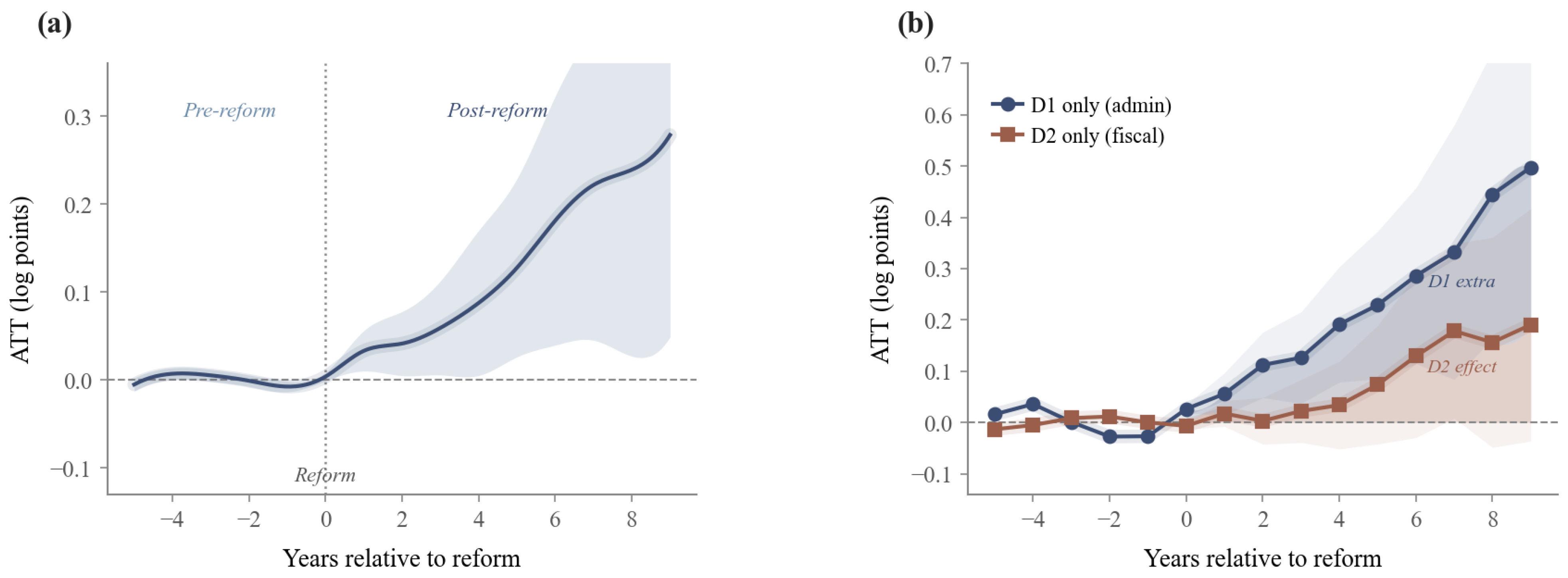
Figure 1 plots the dynamic ATT profile and the reform-type dynamic contrast.
Table 5 reports the relative-period estimates underlying the dynamic ATT profile. The counterfactual interpretation of the ATT depends on the quality of the pre-treatment fit. In the five years preceding reform ( h = 5 to h = 1 ), all point estimates are economically negligible, with the largest magnitude being 0.8 % at h = 1 , less than one-twentieth of the main post-reform ATT. Two periods show marginal statistical significance: h = 4 (ATT = 0.007, p = 0.039 ) and h = 1 (ATT = −0.008, p = 0.013 ). We do not interpret these as evidence of meaningful pre-trends for three reasons. The magnitudes are small, below 1% in percentage terms. The two effects point in opposite directions, inconsistent with any systematic upward or downward pre-trend. The gsynth factor model ( r = 2 ) also absorbs unit-specific pre-treatment trajectories, so residual pre-treatment estimates may reflect estimation noise. The mean absolute pre-treatment ATT over h = 5 to 1 is approximately 0.005, compared with a period-weighted post-reform average of 0.160, consistent with good pre-period fit.
The shape of the dynamic ATT trajectory is informative, but it should be interpreted within the preferred factor specification. The reform year itself ( h = 0 ) generates a negligible and insignificant effect (0.4%), consistent with the administrative and institutional lag inherent in budget procedures, since counties need at least one full fiscal cycle to operationalize the reformed governance channel. Effects then increase from h = + 1 (3.4%) through h = + 9 (32.1%), with the steepening evident from h = + 4 onward. This pattern is consistent with the gradual institutionalization of direct province–county fiscal relationships, expanding project pipelines under new administrative authority, and accumulating intergovernmental transfer flows. It is less consistent with a purely one-time rerouting interpretation, but it does not by itself identify a single mechanism. Confidence intervals widen sharply after h = + 9 as the number of contributing counties falls below 700, so the credible window of inference runs from h = + 1 to h = + 9 .

3.3. Robustness

The credibility of the main ATT depends on how it behaves under alternative estimators, sample restrictions, and factor-number choices.
The MC estimator supports the positive direction of the effect (ATT = 0.078, p < 0.001 ), but its smaller magnitude makes clear that the 16.7% gsynth estimate should be interpreted as the preferred-specification estimate rather than as a model-invariant quantity. The gsynth–MC gap reflects differences in each estimator’s adjustment for unobserved heterogeneity under the specific data-generating process documented in Table 3.
Factor-number sensitivity is the main limitation of the average-effect estimate. Table 6 reports the factor-number sensitivity estimates. The cross-validation curve shows a V-shape: MSPE declines from r = 0 (0.028) to r = 2 (0.023) and then rises sharply to r = 3 (0.092), identifying r = 2 as the cross-validated optimum. However, fixing r = 1 produces ATT = 0.066 (SE = 0.035, p = 0.061 ), while fixing r = 3 produces ATT = 0.011 (SE = 0.051, p = 0.837 ). This instability should be interpreted substantively, not only as a tuning issue. The r = 1 model is likely too parsimonious to absorb heterogeneous county trajectories in a two-decade staggered rollout, leaving residual pre-treatment structure in the estimated gap. The r = 3 model may move in the opposite direction by absorbing part of the post-reform variation into the latent factor structure. The r = 2 estimate has the strongest in-sample support by MSPE and pre-treatment fit, but the sensitivity across factor choices prevents us from treating 0.154 as a model-invariant magnitude. The more defensible conclusion is that the preferred specification and Matrix Completion benchmark support a positive average expenditure effect, while the exact magnitude remains model-dependent.
To address province-specific price changes directly, we constructed a province-year CPI deflator from the official China Statistical Yearbook consumer price indices by region (preceding year = 100), normalized each province’s price path to 2000 = 1, and re-estimated the main gsynth model using log CPI-deflated per-capita fiscal expenditure. This robustness check keeps the same 2000–2019 window and selects two latent factors. The internal gsynth estimation matrix is the same as in the nominal main model: 1729 counties, 873 treated counties, and 856 never-treated controls. The estimated ATT remains positive and statistically significant (ATT = 0.137, SE = 0.050, 95% CI: [0.038, 0.236], p = 0.007 ), equivalent to a 14.7% increase. Because provincial CPI applies one price path to all counties within a province, this result should be read as a province-price-path adjustment rather than a county-level public-service cost deflator. It nevertheless indicates that the positive average estimate is not driven solely by province-level CPI differences (Supplementary Table S5).
Under alternative coverage thresholds of 30% and 70%, panel fixed-effects estimates remain consistent in sign, providing limited support for robustness to the sample restriction. The relative-time event-study diagnostics also support a cautious interpretation of the staggered design: in the five years before adoption, the mean absolute pre-treatment ATT is 0.005 in the pooled gsynth model, compared with a period-weighted post-reform average of 0.160. Two pre-period coefficients are statistically significant, but their magnitudes are below 1%, and they point in opposite directions. Overall, the average-effect evidence supports a positive preferred-specification estimate, while the exact magnitude remains sensitive to modeling choices. The next question is whether the two institutional dimensions of PMC reform, administrative power delegation and fiscal direct reporting, show different empirical patterns.
The original research design anticipated a second gsynth analysis of reform effects on county log GDP per capita. Preliminary assessment showed substantial selection in the available GDP subsample, with reform counties over-represented at a 57% treatment rate versus 33% among excluded counties, which would compromise counterfactual construction under the factor structure assumption. As a non-causal descriptive alternative, we estimated a county and year fixed-effects model for log GDP per capita in the selected GDP subsample. The reform coefficient is small and statistically insignificant ( β = 0.003 , SE = 0.013, p = 0.810 ). We therefore do not report GDP as a causal outcome and focus the counterfactual analysis on county fiscal expenditure.

3.4. Heterogeneous Treatment Effects

Administrative power delegation (D1) and fiscal direct reporting (D2) show different point estimates in separate gsynth models, with D1’s ATT (0.262) larger than D2’s (0.103). This contrast should be interpreted cautiously because D1 and D2 counties differ at baseline and because the two institutional components may be temporally or functionally interdependent. Table 7 presents the reform-type gsynth estimates, with each group evaluated against the full control pool ( N = 856 ). Group-specific dynamic estimates provide an additional pre-treatment diagnostic: the mean absolute pre-treatment ATT over h = 5 to h = 1 is 0.021 for D1-only counties and 0.008 for D2-only counties. These magnitudes are small relative to the post-treatment estimates, but several D1 pre-period coefficients are statistically significant, so we do not interpret the D1–D2 gap as a clean causal ranking. We do not add matching or reweighting as primary D1–D2 evidence because those checks would shift the estimand toward a narrower overlap population while leaving the temporal and functional interdependence between D1 and D2 unresolved. Because a direct covariance estimate for the two separately estimated ATT parameters is not available, we conduct a complementary equality test using county-level post-treatment CATEs extracted from the common main gsynth model. This common-model test compares D1-only and D2-only counties under the same fitted counterfactual structure, but it does not establish that D1 causally dominates D2 under all institutional conditions. Table 8 summarizes the group-specific pre-treatment fit diagnostics that motivate this cautious interpretation.
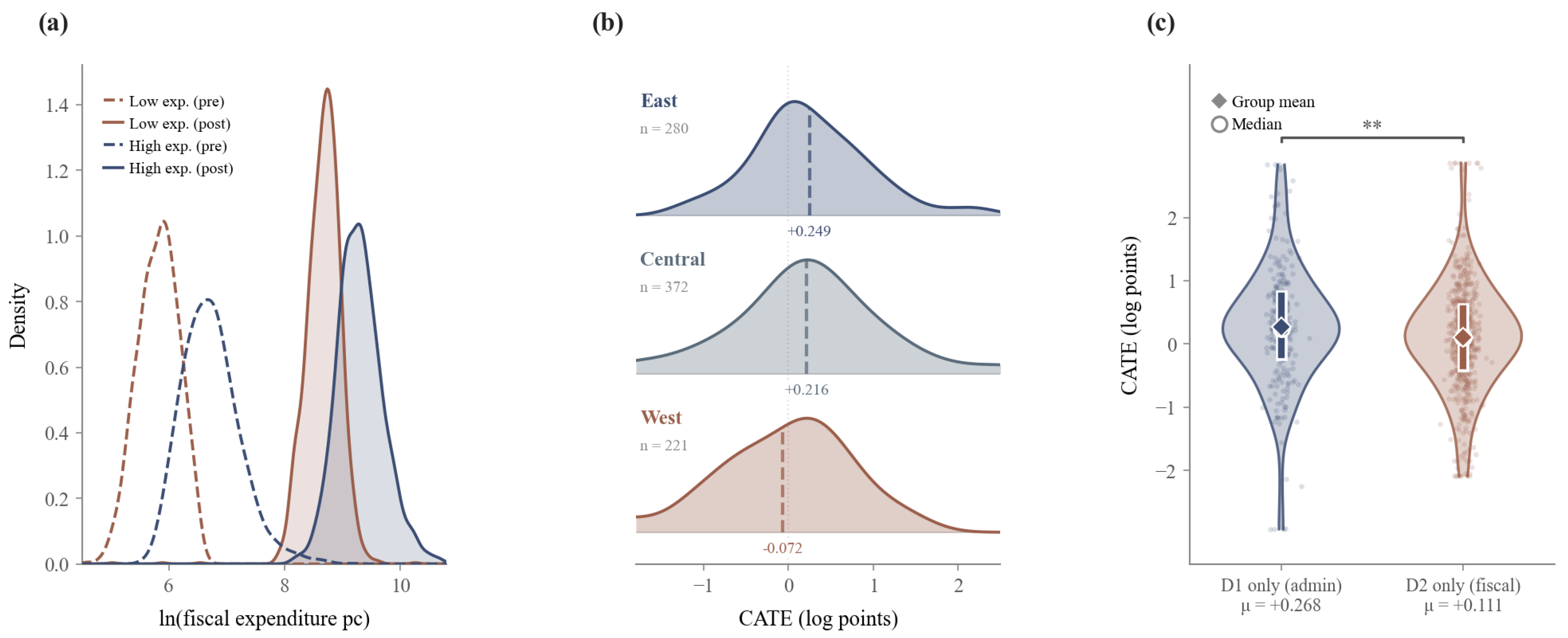
Administrative power delegation (D1) has the largest estimated ATT in Table 7, a 29.9% increase in per-capita fiscal expenditure (ATT = 0.262, p < 0.001 ). Using the same pre-reform baseline scale as above, this is roughly 183 yuan per capita at the mean baseline and 149 yuan at the median baseline. The common-model CATE equality test in Table 9 is consistent with the D1–D2 contrast: the D1-only mean CATE exceeds the D2-only mean CATE by 0.157 log points (bootstrap-error SE = 0.075, p = 0.037 ; permutation p = 0.026 ). A plausible interpretation is that D1 operates partly through decision authority. By reducing the prefecture’s role in land-use, investment, and enterprise registration approvals, county governments gain more room to act on local economic opportunities. The violin plots in Figure 2c suggest that D1’s larger mean estimate comes mainly from a thicker upper tail. This pattern supports the systems hypothesis that decision-right architecture can matter for fiscal expenditure output, while remaining short of a definitive causal ranking of D1 and D2.
Fiscal direct reporting (D2) produces a positive but smaller effect (ATT = 0.103, 10.9% increase), statistically significant at the 10% level ( p = 0.051 ). On the same baseline scale, this is roughly 66 yuan per capita at the mean baseline and 54 yuan at the median baseline. D2’s weaker effect may reflect the fact that rerouting fiscal accounting, while important for reducing prefecture interception of transfers, does not directly expand counties’ administrative decision space. Counties may receive modestly higher transfers but face similar approval bottlenecks in deploying those resources without accompanying administrative empowerment. The D2 estimate is also more heterogeneous, with the 95% CI spanning from effectively zero (−0.001) to 20.7%, suggesting that the effectiveness of D2 reform varies with local context.
The D1∩D2 row is retained only to document why no complementarity inference is possible. The group contains only N = 10 treated counties in the estimation sample, all from Henan Province, and the estimate is statistically uninformative given the extremely wide confidence interval (95% CI: [−0.240, 0.356]). We do not generalize from this small cell and do not use it to infer whether D1 and D2 are complementary. Future work in provinces with larger simultaneous dual-reform rollouts could estimate the complementarity parameter more credibly. The D1 versus D2 differential is consistent with the interpretation that administrative decision authority may be a more important constraint than fiscal-flow channels for many county governments. Whether this institutional heterogeneity also maps onto China’s geographic landscape, where the uneven spatial distribution of reform types corresponds to big structural differences in regional governance capacity, is the question the following section addresses.
The regional diagnostics are consistent with the broader interpretation that institutional context conditions reform absorption, but they do not support a simple region-ranking conclusion. Panel fixed-effects estimates stratified by Eastern, Central, and Western China provide a descriptive within-county comparison. Western counties ( N = 611 ) show a larger descriptive association in the FE estimates ( β = 0.107 , SE = 0.018, p < 0.001 ), Eastern counties ( N = 696 ) show a smaller statistically significant positive association ( β = 0.043 , SE = 0.016, p = 0.008 ), and Central counties ( N = 695 ) show a near-zero association ( β = 0.000 , SE = 0.012, p = 0.988 ). These estimates are conditional correlations rather than regional counterfactual effects. Table 10 reports the descriptive regional fixed-effects estimates.
To avoid relying only on region-specific FE benchmarks, Table 11 summarizes county-level CATEs extracted from the common main gsynth model. This diagnostic uses the same fitted counterfactual structure for all treated counties. The common-model CATEs show positive median effects in all three regions, but the regional ranking differs from the FE comparison: Eastern and Central regions have larger mean CATEs than the Western region, while the Western region has a positive median but a negative mean because of a heavier lower tail. We therefore interpret the regional evidence as showing geographically uneven absorption of PMC reform, not as establishing that any one region has a robustly larger causal effect across all specifications.
This logic extends from geographic regions to the within-region expenditure distribution, where counties at the bottom of the expenditure spectrum may face a structural disadvantage in leveraging the new institutional framework. The unconditional quantile analysis examines this distributional pattern.
The aggregate regional pattern masks a within-distribution pattern with important implications for system performance. In the broader UQR sample, PMC reform is associated with larger estimated gains among counties near the middle and top of the expenditure distribution, while lower-tail effects are weak or negative. The panel unconditional quantile regression estimates no significant effect at Q10 (0.6%, p = 0.252 ), a small negative effect at Q25 ( 2.1 % , p = 0.029 ), and positive coefficients at Q50–Q90 (19.7% to 25.0%, all p < 0.001 ). Because the UQR sample differs from the gsynth main sample, these estimates are interpreted as distributional evidence from a broader panel rather than as direct decompositions of the gsynth ATT. Table 12 and Figure 2a report the full panel UQR estimates.
The distributional results suggest a marked difference in reform incidence within the UQR sample. At Q10, the coefficient is near zero and statistically insignificant (0.006, p = 0.252 ). At Q25, reform is associated with a small reduction in per-capita fiscal expenditure (ATT = 0.021 , p = 0.029 ). From the median upward, reform is associated with positive effects: 25.0% at Q50, 24.5% at Q75, and 19.7% at Q90.
The distributional pattern therefore does not support a strong bottom-decile loss claim; instead, it supports the more cautious conclusion that lower-tail counties do not share the large gains observed above the median. Several mechanisms may account for this pattern. Provinces may couple PMC reform implementation with minimum public service standards, which can force low-capacity counties to reallocate budgets across categories. Fiscal direct reporting also requires counties to negotiate directly with provincial finance bureaus, a relationship that may disadvantage low-expenditure and typically rural counties with weaker administrative capacity. Finally, D2-only reform is more common among lower-expenditure counties, while D1 is more common among middle-range counties, contributing mechanically to weaker lower-tail estimates. These interpretations remain mechanisms to be investigated rather than fully identified pathways.

3.5. Mechanism Analysis

The positive aggregate effect and its spatial and distributional heterogeneity motivate an exploratory mechanism analysis of the fiscal autonomy channel. The estimates point to a counterintuitive denominator pattern in which reform is associated with higher total expenditure and a lower measured fiscal autonomy ratio, complicating conventional welfare interpretations of decentralization. These estimates represent descriptive conditional correlations rather than causal effects; county and year fixed effects partial out time-invariant confounders and common shocks but cannot fully address time-varying selection. Table 13 presents the full results.
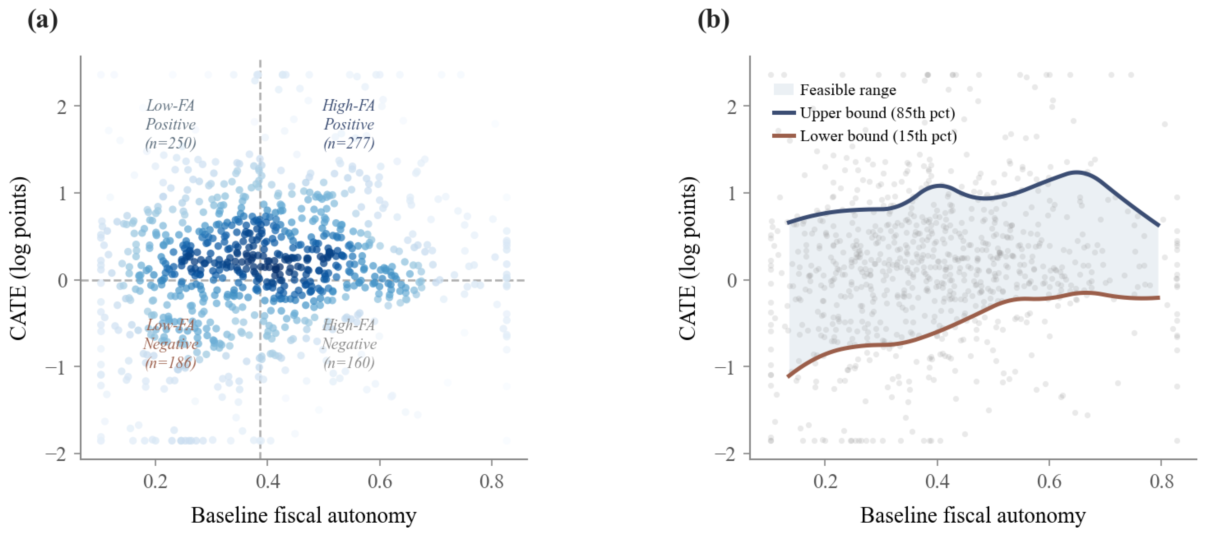
The relationship between reform and fiscal autonomy is documented in Table 13, Column 1 is consistent with a denominator effect that is counterintuitive but mechanically plausible. Reform is associated with a reduction in fiscal autonomy of 3.2 percentage points ( p < 0.001 ). This pattern could arise if PMC reform increases counties’ total expenditure faster than own-source revenue, mechanically reducing the ratio of own revenue to total expenditure. This interpretation is related to the fiscal federalism literature on the flypaper effect, in which intergovernmental transfers “stick” to local fiscal expenditure instead of being fully offset by reductions in local revenue effort [30]. It also differs from a pure substitution effect, under which added transfers would mainly replace own-source revenue without expanding total spending. In the PMC setting, a flypaper-style mechanism is plausible because D2 shortens the fiscal reporting path and can make provincial transfers more directly visible in county budgets. D1 can also increase counties’ ability to convert fiscal access into projects and services. The evidence in Table 13 remains descriptive, however; it supports consistency with a transfer-driven expenditure channel rather than identifying that channel causally.
Figure 3 visualizes the fiscal-autonomy diagnostics underlying this mechanism discussion.
China’s 2016 VAT reform is relevant because it replaced the business tax with a value-added tax and changed the distribution of tax bases between central and local governments, potentially altering local own-source revenue and transfer dependence. To check whether the denominator pattern is driven by this national fiscal shock, we split the mechanism sample at 2016. The Reform → FA association is statistically significant in the pre-VAT period 2000–2015 ( β = 0.041 , SE = 0.005, p < 0.001 ) and insignificant in the post-VAT period 2016–2019 ( β = 0.036 , SE = 0.048, p = 0.453 ). The post-period null partly reflects the shorter four-year window and reduced reform variation post-2015; the pre-VAT result suggests that the denominator pattern is not solely a post-2016 artifact.
The second column of Table 13 is consistent with a double-negative channel. Reform is associated with lower fiscal autonomy ( β 1 = 0.032 ), and fiscal autonomy is negatively associated with expenditure ( β 2 = 0.196 ). Counties with lower fiscal autonomy are more transfer-dependent and exhibit higher per-capita expenditure. One plausible explanation is that provincial transfers flow disproportionately to fiscally weaker counties to fund mandated services. The indirect association through the FA channel is positive but modest. The direct association between reform and expenditure conditional on FA is 0.037, and the combined panel-FE total is 0.043, substantially below the gsynth ATT of 0.154. This gap does not imply that the panel FE and gsynth estimates are inconsistent; they estimate different objects under different assumptions. Panel FE estimates the within-unit correlation between reform status and expenditure conditional on county and year fixed effects. By contrast, gsynth constructs the counterfactual of what expenditure would have been absent reform, accounting for time-varying unobservables that panel FE cannot absorb. The FA channel examined here represents one possible transmission pathway, not the complete explanation for the 16.7% preferred-specification expenditure increase. Other channels, including administrative empowerment effects on local investment and revenue mobilization, may contribute to the total gsynth ATT but lie outside the scope of the current mechanism analysis.
The third column tests the prefecture-level anchoring hypothesis with the variable city_control, defined as the inverse of the pre-reform variance in fiscal autonomy among non-reform counties within the same prefecture, where a higher value indicates a more fiscally homogeneous prefectural environment. The interaction between reform and this variable is negative and statistically insignificant ( β = 0.000029 ; SE = 0.000020; p = 0.142 ). The negative sign is directionally consistent with the hypothesis that reform is more effective in prefectures where surrounding counties exhibit low fiscal variance, but the effect is economically tiny and statistically imprecise, reflecting the extreme right-skewness of city_control and limited within-prefecture variation in reform status. We retain this as an exploratory test while acknowledging that the current measurement strategy lacks sufficient precision for credible inference. These mechanism regressions provide exploratory evidence on one possible aggregate pathway, but they necessarily average over pronounced individual heterogeneity that the gsynth model makes visible through its full matrix of county-level treatment effects.

3.6. Spatial Diagnostics of Estimated Treatment Effects

The estimated treatment effects are consistent with spatial clustering, suggesting that weaker and stronger estimated gains may be geographically patterned rather than purely idiosyncratic. The county-level Conditional Average Treatment Effects (CATE) extracted from the main gsynth model exhibit substantial heterogeneity across the 873 treated counties. Table 14 reports distributional statistics by reform type.
Three features of the CATE distribution suggest pronounced individual heterogeneity behind the aggregate ATT of 0.154. The unweighted post-treatment county mean (0.162) is close to the period-weighted ATT (0.154), suggesting that the average result is not driven solely by the weighting of early adopters. At the same time, the standard deviation (0.955) is large relative to the mean, indicating that county-level estimated effects are widely dispersed: the 10th percentile is −0.873 log points, while the 90th percentile is +1.121 log points. These tail estimates are generated quantities from the fitted gsynth model, so they should be interpreted as heterogeneity diagnostics rather than as precise county-level causal effects. The common model assigns positive estimated effects to all 10 D1∩D2 counties, but this Henan-only sample is too small for inference. The D1∩D2 CATE mean (0.527) also differs substantially from its separate four-group ATT in Table 7 (0.058) because the two statistics originate from different model specifications. The CATEs in Table 14 are extracted from the main combined-treatment model, which pools all 873 treated counties with r = 2 ; the ATT in Table 7 is estimated from a separate model with only 10 treated D1∩D2 units ( r = 3 ), where the counterfactual is less stable. We therefore do not draw inferential conclusions from either statistic for the D1∩D2 group.
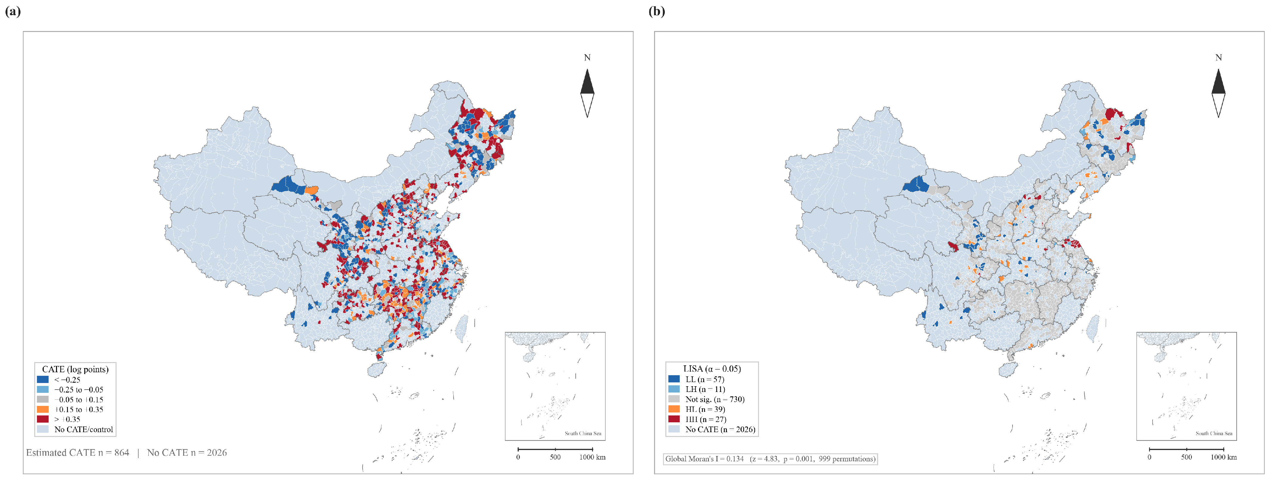
Exploratory spatial analysis of 864 estimated county-level post-treatment CATEs matched to the official standard-map service vector boundary base (map approval number: GS(2024)0650) is consistent with statistically significant geographic clustering (Global Moran’s I = 0.134 , z = 4.83 , p = 0.001 ). Because CATEs are model-estimated quantities, these spatial statistics should be read as diagnostics of the geography of estimated effects rather than as observed spatial outcomes. The nine treated counties excluded from the spatial analysis reflect county-code or boundary-version mismatches in the official vector base and account for only 1.0% of treated counties. LISA identifies 27 High-High clusters, 57 Low-Low clusters, 39 High-Low spatial outliers, 11 Low-High spatial outliers, and 730 counties not significant at the 5% level. The presence of both Low-Low and High-Low locations suggests that weak or contrastive estimated effects are spatially structured, but the analysis remains exploratory.
Figure 4a indicates that high and low estimated CATEs are interspersed across the reforming county belt, with visible concentrations in Central, Southwestern, and Northeastern counties. Negative estimated CATEs appear in parts of Central China and the Northeast, indicating that positive regional medians in the common-model diagnostics can still mask higher and lower estimated effects within the same region. The LISA map in Panel (b) reports that both HH and LL clusters satisfy the 5% permutation threshold; this supports an exploratory interpretation that estimated treatment effects are spatially patterned.
The spatial evidence complements the heterogeneity analysis, while remaining exploratory. The reform-type estimates suggest that administrative power delegation may be more consequential than fiscal direct reporting; the regional diagnostics suggest that this logic varies geographically; the UQR results indicate that lower-expenditure counties benefit much less than counties above the median; and the LISA clusters suggest that weak estimated effects are spatially concentrated. A reform with a positive preferred-specification average effect may therefore still produce uneven estimated gains across the county system if low-gain counties share similar institutional and regional environments.


4. Discussion

The main contribution of this paper is to translate PMC reform into a systems problem: how a multilevel governance system changes when intermediary nodes, decision rights, and fiscal-flow paths are reconfigured. In this view, county fiscal expenditure is not a standalone fiscal outcome. It is a system output produced by coupled relations among provincial resource allocation, prefectural mediation, county decision authority, and local implementation capacity. The preferred gsynth estimate is positive, but its magnitude is model-dependent. The more robust theoretical point is therefore not the exact percentage gain. It is that changing the architecture of authority and flow paths can alter local fiscal-output trajectories in a large hierarchical system.
The decomposition of PMC into D1 and D2 is the paper’s second systems contribution. A single reform dummy hides the distinction between changing what counties are allowed to decide and changing how fiscal resources are reported and settled. By separating these coupled subsystems, the analysis indicates that the same formal decentralization label can correspond to different system interventions with different estimated outputs. The quantile and spatial diagnostics extend this logic by indicating that architecture change is not absorbed uniformly across local subsystems. Lower-expenditure counties and spatially clustered low-gain counties appear less able to convert formal reform into large expenditure gains. This links systems thinking to counterfactual policy evaluation: the relevant question is not only whether a reform works on average, but which subsystem is reconfigured, through what coupling mechanism, and for which local parts of the larger governance system.
The D1–D2 contrast is central for theorizing about and evaluating PMC reform as a system redesign. Existing studies treat the reform as a unified intervention, effectively estimating a weighted average of two institutionally distinct changes. The four-group design and the common-model CATE equality test provide evidence that administrative power delegation has a larger estimated fiscal-expenditure effect than fiscal direct reporting, a pattern that prior unified indicators could not isolate because they did not separate the two dimensions. This is consistent with classic fiscal federalism arguments [31,32]: expenditure devolution unaccompanied by administrative devolution may fail to improve local service delivery because local governments lack the decision authority to act on new resources. In the Chinese context, D2-only counties may gain formal fiscal independence from the prefecture while remaining administratively subordinate. The implication is that changing fiscal-flow paths without changing decision rights may leave a core system constraint unresolved.
The distributional finding further suggests that the reform is not absorbed uniformly through the county system. Prud’homme warned that fiscal decentralization tends to produce winner-takes-more outcomes in developing country settings [33], and Rodden documented fiscal federalism dilemmas in which weaker subnational governments fail to benefit from devolution [34]. Our results suggest that the most constrained counties appear to gain far less than counties in the middle and upper parts of the distribution, with a small negative estimate at Q25 in the broader UQR sample. The Low-Low and High-Low estimated-CATE locations are geographically concentrated, consistent with affected counties sharing institutional environments that may suppress reform effectiveness regardless of formal adoption, including entrenched prefectural political economies, high legacy debt burdens, and narrowly scoped D1 delegation. This geographic structuring is consistent with the view that the same institutional rule can generate different local outcomes depending on the surrounding system environment.
The fiscal autonomy paradox connects to a broader measurement debate in the fiscal federalism literature [17,35]. Standard fiscal autonomy indicators conflate revenue capacity with fiscal independence, making them poorly suited to evaluate reforms that expand county expenditure primarily through vertical transfer channels rather than own-source revenue growth [36,37,38]. Our mechanism analysis, which finds that reform is associated with lower own-revenue shares while total expenditure is higher through a double-negative association, suggests that Chinese county fiscal health assessments anchored to autonomy ratios may misread the spending-capacity implications of hierarchy reform [15,18]. This pattern is consistent with a structural feature rather than a simple measurement artifact, since the transfer-expansion channel appears to be one plausible pathway through which PMC reform operates, especially in transfer-dependent local settings, although regional rankings vary across diagnostics. For systems analysis, the broader lesson is that an indicator can move in an apparently unfavorable direction while the functional capacity of a subsystem improves through a different channel.

5. Conclusions

The average-effect evidence supports a positive association between PMC reform and county per-capita fiscal expenditure in both the preferred gsynth specification and the Matrix Completion benchmark, but the exact magnitude remains model-dependent. The preferred gsynth specification corresponds to a 16.7% increase, while Matrix Completion gives a smaller 8.1% benchmark and factor-number sensitivity requires caution in interpreting the exact magnitude. The reform-type estimates and the common-model CATE equality test suggest that administrative power delegation may be more consequential than fiscal direct reporting, but this contrast should be read as institutional heterogeneity rather than definitive causal dominance. The distributional evidence from the broader UQR sample suggests no significant effect at Q10, a small negative effect at Q25, and positive estimates above the median, while the fiscal autonomy results suggest that reform may expand spending through transfer-driven expenditure growth even as the measured autonomy ratio falls. Together, these results suggest that PMC reform is a complex, uneven, and institutionally varied intervention in China’s intergovernmental fiscal system. In this paper, reform effectiveness is therefore defined narrowly as a change in county-recorded fiscal expenditure; it should not be read as direct evidence of fiscal equalization, service quality, welfare improvement, or real purchasing-power gains.
Three implications follow. For fiscal decentralization theory, the D1–D2 contrast is consistent with the long-theorized claim that administrative authority can be a key constraint on local service delivery, as counties can be freed from prefectural transfer interception while remaining institutionally incapable of converting new resources into expanded services without accompanying governance empowerment. For systems analysis, the results illustrate why policy evaluation should decompose multicomponent governance reforms into decision rights, fiscal-flow paths, and local implementation environments rather than treating reform adoption as a single binary state. For Chinese fiscal governance, the autonomy paradox implies that autonomy-ratio-based assessments may mischaracterize the spending-capacity implications of hierarchy reform, while the exploratory Low-Low and High-Low estimated-CATE locations highlight counties that formally received PMC reform but may remain constrained by prefectural political economy, legacy debt, or narrowly scoped delegation.
Several limitations constrain inference. The gsynth estimates are sensitive to latent factor choice: r = 1 yields a negative point estimate and r = 3 yields near-zero effects, so the r = 2 specification should be treated as the best-supported but not a model-invariant estimate. The group-specific D1 and D2 diagnostics also show small pre-treatment differences, reinforcing that the D1–D2 contrast should be read as institutional heterogeneity rather than causal dominance. The D1∩D2 group’s sample of ten counties, all from Henan Province, precludes credible inference on complementarity between the two reform dimensions. The mechanism regressions use panel fixed effects rather than a causal design, so the fiscal autonomy coefficients are conditional correlations rather than causal parameters. The UQR estimates use a broader sample than the main gsynth model and should therefore be interpreted as distributional evidence rather than as a direct decomposition of the main ATT. The D1–D2 equality test is based on common-model county-level CATEs rather than the covariance of separately estimated group-specific ATTs. The LISA analysis treats estimated CATEs as generated quantities and is exploratory. The GDP subsample is non-randomly selected, preventing counterfactual inference on economic development outcomes. Finally, the main outcome is nominal county-recorded fiscal expenditure; year effects and factor structures absorb common shocks, but they do not fully remove province-specific price changes or local cost differences.
Two research directions follow directly from these limitations and conclusions. First, provinces with larger simultaneous D1∩D2 rollouts would help assess whether coordinated dual-dimension implementation generates effects that are super-additive, testing whether administrative and fiscal empowerment are architecturally complementary or merely co-occurring. Second, as county-level GDP data quality improves, extending the counterfactual framework to economic development, land-use, migration, and rural income outcomes would permit assessment of whether the fiscal expenditure gains documented here translate into broader changes in the regional socio-economic system. A third direction is to construct comparable county-level public-service cost deflators, which would allow future work to distinguish nominal recorded expenditure from real service-provision capacity more directly than province-level CPI adjustment permits.

Supplementary Materials

The following supporting information can be downloaded at: https://www.mdpi.com/article/10.3390/systems14070819/s1. Table S1: county-year treatment-coding appendix; Table S2: D1–D2 CATE group summary; Table S3: D1–D2 common-model CATE equality test; Table S4: year-by-year observation counts for key variables; Table S5: provincial-CPI-deflated gsynth robustness check; Table S6: regional treatment-status distribution by Eastern/Central/Western and analytical sample scope; Table S7: regional common-model gsynth CATE diagnostics; Table S8: economic magnitude interpretation.

Author Contributions

Conceptualization, J.L., Y.W., S.W. and Z.D.; methodology, J.L. and S.W.; software, J.L.; formal analysis, J.L.; data curation, J.L.; writing—original draft preparation, J.L.; writing—review and editing, Y.W., S.W. and Z.D.; visualization, J.L.; supervision, Y.W., S.W. and Z.D.; project administration, Y.W. and S.W. All authors have read and agreed to the published version of the manuscript.

Funding

This research received no external funding.

Institutional Review Board Statement

Not applicable.

Informed Consent Statement

Not applicable.

Data Availability Statement

The full fiscal panel is available from the corresponding authors upon reasonable request, subject to source-data restrictions. A county-year treatment-coding appendix containing reform group, treatment status, D1/D2 indicators, and reform year is provided as Supplementary Material, together with the D1–D2 CATE group summary and the common-model CATE equality test summary.

Conflicts of Interest

The authors declare no conflicts of interest.

Abbreviations

The following abbreviations are used in this manuscript:
ATTAverage Treatment Effect on the Treated
CATEConditional Average Treatment Effect
D1Administrative Power Delegation
D2Fiscal Direct Reporting
FEFixed Effects
IFEInteractive Fixed Effects
LISALocal Indicators of Spatial Association
MCMatrix Completion
MSPEMean Squared Prediction Error
PMCProvince-Managing-County
RIFRecentered Influence Function
TWFETwo-Way Fixed Effects
UQRUnconditional Quantile Regression

References

  1. Zheng, S.; Sun, W.; Wu, J.; Kahn, M.E. The birth of edge cities in China: Measuring the effects of industrial parks policy. J. Urban Econ. 2017, 100, 80–103. [Google Scholar] [CrossRef]
  2. Jia, J.; Guo, Q.; Zhang, J. Fiscal decentralization and local expenditure policy in China. China Econ. Rev. 2014, 28, 107–122. [Google Scholar] [CrossRef]
  3. Huang, B.; Dong, Y.; Miao, J.; Xu, C. Intergovernmental fiscal transfers and county-level education expenditure in China. ECNU Rev. Educ. 2018, 1, 116–142. [Google Scholar] [CrossRef]
  4. Li, P.; Lu, Y.; Wang, J. Does flattening government improve economic performance? Evidence from China. J. Dev. Econ. 2016, 123, 18–37. [Google Scholar] [CrossRef]
  5. Liu, S.; Jin, Y.; Zhao, H. Reform of fiscal hierarchy and corporate innovation: Evidence from the “Province-Managing-County” fiscal reform in China. Pac.-Basin Financ. J. 2023, 80, 102068. [Google Scholar] [CrossRef]
  6. Sui, H.; Geng, S.; Zhou, J.; Raza, A.; Aziz, N. Fiscal institutional reform and export product quality: A quasi-experimental research on counties managed directly by provinces. Econ. Model. 2023, 126, 106383. [Google Scholar] [CrossRef]
  7. Ma, H.; Qin, C.; Zou, J.; Zhang, W. Fiscal decentralization and food production: Evidence from province-managing-county reform in China. China Econ. Rev. 2025, 90, 102342. [Google Scholar] [CrossRef]
  8. Liu, Z.; Zhong, H.; Zhen, D. Fiscal decentralization and land urbanization: Evidence from China’s fiscal reform of “province-managing-county”. Policy Stud. 2025, 1–29. [Google Scholar] [CrossRef]
  9. Zheng, X.; Zha, J.; Huang, Z. Administrative decentralization and firm entry: Evidence from China’s county power expansion reform. Appl. Econ. 2026; advance online publication. [CrossRef]
  10. Shen, H.; Cao, Z.; Liu, J. Administrative decentralization, government-firm interaction and firm pollution emissions. J. Clean. Prod. 2025, 519, 145952. [Google Scholar] [CrossRef]
  11. Goodman-Bacon, A. Difference-in-differences with variation in treatment timing. J. Econom. 2021, 225, 254–277. [Google Scholar] [CrossRef]
  12. Callaway, B.; Sant’Anna, P.H.C. Difference-in-differences with multiple time periods. J. Econom. 2021, 225, 200–230. [Google Scholar] [CrossRef]
  13. Sun, L.; Abraham, S. Estimating dynamic treatment effects in event studies with heterogeneous treatment effects. J. Econom. 2021, 225, 175–199. [Google Scholar] [CrossRef]
  14. de Chaisemartin, C.; D’Haultfœuille, X. Two-way fixed effects and differences-in-differences with heterogeneous treatment effects: A survey. Econom. J. 2023, 26, C1–C30. [Google Scholar] [CrossRef]
  15. Jiang, S.; Xu, A.; Zhang, X. Can budget performance management reform improve local fiscal resilience? Empirical evidence based on a quasi-natural experiment. SAGE Open 2025, 15, 21582440251386283. [Google Scholar] [CrossRef]
  16. Liu, Y.; Wu, R.; Huang, J.; Li, J. Research on the optimization of the intergovernmental sharing mechanism of public services under the new pattern of “dual circulation”. Int. Rev. Econ. Financ. 2025, 103, 104554. [Google Scholar] [CrossRef]
  17. Agrawal, D.R.; Brueckner, J.K.; Brülhart, M. Fiscal federalism in the twenty-first century. Annu. Rev. Econ. 2024, 16, 429–454. [Google Scholar] [CrossRef]
  18. Wang, Y.; Guo, L. Vertical fiscal imbalances, environmental regulations and resource allocation in the Chinese context. Appl. Econ. 2025, 57, 7196–7214. [Google Scholar] [CrossRef]
  19. Wooldridge, J.M. Two-way fixed effects, the two-way Mundlak regression, and difference-in-differences estimators. Empir. Econ. 2025, 69, 2545–2587. [Google Scholar] [CrossRef]
  20. Athey, S.; Imbens, G.W. Design-based analysis in difference-in-differences settings with staggered adoption. J. Econom. 2022, 226, 62–79. [Google Scholar] [CrossRef]
  21. Xu, Y. Generalized synthetic control method: Causal inference with interactive fixed effects models. Polit. Anal. 2017, 25, 57–76. [Google Scholar] [CrossRef]
  22. Athey, S.; Bayati, M.; Doudchenko, N.; Imbens, G.; Khosravi, K. Matrix completion methods for causal panel data models. J. Am. Stat. Assoc. 2021, 116, 1716–1730. [Google Scholar] [CrossRef]
  23. Abadie, A.; Diamond, A.; Hainmueller, J. Synthetic control methods for comparative case studies: Estimating the effect of California’s tobacco control program. J. Am. Stat. Assoc. 2010, 105, 493–505. [Google Scholar] [CrossRef]
  24. Arkhangelsky, D.; Athey, S.; Hirshberg, D.A.; Imbens, G.W.; Wager, S. Synthetic difference-in-differences. Am. Econ. Rev. 2021, 111, 4088–4118. [Google Scholar] [CrossRef]
  25. Liu, L.; Wang, Y.; Xu, Y. A practical guide to counterfactual estimators for causal inference with time-series cross-sectional data. Am. J. Polit. Sci. 2024, 68, 160–176. [Google Scholar] [CrossRef]
  26. Lechner, M. Causal machine learning and its use for public policy. Swiss J. Econ. Stat. 2023, 159, 8. [Google Scholar] [CrossRef]
  27. Canay, I.A. A simple approach to quantile regression for panel data. Econom. J. 2011, 14, 368–386. [Google Scholar] [CrossRef]
  28. Firpo, S.; Fortin, N.M.; Lemieux, T. Unconditional quantile regressions. Econometrica 2009, 77, 953–973. [Google Scholar] [CrossRef]
  29. Silverman, B.W. Density Estimation for Statistics and Data Analysis; Chapman & Hall: London, UK, 1986. [Google Scholar]
  30. Hines, J.R.; Thaler, R.H. Anomalies: The flypaper effect. J. Econ. Perspect. 1995, 9, 217–226. [Google Scholar] [CrossRef]
  31. Oates, W.E. An essay on fiscal federalism. J. Econ. Lit. 1999, 37, 1120–1149. [Google Scholar] [CrossRef]
  32. Bardhan, P. Decentralization of governance and development. J. Econ. Perspect. 2002, 16, 185–205. [Google Scholar] [CrossRef]
  33. Prud’homme, R. The dangers of decentralization. World Bank Res. Obs. 1995, 10, 201–220. [Google Scholar] [CrossRef]
  34. Rodden, J. The dilemma of fiscal federalism: Grants and fiscal performance around the world. Am. J. Polit. Sci. 2002, 46, 670–687. [Google Scholar] [CrossRef]
  35. Cantoni, D.; Mohr, C.; Weigand, M. The rise of fiscal capacity: Administration and state consolidation in the Holy Roman Empire. Econometrica 2024, 92, 1439–1472. [Google Scholar] [CrossRef]
  36. Lam, W.R.; Badia, M.M. Fiscal policy and the government balance sheet in China. Int. Rev. Econ. Financ. 2026, 106, 104950. [Google Scholar] [CrossRef]
  37. Chen, X.; Zhang, L.; Cheng, X. Fiscal decentralization and the development of the digital economy: Evidence from China. J. Econ. Policy Reform 2024, 27, 276–292. [Google Scholar] [CrossRef]
  38. Liu, R.; Liu, Z.; Li, J. Research on the impact of fiscal vertical imbalance on the green total factor productivity of enterprises. Sustainability 2026, 18, 1265. [Google Scholar] [CrossRef]
Figure 1. Dynamic counterfactual evidence for PMC reform. (a) Smooth ATT trajectory ( h = 5 to + 9 ): the near-flat pre-reform period is consistent with the fitted counterfactual; ATT rises from + 3.4 % at h = + 1 to + 32.1 % at h = + 9 in the preferred specification. (b) D1-only vs. D2-only dynamic ATT with colored gap fill: the blue fill above D2 visualizes the D1–D2 point-estimate gap.
Systems 14 00819 g001
Figure 2. Heterogeneity decomposition of PMC reform treatment effects. (a) Pre- and post-reform kernel density of ln(fiscal expenditure p.c.) by expenditure tercile: the high-expenditure group (blue) shifts right post-reform while the low-expenditure group (rust) shows minimal movement, consistent with the panel UQR estimates reported below. (b) CATE ridge plot by geographic region (Eastern/Central/Western): the distributions differ across regions, but they do not support a simple region-ranking conclusion. (c) D1-only vs. D2-only CATE violin plots with Mann–Whitney test: D1 exhibits a heavier upper tail relative to D2, visualizing the distributional contrast tested in Table 9. The bracket annotation in Panel (c) reports a Mann–Whitney test; ** denotes p < 0.05 .
Systems 14 00819 g002
Figure 3. Mechanism diagnostics. (a) Scatter plot of county CATE (gsynth) vs. baseline fiscal autonomy (FA), with a LOWESS fit line and 4-quadrant density shading: the upper-right quadrant (high FA, high CATE) and lower-left quadrant (low FA, low/negative CATE) contain the bulk of the mass, consistent with the negative FA-expenditure association documented in Column 2 of Table 13, where lower fiscal autonomy is associated with higher transfer-driven expenditure. (b) Constraint-line analysis: the colored line marks the prefecture fiscal constraint threshold; counties to the left (more constrained) exhibit lower CATEs on average, while counties crossing the threshold show a discrete upward shift, consistent with the interpretation that reform may be more effective when the prefecture fiscal constraint is relaxed. Blue dots in Panel (a) denote individual counties, and darker blue indicates higher point density.
Systems 14 00819 g003
Figure 4. Exploratory spatial distribution of estimated PMC reform treatment effects. (a) CATE choropleth map: red shading indicates high positive estimated county-level post-treatment average effects; blue shading indicates negative estimated CATEs; grey denotes control counties, unmatched counties, or counties without post-treatment CATE estimates. (b) LISA cluster map of estimated CATE spatial autocorrelation: High-High (HH) clusters (red, n = 27 ); Low-Low (LL) clusters (dark blue, n = 57 ); High-Low (HL) and Low-High (LH) spatial outliers ( n = 39 and 11, respectively); grey = not significant at the 5% level (999 conditional permutations). The base boundary, South China Sea inset, and maritime boundary lines use official standard-map service vector boundaries (map approval number: GS(2024)0650); no maritime boundary line is manually drawn. Global Moran’s I = 0.134 ( z = 4.83 , p = 0.001 ).
Systems 14 00819 g004
Table 1. Treatment Coding Protocol for D1, D2, and Joint Reform Status.
Coding IssueRule Used in the Analysis
D1 start yearFirst year in which provincial documents identify a county as receiving delegated administrative authority.
D2 start yearFirst year in which provincial documents identify a county as entering direct province–county fiscal settlement or direct fiscal reporting.
Province-wide documentsAll eligible counties in the province are assigned the stated effective year.
Pilot-county documentsOnly listed counties are assigned treatment in the stated year.
Joint D1∩D2 statusA county is coded as joint reform only once both D1 and D2 are simultaneously in place.
Entry and exitTreatment is absorbing after implementation; no official exit cases were found.
Partial implementationCounty-year coding follows the document scope and is reported in the supplementary treatment-coding appendix.
Notes: The protocol is based on provincial reform documents. The full county-year coding is reported in Supplementary Table S1.
Table 2. Analytical-sample construction and use in the manuscript.
Sample StageCountiesTreated/ControlUse and Restriction
Raw county panel22191056/1163County-level panel across 31 provinces before analytical restrictions.
Outcome-coverage sample1934Counties with at least 50% non-missing fiscal expenditure observations in 2000–2019.
Main gsynth sample1729873/856Outcome-coverage sample plus treated counties with reform year in 2002–2015, ensuring at least two pre-reform periods.
Main reform-type groups873258/605/10Treated counties in the main gsynth sample: D1-only, D2-only, and D1∩D2.
Panel UQR sample1912Broader distributional sample; retains the ≥50% outcome-coverage rule but not gsynth-specific timing restrictions.
Regional FE sample2002Counties with non-missing variables for descriptive regional panel fixed-effects estimates.
Spatial CATE sample864Treated counties with CATE estimates matched to the official standard-map service vector base.
Notes: Treated/control in the raw panel refers to final reform status by 2019. The full reform classification is 332 D1-only counties, 713 D2-only counties, 11 D1∩D2 counties, and 1163 never-treated controls. The main gsynth sample is smaller because of outcome-coverage and treatment-timing restrictions. The yearly number of non-missing fiscal-expenditure observations ranges from 1720 to 2016 in 2000–2019; the year-by-year counts are reported in Supplementary Table S4.
Table 3. Pre-reform baseline characteristics by group (2000–2005 means; SD in parentheses).
ControlD1 OnlyD2 OnlyD1∩D2
N (counties)116333271311
ln(fiscal exp pc)6.504 (0.650)6.290 (0.497)6.234 (0.392)5.788 (0.301)
Fiscal autonomy0.487 (0.273)0.479 (0.185)0.406 (0.188)0.450 (0.146)
Primary industry %25.0 (15.8)26.1 (12.8)31.7 (11.9)29.9 (13.3)
Secondary industry %39.4 (15.6)41.7 (13.8)35.8 (12.6)42.9 (13.6)
ln(population)3.533 (0.818)3.957 (0.643)3.715 (0.692)4.679 (0.260)
Notes: Baseline averages computed over 2000–2005 for counties with non-missing data. Groups defined by whether counties received administrative power delegation (D1), fiscal direct reporting (D2), both, or neither, by 2019. Fiscal autonomy = own-source revenue/total expenditure.
Table 4. Main estimates: effect of PMC reform on ln(fiscal expenditure per capita).
(1) Gsynth(2) MC
ATT0.154 ***0.078 ***
SE(0.050)(0.011)
95% CI[0.056, 0.253][0.056, 0.100]
p-value0.002<0.001
% increase ( e ATT 1 )+16.7%+8.1%
Latent factors r2 (CV-selected)— (MC)
Treated counties ( N t r )873873
Control counties ( N c o )856856
County-year obs.36,14336,143
Years2000–20192000–2019
Notes: Column (1): gsynth. r = 2 selected by cross-validation (MSPE minimization). 1000 parametric bootstrap iterations. Column (2): Matrix Completion, cross-validated regularization, 200 bootstrap iterations. Two-way fixed effects imposed in both specifications. Control variables: ln(population). Significance: *** p < 0.01 .
Table 5. Dynamic ATT estimates: period-by-period gsynth estimates ( h = 5 to h = + 9 ).
Period hATTSE95% CI% ChangeNSig.
5 −0.0050.004[−0.013, 0.002]−0.5%808
4 +0.0070.003[+0.000, +0.014]+0.7%872*
3 +0.0050.003[−0.002, +0.012]+0.5%873
2 −0.0010.003[−0.007, +0.006]−0.1%873
1 −0.0080.003[−0.014, −0.002]−0.8%873*
0+0.0040.003[−0.001, +0.009]+0.4%873
+1+0.0330.012[+0.010, +0.056]+3.4%873***
+2+0.0410.019[+0.005, +0.078]+4.2%861**
+3+0.0590.027[+0.006, +0.113]+6.1%855**
+4+0.0880.042[+0.005, +0.170]+9.2%826**
+5+0.1280.052[+0.026, +0.229]+13.6%795**
+6+0.1810.072[+0.040, +0.323]+19.9%778**
+7+0.2220.090[+0.045, +0.398]+24.8%742**
+8+0.2390.108[+0.027, +0.451]+27.0%706**
+9+0.2790.117[+0.049, +0.508]+32.1%696**
Notes: Estimates from gsynth with r = 2 . % change = e ATT 1 . N = number of treated counties contributing observations at each relative period. Estimates at h 10 are omitted due to rapidly declining sample size ( N 610 ). * p < 0.10 , ** p < 0.05 , *** p < 0.01 .
Table 6. Factor-number sensitivity: gsynth ATT estimates under r = 0 , 1 , 2 , 3 .
rCV-MSPEATTSEp-ValueInterpretation
00.028No factor adjustment (TWFE)
10.025−0.0660.0350.061Under-fitted; absorbs residual pre-trend downward
20.023+0.1540.0500.002CV-selected optimum
30.092+0.0110.0510.837Over-fitted; may absorb post-reform variation
Notes: MSPE = cross-validated mean squared prediction error. The V-shape identifies r = 2 as the cross-validated optimum, while the ATT sensitivity across factor choices is an important limitation.
Table 7. Reform-type gsynth estimates and D1∩D2 small-cell diagnostic.
Reform TypeNATTSE95% CI% Changep-Value
D1 only (admin. power delegation)2580.2620.062[0.141, 0.384]+29.9%<0.001 ***
D2 only (fiscal direct reporting)6050.1030.053[−0.001, 0.207]+10.9%0.051 *
D1∩D2 (both reforms)100.0580.152[−0.240, 0.356]+6.0%0.705
Notes: Each group estimated separately against the common control pool ( N = 856 counties). N = number of treated counties. Standard errors from 500 (D1, D2) and 200 (D1∩D2) parametric bootstrap iterations. The D1∩D2 result is uninformative due to the very small treated-group sample. Significance: * p < 0.10 , *** p < 0.01 .
Table 8. Group-specific pre-treatment fit diagnostics for reform-type gsynth models.
Reform TypeNMean Abs. Pre-ATTInterpretation
D1 only2580.021Small relative to the post-treatment ATT, but several D1 pre-period coefficients are statistically significant; the D1–D2 contrast should therefore be interpreted cautiously.
D2 only6050.008Pre-treatment fit is closer to zero; the D2 point estimate remains smaller and less precise.
D1∩D210Small Henan-only cell; reported as a small-cell diagnostic rather than as evidence on complementarity.
Notes: mean absolute pre-treatment ATT is calculated over relative periods h = 5 to h = 1 in the group-specific dynamic estimates. The table is a diagnostic and is not used as a balance correction.
Table 9. Common-model CATE equality test: D1-only versus D2-only counties.
StatisticValue
Mean CATE, D1-only counties0.268
Mean CATE, D2-only counties0.111
D1–D2 difference0.157
Bootstrap-error SE0.075
z statistic2.086
p-value, bootstrap-error normal test0.037
p-value, county-label permutation test0.026
Notes: CATEs are county-level mean post-treatment effects extracted from the common main gsynth model. The bootstrap-error SE uses the 1000 parametric bootstrap draws stored in the main gsynth object. The permutation test randomly reassigns D1-only/D2-only labels across treated counties 10,000 times while preserving group sizes.
Table 10. Panel fixed-effects estimates by region.
RegionN Counties β (FE)SEp-Value
Western6110.1070.018<0.001
Eastern6960.0430.0160.008
Central6950.0000.0120.988
Notes: Panel fixed-effects estimates (county + year FE, SE clustered by county). Region defined by standard National Bureau of Statistics classification. These are descriptive conditional correlations. The main counterfactual evidence comes from the pooled gsynth model and the common-model CATE diagnostics below.
Table 11. Regional diagnostics based on common-model gsynth CATEs.
RegionTreated CountiesMean CATEMedian CATEPositive ShareMedian % Change
Eastern2800.2560.16661.4%18.1%
Central3720.2230.21063.7%23.4%
Western221−0.0590.05753.4%5.8%
Notes: CATEs are county-level mean post-treatment effects extracted from the common main gsynth model. Positive share is the share of treated counties with positive estimated CATE. The table is a regional diagnostic under a common counterfactual model, not a separate region-specific gsynth estimation.
Table 12. Panel UQR: distributional effect of PMC reform.
QuantileATTSE95% CI% ChangeSig.
Q10+0.0060.006[−0.005, +0.017]+0.6%
Q25−0.0210.010[−0.040, −0.002] 2.1 % **
Q50+0.2230.020[+0.184, +0.262]+25.0%***
Q75+0.2190.018[+0.183, +0.255]+24.5%***
Q90+0.1800.016[+0.150, +0.211]+19.7%***
Notes: Two-step Canay estimator. Step 1: county fixed effects removed via feols (within demeaning). Step 2: RIF regression on demeaned outcome. SE clustered by county. Year FE included. N = 1912 counties. The UQR sample retains the ≥50% outcome-coverage rule but does not impose gsynth-specific treatment-timing restrictions. ** p < 0.05 , *** p < 0.01 .
Table 13. Mechanism analysis: panel fixed-effects (county + year FE).
(1) Fiscal Autonomy(2) ln Expenditure(3) ln Expenditure
Reform (D)−0.032 ***+0.037 ***+0.058 ***
(0.005)(0.009)(0.012)
Fiscal autonomy (FA)−0.196 ***−0.187 ***
(0.032)(0.032)
D × city_control−0.000029
(0.000020)
County + Year FE
N (counties)∼2002∼2002∼1400
R 2 (within)0.1140.8910.891
Notes: Base-year industry ratios and ln(population) included as controls. SE clustered by county. city_control = inverse of the pre-reform within-prefecture variance in fiscal autonomy among non-reform counties (higher values indicate a more fiscally homogeneous prefectural environment); winsorized at the 99th percentile to limit the influence of extreme outliers. ✓ indicates included fixed effects; *** p < 0.01 .
Table 14. CATE distribution by reform type.
Reform TypeNMeanSDP10P50P90% Positive
D1 only258+0.2680.952−0.768+0.250+1.33666.7%
D2 only605+0.1110.960−0.902+0.110+1.05857.0%
D1∩D210+0.5270.218+0.264+0.504+0.746100.0%
All treated873+0.1620.955−0.873+0.154+1.12160.4%
Notes: CATE = county-level Conditional Average Treatment Effect over post-reform periods, extracted from the gsynth effect matrix (column means for treated counties). SD = standard deviation. P10/P50/P90 = 10th/50th/90th percentiles.
Disclaimer/Publisher’s Note: The statements, opinions and data contained in all publications are solely those of the individual author(s) and contributor(s) and not of MDPI and/or the editor(s). MDPI and/or the editor(s) disclaim responsibility for any injury to people or property resulting from any ideas, methods, instructions or products referred to in the content.