3.2. Average Treatment Effect: Magnitude and Dynamics
The preferred generalized synthetic control specification selects two latent factors through cross-validated MSPE minimization (: 0.028, : 0.025, : 0.023, : 0.092). The resulting ATT is 0.154 (SE = 0.050; 95% CI: [0.056, 0.253]; ). Interpreted within this specification, the estimate corresponds to an average post-reform expenditure increase of approximately 16.7%. This magnitude should not be read as a model-invariant effect size. The sensitivity analysis below indicates that the estimate changes substantially with the number of latent factors, and the Matrix Completion benchmark is smaller. The estimate is based on 873 treated counties benchmarked against 856 control counties over 2000–2019. The 873 treated counties represent the estimation sample after applying a 50% or greater temporal coverage filter and restricting reform timing to 2002–2015 to ensure adequate pre-treatment periods. The 332/713/11 breakdown in the broader classification reflects the full sample prior to these restrictions. One D1∩D2 county is further excluded by the coverage filter, reducing the D1∩D2 estimation group from 11 to 10 counties.
Table 4 summarizes the preferred gsynth and Matrix Completion estimates. The Matrix Completion estimator, which requires no parametric factor structure and imposes only low-rank Matrix Completion, produces a smaller statistically significant ATT of 0.078 (SE = 0.011; 95% CI: [0.056, 0.100];
), equivalent to an 8.1% increase. The gsynth–MC gap shows that the estimated magnitude depends on how unobserved heterogeneity is modeled. We therefore interpret the evidence as supporting a positive average effect in the preferred specification and robustness benchmark, while treating the exact size of the average effect as model-dependent.
For scale interpretation, the treated counties in the pre-reform baseline window 2000–2005 had an average county fiscal expenditure of approximately 610 yuan per capita, with a median of approximately 497 yuan. If the preferred gsynth estimate is applied to this baseline scale, a 16.7% increase corresponds to roughly 102 yuan per capita at the mean baseline, or 83 yuan at the median baseline. The Matrix Completion benchmark of 8.1% corresponds to roughly 50 yuan per capita at the mean baseline. These translations are intended only to convey economic magnitude; they are not interpreted as real-yuan welfare gains or changes in service quality.
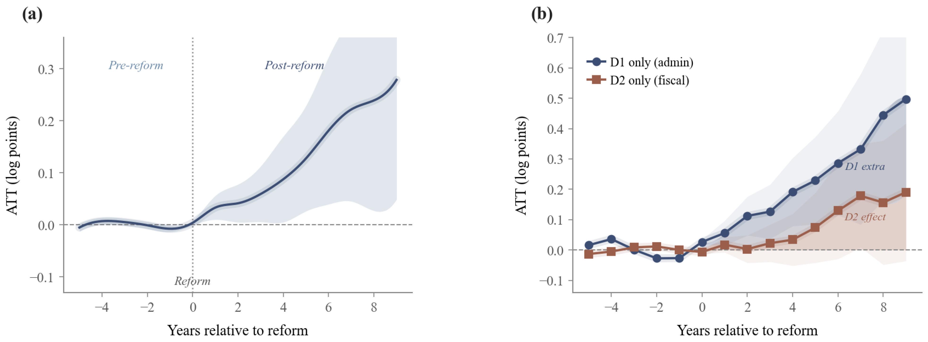
Figure 1 plots the dynamic ATT profile and the reform-type dynamic contrast.
Table 5 reports the relative-period estimates underlying the dynamic ATT profile. The counterfactual interpretation of the ATT depends on the quality of the pre-treatment fit. In the five years preceding reform (
to
), all point estimates are economically negligible, with the largest magnitude being
at
, less than one-twentieth of the main post-reform ATT. Two periods show marginal statistical significance:
(ATT = 0.007,
) and
(ATT = −0.008,
). We do not interpret these as evidence of meaningful pre-trends for three reasons. The magnitudes are small, below 1% in percentage terms. The two effects point in opposite directions, inconsistent with any systematic upward or downward pre-trend. The gsynth factor model (
) also absorbs unit-specific pre-treatment trajectories, so residual pre-treatment estimates may reflect estimation noise. The mean absolute pre-treatment ATT over
to
is approximately 0.005, compared with a period-weighted post-reform average of 0.160, consistent with good pre-period fit.
The shape of the dynamic ATT trajectory is informative, but it should be interpreted within the preferred factor specification. The reform year itself () generates a negligible and insignificant effect (0.4%), consistent with the administrative and institutional lag inherent in budget procedures, since counties need at least one full fiscal cycle to operationalize the reformed governance channel. Effects then increase from (3.4%) through (32.1%), with the steepening evident from onward. This pattern is consistent with the gradual institutionalization of direct province–county fiscal relationships, expanding project pipelines under new administrative authority, and accumulating intergovernmental transfer flows. It is less consistent with a purely one-time rerouting interpretation, but it does not by itself identify a single mechanism. Confidence intervals widen sharply after as the number of contributing counties falls below 700, so the credible window of inference runs from to .
3.3. Robustness
The credibility of the main ATT depends on how it behaves under alternative estimators, sample restrictions, and factor-number choices.
The MC estimator supports the positive direction of the effect (ATT = 0.078,
), but its smaller magnitude makes clear that the 16.7% gsynth estimate should be interpreted as the preferred-specification estimate rather than as a model-invariant quantity. The gsynth–MC gap reflects differences in each estimator’s adjustment for unobserved heterogeneity under the specific data-generating process documented in
Table 3.
Factor-number sensitivity is the main limitation of the average-effect estimate.
Table 6 reports the factor-number sensitivity estimates. The cross-validation curve shows a V-shape: MSPE declines from
(0.028) to
(0.023) and then rises sharply to
(0.092), identifying
as the cross-validated optimum. However, fixing
produces ATT
(SE = 0.035,
), while fixing
produces ATT
(SE = 0.051,
). This instability should be interpreted substantively, not only as a tuning issue. The
model is likely too parsimonious to absorb heterogeneous county trajectories in a two-decade staggered rollout, leaving residual pre-treatment structure in the estimated gap. The
model may move in the opposite direction by absorbing part of the post-reform variation into the latent factor structure. The
estimate has the strongest in-sample support by MSPE and pre-treatment fit, but the sensitivity across factor choices prevents us from treating 0.154 as a model-invariant magnitude. The more defensible conclusion is that the preferred specification and Matrix Completion benchmark support a positive average expenditure effect, while the exact magnitude remains model-dependent.
To address province-specific price changes directly, we constructed a province-year CPI deflator from the official China Statistical Yearbook consumer price indices by region (preceding year = 100), normalized each province’s price path to 2000 = 1, and re-estimated the main gsynth model using log CPI-deflated per-capita fiscal expenditure. This robustness check keeps the same 2000–2019 window and selects two latent factors. The internal gsynth estimation matrix is the same as in the nominal main model: 1729 counties, 873 treated counties, and 856 never-treated controls. The estimated ATT remains positive and statistically significant (ATT = 0.137, SE = 0.050, 95% CI: [0.038, 0.236],
), equivalent to a 14.7% increase. Because provincial CPI applies one price path to all counties within a province, this result should be read as a province-price-path adjustment rather than a county-level public-service cost deflator. It nevertheless indicates that the positive average estimate is not driven solely by province-level CPI differences (
Supplementary Table S5).
Under alternative coverage thresholds of 30% and 70%, panel fixed-effects estimates remain consistent in sign, providing limited support for robustness to the sample restriction. The relative-time event-study diagnostics also support a cautious interpretation of the staggered design: in the five years before adoption, the mean absolute pre-treatment ATT is 0.005 in the pooled gsynth model, compared with a period-weighted post-reform average of 0.160. Two pre-period coefficients are statistically significant, but their magnitudes are below 1%, and they point in opposite directions. Overall, the average-effect evidence supports a positive preferred-specification estimate, while the exact magnitude remains sensitive to modeling choices. The next question is whether the two institutional dimensions of PMC reform, administrative power delegation and fiscal direct reporting, show different empirical patterns.
The original research design anticipated a second gsynth analysis of reform effects on county log GDP per capita. Preliminary assessment showed substantial selection in the available GDP subsample, with reform counties over-represented at a 57% treatment rate versus 33% among excluded counties, which would compromise counterfactual construction under the factor structure assumption. As a non-causal descriptive alternative, we estimated a county and year fixed-effects model for log GDP per capita in the selected GDP subsample. The reform coefficient is small and statistically insignificant (, SE = 0.013, ). We therefore do not report GDP as a causal outcome and focus the counterfactual analysis on county fiscal expenditure.
3.4. Heterogeneous Treatment Effects
Administrative power delegation (D1) and fiscal direct reporting (D2) show different point estimates in separate gsynth models, with D1’s ATT (0.262) larger than D2’s (0.103). This contrast should be interpreted cautiously because D1 and D2 counties differ at baseline and because the two institutional components may be temporally or functionally interdependent.
Table 7 presents the reform-type gsynth estimates, with each group evaluated against the full control pool (
). Group-specific dynamic estimates provide an additional pre-treatment diagnostic: the mean absolute pre-treatment ATT over
to
is 0.021 for D1-only counties and 0.008 for D2-only counties. These magnitudes are small relative to the post-treatment estimates, but several D1 pre-period coefficients are statistically significant, so we do not interpret the D1–D2 gap as a clean causal ranking. We do not add matching or reweighting as primary D1–D2 evidence because those checks would shift the estimand toward a narrower overlap population while leaving the temporal and functional interdependence between D1 and D2 unresolved. Because a direct covariance estimate for the two separately estimated ATT parameters is not available, we conduct a complementary equality test using county-level post-treatment CATEs extracted from the common main gsynth model. This common-model test compares D1-only and D2-only counties under the same fitted counterfactual structure, but it does not establish that D1 causally dominates D2 under all institutional conditions.
Table 8 summarizes the group-specific pre-treatment fit diagnostics that motivate this cautious interpretation.
Administrative power delegation (D1) has the largest estimated ATT in
Table 7, a 29.9% increase in per-capita fiscal expenditure (ATT = 0.262,
). Using the same pre-reform baseline scale as above, this is roughly 183 yuan per capita at the mean baseline and 149 yuan at the median baseline. The common-model CATE equality test in
Table 9 is consistent with the D1–D2 contrast: the D1-only mean CATE exceeds the D2-only mean CATE by 0.157 log points (bootstrap-error SE = 0.075,
; permutation
). A plausible interpretation is that D1 operates partly through decision authority. By reducing the prefecture’s role in land-use, investment, and enterprise registration approvals, county governments gain more room to act on local economic opportunities. The violin plots in
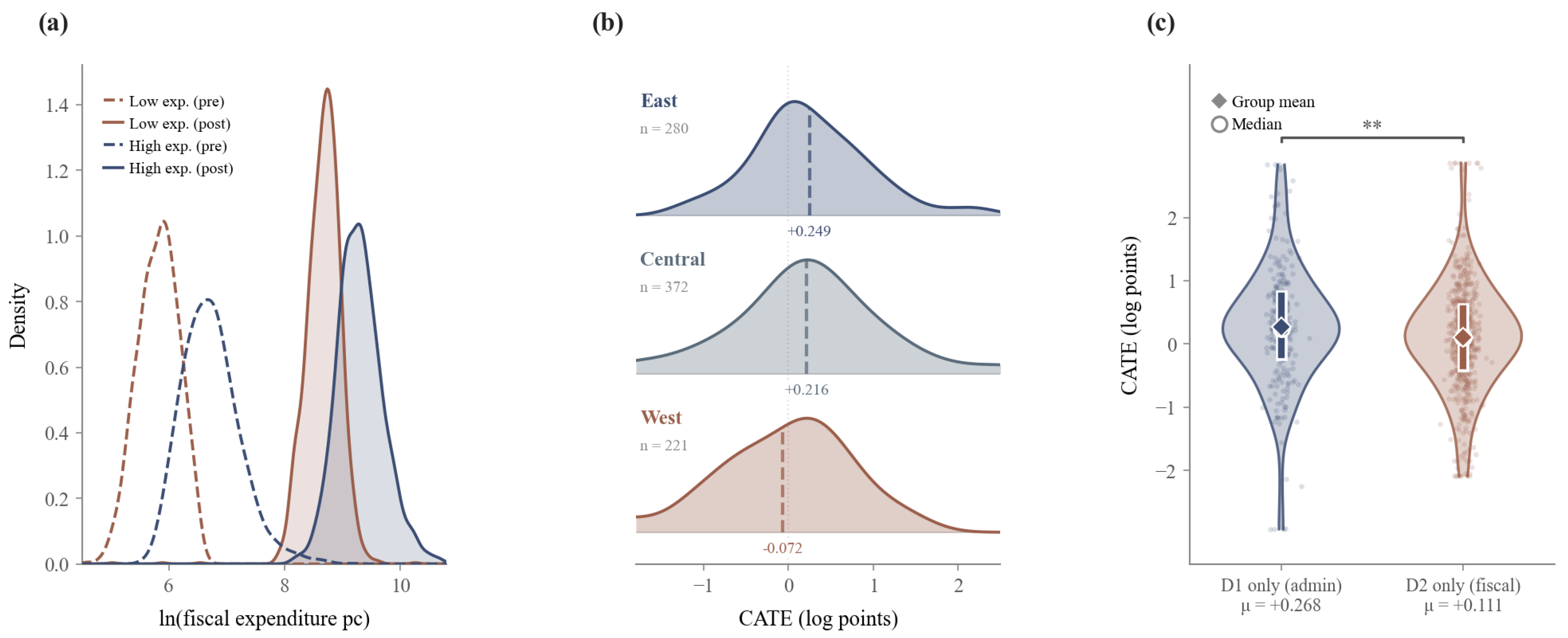
Figure 2c suggest that D1’s larger mean estimate comes mainly from a thicker upper tail. This pattern supports the systems hypothesis that decision-right architecture can matter for fiscal expenditure output, while remaining short of a definitive causal ranking of D1 and D2.
Fiscal direct reporting (D2) produces a positive but smaller effect (ATT = 0.103, 10.9% increase), statistically significant at the 10% level (). On the same baseline scale, this is roughly 66 yuan per capita at the mean baseline and 54 yuan at the median baseline. D2’s weaker effect may reflect the fact that rerouting fiscal accounting, while important for reducing prefecture interception of transfers, does not directly expand counties’ administrative decision space. Counties may receive modestly higher transfers but face similar approval bottlenecks in deploying those resources without accompanying administrative empowerment. The D2 estimate is also more heterogeneous, with the 95% CI spanning from effectively zero (−0.001) to 20.7%, suggesting that the effectiveness of D2 reform varies with local context.
The D1∩D2 row is retained only to document why no complementarity inference is possible. The group contains only treated counties in the estimation sample, all from Henan Province, and the estimate is statistically uninformative given the extremely wide confidence interval (95% CI: [−0.240, 0.356]). We do not generalize from this small cell and do not use it to infer whether D1 and D2 are complementary. Future work in provinces with larger simultaneous dual-reform rollouts could estimate the complementarity parameter more credibly. The D1 versus D2 differential is consistent with the interpretation that administrative decision authority may be a more important constraint than fiscal-flow channels for many county governments. Whether this institutional heterogeneity also maps onto China’s geographic landscape, where the uneven spatial distribution of reform types corresponds to big structural differences in regional governance capacity, is the question the following section addresses.
The regional diagnostics are consistent with the broader interpretation that institutional context conditions reform absorption, but they do not support a simple region-ranking conclusion. Panel fixed-effects estimates stratified by Eastern, Central, and Western China provide a descriptive within-county comparison. Western counties (
) show a larger descriptive association in the FE estimates (
, SE = 0.018,
), Eastern counties (
) show a smaller statistically significant positive association (
, SE = 0.016,
), and Central counties (
) show a near-zero association (
, SE = 0.012,
). These estimates are conditional correlations rather than regional counterfactual effects.
Table 10 reports the descriptive regional fixed-effects estimates.
To avoid relying only on region-specific FE benchmarks,
Table 11 summarizes county-level CATEs extracted from the common main gsynth model. This diagnostic uses the same fitted counterfactual structure for all treated counties. The common-model CATEs show positive median effects in all three regions, but the regional ranking differs from the FE comparison: Eastern and Central regions have larger mean CATEs than the Western region, while the Western region has a positive median but a negative mean because of a heavier lower tail. We therefore interpret the regional evidence as showing geographically uneven absorption of PMC reform, not as establishing that any one region has a robustly larger causal effect across all specifications.
This logic extends from geographic regions to the within-region expenditure distribution, where counties at the bottom of the expenditure spectrum may face a structural disadvantage in leveraging the new institutional framework. The unconditional quantile analysis examines this distributional pattern.
The aggregate regional pattern masks a within-distribution pattern with important implications for system performance. In the broader UQR sample, PMC reform is associated with larger estimated gains among counties near the middle and top of the expenditure distribution, while lower-tail effects are weak or negative. The panel unconditional quantile regression estimates no significant effect at Q10 (0.6%,
), a small negative effect at Q25 (
,
), and positive coefficients at Q50–Q90 (19.7% to 25.0%, all
). Because the UQR sample differs from the gsynth main sample, these estimates are interpreted as distributional evidence from a broader panel rather than as direct decompositions of the gsynth ATT.
Table 12 and
Figure 2a report the full panel UQR estimates.
The distributional results suggest a marked difference in reform incidence within the UQR sample. At Q10, the coefficient is near zero and statistically insignificant (0.006, ). At Q25, reform is associated with a small reduction in per-capita fiscal expenditure (ATT , ). From the median upward, reform is associated with positive effects: 25.0% at Q50, 24.5% at Q75, and 19.7% at Q90.
The distributional pattern therefore does not support a strong bottom-decile loss claim; instead, it supports the more cautious conclusion that lower-tail counties do not share the large gains observed above the median. Several mechanisms may account for this pattern. Provinces may couple PMC reform implementation with minimum public service standards, which can force low-capacity counties to reallocate budgets across categories. Fiscal direct reporting also requires counties to negotiate directly with provincial finance bureaus, a relationship that may disadvantage low-expenditure and typically rural counties with weaker administrative capacity. Finally, D2-only reform is more common among lower-expenditure counties, while D1 is more common among middle-range counties, contributing mechanically to weaker lower-tail estimates. These interpretations remain mechanisms to be investigated rather than fully identified pathways.
3.5. Mechanism Analysis
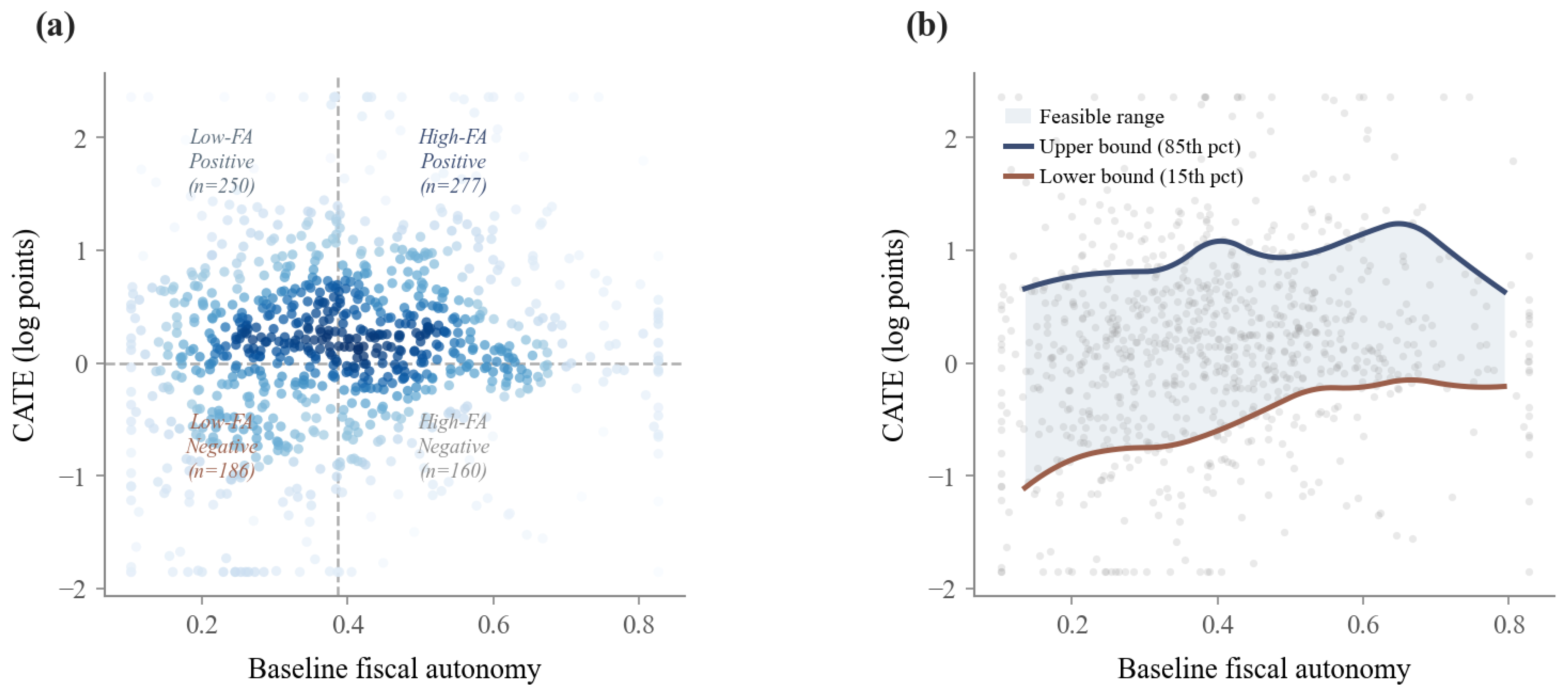
The positive aggregate effect and its spatial and distributional heterogeneity motivate an exploratory mechanism analysis of the fiscal autonomy channel. The estimates point to a counterintuitive denominator pattern in which reform is associated with higher total expenditure and a lower measured fiscal autonomy ratio, complicating conventional welfare interpretations of decentralization. These estimates represent descriptive conditional correlations rather than causal effects; county and year fixed effects partial out time-invariant confounders and common shocks but cannot fully address time-varying selection.
Table 13 presents the full results.
The relationship between reform and fiscal autonomy is documented in
Table 13, Column 1 is consistent with a denominator effect that is counterintuitive but mechanically plausible. Reform is associated with a reduction in fiscal autonomy of 3.2 percentage points (
). This pattern could arise if PMC reform increases counties’ total expenditure faster than own-source revenue, mechanically reducing the ratio of own revenue to total expenditure. This interpretation is related to the fiscal federalism literature on the flypaper effect, in which intergovernmental transfers “stick” to local fiscal expenditure instead of being fully offset by reductions in local revenue effort [
30]. It also differs from a pure substitution effect, under which added transfers would mainly replace own-source revenue without expanding total spending. In the PMC setting, a flypaper-style mechanism is plausible because D2 shortens the fiscal reporting path and can make provincial transfers more directly visible in county budgets. D1 can also increase counties’ ability to convert fiscal access into projects and services. The evidence in
Table 13 remains descriptive, however; it supports consistency with a transfer-driven expenditure channel rather than identifying that channel causally.
Figure 3 visualizes the fiscal-autonomy diagnostics underlying this mechanism discussion.
China’s 2016 VAT reform is relevant because it replaced the business tax with a value-added tax and changed the distribution of tax bases between central and local governments, potentially altering local own-source revenue and transfer dependence. To check whether the denominator pattern is driven by this national fiscal shock, we split the mechanism sample at 2016. The Reform → FA association is statistically significant in the pre-VAT period 2000–2015 (, SE = 0.005, ) and insignificant in the post-VAT period 2016–2019 (, SE = 0.048, ). The post-period null partly reflects the shorter four-year window and reduced reform variation post-2015; the pre-VAT result suggests that the denominator pattern is not solely a post-2016 artifact.
The second column of
Table 13 is consistent with a double-negative channel. Reform is associated with lower fiscal autonomy (
), and fiscal autonomy is negatively associated with expenditure (
). Counties with lower fiscal autonomy are more transfer-dependent and exhibit higher per-capita expenditure. One plausible explanation is that provincial transfers flow disproportionately to fiscally weaker counties to fund mandated services. The indirect association through the FA channel is positive but modest. The direct association between reform and expenditure conditional on FA is 0.037, and the combined panel-FE total is 0.043, substantially below the gsynth ATT of 0.154. This gap does not imply that the panel FE and gsynth estimates are inconsistent; they estimate different objects under different assumptions. Panel FE estimates the within-unit correlation between reform status and expenditure conditional on county and year fixed effects. By contrast, gsynth constructs the counterfactual of what expenditure would have been absent reform, accounting for time-varying unobservables that panel FE cannot absorb. The FA channel examined here represents one possible transmission pathway, not the complete explanation for the 16.7% preferred-specification expenditure increase. Other channels, including administrative empowerment effects on local investment and revenue mobilization, may contribute to the total gsynth ATT but lie outside the scope of the current mechanism analysis.
The third column tests the prefecture-level anchoring hypothesis with the variable city_control, defined as the inverse of the pre-reform variance in fiscal autonomy among non-reform counties within the same prefecture, where a higher value indicates a more fiscally homogeneous prefectural environment. The interaction between reform and this variable is negative and statistically insignificant (; SE = 0.000020; ). The negative sign is directionally consistent with the hypothesis that reform is more effective in prefectures where surrounding counties exhibit low fiscal variance, but the effect is economically tiny and statistically imprecise, reflecting the extreme right-skewness of city_control and limited within-prefecture variation in reform status. We retain this as an exploratory test while acknowledging that the current measurement strategy lacks sufficient precision for credible inference. These mechanism regressions provide exploratory evidence on one possible aggregate pathway, but they necessarily average over pronounced individual heterogeneity that the gsynth model makes visible through its full matrix of county-level treatment effects.
3.6. Spatial Diagnostics of Estimated Treatment Effects
The estimated treatment effects are consistent with spatial clustering, suggesting that weaker and stronger estimated gains may be geographically patterned rather than purely idiosyncratic. The county-level Conditional Average Treatment Effects (CATE) extracted from the main gsynth model exhibit substantial heterogeneity across the 873 treated counties.
Table 14 reports distributional statistics by reform type.
Three features of the CATE distribution suggest pronounced individual heterogeneity behind the aggregate ATT of 0.154. The unweighted post-treatment county mean (0.162) is close to the period-weighted ATT (0.154), suggesting that the average result is not driven solely by the weighting of early adopters. At the same time, the standard deviation (0.955) is large relative to the mean, indicating that county-level estimated effects are widely dispersed: the 10th percentile is −0.873 log points, while the 90th percentile is +1.121 log points. These tail estimates are generated quantities from the fitted gsynth model, so they should be interpreted as heterogeneity diagnostics rather than as precise county-level causal effects. The common model assigns positive estimated effects to all 10 D1∩D2 counties, but this Henan-only sample is too small for inference. The D1∩D2 CATE mean (0.527) also differs substantially from its separate four-group ATT in
Table 7 (0.058) because the two statistics originate from different model specifications. The CATEs in
Table 14 are extracted from the main combined-treatment model, which pools all 873 treated counties with
; the ATT in
Table 7 is estimated from a separate model with only 10 treated D1∩D2 units (
), where the counterfactual is less stable. We therefore do not draw inferential conclusions from either statistic for the D1∩D2 group.
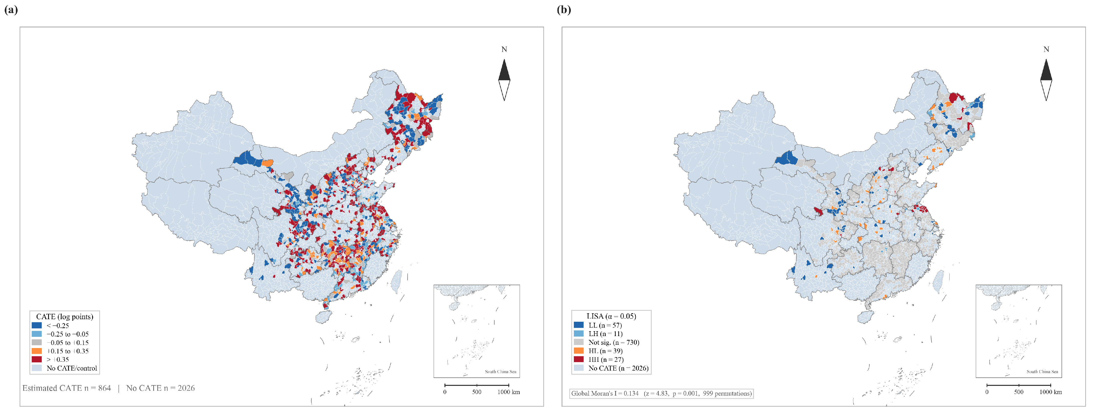
Exploratory spatial analysis of 864 estimated county-level post-treatment CATEs matched to the official standard-map service vector boundary base (map approval number: GS(2024)0650) is consistent with statistically significant geographic clustering (Global Moran’s , , ). Because CATEs are model-estimated quantities, these spatial statistics should be read as diagnostics of the geography of estimated effects rather than as observed spatial outcomes. The nine treated counties excluded from the spatial analysis reflect county-code or boundary-version mismatches in the official vector base and account for only 1.0% of treated counties. LISA identifies 27 High-High clusters, 57 Low-Low clusters, 39 High-Low spatial outliers, 11 Low-High spatial outliers, and 730 counties not significant at the 5% level. The presence of both Low-Low and High-Low locations suggests that weak or contrastive estimated effects are spatially structured, but the analysis remains exploratory.
Figure 4a indicates that high and low estimated CATEs are interspersed across the reforming county belt, with visible concentrations in Central, Southwestern, and Northeastern counties. Negative estimated CATEs appear in parts of Central China and the Northeast, indicating that positive regional medians in the common-model diagnostics can still mask higher and lower estimated effects within the same region. The LISA map in Panel (b) reports that both HH and LL clusters satisfy the 5% permutation threshold; this supports an exploratory interpretation that estimated treatment effects are spatially patterned.
The spatial evidence complements the heterogeneity analysis, while remaining exploratory. The reform-type estimates suggest that administrative power delegation may be more consequential than fiscal direct reporting; the regional diagnostics suggest that this logic varies geographically; the UQR results indicate that lower-expenditure counties benefit much less than counties above the median; and the LISA clusters suggest that weak estimated effects are spatially concentrated. A reform with a positive preferred-specification average effect may therefore still produce uneven estimated gains across the county system if low-gain counties share similar institutional and regional environments.