Case-Based-Reasoning Decision Method with Generalized Combination Rule

Abstract

Case-based reasoning (CBR) is an efficient intelligent decision-making approach, but traditional methods often neglect the weight and reliability of decision information and struggle with attribute heterogeneity and missing data. This study proposes a novel CBR method based on the generalized combination (GC) rule to overcome these limitations. We design differentiated similarity calculations for heterogeneous attributes, and construct basic probability assignments (BPAs) by grouping historical cases with identical similarity to handle missing data. Then, Deng entropy and Jousselme distance are used to characterize attribute weight and reliability, respectively. Discounted BPAs are recursively fused via the GC rule, and final decisions are derived through Bayesian approximation. A case study of typhoon disaster emergency decision-making demonstrates the superior performance of the proposed method.

1. Introduction

Case-based reasoning (CBR) is a decision-making method that offers distinct advantages by leveraging historical experience and analogical reasoning to address novel problems. Valued for its efficiency, interpretability, and ability to support continuous learning, CBR is widely applied in diverse domains, including medical diagnosis, legal adjudication, fault detection, and customer service. It has yielded measurable improvements, such as enhanced diagnostic accuracy, more consistent legal rulings, and faster resolution of technical faults, thus advancing intelligent decision-making across multiple sectors [1]. CBR continues to improve the efficiency and scientific robustness of decision-making processes with advancements in technologies such as big data, cloud computing, and artificial intelligence.

CBR is an intelligent approach that mimics human experiential decision-making. It constructs a repository of historical cases, uses similarity matching to find the most relevant precedents for a target problem, and then adapts and reapplies previous solutions to promote efficient decision-making. This process generally adheres to a four-stage iterative cycle, namely, “retrieval, reuse, revision, and retention,” which maintains decision efficiency and enables continuous learning. Current research on CBR mainly focuses on three key directions.

(1) CBR improvements based on similarity. Similarity-based improvement research typically uses classical or enhanced similarity calculation methods to identify and retrieve the most relevant cases from a case repository. Existing studies can be broadly categorized into two interconnected streams. The first research area focuses on refining similarity measurement methods for multidimensional data by developing better approaches to assess similarity across diverse attribute types, thereby improving reasoning effectiveness. Liao et al. [2] reviewed strategies for handling various attribute types and proposed a hybrid similarity measure that yielded satisfactory performance in fault diagnosis. Aamodt et al. [3] enhanced medical diagnostic accuracy by refining attribute-level similarity assessments and incorporating domain-specific knowledge. The second research stream focuses on optimizing weight calculation mechanisms within similarity metrics, aiming to systematically determine attribute weights and comprehensively integrate similarities across heterogeneous attributes. Hyung et al. [4] optimized weight allocation strategies to improve reasoning accuracy and reliability, while Cheng et al. [5] developed a dynamically adaptive weighting method that demonstrated strong practical efficacy. Núñez et al. [6] introduced an expert-guided weighting approach grounded in domain knowledge, offering valuable insights for CBR.

(2) Case repository management for CBR. Case repository management research focuses on establishing a scientifically grounded management system that covers the entire lifecycle of the repository, from storage and organization to maintenance and updating. This improves both retrieval efficiency and overall usability. Research in this domain can be divided into two streams. First, research on case indexing and retrieval optimization aims to enhance repository search performance using indexing techniques and advanced retrieval strategies. Sarkheyli et al. [7] applied a context operator model to case indexing, fuzzifying similar cases to optimize retrieval performance and streamline the repository structure. When applied to simulated driving scenarios, this method improved the efficiency of retrieving maneuvers such as overtaking. Similarly, Liu et al. [8] developed an ontology-based semantic case indexing system for equipment fault diagnosis, enabling multidimensional knowledge association. They increased cross-disciplinary case retrieval accuracy from 68% to 89%, supporting the diagnosis of complex faults, by constructing a semantic network linking fault phenomena to solutions. Second, studies on innovative repository construction and management methods aim to improve usability through systematic organization and governance mechanisms. For example, Guo et al. [9] integrated ontology techniques into CBR systems, combining dual ontology acquisition methods with novel semantic retrieval strategies to establish a more efficient case repository framework. When applied to injection mold design case management, this approach enabled engineers to accurately retrieve relevant cases, significantly improving design efficiency. Carmona et al. [10] proposed a novel system using CBR to help enterprises refine classification in key management areas, thereby enhancing management efficiency and resource-allocation precision. Further expanding the scope of repository management applications, Fu et al. [11] developed a multiagent system based on case reasoning for collaborative supply chain cost management.

(3) CBR integration with other technologies. Integrative research combines CBR’s experiential reuse capability with the strong points of other technological approaches. This enhances adaptability and precision in complex decision-making environments, mitigating the limitations of standalone CBR applications. Studies in this area mainly focus on (1) hybridization with rule-based reasoning, (2) integration with neural networks or fuzzy logic, and (3) fusion with emerging technologies. First, the integration of CBR with rule-based reasoning combines analogical inference with logical deduction, using rule-based constraints to narrow the case retrieval scope and improve reasoning efficiency. Saxena et al. [12], for example, combined both methods for automotive engine fault diagnosis. Here, rule-based reasoning first categorizes potential faults based on symptoms such as abnormal sounds or exhaust color, after which CBR retrieves and adapts historical repair cases to generate precise solutions, significantly enhancing diagnostic effectiveness. The second area of research incorporates neural networks or fuzzy logic into CBR, aiming to optimize similarity calculation and decision-making processes by leveraging machine learning capabilities or uncertainty modeling techniques. For example, Jang et al. [13] embedded neural networks and fuzzy logic in a CBR system for intelligent transportation. This approach dynamically learns from real-time traffic data and fuzzifies signal control rules, resulting in improved traffic throughput at intersections. Meanwhile, researchers have increasingly explored integrating CBR with emerging technologies such as text mining, Web 2.0, and artificial intelligence, thereby extending its applicability across diverse domains. Bun Foong et al. [14], for example, developed the Intelligent Help Desk Fault Management System, which integrates CBR with frame-based representation and employs text mining to automatically parse fault descriptions and match solutions, substantially reducing resolution time. Similarly, He [15] leveraged Web 2.0 technologies to construct a user feedback knowledge base integrated with CBR, improving product recommendation accuracy and user satisfaction. More recently, Zhang [16] drew upon case retrieval principles and hesitant fuzzy linguistic term sets (LTSs) to propose a view similarity-based freight-load matching method that incorporates shipper evaluations, thereby enhancing matching efficiency. In addition, the integration of CBR with deep learning and large language models (LLMs) has emerged as a new direction, for instance, in automatic feature extraction or similarity assessment [17,18,19,20]. These data-driven approaches are effective when large, complete datasets are available. However, in many real-world emergency decision-making scenarios, data are often sparse, incomplete, and heterogeneous, and interpretability is as critical as accuracy. Purely data-driven methods may lack robustness and transparency under such conditions. In contrast, our evidence–reasoning-based CBR/GC method is designed to handle high uncertainty, missing data, and attribute heterogeneity while providing interpretable outcomes through weight and reliability characterisation and the GC rule. Thus, the two paradigms are complementary, and our approach remains particularly suitable for emergency decision-making under imperfect information.

Existing studies have advanced CBR through three primary avenues: improvements in CBR based on similarity, case repository management for CBR, and the integration of CBR with other technologies. Such developments have enriched the theoretical foundations and modeling methods of CBR. In parallel, fuzzy multi-criteria decision-making (MCDM) methods have been widely applied to various real-world problems, such as shopping mall site selection [21], project selection under uncertainty [22], and competency ranking in education [23]. Nevertheless, while studies have accounted for typological differences among case attributes and integrated them through weighting strategies, they have largely overlooked the dimension of decision information reliability. This limitation undermines the precision of CBR outcomes. We propose that weight and reliability are two distinct dimensions of decision information. Weight reflects the relative importance of an attribute for solving a CBR problem: the more contributive a piece of information is to decision-making, the higher its weight should be. Reliability, by contrast, captures the accuracy or trustworthiness of decision information: the more accurate the information, the greater its reliability. Clearly, the scientific characterization and joint application of both weight and reliability are crucial for enhancing the effectiveness of CBR.

This study proposes a novel CBR decision-making method based on the generalized combination (GC) rule (hereafter, CBR/GC). This method not only characterizes the inherent properties of decision information through weight and reliability but also enables the integration of multidimensional decision information, thereby yielding more accurate and robust CBR outcomes. The method is structured as follows: first, to address the heterogeneity of attribute types, we introduce a tailored similarity measurement method to compare the target case with historical cases in the repository. By incorporating similarity classification and aggregation mechanisms, we develop a method for constructing the basic probability assignment (BPA) function. Second, each attribute is treated as an evidence source, represented by a BPA function. Drawing on Deng entropy and similarity measurement techniques, we establish both weight and reliability metrics for each evidence source, capturing the intrinsic and extrinsic characteristics of the decision information. Third, using the GC rule, evidence from all of the attribute-level sources associated with a given case is integrated, facilitating the identification of the most similar historical case and supporting subsequent decision-making.

Next, Section 2 presents the theoretical background, while Section 3 elaborates on the proposed CBR/GC-based decision-making method. Section 4 presents a comparative case study, and Section 5 presents the conclusions.

2. Preliminaries

2.1. Case-Based Reasoning

CBR is an empirical learning method that leverages historical cases through analogical reasoning and inference to solve new problems. It formalizes problems into target cases and historical cases, retrieving analogous instances from a historical repository [24]. By adapting solutions from retrieved cases, CBR provides actionable decision support for the target problem. The CBR process is commonly described as a “4R cycle,” consisting of four key stages: retrieval, reuse, revision, and retention:

(1) Retrieval. Abstract real-world problems into standardized target cases, then retrieve the most similar historical cases from the repository via similarity matching.

(2) Reuse. Reuse involves organizing historical cases using problem traits and domain knowledge to build a repository, where each becomes a potential source case for solutions.

(3) Revision. Evaluate and adjust the initial solution based on problem constraints, revising mismatches between historical cases and the current scenario.

(4) Retention. Store the validated target case and its effective solution in the repository to enable continuous learning of the system.

Retrieval is a critical component of CBR as it directly influences the effectiveness of subsequent stages. This study, therefore, focuses specifically on this phase, examining its methods and optimization strategies to improve the system’s overall performance and accuracy.

2.2. Similarity Calculation

In CBR, data on case attributes are generally classified into five types: symbolic, numerical, interval-valued, probabilistic, and ordinal. The symbolic type represents discrete, unordered categorical labels, whose values are used solely for classification and carry no numerical meaning. The numerical type consists of continuous or discrete quantitative data that support direct mathematical operations. The interval-valued type captures uncertainty in values through numerical ranges. The probabilistic type describes probability distributions over possible values, reflecting informational uncertainty. The ordinal type expresses clearly ordered hierarchical or gradational relationships, although it lacks equal intervals or additivity. Each attribute type requires distinct similarity measurement strategies to accurately assess case similarity. In this framework, the numerical type can be regarded as a special case of interval-valued data, while symbolic, probabilistic, and ordinal types can be uniformly represented as probabilistic LTS (PLTS) data.

Similarity calculation is a method for quantifying the degree of resemblance between different cases. Different attribute types require distinct similarity computation approaches. Specifically, interval-valued data are compared by measuring the distance between intervals, while PLTSs undergo structured adjustment to align their probabilistic distributions before an appropriate distance metric is applied. The resulting differences are then transformed into similarity values based on the inverse relationship between distance and similarity.

Definition 1

[25]. Let the attribute’s characteristic value be interval-valued data, with the target case’s attribute value represented as the interval and the comparison case’s attribute value represented as the interval. If the similarity between them is denoted by S, then it can be calculated using the following equation:

$$S=\exp (-{\displaystyle \frac{\sqrt{{\left({\tilde{x}}^{+}-x^{+}\right)}^2+{\left({\tilde{x}}^{-}-x^{-}\right)}^2}}{\arg {\max }_m\left\{\sqrt{{\left({\tilde{x}}^{+}-x^{+}\right)}^2+{\left({\tilde{x}}^{-}-x^{-}\right)}^2}\right\}}})$$

(1)

where arg max denotes the parameter that maximizes the value of the i-th attribute x across all historical cases, specifically referring to the maximum value itself. Meanwhile, exp represents the exponential function with base e. This procedure converts the original distance interval into a normalized similarity measure, thus facilitating the quantitative assessment of similarity for interval-type attributes.

Interval-valued attribute values require the consideration of both upper and lower bounds. Therefore, calculations incorporate the midpoint and interval width. Similarity values range from 0 to 1, with smaller differences indicating greater similarity. Consequently, the Euclidean distance is used to measure these differences, which are then normalized to the [0, 1] range using min-max normalization.

Specifically, when interval-type attribute values contain missing data, no numerical imputation is applied. Instead, the missing attribute is represented as an aggregated interval derived from the upper and lower bounds of all of the available historical cases for that attribute, with subsequent computations based on this constructed interval.

For the PLTS data, calculations are conducted in accordance with Definitions 2–4. The probability distributions are first adjusted by rearranging their probabilistic components according to a specified rule to achieve structural consistency. Similarity is then computed using the Hamming distance metric.

Definition 2

[26]. Let $S=\{s_a|a=-\tau ,\cdots ,-\mathsf{1},\mathsf{0},\mathsf{1},\cdots ,\tau \}$ denote an LTS and ${\widehat{h}}_S^1(p)=\{s_a^{1(l)}({\widehat{p}}^{1(l)})|$$l=1,2,\cdots ,L_1\}$ and ${\widehat{h}}_S^2(p)=\{s_{\alpha }^{2(l)}({\widehat{p}}^{2(l)})|l=1,2,\cdots ,L_2\}$ denote two normalized PLTSs. Suppose ${\widehat{h}}_S^1(p)$ and ${\widehat{h}}_S^2(p)$ yield the rearranged probability sets $P={\{p^{\ast (1)},p^{\ast (2)},\cdots ,p^{\ast (K)}\}}^T$. The structure is made consistent by supplementing linguistic terms with zero probability, resulting in adjusted PLTS $h_S^{\ast 1}(p)=\{s_{\alpha }^{1(k)}(p^{\ast (k)})|k=1,2,\cdots ,K\}$ and $h_S^{\ast 2}(p)=\{s_{\alpha }^{2(k)}(p^{\ast (k)})|k=1,2,\cdots ,K\}$, where the following conditions hold:

• $p^{\ast (1)}:=\min \{{\widehat{p}}^{11},{\widehat{p}}^{21}\}$;
• If $p^{\ast (1)}={\widehat{p}}^{11}, p^{\ast (2)}:=\min \{{\widehat{p}}^{12},{\widehat{p}}^{21}-p^{\ast (1)}\}$;
• If $p^{\ast (1)}={\widehat{p}}^{21}, p^{\ast (2)}:=\min \{{\widehat{p}}^{22},{\widehat{p}}^{11}-p^{\ast (1)}\}$;
• If $p^{\ast (1)}={\widehat{p}}^{11}$ and $p^{\ast (2)}={\widehat{p}}^{12}$, $p^{\ast (3)}:=\min \{{\widehat{p}}^{13},{\widehat{p}}^{21}-p^{\ast (1)}-p^{\ast (2)}\}$;
• If $p^{\ast (1)}={\widehat{p}}^{11}$ and $p^{\ast (2)}={\widehat{p}}^{21}-p^{\ast (1)}$, $p^{\ast (3)}:=\min \{{\widehat{p}}^{12}-p^{\ast (2)},{\widehat{p}}^{22}\}$;
• If $p^{\ast (1)}={\widehat{p}}^{21}$ and $p^{\ast (2)}={\widehat{p}}^{22}$, $p^{\ast (3)}:=\min \{{\widehat{p}}^{23},{\widehat{p}}^{22}-p^{\ast (1)}-p^{\ast (2)}\}$;
• If $p^{\ast (1)}={\widehat{p}}^{21}$ and ${\widehat{p}}^{11}-p^{\ast (1)}$, $p^{\ast (3)}:=\min \{{\widehat{p}}^{22}-p^{\ast (2)},{\widehat{p}}^{12}\} ,\cdots , p^{\ast (K)}$.

${\widehat{p}}^{1(l)}=p^{\ast (k)}+p^{\ast (k+1)}+\cdots +p^{\ast (k+h)}$ must hold, where ${\widehat{p}}^{1(l)}$ is the probability of $s_{\alpha }^{1(l)}$ within the element in ${\widehat{h}}_s^1(p)$. h denotes the number of language terms in $h_S^{\ast 1}(p)$ (elements in $h_S^{\ast 2}(p)$ also satisfy this condition). In the adjusted probability language expectations, the sum of the language terms and their probabilities remains unchanged.

Definition 3

[26]. Let $S=\{s_{\alpha }|\alpha =$$-\tau ,\cdots ,-1,0,1,\cdots ,\tau \}$ denote an LTS. For two normalized probabilistic linguistic elements ${\widehat{h}}_S^1(p)$ and ${\widehat{h}}_S^2(p)$ on S, assuming their adjusted forms are $h_S^{\ast 1}(p)=\{s_{\alpha }^{1(k)}(p^{\ast (k)})|$$k=1,2,\cdots ,K\}$ and $h_S^{\ast 2}(p)=\{s_{\alpha }^{2(k)}(p^{\ast (k)})|k=1,2,\cdots ,K\}$, respectively, the Hamming distance between $h_S^{\ast 1}(p)$ and $h_S^{\ast 2}(p)$ can be defined as

$$d_{h,d}\left({\widehat{h}}_S^1(p),{\widehat{h}}_S^2(p)\right)={\displaystyle \sum _{k=1}^K{p}^{\ast (k)}}{\displaystyle \frac{\left|{\alpha }^{1(k)}-{\alpha }^{2(k)}\right|}{2\tau }},$$

(2)

where ${\alpha }^{1(k)}$ and ${\alpha }^{2(k)}$ denote the indices of linguistic terms, and $\tau$ represents the maximum index of the LTS.

Definition 4

[26]. Let the attribute values be PLTS data. For two normalized probabilistic linguistic elements ${\widehat{h}}_S^1(p)$ and ${\widehat{h}}_S^2(p)$, their similarity is defined as $\rho \left({\widehat{h}}_S^1(p),{\widehat{h}}_S^2(p)\right)$, denoted as S.

$$S=\rho \left({\widehat{h}}_S^1(p),{\widehat{h}}_S^2(p)\right)=1-d\left({\widehat{h}}_S^1(p),{\widehat{h}}_S^2(p)\right)$$

(3)

Example 1.

Let $S=\{s_{-3},s_{-2,}\cdots ,s_3\}$ with $\tau =3$. Consider two normalized PLEs ${\widehat{h}}_1(p)=\{s_1(0.6),s_2(0.4)\}$ and ${\widehat{h}}_2(p)=\{s_0(0.3),s_1(0.7)\}$. Following the adjustment procedure in Definition 2, we align their probability sets. The adjusted forms are $h_1^{\ast }(p)=\{s_1(0.3),s_1(0.3),s_2(0.4)\}$ and $h_2^{\ast }(p)=\{s_0(0.3),s_1(0.3),s_1(0.4)\}$, with probability blocks $p^{\ast }(1)=0.3$, $p^{\ast }(2)=0.3$, $p^{\ast }(3)=0.4$. The corresponding linguistic indices for each block are $(1,0)$, $(1,1)$, and $(2,1)$. Using Definition 3, the Hamming distance is $d=0.3\ast \left|1-0\right|/2\tau +0.3\ast \left|1-1\right|/2\tau +0.4\ast \left|2-1\right|/2\tau \approx 0.1167$. Finally, by Definition 4, the similarity is $S=1-d\approx 0.8833$. This example illustrates the adjustment process and the distance computation.

Specifically, when PLTS attribute values contain missing data, the equal probability allocation method is applied. This procedure first assigns identical probabilities to all of the linguistic terms in the set, ensuring that the total probability sums to unity, after which calculations proceed according to Definitions 2–4.

2.3. GC Rule

The GC rule is a synthetic approach grounded in evidential reasoning (ER) and Dempster–Shafer (DS) evidential theory. It addresses the inherent limitations of ER methods by introducing a universal discounting method that accounts for both evidence weight and reliability characteristics. Reliability is treated as an intrinsic property of evidence for discounting purposes, with residual support from weights allocated to power sets. Subsequently, the discounted evidence is combined via orthogonal sum operations, culminating in decision-making under specified principles.

Definition 5

[27]. Let a possible hypothesis of a variable be ${\theta }_n(n=1,2,\cdots ,N)$, and each of the possible hypotheses is exclusive. A finite nonempty exhaustive set of all of the possible hypotheses $\Theta =\{{\theta }_1,{\theta }_2\cdots ,{\theta }_N\}$ is called a frame of discernment, and its power set consisting of 2^N subsets of Θ is usually expressed as follows:

$$P(\Theta )=\{\varnothing ,{\theta }_1,\cdots ,{\theta }_N,\{{\theta }_1,{\theta }_2\},\cdots ,\{{\theta }_1,{\theta }_N\},\cdots , \{{\theta }_1,\cdots ,{\theta }_{N-1}\},\Theta \}$$

(4)

Definition 6

[27]. Let $(\theta ,p_{\theta ,i})$ denote that the evidence $e_i$ points to proposition $\theta$ to belief degree $p_{\theta ,i}$. The profiled expression is called the belief distribution (BD) of $e_i$.

$$b_i=\{(\theta ,p_{\theta ,i}),\forall \theta \subseteq \Theta ,{\displaystyle \sum _{\theta \subseteq \Theta }{p}_{\theta ,i}}=1\}$$

(5)

Definition 7

[28]. Let $m_1$ and $m_2$ be two pieces of evidence. They are in the same frame of discernment Θ, which contains N mutually exclusive and exhaustive hypotheses. The Jousselme distance between $m_1$ and $m_2$ can be defined as follows:

$$J=\sqrt{{\displaystyle \frac{1}{2}}{({\overrightarrow{m}}_1-{\overrightarrow{m}}_2)}^T D({\overrightarrow{m}}_1-{\overrightarrow{m}}_2)}$$

(6)

Definition 8

[29]. Let $w_i$ be the weight of evidence $e_i$, with $r_i =0$. $r_i$ is the reliability of $e_i$, with $0\leqq r_i\leqq 1$, where $r_i =0$ corresponds to “completely unreliable” and $r_i=1$ corresponds to “completely reliable.” The basic probability mass for $e_i$, discounted by both weight and reliability, is then assigned as follows:

$$m_{\theta ,i}=m_i(\theta )=\left\{\begin{array}{ll}0\hfill & \theta =\varnothing \hfill \\ w_i{r}_i{p}_{\theta ,i}\hfill & \theta \subset \Theta \hfill \\ w_i{r}_i{p}_{\theta ,i}+w_i(1-r_i)\hfill & \theta =\Theta \hfill \\ 1-w_i\hfill & \theta =P(\Theta )\hfill \end{array}\right.$$

(7)

Definition 9

[29]. Let there be I pieces of independent evidence to be combined, and let $e_i$ be the i-th piece of evidence with weight $w_i$ and reliability $r_i$, $i=1,2,\cdots ,I$. The BD of $e_i$ is profiled by Equation (5) and discounted by Equation (7) $e_i$ is the combination of the first i pieces of evidence, and its combined probability mass is $m_{\theta ,e(i)}$, with $m_{\theta ,e(1)}=m_{\theta ,1}$ and $m_{P(\Theta ),e(1)}=m_{P(\Theta ),1}$. The orthogonal sum of the first i discounted probability masses is then determined by

$$m_{\theta ,e(i)}=[m_1\oplus \cdots \oplus m_i](\theta )=\left\{\begin{array}{ll}0\hfill & \theta =\varnothing \hfill \\ {\displaystyle \frac{{\widehat{m}}_{\theta ,e(i)}}{{\displaystyle \sum _{\vartheta \subseteq \Theta }{\widehat{m}}_{\vartheta ,e(i)}}+{\widehat{m}}_{P(\Theta ),e(i)}}}\hfill & \theta \ne \varnothing \hfill \end{array}\right.$$

(8)

$${\widehat{m}}_{\theta ,e(i)}=\left[{\displaystyle \sum _{B\cap C=\varnothing ,B,C\subseteq \Theta }{m}_{B,e(i-1)}}{m}_{C,i}+m_{\theta ,e(i-1)}{m}_{\Theta ,i}+m_{\theta ,i}{m}_{\Theta ,e(i-1)}\right]+\left[(1-w_i)m_{P(\Theta ),e(i-1)}{m}_{\theta ,i}\right],\theta \subset \Theta$$

(9)

$${\widehat{m}}_{\Theta ,e(i)}=m_{\Theta ,e(i-1)}{m}_{\Theta ,i}+\left[m_{P(\Theta ),e(i-1)}{m}_{\Theta ,i}+(1-w_i)m_{\Theta ,e(i-1)}\right]$$

(10)

$${\widehat{m}}_{P(\Theta ),e(i)}=(1-w_i)m_{P(\Theta ),e(i-1)}$$

(11)

Definition 10

[29]. The combined BDs of I pieces of independent evidence are determined by

$$p_{\theta }=p_{\theta ,e(I)}=\left\{\begin{array}{ll}0\hfill & \theta =\varnothing \hfill \\ {\displaystyle \frac{{\stackrel{⌢}{m}}_{\theta ,e(I)}}{{\displaystyle \sum _{\theta \subseteq \Theta }{\stackrel{⌢}{m}}_{\theta ,e(I)}}}}\hfill & \theta \subseteq \Theta ,\theta \ne \varnothing \hfill \end{array}\right.$$

(12)

where ${\widehat{m}}_{\theta ,e(I)}$ is calculated using Equations (9) and (10) for $i=I$, $0\le p_{\theta ,e(I)}\le 1$ for $\theta \subseteq \Theta$, and ${\displaystyle {\sum }_{\theta \subseteq \Theta }{p}_{\theta ,e(I)}}=1$.

Definition 11

[30]. In the evidence theory framework, the combined belief distribution may contain both local and global ignorance, making it unsuitable for direct decision-making. To support decision-making, a Bayesian approximation is applied to convert the BPA into a probability distribution over single-element propositions. For each hypothesis ${\theta }_n\in \Theta$, the approximated BPA is defined as

$$\overline{m}({\theta }_n)=\left\{\begin{array}{l}{\displaystyle \frac{{\displaystyle {\sum }_{A\subseteq \Theta ,{\theta }_n\in A}m(A)}}{{\displaystyle {\sum }_{A\subseteq \Theta }m(A)·\left|A\right|}}},\forall n\\ 0,\mathrm{others}\end{array}\right.$$

(13)

3. Proposed Method

3.1. Modeling Framework

The main objective of CBR decision-making is to derive efficient solutions for target problems through the similarity-based matching of historical cases and evidence fusion. This section presents a CBR decision-making framework based on the GC rule (CBR/GC), whose fundamental principle involves optimizing the evidence-fusion process by integrating both weight and reliability considerations. This approach mitigates the decision biases inherent in traditional methods, which often stem from neglecting variations in information quality and importance.

A case may be formally described as $(P,S,R)$, where P denotes the problem description, S represents the solution to the problem, and R denotes the solution outcome. The case base, comprising historical cases analogous to the target case, can be represented as $C=\{c_l|l=1,2,\cdots ,L\}$, where L signifies the number of cases in this base.

In CBR, the problem description P typically comprises a set of attributes that collectively characterize the case scenario. The case attributes used in this study constitute the problem attributes that form the problem description P. During the case retrieval phase, these attributes are employed to match similar cases and identify analogous scenario contexts. For example, in the typhoon case, attributes such as “typhoon type” and “central pressure” are used to retrieve similar historical cases. A case attribute may be denoted as F, with the attribute sets defined as $F_n=\{f_{i_n}|i_n=1,2,\cdots ,i_N\},n=1,\cdots ,5$ and $I_1+\cdots +I_5=I$. Any attribute can be represented as $f_i(i=1,2,\cdots ,I)$, where $F_1$–$F_5$ denote symbolic, numerical, interval, probabilistic, and ordinal attributes, respectively, satisfying $F_x\cap F_y=\Phi (x,y=1,2,3,4,5;x\ne y)$ and $F_x\cup F_y=F$. For the l-th case $c_l$, the performance value on the i-th problem attribute $f_i$ is denoted as $x_i^l$, where $l=1,2,\cdots ,L$ and $i=1,2,\cdots ,I$. Then, the problem description P can be expressed as a vector of the values of each attribute $P=(x_1,x_2,\cdots ,x_I)$, where $x_i$ is the value of the case on the i-th attribute. The original case base C can thus be represented as shown in

Table 1. Composition of the Original Case Base.

Case	Attribute 1	Attribute 2	…	Attribute I
c1	${\mathrm{x}}_1^1$	${\mathrm{x}}_2^1$	…	${\mathrm{x}}_{\mathrm{I}}^1$
c2	${\mathrm{x}}_1^2$	${\mathrm{x}}_2^2$	…	${\mathrm{x}}_{\mathrm{I}}^2$
…	…	…	…	…
cL	${\mathrm{x}}_1^{\mathrm{L}}$	${\mathrm{x}}_2^{\mathrm{L}}$	…	${\mathrm{x}}_{\mathrm{I}}^{\mathrm{L}}$

Note: The ellipsis (…) indicates that some intermediate rows or columns are omitted due to space limitations. L denotes the case index. Intermediate rows are omitted due to space limitations.

.

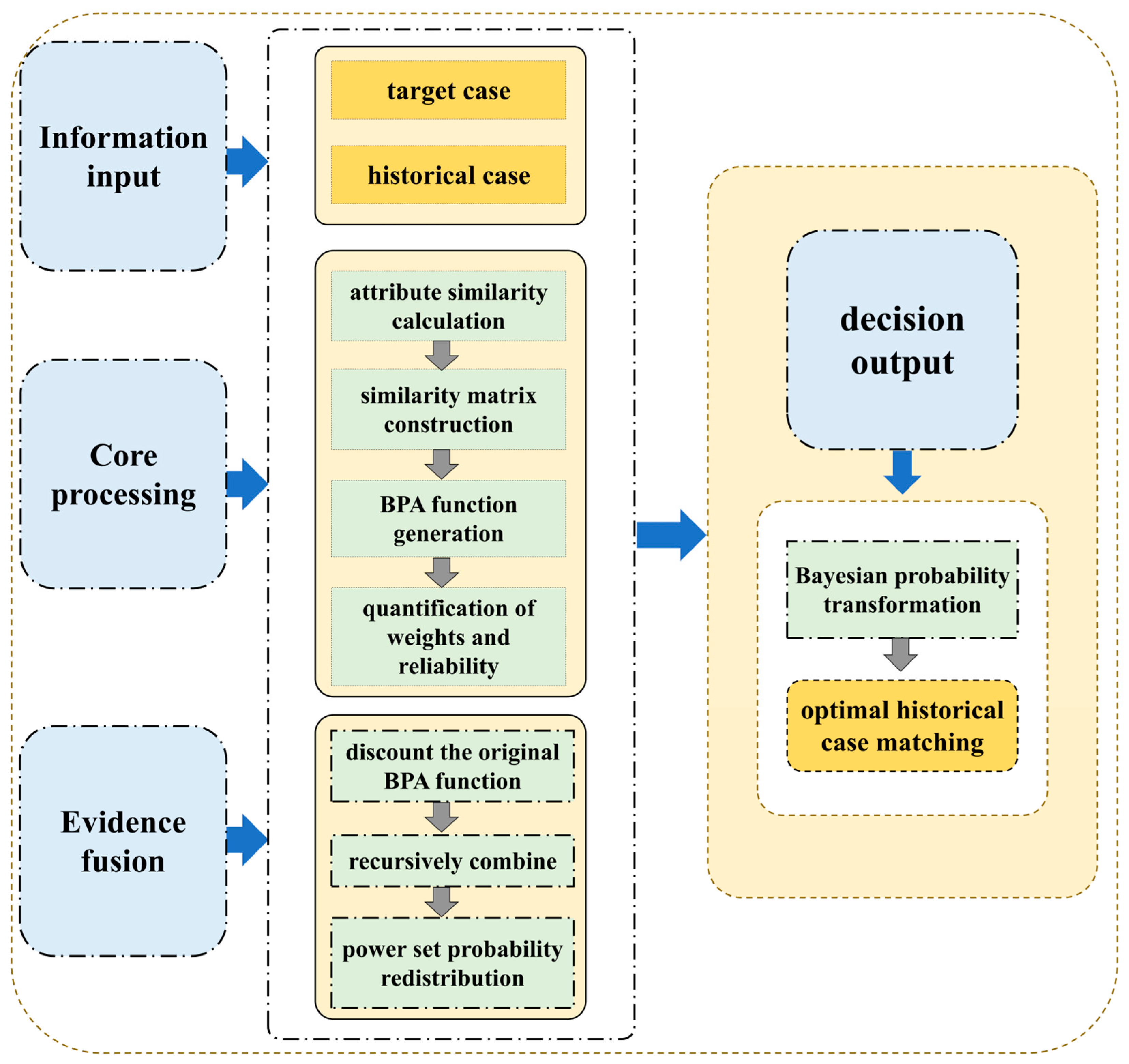
Existing case retrieval methods are limited in several ways. They often fail to adequately account for attribute heterogeneity and interactions, and during evidence fusion, they neglect both the objective quality (reliability) and subjective importance (weighting) of information. These limitations result in biased reasoning outcomes and compromised decision accuracy. To address these issues, we propose a novel framework that improves the accuracy and effectiveness of CBR, thereby enhancing its applicability to real-world decision-making scenarios. To better illustrate the interactions among the four core components of the proposed CBR/GC method, we first describe the logical flow. Similarity calculation is performed for each attribute of the target case against all historical cases, yielding a matrix of local similarity values. These similarity values are then grouped by identical scores to construct a BPA for each attribute, which serves as the evidential input. From each BPA, two quality indicators are derived. The weight is calculated via Deng entropy to reflect the attribute’s discriminative uncertainty, while the reliability is obtained via Jousselme distance to measure the attribute’s consistency with others. The original BPA is then discounted using both weight and reliability, where a lower reliability reduces the contribution of that piece of evidence. All discounted BPAs are subsequently fused by the GC rule through recursive orthogonal summation. Finally, the fused belief distribution is transformed into Bayesian probabilities to rank the historical cases and identify the most similar match. This stepwise interaction is also visualised in Figure 1. To this end, we propose the following framework (Figure 1):

Similarity measure. Similarity measures are first employed to evaluate the correspondence between the target case and historical cases with respect to each attribute. Based on these similarity measures, all of the historical cases are used to construct the frame of discernment, within which a BPA function is defined for each individual attribute.

Weight and reliability calculation. The BPA function corresponding to each attribute is considered as a piece of evidence reflecting potential alignment between historical cases and the resolution of the target case. The weight and reliability of each piece of evidence are subsequently calculated using methods such as Deng entropy.

Evidence fusion. All of the evidence information, along with the corresponding weights and reliability, is combined using the GC rule to support subsequent decision-making.

3.2. Similarity-Based Determination of the BPA Function

In the CBR framework, determining the BPA function plays a crucial role, as it directly affects the accuracy and effectiveness of the reasoning process. This function is closely tied to the diversity of case attributes; it has implications for overcoming traditional case retrieval challenges and enabling effective evidence fusion. Constructing the BPA function in CBR involves establishing BPA functions through customized similarity calculation strategies that account for various attribute types. This approach precisely captures the similarity relationships between cases and provides a robust foundation for subsequent evidence combination.

In local similarity computation, it is common for multiple historical cases to exhibit identical similarity values with respect to the target case under a given attribute. Traditional case retrieval methods often address this scenario inadequately before proceeding to global similarity aggregation. They typically resort to simplistic strategies such as averaging attribute values or random selection. Such approaches may lead to inaccurate case ranking within the repository [25]. For example, in earthquake emergency resource decision-making, the “magnitude” attribute of a target case may match several historical cases equally, rendering retrieval outcomes based solely on this attribute insufficient for meaningful differentiation. To address this limitation, we model historical cases with identical local similarity values as concurrent and indistinguishable propositions, thereby transforming the local similarity results into a BPA function.

We posit that the core of case reasoning lies in analogy based on historical cases; hence, the frame of discernment should encompass all of the available historical cases. Treating each case as a potential solution, the system can identify the most similar cases when addressing new problems, thereby reusing their solutions. Consequently, the frame of discernment studied here can be represented as $C=\{c_1,\cdots ,c_l,\cdots ,c_L\}$, where the element $c_l$ represents the l-th historical case, and $l=1,2,\cdots ,L$.

As discussed in Section 2.2, existing studies classify attribute data into five types: symbolic, numerical, interval, probabilistic, and ordinal. Two observations are worth noting: (1) numerical types can be regarded as a special case of interval types in which the upper and lower interval bounds are identical. Therefore, we integrate numerical and interval types into a unified category referred to as interval-type attributes, denoted as K₁. (2) Symbolic, probabilistic, and ordinal types can all be transformed into PLTS, characterized by combining linguistic scales with probability distributions. Accordingly, these are grouped together in this study as PLTS-type attributes, denoted as K₂.

Example 2.

For the attribute “typhoon type”, define an LST $S=\{s_1:Tropical Storm,s_2:Severe Tropical storm,s_3:Typhoon\}$. A case record “Tropical Storm” is converted to the PLTS $\{S_1(1)\}$; “Typhoon” becomes $\{S_3(1)\}$, etc. This provides a deterministic mapping from each original value to a single-term PLTS.

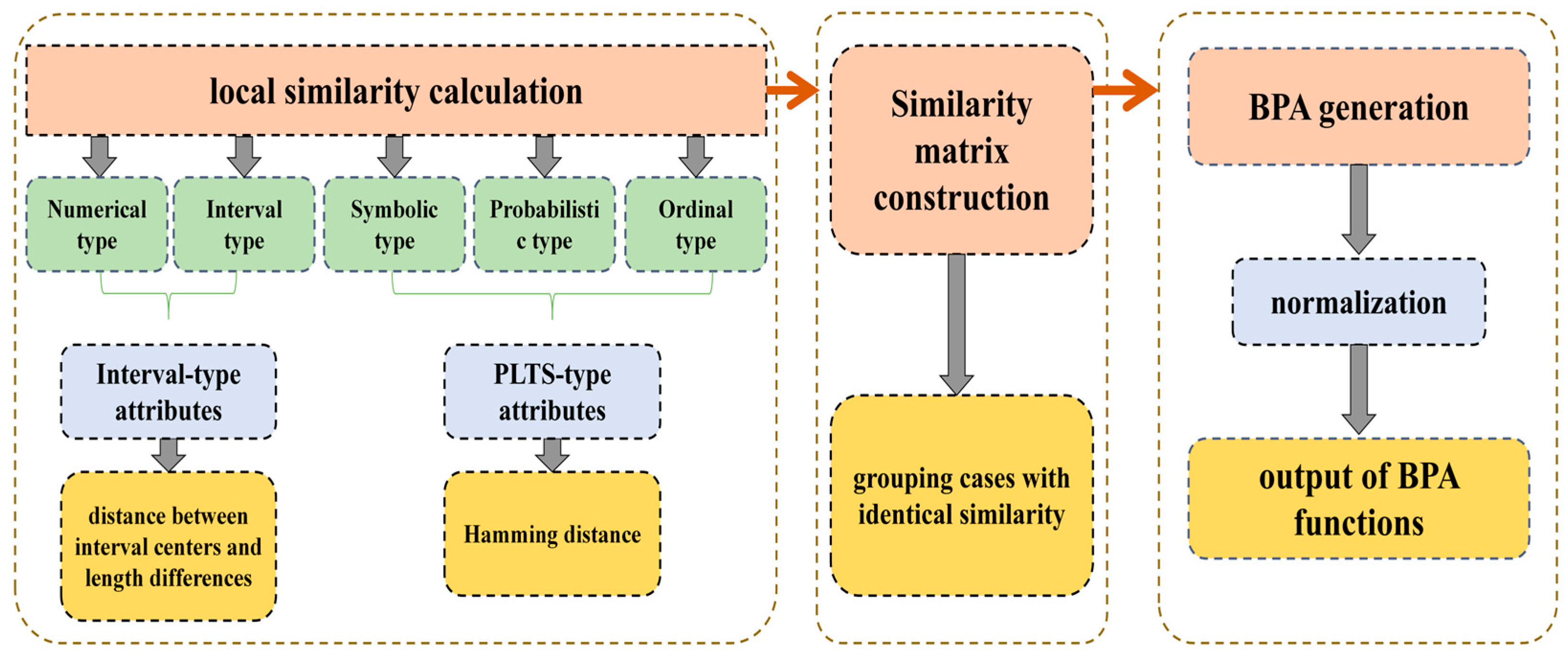
The specific calculation steps are as follows (Figure 2):

Step 1: Calculate local similarity according to Definitions 1–4. During the case retrieval phase, we utilize attributes to compute the similarity between the target case $\tilde{c}$ and historical case $c_l$ for each attribute across different types.

When calculating local similarity for an interval-type attribute $f_i$, the target case $\tilde{c}$ has an interval $\left[{\tilde{x}}_i^{-}\right.,\left.{\tilde{x}}_i^{+}\right]$ on the interval-type attribute $f_i$, while the historical case $c_l$ has an interval $\left[x_i^{l-}\right.,\left.x_i^{l+}\right]$. Similarity is computed $s_i^l$ by combining the distance between interval centers and the difference in interval lengths. The similarity value falls in the interval $\left[0\right.,\left.1\right]$. The Euclidean distance quantifies the positional and length differences between intervals; smaller differences yield higher similarity. According to Definition 1, the local similarity between the target case $\tilde{c}$ and the historical case $c_l$ under interval-type attributes can be expressed as follows:

$$s_i^l=\exp (-{\displaystyle \frac{\sqrt{{\left({\tilde{x}}_i^{+}-x_i^{l+}\right)}^2+{\left({\tilde{x}}_i^{-}-x_i^{l-}\right)}^2}}{\arg {\max }_l\left\{\sqrt{{\left({\tilde{x}}_i^{+}-x_i^{l+}\right)}^2+{\left({\tilde{x}}_i^{-}-x_i^{l-}\right)}^2}\right\}}}), i=1,2,\cdots ,I;l=1,2,\cdots ,L$$

(14)

When calculating local similarity for a PLTS-type attribute $f_i$, probabilities are first rearranged according to the specific rule in Definition 2 to align the probability set structure. Similarity is then computed using the Hamming distance equation. Based on Definitions 3 and 4, the similarity calculation between the target case $\tilde{c}$ and historical case $c_l$ for attribute $f_i$ is expressed as follows:

$$s_i^l=\rho \left({\widehat{h}}_S^1(p),{\widehat{h}}_S^2(p)\right)=1-d\left({\widehat{h}}_S^1(p),{\widehat{h}}_S^2(p)\right)$$

(15)

We address the challenges of missing and heterogeneous attribute values by transforming similarity measures into BPAs. When attribute values are missing, they are not subjected to forced imputation. Instead, a BPA is constructed for the affected attribute, thereby indirectly representing the uncertainty in similarity assessment. This approach avoids the biases associated with traditional interpolation methods and provides a more robust way to handle missing data.

Step 2: For each attribute, following the aforementioned similarity calculation, the resulting similarity values are organized into a similarity matrix:

$$\begin{array}{l}\begin{array}{c}\hspace{1em}\hspace{1em} f_1 \cdots f_i \cdots f_I\end{array}\\ \tilde{s}=\begin{array}{c}{c}_1\\ ⋮\\ c_l\\ ⋮\\ c_L\end{array}\left[\begin{array}{cccc}{s}_1^1& s_i^1& \cdots & s_I^1\\ ⋮& ⋮& \ddots & ⋮\\ s_1^l& s_i^l& \cdots & s_I^l\\ ⋮& ⋮& \ddots & ⋮\\ s_1^L& s_i^L& \cdots & s_I^L\end{array}\right]\end{array}$$

Here, rows represent historical cases $c_l(l=1,2,\cdots ,L)$, columns denote attribute $f_i(i=1,2,\cdots ,I)$, and the matrix content $s_i^l$ indicates the similarity value between the target case $\tilde{c}$ and a historical case $c_l$ under attribute $f_i$.

The similarity matrix quantifies the degree of similarity between the target case and all of the historical cases across various attributes. Through differentiated calculations, it uniformly transforms different attribute types into similarity values within the interval [0, 1], enabling the integration of heterogeneous attributes. This supports cross-attribute comparisons and establishes a solid data foundation for subsequent case retrieval and matching.

Step 3: Convert local similarity $s_i^l$ into the BPA function.

Traditional case retrieval methods assume a complete case base. When attribute values are missing, prior to similarity calculation, data are typically imputed using techniques such as interpolation or mean imputation. However, this approach has two main limitations: imputed values may deviate from the true values, thereby introducing bias into similarity assessments. Moreover, the inherent uncertainty associated with missing values (e.g., “unknown,” “unrecorded”) is often inadequately captured, which compromises the accuracy of case matching.

Definition 12.

Let $s_i^l$ denote the similarity between target case $\tilde{c}$ and historical case $c_l$ on attribute $f_i$, where $l=1,2,\cdots ,L$. Sort all of the historical cases by similarity in descending order. Historical cases with identical similarity values are grouped into the same rank category, with rank categories ${\theta }_i^n$ defined, where $n=1,2,\cdots ,N_i$. The similarity $S_i^n$ between the n-th rank category ${\theta }_i^n$ on attribute $f_i$ and target case can be represented by the similarity of its constituent historical cases; that is, $S_i^n=s_i^l$, $c_l\in {\theta }_i^n$.

Definition 13.

Let the similarity between the target case $\tilde{c}$ and the rating category ${\theta }_i^n$ on the attribute $f_i$ be denoted as $S_i^n$, and let the historical cases contained within the rating category be denoted as ${\theta }_i^n=(c_{i·n}^l|l=1,2,\cdots ,L_n)$. If the frame of discernment is set as the set of all historical cases $\Theta =(c_l|l=1,2,\cdots ,L)$, then the fundamental probability distribution function for the rating category ${\theta }_i^n$ can be computed using the following equation:

$$b({\theta }_i^n)=S_i^n/{\displaystyle {\sum }_n{S}_i^n},n=1,2,\cdots ,N, i=1,2,\cdots ,I$$

(16)

(1)

When considering a single subset in the frame of discernment (the set comprising the target case $\tilde{c}$ and its uniquely matched historical case), if the similarity between the target case $\tilde{c}$ and the historical case $c_l$ under attribute $f_i$ is $s_i^l$, and the target case $\tilde{c}$ and the historical case $c_l$ possess unique similarity under attribute $f_i$, then $S_i^n=s_i^l$. For example, if the similarity between the target case $\tilde{c}$ and the historical case $c_1$ is calculated as 0.8, then $S_i(\{c_1\})=0.8$.

(2)

For multiple subsets ${\theta }_i^n=(c_{i·n}^l|l=1,2,\cdots ,L_n)$, where two or more historical cases share the same similarity score with the target case, the common similarity value is adopted. For example, if the target case shares a similarity of 0.7 with historical cases $c_2$ and $c_3$, then $S_i(\{c_2,c_3\})=0.7$; if the target case shares a similarity of 0.5 with historical cases $c_4$ and $c_5$, then $S_i(\{c_4,c_5\})=0.5$.

Then, normalize the sum of similarity values across all of the subsets using Equation (16) to obtain $b_i(c_i^n)$. In the aforementioned example, the sum of original probability distribution values for all of the relevant subsets is $S_i(\{c_1\})+S_i(\{c_2,c_3\})+S_i(\{c_4,c_5\})$$=0.8+0.7+0.5=2$. For the single subset $\{c_1\}$, its BPA function value is $b_i(\{c_1\})=0.8/2=0.4$; for the multiple subset $\{c_2,c_3\}$, $b_i(\{c_2,c_3\})=0.7/2=0.35$; for the multiple subset $\{c_4,c_5\}$, $b_i(\{c_4,c_5\})=0.5/2=0.25$.

3.3. Weight and Reliability Calculation

In CBR, different historical cases contribute differently to solving the target problem. Weight calculations address this variation by assigning more influence to more relevant cases, thereby preventing decisions from being skewed by less pertinent ones. However, conventional approaches to determining evidence weights often rely on expert judgment or subjective scoring, making them susceptible to individual cognitive biases. To overcome this limitation, we propose treating case attributes as evidence sources, with weights derived directly from inherent statistical patterns in the data—specifically, attribute value frequencies, which serve as the basis for BPA construction. By contrast, reliability calculations are introduced to assess the credibility of evidence. By quantifying reliability, this method can identify more dependable evidence, reduce the impact of erroneous information, and enhance the robustness of decision outcomes. Together, these dual mechanisms—weight and reliability characterization—establish a more solid foundation for CBR.

Furthermore, integrating weight and reliability calculations addresses the challenge of case–attribute heterogeneity. During similarity computation and evidence fusion, weights are assigned according to attribute importance, while reliability is used to discount the original basic probability mass. This dual mechanism not only accommodates diverse attribute characteristics but also improves case retrieval accuracy and decision-making effectiveness.

Weights are subjective parameters that reflect the relative importance of evidence in decision-making and are determined based on the uncertainty inherent in the evidence. Lower uncertainty corresponds to higher weights, and evidence that more effectively supports the ranking and selection of alternatives has more influence on decisions. In CBR, weight calculation must objectively capture each attribute’s contribution to the decision process while minimizing subjective bias. To this end, we employ Deng entropy to compute evidence weights. Unlike classical Shannon entropy, which cannot be directly applied to BPAs because BPAs are defined on the power set rather than on a probability distribution, Deng entropy generalizes Shannon entropy to the evidence theory framework and naturally accommodates the uncertainty associated with both singleton and compound hypotheses. Deng entropy operates directly on BPA functions defined overpower sets and quantifies attribute uncertainty through data-driven analysis. A higher Deng entropy value indicates greater ambiguity in the information provided by the attribute during case matching, thereby justifying a reduction in its corresponding weight [28].

In case reasoning, each attribute independently provides supporting information regarding the similarity between the target case and historical cases and can thus be regarded as an independent piece of evidence. In this study’s case-reasoning decision scenario, we treat the BPA function of each attribute as an independent piece of evidence. Historical cases with identical similarity are regarded as belonging to the same grade category ${\theta }_i^n$, with the corresponding grade level set being $\Theta =\{{\theta }_i^n|n=1,2,\cdots ,N_i\}$. The BPA $m_i({\theta }_i^n)$ of the case attribute $f_i$ is determined by Equation (16). We denote the set of all evidence as B; that is, $B=\{b_1,b_2,\cdots ,b_i\}$, where $b_i (i=1,2,\cdots ,I)$ represents each specific piece of evidence. The specific steps for calculating weights are as follows:

Step 1: For each case attribute $f_i$, compute its Deng entropy $B_i$:

$$B_i=-{\displaystyle \sum _{{\theta }_i^n\subseteq \Theta }{b}_i}({\theta }_i^n)·{\log }_2\left({\displaystyle \frac{b_i({\theta }_i^n)}{2^{|{\theta }_i^n|}-1}}\right)$$

(17)

where $\left|{\theta }_i^n\right|$ denotes the number of historical cases sharing identical similarity under attribute $f_i$.

Step 2: Perform normalization on $B_i$ to satisfy ${\displaystyle {\sum }_{i=1}^I}{\tilde{B}}_i=1$:

$${\tilde{B}}_i=B_i/{\displaystyle \sum _{i=1}^I{B}_i}$$

(18)

Step 3: Calculate weight $w_i$ for evidence $b_i$. Since evidence with higher entropy contributes less to the final solution, the weighting becomes

$$w_i=(1-{\tilde{B}}_i)/( J-{\displaystyle \sum _{i=1}^I{\tilde{B}}_i})$$

(19)

Reliability measures the degree of consistency between evidence from a specific attribute and evidence from all other attributes, reflecting how well the assessment of that attribute aligns with the overall attribute set. This rests on the premise that “consistent evidence is more reliable.” Thus, attributes whose evidential assessments demonstrate more similarity to others have higher reliability [28]. Compared with traditional distance metrics (e.g., Euclidean distance or Hamming distance), the Jousselme distance is specifically designed for evidence theory. It takes into account the internal structure of the power set and the relationships among different propositions, thereby quantifying the consistency between BPA distributions more accurately. Accordingly, it is more suitable than traditional distance metrics for CBR’s complex information-fusion requirements. Specifically, we compute the reliability parameter through cross-comparison using Jousselme distance. This involves measuring the discrepancy between each attribute’s evidential assessment and alternative judgments and then determining the average distance across all attributes and alternatives. The lateral reliability parameter for attribute evidence is subsequently derived by subtracting this average distance from unity.

Step 1: Calculate the lateral distance between an attribute and all other attributes to measure consistency within that case. Let ${\overrightarrow{b}}_i$ denote the BD vector of attribute $f_i$ on the grade level set $\Theta =\{{\theta }_i^n|n=1,2,\cdots ,N_i\}$. The calculation equation is as follows:

$$J_{i{i}^{\prime }}=\sqrt{{\displaystyle \frac{1}{2}}{\left({\overrightarrow{b}}_i-{\overrightarrow{b}}_{i^{\prime }}\right)}^{T}D\left({\overrightarrow{b}}_i-{\overrightarrow{b}}_{i^{\prime }}\right)}, i, i^{\prime }=1,2,\cdots ,I$$

(20)

Step 2: Calculate the global lateral average distance to synthesize lateral distances across all attributes, reflecting overall attribute consistency. The weighted averages of lateral distances $J_{i{i}^{\prime }}$ for each attribute yield the global lateral distance for attribute $f_i$, calculated as follows:

$$J_i={\displaystyle \sum _{i^{\prime }=1}^I{J}_{i{i}^{\prime }}}/I$$

(21)

Step 3: Calculate lateral reliability by converting distance into a reliability metric. As $J_i$ approaches 0, attribute $f_i$ exhibits greater consistency with other attributes, and reliability $r_i$ approaches 1. Thus, the calculation equation is as follows:

$$r_i=1-J_i$$

(22)

The lateral distance is defined as the average Jousselme distance from a given attribute to all others, which directly reflects how much the attribute’s evidence deviates from the consensus of the whole set. A smaller distance indicates higher consistency and thus higher reliability. Reliability is then defined as one minus the normalized lateral distance.

3.4. Evidence Fusion for CBR

Evidence from each attribute reflects a specific dimension of how historical cases address the target problem. However, comprehensive assessment requires integrating evidence across all relevant attributes, as reliance on any single attribute fails to fully capture the complexity of the situation. Moreover, owing to inherent heterogeneity among attributes, a frame of discernment—such as evidence fusion—is needed to transform disparate forms of evidence into comparable belief measures. This approach mitigates the information fragmentation arising from structural differences in data formats. In cases where certain attribute data are missing or contaminated, evidence fusion enables compensation through information from other attributes, thereby mitigating the effect of single-source bias on decision outcomes. Thus, the integration of multidimensional evidence via fusion is essential for generating decisions that accurately and holistically reflect the complex reasoning underlying real-world problems.

We employ the GC rule for evidence fusion to address the limitations of traditional CBR approaches. Conventional methods often overlook both the objective quality and subjective importance of evidence during integration, leading to biased outcomes. The GC rule mitigates these issues through a generalized discounting mechanism that incorporates evidence weight and reliability. Furthermore, it accommodates the inherent heterogeneity of case attributes—a challenge poorly handled by traditional techniques. By directly converting the local similarity measures of case attributes into BPA, the GC rule accurately captures concurrent propositions in local retrieval while representing attribute variations within the case repository. For diverse attribute types, the rule integrates corresponding similarity calculation methods to appropriately manage variations during fusion, thereby enhancing reasoning effectiveness. In complex decision scenarios, the GC rule provides a robust framework for consolidating multiple evidence sources, offering decision-makers more reliable support aligned with practical requirements. Given its demonstrated effectiveness in domains such as marine ranch ecological safety assessment, this study adopts the GC rule to integrate evidence across all attributes. The GC rule is adopted because it can jointly incorporate both weight and reliability discounts in the fusion process, a capability that standard Dempster–Shafer evidence combination lacks. It also provides a unified framework for handling local and global ignorance through power set redistribution.

The BD function obtained through the aforementioned steps must first undergo discount correction. As an intrinsic property of evidence, reliability characterizes information quality independently of other sources. Combined with weight, the BD function is rectified as per Equation (23), and the corrected probability or belief degree, featuring precision and unambiguity, constitutes the valid BPA.

For each evidence source $b_i$ (corresponding to case attribute $f_i$) with weight $w_i$ (Equation (19)) and reliability $r_i$ (Equation (22)), the original BPA function is $b_i({\theta }_i^n)$. The BPA discount is calculated using Equation (7).

$$m_{{\theta }_i^n,i}=\left\{\begin{array}{ll}0& {\theta }_i^n =\varnothing \\ w_i{r}_i{p}_{{\theta }_i^n,i}& {\theta }_i^n\subset \Theta \\ w_i{r}_i{p}_{{\theta }_i^n,i}+w_i(1-r_i)& {\theta }_i^n=\Theta \\ 1-w_i& {\theta }_i^n=P(\Theta )\end{array}\right.$$

(23)

Discounting the original basic probability mass by incorporating evidence weights and reliability to obtain the discounted basic probability mass is essential for the subsequent evidence-fusion process.

We then employ the GC rule for evidence fusion. First, based on Definition 9 and using the frame of discernment Θ as a unified baseline, we treat the discounted BPA $m_{{\theta }_i^n,i}$ corresponding to each attribute as input evidence, and substitute them into the core Equations (8)–(11) of the GC rule to recursively calculate the globally fused probability mass ${\widehat{m}}_{\Theta ,b_i}$. The specific formulas are as follows:

$$m_{\theta ,e(i)}=\left\{\begin{array}{ll}0\hfill & {\theta }_i^n=\varnothing \hfill \\ {\displaystyle \frac{{\widehat{m}}_{\theta ,e(i)}}{{\displaystyle \sum _{\theta \subseteq \Theta }{\widehat{m}}_{\theta ,e(i)}}+{\widehat{m}}_{P(\Theta ),e(i)}}}\hfill & {\theta }_i^n\ne \varnothing \hfill \end{array}\right.$$

(24)

where the intermediate probability terms ${\widehat{m}}_{\theta ,e(i)}$ and ${\widehat{m}}_{P(\Theta ),e(i)}$ satisfy

$${\widehat{m}}_{\theta ,e(i)}=\left[{\displaystyle \sum _{B\cap {\theta }_i^n=\theta ,B,{\theta }_i^n\subseteq \Theta }{m}_{B,e(i-1)}}{m}_{{\theta }_i^n,i}+m_{\theta ,e(i-1)}{m}_{\Theta ,I}+m_{{\theta }_i^n,i}{m}_{\theta ,e(i-1)}\right]+\left[(1-w_i)m_{\theta ,e(i-1)}+m_{P(\Theta ),e(i-1)}{m}_{{\theta }_i^n,i}\right], \theta \subset \Theta$$

(25)

$${\widehat{m}}_{\Theta ,e(i)}=m_{\Theta ,e(i-1)}{m}_{\Theta ,i}+\left[m_{P(\Theta ),e(i-1)}{m}_{\Theta ,i}+(1-w_i)m_{\Theta ,e(i-1)}\right]$$

(26)

$${\widehat{m}}_{P(\Theta ),e(i)}=(1-w_i)m_{P(\Theta ),e(i-1)}$$

(27)

Following evidence fusion, the power set $P\left(\Theta \right)$ stores the probabilistic weights not absorbed by specific propositions (e.g., individual historical cases or case collections). These probabilities reflect uncertainties in the evidence or aspects lacking explicit support. Through power set redistribution, probabilities within $P\left(\Theta \right)$ are proportionally allocated to all focal elements (i.e., propositions within the frame of discernment $\Theta$), generating a standardized joint confidence distribution. This ensures that the final outcome satisfies the condition of probabilistic normalization.

Let the fused probability mass be ${\widehat{m}}_{\theta ,e(I)}$$(\theta \subseteq \Theta )$ and the probability mass corresponding to the power set $P\left(\Theta \right)$ be ${\widehat{m}}_{P(\Theta ),e(I)}$. Then, the redistributed joint confidence $p_{\theta ,e(I)}$ is defined as

$$p_{\theta ,e(I)}={\widehat{m}}_{\theta ,e(I)}/(1-{\widehat{m}}_{P(\Theta ),e(I)}),\theta \subseteq \Theta$$

(28)

Finally, a decision is made under a specified principle. Bayesian approximation is applied to convert the fused belief distribution into a probability vector over single-element propositions. According to Definition 11, for each hypothesis $c_l$, the Bayesian probability is computed as $\overline{m}(c_l)={\displaystyle {\sum }_{\theta \subseteq \Theta ,c_l\in \theta }{p}_{\theta ,e(I)}}/{\displaystyle {\sum }_{\theta \subseteq \Theta }{p}_{\theta ,e(I)}·\left|\theta \right|}$, $l=1,2,\cdots ,L$. The hypothesis with the highest Bayesian probability, i.e., $c_{\ast }=\arg \max \{\overline{m}(c_l)|c_l\in C\}$ is taken as the final decision. Based on these probabilities, historical cases can be ranked; the higher the Bayesian probability, the greater the similarity to the target case.

3.5. Decision-Making Steps

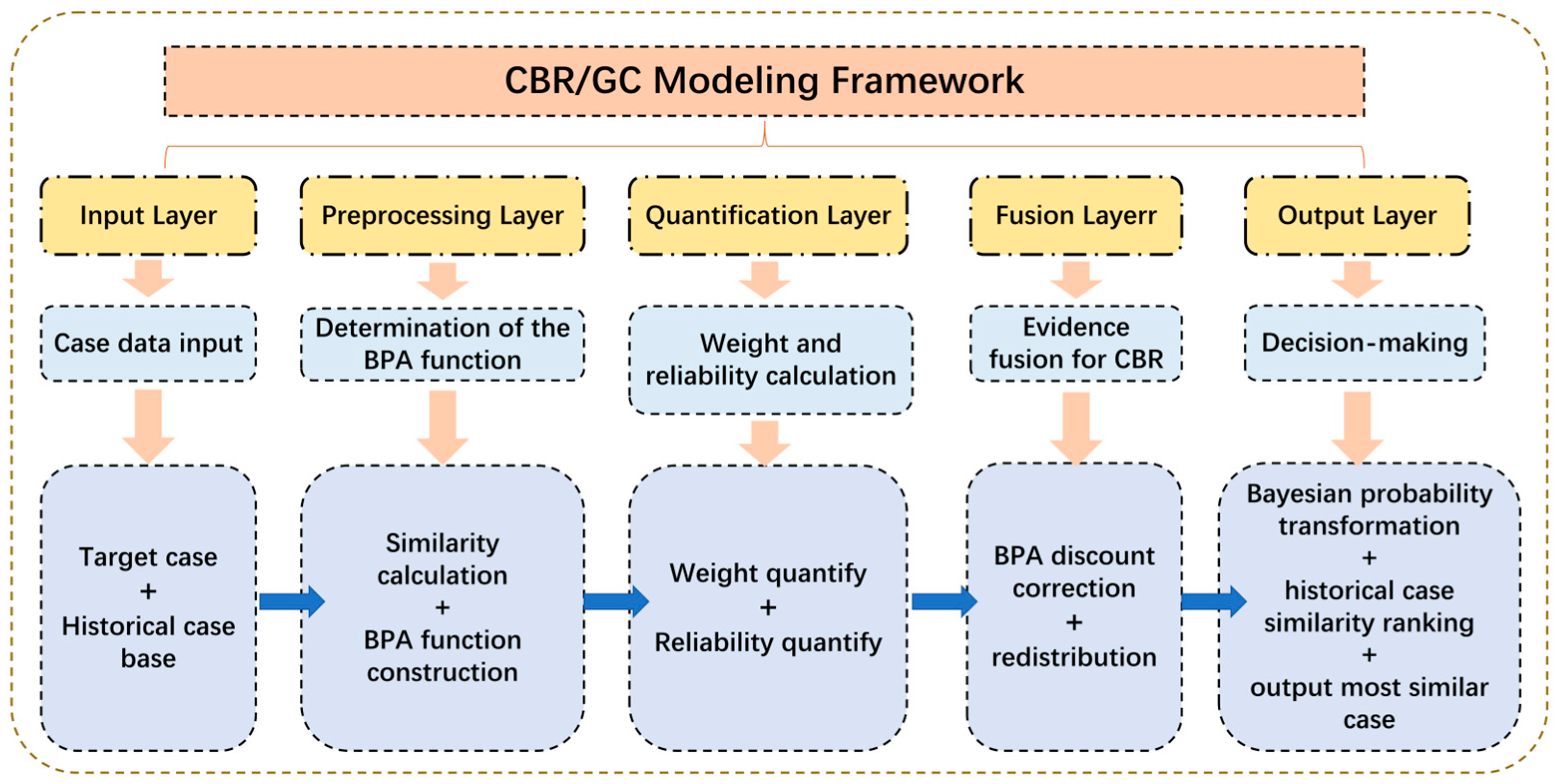
Implementing CBR/GC requires five steps: build a historical case base (frame of discernment) for the target case, calculate similarity by attribute type, convert to BPA function, determine weight and reliability, and fuse evidence via the GC rule for decisions. These steps constitute the complete CBR/GC decision-making procedure proposed in this study, as illustrated in Figure 3.

Step 1: Build a frame of discernment and case base.

Based on the problem scenario of the target case, historical cases with a similar decision-making background are selected to form a case base $C=\{c_l|l=1,2,\cdots ,L\}$, which is the frame of discernment Θ.

Step 2: Calculate the local similarity between the target case and historical cases.

For interval-type attributes, the comprehensive distance combining the center point distance and length difference is calculated using Equation (14) to obtain a similarity value $s_i^l$ in the specified range $[0,1]$. For PLTS-type attributes, the probability set structure is first adjusted according to Definition 2, followed by the calculation of similarity using Equation (15).

Step 3: Build the similarity matrix and determine the BPA function.

Construct a similarity matrix based on the local similarity calculation results. Arrange the similarities under each attribute into a matrix, grouping historical cases with identical similarity into the same grade category ${\theta }_i^n$($n=1,2,\cdots ,N_i$). Normalize the BPA values for all grade categories according to Equation (16) to obtain the final BPA function $b_i({\theta }_i^n)$, $n=1,2,\cdots ,N_i$.

Step 4: Quantify weights and reliability.

Weight calculation employs Deng entropy. For each $f_i$, Deng entropy is computed as $B_i=-{\displaystyle {\sum }_{{\theta }_i^n\subseteq \Theta }{b}_i({\theta }_i^n)·{\log }_2(b_i({\theta }_i^n)/(2^{|{\theta }_i^n|}-1))}$. Normalizing this yields ${\tilde{B}}_i=B_i/{\displaystyle {\sum }_{i=1}^I{B}_i}$, with weights defined as $w_i=(1-{\tilde{B}}_i)/( J-{\displaystyle {\sum }_{i=1}^I{B}_i})$. Reliability calculation uses Jousselme distance. Compute the lateral distance $J_{i{i}^{\prime }}=\sqrt{\frac{1}{2}{\left({\overrightarrow{b}}_i-{\overrightarrow{b}}_{i^{\prime }}\right)}^{T}D\left({\overrightarrow{b}}_i-{\overrightarrow{b}}_{i^{\prime }}\right)}$ between attribute $f_i$ and other attributes, and then calculate the global lateral average distance $J_i={\displaystyle \sum _{i^{\prime }=1}^I{J}_{i{i}^{\prime }}}/I$. Reliability is thus defined as $r_i=1-J_i$.

Step 5: Perform evidence fusion and decision-making based on the GC rule.

Use Equation (23) to discount the original BPA function $b_i({\theta }_i^n)$. Then, employ Equation (24) to recursively combine the discounted BPAs $m_{{\theta }_i^n,i}$ of all attributes, yielding the final fused probability mass $m_{\theta ,e(i)}$, $\theta \subseteq \Theta ,\theta =P(\Theta )$. Reallocate the probability involving the power set $P(\Theta )$ across the corresponding propositions according to their respective BPA proportions, thereby obtaining the standardized joint confidence $p_{\theta ,e(I)}={\widehat{m}}_{\theta ,e(I)}/(1-{\widehat{m}}_{P(\Theta ),e(I)})$, $\theta \subseteq \Theta$. Subsequently, compute the Bayesian probability for each historical case using the Bayesian approximation $\overline{m}(c_l)={\displaystyle {\sum }_{\theta \subseteq \Theta ,c_l\in \theta }{p}_{\theta ,e(I)}}/{\displaystyle {\sum }_{\theta \subseteq \Theta }{p}_{\theta ,e(I)}·\left|\theta \right|}$, $l=1,2,\cdots ,L$. Finally, decisions are made according to the maximum Bayesian probability principle, i.e., the hypothesis with the highest $c_{\ast }=\arg \max \{\overline{m}(c_l)|c_l\in C\}$ is selected as the most similar case.

4. Case Simulation Application and Analysis

4.1. Case Background

Typhoons pose severe threats to coastal communities through secondary hazards such as strong winds, torrential rainfall, and storm surges, endangering human lives, property, infrastructure, and ecosystems. China’s southeastern coastal regions face frequent typhoon events, with annual landfall counts remaining relatively stable over certain periods. Many of these typhoons are of high intensity, leading to substantial direct economic losses. Therefore, developing rapid, accurate emergency response plans is essential for improving disaster prevention and mitigation capacities. In this context, historical case analysis is a critical method for formulating effective emergency strategies.

We analyze typhoon cases that made landfall in China’s southeastern coastal regions between 2014 and 2024, focusing on three dimensions: problem characteristics, response measures, and outcomes. The problem characteristics comprise natural attributes and impact parameters, including typhoon type, maximum central wind speed at landfall, wind intensity, central minimum pressure, affected area, duration, rainfall intensity, storm surge warning level, proximity to urban centers, and population density in affected areas. Response measures capture specific management actions, such as activated emergency response levels, number of people evacuated, scope of school and business closures, traffic control implementation, emergency resource allocation, and rescue team deployment. Outcomes assess the effectiveness of emergency plans using metrics such as casualties and missing persons, direct economic losses, infrastructure damage rates, response timeliness, and public satisfaction with disaster relief operations.

To establish a typhoon disaster case base, we identify eight attributes in terms of typhoon formation, development, and dissipation (

Table 2. Attribute information, data completeness, and coefficient of variation.

Indicator	Meaning	Data Type	Completeness (%)	CV
f1	Typhoon type	Ordinal type	100	0.49
f2	Minimum Central Pressure	Numeric type	100	0.03
f3	7-Level Wind Circle Radius	Interval type	98.75	0.39
f4	10-Level Wind Circle Radius	Interval type	83.75	0.52
f5	Maximum Wind Speed	Interval type	100	0.40
f6	Wind Intensity	Interval type	100	0.24
f7	Distance from City	Interval type	80	1.24
f8	Population density of landing city	Numeric type	75	0.68

). The case base contains 80 historical typhoon cases, with

Table 3. Selected Typhoon Disaster Cases.

Case Number	Typhoon Number	f1	f2	f3	f4	f5	f6	f7	f8
1	1407	Tropical Storm	990	200		23	8–9	270–320
2	1409	Super Typhoon	910				17
3	1410	Super Typhoon	955	260–350	100–120	42	14–17
4	1415	Typhoon	960	320–480	120–140	40	13
5	1416	Severe Tropical Storm	985	200–300		28	10–11
6	1508	Super Typhoon	955	200–300	80–100	42	14–15	0–50	610
7	1510	Severe Tropical Storm	985	100–150	30–50	25	10–11	0–30	2050
8	1513	Typhoon	975	150–200	50–70	35	12–13	50–100	1100
9	1521	Super Typhoon	960	250–350	100–120	40	13–14	0–60	780
…	…	…	…	…	…	…	…	…	…
80	2421	Super Typhoon	945	380–480	180–200	60	16–17

Note: The ellipsis (…) indicates that some intermediate rows are omitted due to space limitations.

showing selected examples to demonstrate its structure. All data of the case base can be found in

Table A1. Typhoon Case Database 2014–2024.

ID	Typhoon Number	Name	Types of Typhoons	Minimum Central Pressure (hPa)	7-Level Wind Circle Radius (km)	10-Level Wind Circle Radius (km)	Maximum Wind Speed (m/s)	Wind Force Intensity (Level)	Distance from the Landing City (km)	Population Density of the Landing City (Persons/km2)	Number of Affected People (10,000 Person)	Number of Deaths (Person)	Number of Missing People (Person)	Number of People in Emergency Evacuation (10,000 Person)	Number of Collapsed Houses (Room)	Affected Area (10,000 Hectare)	Direct Economic Loss (10,000 Yuan)
1	1407	Hagibis	Tropical Storm	990	200		23	8–9	270–320
2	1409	Rammasun	Super Typhoon	910		80–80	60	17			577.3	27	5	67.4	10,900	59.2	993,000
3	1410	Matmo	Severe Typhoon	955	260–350	100–120	42	14–17			254.3	13		28.9	2600	19.02	337,000
4	1415	Kalmaegi	Typhoon	960	320–480	120–140	40	13
5	1416	Fung-wong	Severe Tropical Storm	985	200–300	50–60	28	10–11			125.4			29.3	70	3.95	95,000
6	1508	Soudelor	Severe Typhoon	955	200–300	80–100	42	14–15	0–50	610	1363	26	5	116	43,000	178	2,742,000
7	1510	Linfa	Severe Tropical Storm	985	100–150	30–50	25	10–11	0–30	2050	145	6	0	12	3200	12	315,000
8	1513	Koppu	Typhoon	975	150–200	50–70	35	12–13	50–100	1100	32	2	0	4.5	1800	8.5	86,000
9	1521	Dujuan	Severe Typhoon	960	250–350	100–120	40	13–14	0–60	780	910	10	1	82	28,000	125	1,853,000
10	1522	Mujigae	Super Typhoon	935	300–400	120–150	50	16–17	0–40	1450	1616	26	0	184	175,000	208	4,297,000
11	1601	Nepartak	Super Typhoon	900	200–350	80–150	52	16–17	0–50	3200	475	10	1	18.7	14,000	11	1,099,000
12	1603	Mirinae	Typhoon	970	100–200	40–80	35	12–13	50–100	1100	127	0	0	3.2	2300	3.8	185,000
13	1604	Nida	Severe Typhoon	945	150–300	60–120	42	14–15	0–30	6700	359	0	0	26.5	6400	7.5	789,000
14	1608	Dianmu	Severe Tropical Storm	988	80–150	20–50	25	10–11	30–80	850	103	1	0	2.1	860	2.2	123,000
15	1614	Meranti	Super Typhoon	900	250–400	100–200	52	16–17	0–20	3300	1452	28	0	184	179,000	25.5	2,904,000
16	1617	Megi	Super Typhoon	925	200–300	80–150	50	16–17	0–60	2800	855	13	0	64.9	97,000	18.2	1,773,000
17	1621	Sarika	Severe Typhoon	935	150–250	70–130	45	15–16	0–40	1500	231	1	0	18.2	12,000	4.6	428,000
18	1622	Haima	Super Typhoon	930	200–350	80–150	45	15–16	0–50	2100	453	2	0	30.2	23,000	10.8	1,935,000
19	1702	Merbok	Severe Tropical Storm	984	105–200		23	9–10		>500	>120,000	0	0				26,000
20	1707	Roke	Tropical Storm	998	50–180	120–120	18	8–9		>1000
21	1709	Nesat	Tropical Storm	955	120–250	40–40	33	12–13		800
22	1710	Haitang	Tropical Storm	985	100–150	80–120	23	9–10		800
23	1713	Hato	Super Typhoon	950	240–280	70–80	48	15–16	75	>1500		24			4000		2,891,000
24	1714	Pakhar	Severe Tropical Storm	980	150–180		28	10–12		>800
25	1716	Mawar	Tropical Storm	998	220–330	130–200	25	10–11		>800
26	1720	Khanun	Severe Typhoon	995	150–350	60–80	35	14–15		800
27	1804	Ewiniar	Tropical Storm	992	100–200	20–50	20	8–9	50–150	2500–3500	376	2	0	18	1500	27	82,000
28	1806	Kaemi	Tropical Storm	996	80–150		18	8	100–250	1500–2500	12	0	0	0.5	200	8	3500
29	1808	Maria	Super Typhoon	925	300–400	100–150	52	16	0–50	3000–4000	244.6	1	0	18.9	4500	35	114,700
30	1809	Son-Tinh	Severe Tropical Storm	988	150–250	40–70	25	10	0–40	1800–2800	30	0	0	4.2	600	15	12,000
31	1810	Ampil	Severe Tropical Storm	985	200–300	50–80	28	10	0–30	2500–3500	392	0	0	27.2	3000	46	205,000
32	1812	Jongdari	Tropical Storm	990	100–180	30–50	22	9	50–120	1800–2800	45	0	0	3.5	800	12	18,000
33	1814	Yagi	Typhoon	970	250–350	80–120	35	12	0–40	2200–3200	203	1	0	15.2	2800	29	65,000
34	1816	Rumbia	Severe Tropical Storm	980	200–300	60–100	30	11	0–20	2800–3800	795	18	1	48	13,000	87	319,000
35	1818	Mangkhut	Super Typhoon	905	400–550	150–200	65	17	0–60	3500–4500	1454	4	0	306	12,000	190	520,000
36	1822	Yutu	Super Typhoon	915	300–400	100–150	55	16	100–200	2000–3000	23	0	0	5.8	500	6	28,000
37	1823	Usagi	Tropical Storm	995	80–130		18	8	150–250	1200–2200	8	0	0	0.2
38	1905	Danas	Tropical Storm	998	150–300	150–150	18	8–9	200–300	610	14.6	0	0	1.2	50	1.2	8500
39	1907	Wipha	Severe Tropical Storm	985	200–400	50–100	25	10–11	50–100	1200	32	0	0	2.5	120	2.8	15,600
40	1910	Krosa	Tropical Storm	995	100–200	50–100	17	8–9	150–250		12	0	0	0.8	30	0.9	6200
41	1911	Bailu	Severe Tropical Storm	988	180–350	60–120	28	10–11	0	780	45.6	1	0	3.2	180	4.2	23,800
42	1914	Kajiki	Tropical Storm	1000	50–150	80–130	15	7	100–200	580	8.5	0	0	0.5	10	0.6	3500
43	1917	Sanba	Typhoon	970	250–450	80–150	35	12–13	50–100	1100	21	0	0	1.5	80	1.8	12,500
44	1919	Hagibis	Super Typhoon	910	400–600	150–300	55	≥17	500–800
45	1921	Bolaven	Severe Typhoon	950	200–350	100–180	42	14–15	800–1000
46	1924	Nakri	Tropical Storm	996	220–260	55–55	18	8–9	300–400		5	0	0	0.3	5	0.4	2100
47	1926	Kalmaegi	Tropical Storm	998	100–200	60–100	17	8–9	200–300		3.5	0	0	0.2	3	0.25	1500
48	1927	Fung-wong	Severe Tropical Storm	985	150–300	50–100	25	10–11	100–200	1050	18	0	0	1	60	1.5	9800
49	2002	Nuri	Tropical Storm	995	120–200		20	8	0	2276	26.2	0	0	1.59	12	1.42	6500
50	2003	Sinlaku	Tropical Storm	990	100–150		18	8	0	559	15.7	0	0	0.87	8	0.98	3200
51	2004	Hagupit	Severe Tropical Storm	970	200–350	50–80	35	12	0	1265	49.2	1	0	3.16	102	3.75	108,000
52	2006	Mekkhala	Typhoon	980	100–180	30–50	33	12	0	676	10.2	0	0	0.63	25	0.86	4100
53	2008	Bavi	Severe Typhoon	950	200–300	80–120	45	14	200–300	719	38.5	0	0	2.89	32	2.98	85,000
54	2017	Saudel	Typhoon	975	150–220	40–60	35	12	50–100	586	8.7	0	0	0.42	10	0.53	2800
55	2104	Koguma	Tropical Storm	992	80–150		18	8–9				0	0		0		0
56	2105	Champi	Severe Tropical Storm	985	100–200		25	10–11				0	0		0		0
57	2106	In-Fa	Typhoon	965	200–300	60–100	38	13–14	0	650–800	1479	1	0	32.2995	4175	10.702	8,752,000
58	2107	Cempaka	Typhoon	970	120–180	40–60	33	12–13	0	400	26.4	0	0	1.5743	12	0.112	52,800
59	2109	Lupit	Severe Tropical Storm	980	100–200		25	10–11	0	600	144.6	1	0	3.2156	1089	1.56	358,000
60	2117	Lionrock	Tropical Storm	990	100–180	100–200	18	8–9	0	300	24.6	0	0	1.825	35	0.285	21,000
61	2118	Kompasu	Typhoon	975	150–250	50–80	35	12–13	0	280	106.4	0	0	2.8976	65	0.685	47,000
62	2203	Chaba	Typhoon	965	200–350	80–120	35	12	0–50	620	37.2	1	0	6.1	890	45.6	402,000
63	2207	Mulan	Tropical Storm	990	100–200		20	8	0–30	410	6.5	0	0	0.85	120	8.9	38,000
64	2209	Ma-on	Typhoon	975	150–300	50–100	30	11	0–40	590	21	0	0	3.2	560	28	185,000
65	2212	Muifa	Severe Typhoon	950	300–500	100–200	42	14	0–60	1200	47	1	0	12	1200	63	325,000
66	2222	Nalgae	Severe Tropical Storm	980	150–250		25	10	0–35	380	8.2	0	0	1.1	180	12	52,000
67	2304	Talim	Severe Typhoon	950	200–350	80–150	42	14–15	0	560	27.2	1	0	1.86	320	18.5	52,000
68	2305	Doksuri	Super Typhoon	925	300–450	120–200	52	16–17	0	1700	145	14	4	18	1200	270	3,270,000
69	2309	Saola	Severe Typhoon	945	250–400	100–180	45	15–16	0	2400	37.5	2	0	3.2	580	32	1,850,000
70	2311	Haikui	Typhoon	965	180–300	60–120	35	12–13	0	650	48	6	0	5.2	450	42	860,000
71	2314	Koinu	Severe Typhoon	955	220–380	90–160	40	14–15	0	380	12	0	0	1.5	180	9.8	35,000
72	2316	Yamaneko	Typhoon	970	150–250	50–100	33	12	100–2000	600	8.5	0	0	0.8	120	8.5	12,000
73	2402	Maliksi	Tropical Storm	998	100–260		18	8	0			0	0
74	2403	Gaemi	Super Typhoon	925	250–380	100–150	58	17	0	722	90	89	52	33.5
75	2404	Prapiroon	Severe Tropical Storm	985	60–120	30–30	28	10	0		1029.5	80	9	84.4	29,000		723,000
76	2411	Yagi	Super Typhoon	905	180–300	30–80	68	17
77	2413	Bebinca	Severe Typhoon	955	100–300	60–60	42	14	0			0	0		6000		143,000
78	2414	Prasan	Tropical Storm	995	150–200	80–120	20	8	0			0	0
79	2418	Santol	Tropical Storm	982	200–250	50–100	28	10
80	2421	Kong-rey	Super Typhoon	945	380–480	180–200	60	16–17

in Appendix A. At the theoretical level, drawing on the “hazard-exposure-vulnerability” framework in disaster risk theory, attributes f₁–f₆ characterise the typhoon’s own hazard intensity and impact range, while f₇ and f₈ reflect the exposure and social vulnerability of the affected area, which are directly linked to emergency response levels and resource allocation needs. These attributes also satisfy the basic requirements of CBR in terms of discriminability and data availability. At the empirical level, based on the analysis of 80 historical typhoon cases, the average data completeness rate of the eight attributes is 92.2%, indicating good data availability. The coefficient of variation (CV) analysis (see Table 2) shows that, except for f_2, which has a narrow physical range and thus a CV of 0.03, the CVs of the remaining attributes range from 0.24 to 1.24, with f₇ reaching 1.24, demonstrating that all attributes possess sufficient discriminative power among cases.

We select Super Typhoon Ragasa (No. 2518, 2025) as the case study—a storm characterized by high intensity, direct landfall impact, and severe secondary disasters. As a landmark event in China’s natural disaster emergency response system in 2025, the scientific validity and operational effectiveness of its emergency management offer valuable insights. This case is particularly well suited for similarity matching against historical case databases (2014–2024) and comparative analysis of emergency plans in the CBR framework, thereby validating the accuracy and practical applicability of the proposed method.

4.2. CBR/GC Decision-Making Process

For emergency decision-making in typhoon disaster scenarios, CBR/GC demonstrates the reasoning process by matching the target case (Ragasa) with the historical case database.

Step 1: Calculate local similarity between the target case and historical cases.

Different similarity calculation methods are applied based on the attribute characteristics of typhoon cases. For interval-type attributes (e.g., “7-level wind circle radius,” “10-level wind circle radius,” “maximum wind speed,” “wind force intensity,” “distance from the city”), the similarity between the target case and historical cases is calculated using Equation (14). Ordinal-type attributes (e.g., “typhoon type”) are first converted into PLTS. Then, the probability set structure is adjusted according to Definition 2, followed by similarity calculation using Equation (15).

Table 4. Partial results of local similarity.

Number	f1	f2	f3	f4	f5	f6	f7	f8
1	0.2000	0.9293	0.4444	0.0000	0.3966	0.4412	0.0000	0.0000
2	1.0000	0.9891	0.0000	0.3529	0.9667	1.0000	0.0000	0.0000
3	0.8000	0.9634	0.6719	0.6000	0.7241	0.7353	0.0000	0.0000
4	0.6000	0.9583	0.5556	0.7333	0.6897	0.7647	0.0000	0.0000
5	0.4000	0.9340	0.4688	0.2188	0.4828	0.5588	0.0000	0.0000
…	…	…	…	…	…	…	…	…
80	1.0000	0.9735	0.6667	0.8824	0.9667	0.9118	0.0000	0.0000

Note: The ellipsis (…) indicates that some intermediate rows are omitted due to space limitations.

shows the partial results of the calculated local similarity.

Step 2: Build the similarity matrix and determine the BPA function.

First, the similarity values between the target case and historical cases under each attribute are compiled into a similarity matrix. Then, for every attribute, the historical cases are ranked in descending order of similarity. Cases with identical similarity values are grouped into grade categories, and the BPA for each category is calculated using Equation (16).

Table 5. Partial BPA Results.

Attribute Grade Category	f1
${\theta }_1^1$	0.0667
${\theta }_1^2$	0.1333
${\theta }_1^3$	0.2000
${\theta }_1^4$	0.2667
${\theta }_1^5$	0.3333

summarizes the results.

Step 3: Quantify weights and reliability.

First, calculate Deng’s entropy for each attribute using Equation (17). Then, normalize Deng’s entropy values for all attributes to satisfy Equation (18). Finally, compute the evidence weights using Equation (19).

Next, calculate reliability. First, compute the lateral distance between an attribute and other attributes using Equation (20). Then, calculate the global lateral average distance using Equation (21) to reflect the overall consistency of attributes. Finally, compute lateral reliability using Equation (22), converting distance into a reliability metric. The closer the reliability is to 1, the higher the consistency of that attribute with others.

Table 6. Weights and Reliability.

Attribute	f1	f2	f3	f4	f5	f6	f7	f8
Weight	0.1082	0.1295	0.1315	0.1326	0.1297	0.1281	0.1071	0.1334
Reliability	0.6156	0.7322	0.7324	0.7271	0.7240	0.7188	0.3590	0.7333

shows the results of the weight and reliability calculations.

Step 4: Perform evidence fusion and decision-making based on the GC rule.

After calculating weights and reliability, all evidence is integrated using the GC rule. First, the original BPA function of each evidence source undergoes discount correction through Equation (23), incorporating both its weight and reliability parameters. Subsequently, applying the GC rule (Equation (24)), the BPAs from all evidence sources are progressively combined to obtain the fused probability distribution. The resulting probability mass in the power set is then proportionally redistributed to corresponding propositions based on their BPA ratios, producing a normalized joint confidence distribution through Equation (28). Finally, the Bayesian probability for each proposition (historical case) in the frame of discernment is computed using Equation (13), and all of the cases are ranked in descending order. The proposition (case) with the highest probability value is identified as the most similar match to the target case. The final decision is subsequently derived by referencing the solution strategy and outcome characteristics of this optimal historical case.

In typhoon disaster emergency decision-making, the historical cases in the repository are ranked by Bayesian probability in descending order, as shown in

Table 7. Selected Bayesian Probabilities from Historical Case Database.

Number	Typhoon Number	Name	Bayesian Probability
74	2403	Gaemi	0.01323
68	2305	Doksuri	0.01318
71	2314	Koinu	0.01310
69	2309	Saola	0.01308
67	2304	Talim	0.01306
77	2413	Bebinca	0.01294
60	2117	Kujira	0.01293
61	2118	Kompasu	0.01290
58	2107	Cempaka	0.01290
50	2003	Sinlaku	0.01286
…	…	…	…
56	2105	Champi	0.01220

Note: The ellipsis (…) indicates that some intermediate rows are omitted due to space limitations.

. Typhoon 2403 Gaemi attains the highest probability, indicating that it is the most similar historical case to the target case Ragasa (2025). Its emergency response strategies—including activated emergency response level, number of evacuees and relocated individuals, and volume of allocated supplies—can be referenced to formulate more effective, scientific emergency plans.

By following the procedure outlined above, our proposed CBR/GC method fully leverages weight and reliability information to integrate multidimensional evidence. This approach enhances the accuracy and reliability of CBR outcomes, providing robust decision support for complex scenarios such as typhoon disaster management.

4.3. Simulation Comparison and Analysis of Other Methods

4.3.1. Other Methods

The CBR/GC constructed in this paper is compared with four mainstream case-based reasoning methods: the Average Operator (AO), the Weighted Average Operator (WAO), the K-Nearest Neighbors Operator (K-NNO), and the Truncation Operator (TO). The main difference among these methods lies in their approach to calculating the global similarity. It should be noted that in the comparative experiments, for handling missing attribute values, the proposed method adopts the BPA construction method based on similarity-based classification aggregation described in Section 3.2 (i.e., no direct imputation). In contrast, the other four methods employ two conventional missing data handling strategies: one is to remove case samples containing missing values, and the other is to use mean imputation to fill in the missing values, ensuring a fair comparison.

(1) Average Operator (AO). This method first computes the local similarity between the target case and each historical case under each problem attribute, denoted as $s_i^l(i=1,2,\cdots ,I,l=1,2,\cdots ,L)$. Then, the arithmetic mean of the local similarities of all attributes is taken as the global similarity, with the calculation formula given by $s^l={\displaystyle {\sum }_{i=1}^I{s}_i^l}/I$. Finally, the historical case most similar to the target case is selected based on the global similarity. This method does not consider differences in the importance of different attributes for decision-making, treating all attribute weights equally.

(2) Weighted Average Operator (WAO). This method also first calculates the local similarity $s_i^l(i=1,2,\cdots ,I,l=1,2,\cdots ,L)$, and then adopts the entropy weight method to objectively determine the weight of each attribute. The basic idea of the entropy weight method is as follows: if the similarity values of an attribute vary greatly among different historical cases, the attribute has stronger discriminative power and should be assigned a larger weight; otherwise, it should be assigned a smaller weight. Specifically, first, the proportion of the l-th historical case under the i-th attribute, $p_i^l=s_i^l/{\displaystyle {\sum }_{l=1}^L{s}_i^l}$, is calculated. Then, the entropy value of the attribute, $e_i=-{\displaystyle {\sum }_{l=1}^L{p}_i^l\ln p_i^l}/\ln L$, is computed, followed by the calculation of the coefficient of difference, $g_i=1-e_i$. Finally, the weights are obtained by normalizing the coefficients of difference, $w_i=g_i/{\displaystyle {\sum }_{i=1}^I{g}_i}$. After obtaining the weights, the weighted sum of the local similarities of each attribute is taken as the global similarity, i.e., $S^l={\displaystyle {\sum }_{i=1}^I{w}_i{s}_i^l}$, and the most similar historical case is selected accordingly [25]. This method accounts for differences in the importance of different attributes, reflecting the idea of objective weighting.

(3) K-Nearest Neighbors Operator (K-NNO). First, the global similarity between the target case and all historical cases is calculated using AO. Then, the top K historical cases with the highest global similarity are selected from the case base. The “solution type” or “case category” that appears most frequently among these K nearest neighbors is taken as the matching reference for the target case. This method introduces a nearest neighbor voting mechanism, which can effectively reduce the interference of individual abnormal cases on the retrieval results and improve the robustness of the decision-making process [31]. In this study, based on the AO calculation results, the K-NNO method selects the three historical cases closest to the target case for K-nearest neighbor classification.

(4) Truncation Operator (TO). This method optimizes the similarity aggregation result by “removing extreme values.” First, the local similarities between the target case and historical cases under each attribute are calculated. Then, the maximum and minimum local similarities are removed (to avoid interference from extreme values). The arithmetic mean of the local similarities of the remaining attributes is taken as the global similarity.

The above four methods were applied to retrieve the most similar cases from a historical case base consisting of the target case Ragasa (for typhoon disaster emergency decision-making) and 80 typhoon cases from 2014 to 2024. For each method, the two conventional missing data handling strategies were adopted: first, case deletion, i.e., deleting any historical case with missing values in any attribute, retaining only cases with complete attributes for calculation, and second, mean imputation, i.e., for each missing value, filling it with the arithmetic mean of that attribute over all non-missing cases, so that all cases have complete attribute values. Based on this, the global similarity between each historical case and the target case was calculated. The retrieval results are summarized in

Table 8. Retrieval results of other methods under different missing data handling strategies.

Method	Missing Data Handling	Effective Sample Size	Rank	Typhoon Number	Typhoon Name	Global Similarity
AO	Case deletion	46	1	2314	Koinu	0.7390
	Mean imputation	80	1	2305	Doksuri	0.7694
WAO	Case deletion	46	1	2314	Koinu	0.8572
	Mean imputation	80	1	2314	Koinu	0.7775
K-NNO	Case deletion	46	1	2314	Koinu	0.7390
			2	2305	Doksuri	0.7108
			3	2304	Talim	0.6952
	Mean imputation	80	1	2305	Doksuri	0.7694
			2	2314	Koinu	0.7390
			3	2403	Gaemi	0.7311
TO	Case deletion	46	1	2314	Koinu	0.7575
	Mean imputation	80	1	1522	Mujigae	0.7441

.

From Table 8, several observations can be made. When the case deletion strategy was adopted, all four benchmark methods selected the severe typhoon Koinu, whose intensity (955 hPa, 40 m/s) is significantly weaker than that of the target typhoon Ragasa. After switching to mean imputation, AO and K-NNO selected Doksuri, TO selected Mujigae, while WAO still retained Koinu. This indicates that the missing data handling approach significantly affects the retrieval results of traditional methods, exposing their lack of robustness to missing data. For K-NNO, under case deletion, the top three were Koinu, Doksuri, and Talim, each receiving one vote, so Koinu (with the highest similarity) was selected; under mean imputation, the top three became Doksuri, Koinu, and Gaemi, again with no majority, so Doksuri was selected. Thus, the decision result of K-NNO is influenced by both the missing data handling method and the choice of K, exhibiting a lack of consistency.

In contrast to the four benchmark methods, the proposed CBR/GC method does not rely on any form of missing value imputation or case deletion; its retrieval results are unaffected by the missing data handling strategy, demonstrating better robustness. This method directly uses all 80 historical cases for evidential reasoning, and the most similar case retrieved is Typhoon Gaemi (number 2403).

4.3.2. Matching Accuracy Comparison

To evaluate the matching accuracy of the different retrieval results, key attributes of the target typhoon Ragasa and the typhoons selected by each method are compared, as shown in

Table 9. Key attribute comparison between the target typhoon and the typhoons retrieved by different methods.

Methods	Missing Data Handling	The Typhoon Number	Name	Type	Minimum Central Pressure (hPa)	7-Level Wind Circle Radius (km)	10-Level Wind Circle Radius (km)	Maximum Wind Speed (m/s)	Wind Force Intensity (Level)	Distance from the Landing City (km)	Population Density of the Landing City (Persons/km2)
Target case	-	2518	Ragasa	Super Typhoon	920	340–380	160–180	58	17	0	327
AO/WAO/K-NNO/TO	Deletion	2314	Koinu	Severe Typhoon	955	220–380	90–160	40	14–15	0	380
AO/K-NNO	Mean imputation	2305	Doksuri	Super Typhoon	925	300–450	120–200	52	16–17	0	1700
TO	Mean imputation	1522	Mujigae	Super Typhoon	935	300–400	120–150	50	16–17	0–40	1450
CBR/GC	No imputation	2403	Gaemi	Super Typhoon	925	250–380	100–150	58	17	0	722

.

From Table 9, it can be seen that the target typhoon Ragasa is an extremely intense super typhoon. The typhoons selected by the benchmark methods have obvious shortcomings. Koinu is only a severe typhoon with a pressure of 955 hPa and wind speed of 40 m/s, significantly weaker than Ragasa; its lower bound of the 10-level wind circle is only 90 km, much smaller than Ragasa’s 160 km, so using its emergency plan would severely underestimate the risk. Doksuri, although a super typhoon with pressure 925 hPa and wind speed 52 m/s close to those of Ragasa, has a lower bound of the 7-level wind circle of 300 km, slightly smaller than Ragasa’s 340 km, and its population density is as high as 1700 persons/km²; directly applying its plan could lead to over-response. Mujigae has slightly lower intensity (935 hPa, 50 m/s) and a landing distance of 0–40 km, differing from Ragasa’s direct landfall.

In contrast, Gaemi selected by the CBR/GC method is highly consistent with Ragasa in terms of core disaster-inducing indicators. Its pressure is 925 hPa, maximum wind speed 58 m/s, and wind force level 17, compared to Ragasa’s 920 hPa, 58 m/s, and level 17; the pressure difference is only 5 hPa, and wind speed and wind force level are identical. Gaemi’s 7-level wind circle radius is 250–380 km; although the lower bound is 90 km lower than Ragasa’s 340 km, the upper bound of 380 km fully covers Ragasa’s 380 km. Its 10-level wind circle radius of 100–150 km is slightly smaller than Ragasa’s 160–180 km. The landing distance is also 0 km, indicating a direct landfall. The population density of 722 persons/km² is higher than Ragasa’s 327 persons/km² but much lower than Doksur’s 1700 persons/km², falling within a reasonable reference range.

To quantify the matching accuracy of each retrieved case, the relative errors of key attributes of each typhoon with respect to Ragasa are calculated, and the results are presented in

Table 10. Comparison of key attribute deviations.

Key Attribute	Deviation Rate (%)
	Koinu	Doksuri	Mujigae	Gaemi
Minimum central pressure	0.0380	0.0054	0.0163	0.0054
7-Level Wind Circle Radius	0.1667	0.0417	0.0278	0.1250
10-Level Wind Circle Radius	0.2647	0.0588	0.2059	0.2647
Maximum wind speed	0.3103	0.1034	0.1379	0.0000
Wind force intensity	0.1471	0.0294	0.0294	0.0000
Mean relative error	18.5%	4.8%	8.3%	7.9%

.

From Table 10, it can be seen that the mean relative error of the case Gaemi matched by the CBR/GC method is 7.9%, which is lower than those of Mujigae (8.3%) and Koinu (18.5%) but slightly higher than that of Doksuri (4.8%). It is important to emphasize that minimizing the mean relative error is not the sole optimization objective of the CBR/GC method. This method quantifies attribute weights and reliabilities using Deng entropy and Jousselme distance, respectively, and performs evidential discounting and fusion under the GC rule. The case with the highest Bayesian probability is the optimal solution that integrates the quality of decision information, rather than simply the result of minimizing numerical errors. Specifically, although Doksuri has a slightly lower mean error, its population density (1700 persons/km²) is much higher than that of Ragasa (327 persons/km²), and its lower bound of the 7-level wind circle (300 km) is insufficient compared to Ragasa’s 340 km. Under the dual discounting of weight and reliability, its comprehensive evidential support is lower than that of Gaemi. In contrast, Gaemi achieves zero deviation in maximum wind speed and wind force level, a pressure deviation of only 0.5%, and an identical landfall type. The high matching degree of these key disaster-causing factors gives it higher confidence in the evidence fusion process.

Further analysis of attribute reliabilities (see Table 6) reveals that traditional methods do not account for differences in reliability when aggregating similarities. For example, the reliability of attribute f₇ is only 0.3590, the lowest among all attributes, indicating that this attribute is highly inconsistent across different cases. However, in WAO, f₇ is assigned a weight of 0.5828 due to its high coefficient of variation, which may allow unreliable information to interfere with the decision. In contrast, the CBR/GC method, through the discounting mechanism of the GC rule, automatically reduces the influence of low-reliability attributes, thereby avoiding such bias. Another example is attribute f₂ (minimum pressure) and f₅ (maximum wind speed), both of which have high weights and high reliabilities; they receive higher confidence in the evidence fusion of CBR/GC, which is the intrinsic reason why Gaemi (zero deviation in wind speed and wind force, extremely small pressure deviation) ranks first overall.

4.3.3. Decision Rationality Comparison

The core of decision rationality lies in whether the emergency response plan of the matched case can provide an effective reference for the target case. The target typhoon Ragasa is a direct landfall typhoon with extremely high intensity (920 hPa, 58 m/s, level 17), a 7-level wind circle of 340–380 km, a 10-level wind circle of 160–180 km, and a relatively low population density. Therefore, an ideal matching typhoon should be highly similar to Ragasa in terms of disaster intensity (pressure, wind speed, wind circle radius), maintain consistency in landfall type, and allow for scaling of response measures based on exposure indicators such as population density.

First, consider the three typhoons selected by the benchmark methods. Koinu is only a severe typhoon (955 hPa, 40 m/s), significantly weaker than Ragasa; its lower bound of the 10-level wind circle is only 90 km, much smaller than Ragasa’s 160 km; referencing its emergency plan would severely underestimate the destructive power. Doksuri, though a super typhoon with pressure and wind speed relatively close to those of Ragasa, has a lower bound of the 7-level wind circle of 300 km, slightly smaller than Ragasa’s 340 km, and an extremely high population density of 1700 persons/km²; directly applying the response measures from such a high-density area could lead to over-mobilization and waste of resources. Mujigae has slightly lower intensity (935 hPa, 50 m/s) and a landing distance of 0–40 km; although this interval includes 0 km, it is not a completely direct landfall, and its emergency experience may include buffer measures suitable for non-direct landfalls, which are not fully applicable to Ragasa.

In contrast, Gaemi, selected by the CBR/GC method, is the most balanced and highly consistent match with Ragasa in terms of core disaster-indicating indicators. First, the intensity parameters are nearly identical. Gaemi has a pressure of 925 hPa, a maximum wind speed of 58 m/s, and a wind force level 17, compared to Ragasa’s 920 hPa, 58 m/s, and level 17; the wind speed and wind force level achieve zero deviation, and the pressure deviation is only 0.5%. Second, the wind circle structure is reasonable. Gaemi’s 7-level wind circle radius is 250–380 km; although the lower bound is 90 km lower than Ragasa’s, the upper bound of 380 km fully covers Ragasa’s 380 km, meaning the upper limit of the strong wind influence range is consistent. Its 10-level wind circle radius of 100–150 km is slightly smaller than Ragasa’s 160–180 km, but in a direct landfall scenario, the 10-level wind circle affects only a narrow area near the eyewall; this can be compensated by appropriately expanding the warning zone around the predicted landfall point, without altering the decision framework. Third, the landfall type is completely identical. Gaemi has a landing distance of 0 km, also a direct landfall, so its experience in personnel evacuation timing, traffic control scope, pre-positioning of emergency forces, etc., can be directly transferred.

Moreover, Gaemi’s population density is 722 persons/km², approximately 2.2 times that of Ragasa (327 persons/km²). This difference is favorable for emergency decision-making: Gaemi successfully underwent emergency response under a higher population density, and its successful experiences (e.g., evacuation organization, material allocation, multi-agency coordination) can be appropriately scaled down for Ragasa’s lower population density, forming a “downward reference.” This is more reliable and safer than an “upward reference” from low density to high density.

From the perspective of decision logic, traditional methods rely only on simple aggregation of similarity values and do not account for the reliability of decision information or the dynamic differences in attribute importance. The CBR/GC method’s ability to accurately identify Gaemi is due to two core innovations. First, the method quantifies attribute uncertainty using Deng entropy to determine weights, evaluates attribute consistency using Jousselme distance to characterize reliability, and performs evidential discounting and fusion under the GC rule, thereby automatically assigning higher weights to key disaster-causing factors such as pressure, wind speed, and the 7-level wind circle, while reducing the interference of low-reliability attributes. It is this mechanism that gives Gaemi, with zero deviation in maximum wind speed and wind force level, the highest comprehensive support. Second, the method does not require imputation of missing values or deletion of cases; it directly constructs basic probability assignments using all cases, avoiding information loss and artificial bias, and maintains a 100% sample utilization rate. Therefore, the decision-making process of the CBR/GC method better meets the practical needs of typhoon disaster emergency decision-making, and it significantly outperforms traditional methods in matching accuracy, decision rationality, and data adaptability.

4.4. Results and Discussion

Based on the reasoning process and fusion results of the CBR/GC method, we identify Gaemi as the historical case most similar to the target case Ragasa. To evaluate the effectiveness of CBR/GC for typhoon disaster emergency decision-making, we examine the results from three perspectives: similarity alignment accuracy, the effect of weight–reliability integration, and practical decision-making value.

4.4.1. Similarity Matching Accuracy

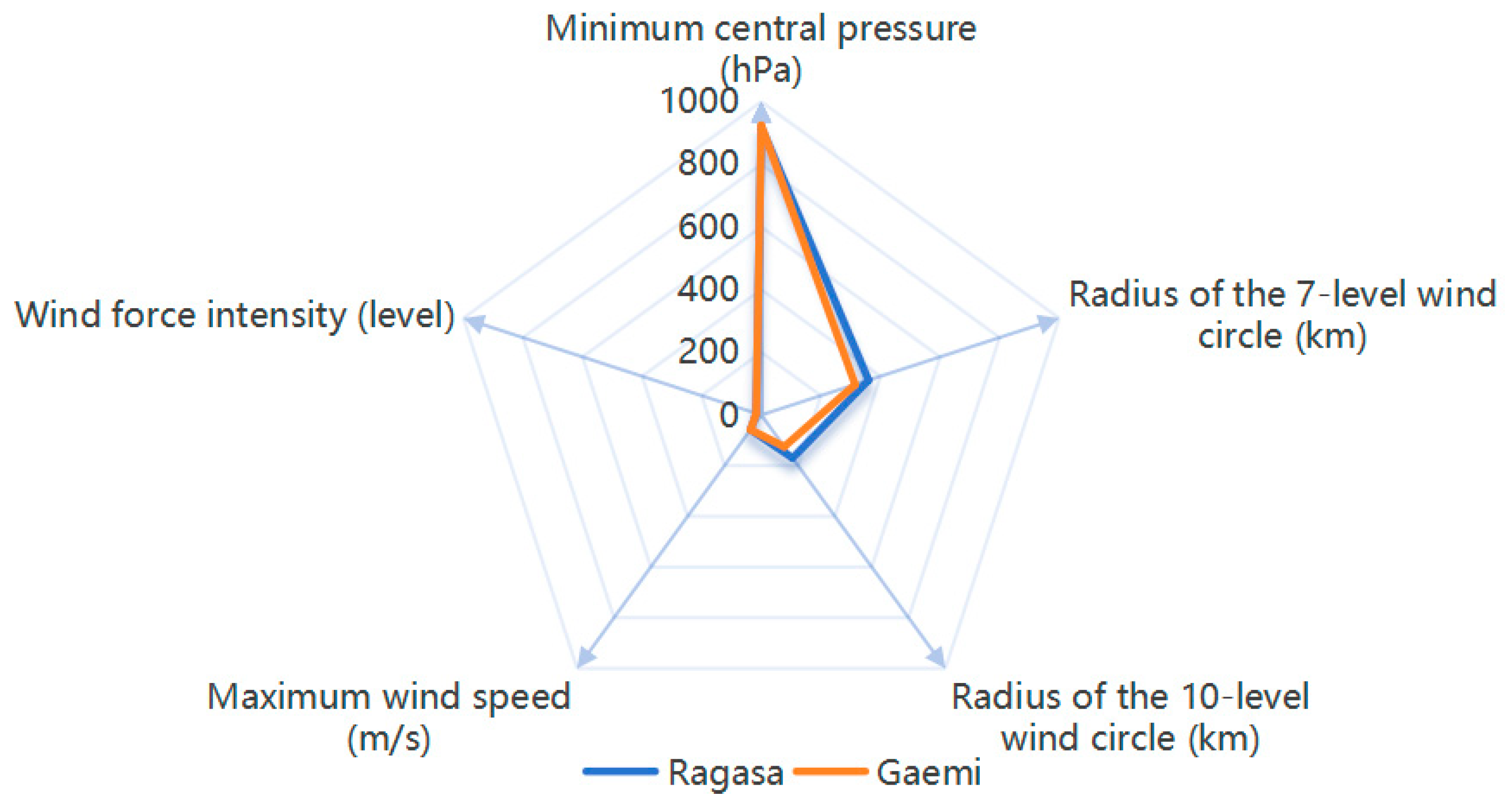
The CBR/GC method identifies Typhoon Gaemi (2403) as the optimal match, with a Bayesian probability of 0.01323, significantly higher than that of the second-ranked candidate (Doksuri, 2305) at 0.01318. This indicates a clear differentiation capability. To validate the rationality of the matching results, we compare key attributes between Typhoon Ragasa and Gaemi, addressing a core requirement of typhoon emergency decision-making—contingency plans must simultaneously account for both intensity parameters and impact scope. Given that these attributes have different physical units (e.g., pressure, distance, wind speed), absolute errors are not directly comparable. We therefore adopt the average relative error as the primary accuracy metric, as it normalizes these differences and provides an intuitive percentage deviation. Through matching deviation rate analysis (

Table 11. Comparison of deviations in key attributes between target and matched Cases.

Key Attribute	Target Case	CBR/GC Matched Case	Deviation Rate
Minimum central pressure (hPa)	920	925	0.5%
7-Level Wind Circle Radius (km)	340–380	250–380	12.5%
10-Level Wind Circle Radius (km)	160–180	100–150	26.5%
Maximum wind speed (m/s)	58	58	0
Wind force intensity (level)	17	17	0
Average relative error	-	-	7.9%

and Figure 4), the average relative error between Typhoon Ragasa and Gaemi across critical attributes is 7.9%. Notably, the maximum wind speed and wind force intensity deviations are 0% (both 58 m/s and level 17), and the minimum central pressure deviation is only 0.5% (925 hPa vs. 920 hPa), confirming the excellent alignment in core intensity parameters.

In terms of similarity matching accuracy, the two typhoons exhibit strong correlation across core attributes. Their meteorological structures demonstrate notable consistency: the minimum central pressure differs by only 5 hPa (0.5%), while maximum wind speed and wind force are perfectly identical (58 m/s, level 17). Regarding wind field structure, Gaemi’s 7-level wind circle radius (250–380 km) covers the entire upper bound of Ragasa’s range (340–380 km), indicating that the overall affected area is well matched. Although the 10-level wind circle of Gaemi (100–150 km) is smaller than that of Ragasa (160–180 km), this discrepancy can be mitigated by expanding the precautionary buffer zone, as discussed in the practical decision-making section. Furthermore, both typhoons made direct landfall, a critical factor for emergency response planning.

It is worth noting that the average relative error of Gaemi (7.9%) is slightly higher than that of Doksuri (4.8%), as shown in the comparative study (Section 4.3). This does not indicate a flaw in the CBR/GC method; rather, it reflects that the method optimizes a composite objective that incorporates evidence weight and reliability, not merely numerical error minimization. Doksuri possesses a lower numerical error but has a much higher population density (1700 persons/km² vs. Ragasa’s 327), and its 7-level wind circle lower bound (300 km) is below Ragasa’s lower bound (340 km). Through the GC rule’s discounting mechanism, attributes with lower reliability (e.g., distance to city) and mismatched exposure characteristics are penalized, making Gaemi the top choice in the fused belief distribution.

4.4.2. Effect of Weighting and Reliability

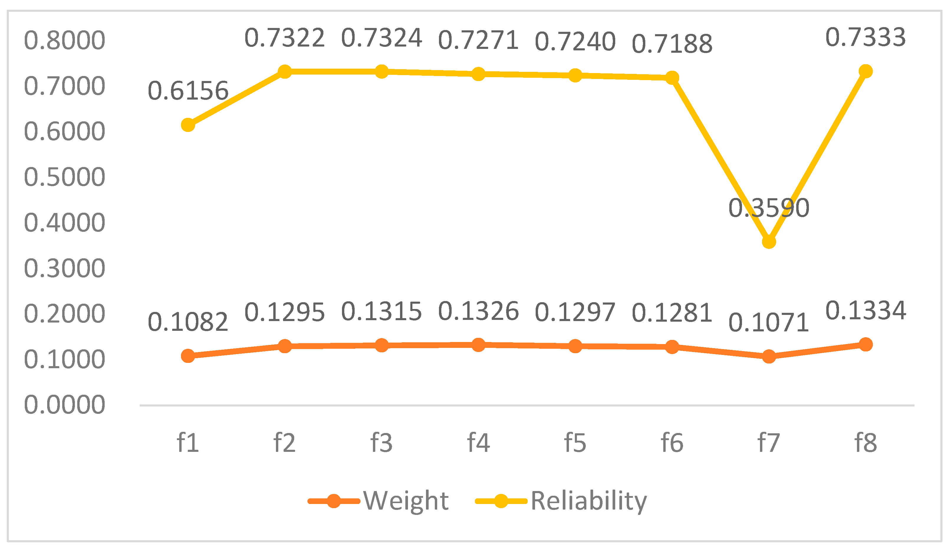
Regarding weight and reliability, the weights assigned to attribute characteristics range from 0.1071 to 0.1334 (Figure 5), indicating a relatively balanced distribution. Wind circle–related attributes (f₃ and f₄) carry more weight, underscoring their critical role in determining typhoon impact areas for emergency decision-making. Population density (f₈) has the highest weight (0.1334), while distance from city (f₇) receives the lowest (0.1071), reflecting their relative discriminative power. Reliability parameters demonstrate notable variation, with “distance to urban areas” (f₇) showing the lowest reliability—reflecting its inconsistent alignment with other attributes across cases. Conversely, the “population density of landing cities” (f₈) achieves the highest reliability, indicating its stable performance throughout the case repository. These differential weight and reliability assignments capture both the importance and consistency of each attribute, thereby enhancing the differentiation capacity of the decision model.

The combined effect of weight and reliability manifests in the evidence discounting process. Attributes characterized by both high weight and strong reliability receive enhanced confidence during fusion, whereas those with substantial weight but moderate reliability undergo systematic discounting prior to integration. This strategy maintains their influence while reducing the effect of uncertainty. For example, the “distance to urban areas” attribute, despite showing exceptional similarity in specific instances, is subject to appropriate moderation during fusion owing to its generally low reliability. This dual mechanism prevents any single, less reliable attribute from exerting disproportionate influence on the final decision, thereby improving the robustness of the results.

4.4.3. Practical Decision-Making Value

The essence of rational decision-making lies in whether the solution derived from a matched case can provide actionable guidance for the target case. In terms of disaster impact and response requirements, Typhoon Ragasa’s direct landfall and high intensity demand prioritized personnel evacuation and infrastructure protection. In this regard, Typhoon Gaemi’s emergency response characteristics offer a highly relevant reference value. As shown in

Table 12. Comparison of Emergency Scenarios in Matched Cases.

Key Attributes	Target Case (Ragasa)	CBR/GC Matched Case (Gaemi)
Distance from Landing City (km)	0	0
Wind Intensity (Beaufort Scale)	17	17
Maximum Wind Speed (m/s)	58	58
7-Level Wind Circle Radius (km)	340–380	250–380
10-Level Wind Circle Radius (km)	160–180	100–150

, Gaemi also made direct landfall, and its intensity parameters are almost identical. The 7-level wind circle covers the same upper bound as Ragasa’s, and the 10-level wind circle is smaller but manageable through expanded buffer zones. Consequently, Gaemi’s response strategy—including emergency level activation, evacuation scale, transportation control, and resource pre-positioning—provides a solid reference for formulating Ragasa’s emergency plan.

From a decision-making perspective, traditional methods rely on the simplistic aggregation of similarity metrics without accounting for dynamic variations in information reliability and attribute importance; this results in limited adaptability to complex scenarios. By contrast, the CBR/GC method quantifies attribute contributions through weighting—assigning higher confidence to critical factors such as minimum central pressure and wind circle radius—while filtering evidence through reliability assessment. By integrating these dimensions using the GC rule, this method generates belief distributions that better align with the practical requirements of typhoon disaster emergency decision-making, ultimately producing more actionable and applicable outcomes.

In terms of practical decision-making value, the Gaemi case offers a highly comparable reference, with its emergency response plan providing critical guidance for Ragasa. As a high-intensity typhoon, Gaemi established benchmarks in terms of emergency response level, resource-allocation scale, and evacuation zoning, providing a foundation for Ragasa’s preparedness. Successful evacuation route planning, shelter site arrangements, and operational protocols from Gaemi can be directly adapted for Ragasa, particularly for large-scale evacuations. By analyzing Gaemi’s resource consumption patterns and allocation experience, more accurate predictions can be made regarding the types and quantities of supplies required for Ragasa, thereby optimizing stockpiling and distribution strategies. Furthermore, the specific challenges encountered during Gaemi’s response can deliver critical risk alerts for Ragasa’s emergency management, enabling the proactive deployment of targeted preventive measures.

From the matching results, several actionable insights can be distilled for real-world emergency management. First, the radius of the 7-level wind circle is more critical than that of the 10-level wind circle. The complete coverage of the upper bound of the 7-level wind circle determines the overall evacuation and resource allocation scale, whereas deviations in the 10-level wind circle can be compensated by enlarging the precautionary buffer zone. Second, emergency experience from moderately high-density areas can be safely scaled down to low-density settings. The successful adaptation of Gaemi’s response to Ragasa’s lower-density scenario demonstrates that response levels and evacuation scales can be proportionally adjusted according to population density while keeping the core decision framework transferable. Third, the low reliability of the distance-to-city attribute suggests that the exact landfall point is inherently uncertain; emergency planning should therefore incorporate a buffer interval rather than relying on a precise zero-distance assumption. These insights go beyond mere result reporting and provide operational guidance for typhoon emergency decision-making.

5. Conclusions

Traditional CBR methods often overlook the weight and reliability of decision information and struggle with attribute heterogeneity and missing data. This undermines the accuracy and robustness of decision-making in complex scenarios such as emergency management.

We propose the CBR/GC method to address these limitations. Our approach first designs differentiated similarity calculation strategies for heterogeneous attributes, including interval-type and PLTS data. Historical cases with identical similarity values are classified and aggregated to construct a BPA function, thereby addressing missing data without direct imputation. Attribute weights are determined by quantifying uncertainty through Deng entropy, while reliability is characterized by measuring consistency using Jousselme distance. Discounted BPA is then recursively fused via the GC rule, with final decisions derived through Bayesian probability transformation. A case study of typhoon disaster emergency decision-making demonstrates the method’s effectiveness and practicality. Our three main contributions are as follows:

(1)

Innovative handling of missing data. Our method avoids direct imputation by constructing BPA through similarity-based classification. Missing attributes are treated as uncertain information and embedded in the evidence framework, preserving data uncertainty while reducing traditional imputation bias. This enhances adaptability to incomplete datasets.

(2)

Unified framework for heterogeneous attributes. Our unified framework transforms numerical, intervallic, symbolic, probabilistic, and ordinal attributes into interval-type and PLTS representations. Differentiated similarity strategies are designed for each type, enabling consistent cross-attribute comparison and effective fusion within a single reasoning structure.

(3)

Dual characterization of weight and reliability. Weights and reliability are quantified via Deng entropy and Jousselme distance, respectively. Their synergistic integration in the GC rule enables multidimensional evidence quality control, which improves the robustness and credibility of final decisions.

Nevertheless, the proposed method has certain limitations. First, like most data-driven approaches, its performance is influenced by the quality and completeness of historical case data. However, unlike traditional CBR methods, our approach can indirectly handle missing data through similarity-based BPA construction, thereby avoiding imputation bias. Nonetheless, in scenarios with extremely sparse or highly noisy data, the accuracy may still be affected. Second, the computational complexity of evidence fusion increases with the number of attributes and cases, which may limit real-time application in time-sensitive scenarios (e.g., emergency response). Third, the current case study focuses on a single typhoon event. Although this case effectively demonstrates the feasibility of the method, further validation through multi-case or sensitivity analyses is needed.

Beyond the above technical limitations, several implementation challenges should be considered. Regarding data availability, the method requires a well-structured historical case base, which in practice is often incomplete or inconsistent, necessitating substantial preprocessing and expert input. Regarding real-time computation, the recursive fusion under the GC rule incurs high computational overhead when the number of cases or attributes is large; for time-critical scenarios (e.g., emergency evacuation), dimensionality reduction or parallel computing may be needed. Regarding operational adoption, decision-makers require training to interpret Bayesian probabilities, and the method assumes historical cases are independent and identically structured; violation of this assumption (e.g., non-stationary case distributions) may affect performance.

These limitations and implementation considerations do not undermine the value of the proposed CBR/GC method; rather, they point to promising directions for future research, including (1) developing adaptive mechanisms for dynamic case-base updating; (2) optimizing the computational efficiency of the fusion process; (3) extending validation with multiple test cases across different application domains and geographic regions; and (4) designing user-friendly decision support interfaces that translate evidence fusion outputs into actionable recommendations for practitioners.