A Multi-Head Attention Soft Random Forest for Interpretable Patient No-Show Prediction

Abstract

Unattended scheduled appointments (“patient no-shows” henceforth) adversely affect healthcare providers and patients’ health, disrupting the continuity of care, operational efficiency, and allocation of medical resources. Therefore, accurate predictive modeling is needed to reduce the impact of patient no-shows. Although machine learning methods, such as logistic regression, random forests, and decision trees, are widely used to predict patient no-shows, they often rely on hard decision splits and static feature importance, limiting adaptability to complex patient behaviors. To address this limitation, we propose a hybrid multi-head attention soft random forest (MHASRF) model that integrates attention mechanisms into a random forest using probabilistic soft splitting. It assigns attention weights across the trees, enabling attention on specific patient behaviors. The MHASRF model exhibited an accuracy of 88.24%, specificity of 91.21%, precision of 81.60%, recall of 82.01%, F₁-score of 81.81%, and area under the receiver operating characteristic curve of 94.07%, demonstrating high and balanced performance across metrics. It could also identify key predictors of patient no-shows at two feature-importance levels (tree and attention mechanism), providing deeper insights into patient no-shows. Thus, the proposed MHASRF model is a robust, adaptable, and interpretable method for predicting patient no-shows that can help healthcare providers optimize resources.

1. Introduction

Patients who do not attend scheduled appointments (“patient no-shows” henceforth) pose a major problem in healthcare systems, impacting both patients and healthcare providers. For healthcare providers, patient no-shows lead to increased operational costs, decreased operational efficiency, and reduced clinic revenue. For patients, missing appointments disrupts continuity of care and wastes valuable appointment slots, thereby increasing waiting times for others and contributing to patient dissatisfaction [1,2,3]. Given these multifaceted consequences, accurately predicting patient no-shows has become essential for optimizing healthcare service delivery.

To address the challenge of reducing patient no-shows, hospitals and clinics have implemented various operational strategies, including automated appointment reminder systems, overbooking policies, and predictive modeling techniques to anticipate whether a patient will attend a scheduled appointment [4,5]. In this context, predictive modeling has emerged as a particularly promising tool because of its ability to handle complex patterns in patient behavior.

Due to the inherently uncertain nature of patient no-show behavior, prior research has often employed machine learning methods, such as logistic regression (LR), naïve Bayes (NB), and random forest (RF) [6,7,8,9]. Other techniques, such as adaptive boosting (AdaBoost), extreme gradient boosting (XGBoost), gradient boosting (GB), bagging, and support vector machine (SVM), have also been used to predict patient no-shows [10,11,12]. Complementing these methods, neural network-based models, such as deep neural networks (DNNs), artificial neural networks (ANNs), and multilayer perceptrons (MLPs), have been used to better capture high-dimensional, nonlinear relationships in the data [13,14].

Attention mechanisms have improved predictive modeling by enabling machine learning models to focus on relevant information [15], which is particularly useful for structured healthcare data, where complex feature interactions can affect prediction outcomes. Traditional machine learning models such as LR, decision trees (DTs), and RFs are widely used for structured healthcare data because they are relatively interpretable and robust [6]. However, they may be limited in capturing complex feature interactions and instance-specific patterns. In contrast, deep learning models can learn intricate patterns, but their black-box nature limits their adoption in sensitive domains such as healthcare [16]. Therefore, integrating attention mechanisms into a tree-based framework offers a promising balance between predictive capability, interpretability, and robustness [17].

Recent studies have begun integrating attention mechanisms into RF models for healthcare applications. For example, self-attention-enhanced RF models have been proposed for breast cancer classification [18], and attention-augmented RF models have demonstrated promising performance in various conditions, including diabetes mellitus [19]. Despite these developments, their application to real-world clinical decision-making problems, particularly for predicting patient no-shows, remains relatively unexplored.

To address this gap, we aimed to develop a hybrid model that integrates an attention mechanism into a soft RF (SRF) model. Specifically, we extend traditional RFs by incorporating soft DTs (SDTs) [20], replacing hard splits with probabilistic soft splits. This enhancement allows for smoother decision boundaries and better handling of uncertainty in no-show behavior.

In addition, because no-show behavior varies across patients and appointment contexts, an adaptive mechanism is needed to produce patient-appointment-specific predictions while preserving interpretability. Therefore, we introduce a trainable attention mechanism and a tree reliability parameter to enhance the SRF model. This enhancement enables instance-specific attention weighting across trees, combining the interpretability and robustness of an SRF with the adaptive feature-focusing capabilities of an attention mechanism. Our proposed model can adjust tree contributions based on the characteristics of each appointment, making it well-suited to structured healthcare prediction tasks.

Moreover, traditional RF models derive feature importance solely from tree splits [21]. Therefore, we employ a dual-level feature importance analysis at both the tree and attention-mechanism levels to provide a more comprehensive understanding of the factors driving patient no-show behavior. This analysis can offer deeper insights into model behavior and may support more informed scheduling decisions in healthcare settings.

By integrating attention mechanisms with an SRF, our proposed model aims to balance predictive performance, interpretability, and robustness in predicting patient no-shows. We introduce a novel approach to attention-based modeling within probabilistic RF frameworks, offering new insights into improving the understanding of patient no-show behavior, appointment scheduling, and operational efficiency in healthcare systems.

The remainder of this paper is organized as follows. Section 2 reviews the related literature. Section 3 describes the theoretical foundation, the proposed framework, the model architecture, data preprocessing, and the experimental setup. Section 4 presents the results and their interpretations. Section 5 presents the limitations and future directions. Finally, Section 6 concludes by highlighting the key findings and discussing future work.

2. Literature Review

The problem of patient no-shows has been a focus of healthcare research since the early 1980s [22]. Research on patient no-shows has evolved from LR [23] to more advanced statistical and probabilistic methods. As computational advances emerged, recent research has sought to leverage machine learning and related methods to address patient no-shows. Such research aims to optimize medical services by reducing waiting times and minimizing resource wastage, ultimately improving the efficiency of healthcare providers. The growing list of hospital patients demands improved services through increasing use of “smart” digital facilities.

To address patient no-shows, research has employed various methodologies, ranging from probabilistic methods, such as NB and Bayesian networks, to machine learning methods, such as RFs, ANNs, and k-nearest neighbor (k-NN) [8,24]. In one study [8], DTs achieved greater accuracy than NB (94.5% vs. 85.0%), and both methods outperformed LR. In addition, DTs have been applied to 33,329 dermatology and 21,050 pneumonology samples to develop a system to reduce patient no-shows to hospital appointments [10].

Some studies have solely employed regression-based methods, rather than machine learning methods. For instance, one study [25] developed 24 unique LR-based models to predict veterans’ attendance at healthcare appointments, identifying key predictors, such as prior attendance history and patient age, as critical determinants of no-show inquiries. Similarly, another study [6] developed an LR-based model to improve patient management in a bariatric clinic and identified additional predictors of patient no-shows, including the distance from home to the clinic and the number of prior appointments. Notably, their model was less impacted by highly personal details, such as age group and gender. A central focus of these studies was the selected predictors of patient no-shows. The most notable common features identified in these studies were patient demographics, past no-show history, booking times, and appointment schedules.

Additionally, studies have employed probabilistic approaches to develop effective strategies for overbooking scenarios. For instance, one study [26] integrated the elastic net (EN) variable selection method with the probabilistic Bayesian belief network (BBN). An EN was used for feature selection, and a BBN was used for prediction. Unlike the NB method [27], BBNs enable investigation of interrelationships among predictors of patient no-shows. Building on prior research, one study [28] aimed to address patient no-shows by combining a probabilistic model (LR) with an advanced machine learning model (GB). Among the methods considered, GB achieved the highest accuracy (78%) and F₁-score (0.76).

More recently, as the influence of artificial intelligence (AI) has grown, several studies have employed AI techniques to address patient no-shows. While some earlier studies focused solely on LR-based methods, more recent studies [11,29] compared techniques such as AdaBoost, SVMs, balanced RFs, and DTs separately or in combination against LR-based methods. For instance, one study [22] compared the Hoeffding and JRip algorithms for modeling and classification of patient appointments, which yielded similar accuracies of 77.13% and 76.44%, respectively. Similarly, another study [12] found that DTs outperformed AdaBoost in both precision (0.89 vs. 0.87) and recall (0.86 vs. 0.83). However, they found that DTs were highly susceptible to computational complexity limitations.

While most prior studies have focused primarily on predicting patient no-shows in individual clinics, one [8] addressed this issue within the Saudi dental healthcare system. It employed DT, RF, and MLP models to predict patient no-shows, finding that the RF model outperformed the MLP model in this specialized setting. In addition, unlike most prior studies that have focused solely on offline factors, one study [30] considered both offline and online factors to model outpatient appointments and predict patient no-shows. It employed various machine learning techniques, including bagging, k-NN, boosting, LR, and DTs, to predict patient no-shows. It concluded that the bagging model outperformed the other models in predicting patient no-shows based on online factors.

The number of patient no-shows is often lower than the number of attended appointments, leading to biased models. Several studies [11,30,31] have employed data balancing to address this issue. For instance, one study [11] employed random under-sampling boosting (RUSBoost), balanced RF, balanced bagging, and easy ensemble models, and minimized the weighted average of type I and type II errors. Another study [30] applied a synthetic minority oversampling technique (SMOTE) to a training dataset to obtain a more balanced sample. A further study [31] combined minority-class oversampling with majority-class undersampling.

Most prior research has focused on machine learning and deep learning architectures to predict patient no-show behavior. Recently, attention mechanisms have been developed to improve classification and regression algorithms by automatically aligning feature importance and weighting. First introduced for machine translation [32], attention mechanisms have become crucial components in neural networks. The foundational concept of attention can be interpreted using a regression model [33,34]. In the seminal study [32], attention was part of a recurrent neural network–based encoder–decoder to encode long input sentences. The transformer architecture [35] eliminates sequential processing and yields highly accurate results for machine translation without recurrent components. Various attention-based models have been previously reviewed [15].

RF is a robust alternative to neural networks. Recently, some studies have begun integrating attention mechanisms into RF models [18,19,36]. For instance, one study [18] combined self-attention with an RF model to classify breast cancer, while another study [19] used an attention mechanism to assign weights to DTs in an RF model. A further study [36] extended prior work [19] by applying attention and self-attention in RF models.

Despite significant progress in prior studies, none have applied the novel approach of attention mechanisms to address the problem of patient no-shows. Therefore, this study aimed to address this gap by introducing a novel hybrid multi-head attention SRF (MHASRF) model that integrates attention mechanisms into an SRF using probabilistic soft splitting. The proposed model aims to improve prediction accuracy by leveraging the strengths of both techniques, such as interpretability and robustness, while addressing the limitations of previous approaches.

3. Materials and Methods

3.1. Theoretical Framework

3.1.1. Soft Decision Tree

While DTs are fast and interpretable, they suffer from drawbacks such as overfitting and non-differentiability, making them challenging to use in gradient-based optimization. SDTs address these limitations by replacing hard splits with smooth and probabilistic decisions [20]. SDTs allow for a continuous gradient, making the model differentiable and suitable for backpropagation during training. SDTs are also trained with a classification objective and an additional regularization term to support stable learning [20]. The probabilistic decision in each inner node is defined as follows [20]:

$$p_i\left(x\right)=\sigma \left(x{w}_i+b_i\right),$$

(1)

where the filter $w_i$ and the bias $b_i$ are learnable parameters in each inner node i, x is the input to the model, and $\sigma$ is the sigmoid function.

3.1.2. Random Forest

An RF is an ensemble technique that aggregates predictions from multiple DTs to improve accuracy and robustness [21]. In this study, we incorporate SDTs into the RF framework, enabling differentiability for gradient-based optimization. This modified ensemble, referred to as SRF, preserves the robustness of traditional RFs while leveraging the flexibility of SDTs to enhance model adaptability.

3.1.3. Attention Mechanism

The attention mechanism plays a crucial role in enabling machine learning models to focus on relevant parts of the input data. It assigns weights to the input, allowing the model to assign important features selectively. This mechanism has been widely applied in deep learning, particularly in models such as transformers, which use self-attention to process input sequences. The attention mechanism consists of three components: queries, keys, and values [35].

A prior study developed an attention-based RF (ABRF) model [19], introducing an attention mechanism into a traditional RF. In the ABRF model, the attention weight α is assigned based on the instances x that fall into the same leaf node of a DT (distance); closer instances receive more attention, and distant instances get less attention. The query, key, and value are denoted by x, A_k(x), and B_k(x), respectively. Here, the input instance x is the query, A_k(x) denotes the average vector of instances that fall into the same leaf node as x in the kth SDT, and B_k(x) represents the average target value (i.e., the mean of the target label vectors y) for those instances that fall into the same leaf node as x in the kth SDT. The distance $D_k$ between the query and the key is defined as follows:

$$D_k\left(x,\tau \right)=softmax \left(-{\displaystyle \frac{{‖x-A_k\left(x\right)‖}^2}{2\tau }}\right),$$

(2)

where $\tau$ is a tuning parameter (temperature) of the softmax function. In the original ABRF model, attention weights are computed using several approaches, including a contamination model, a softmax function, and a combination of the two, via trainable parameters. An ABRF model with a softmax function is formulated as follows:

$$\alpha \left(x,A_k\left(x\right),v,z\right)=softmax\left(-{\displaystyle \frac{{‖x-A_k\left(x\right)\circ z‖}^2}{2}}{v}_k\right),$$

(3)

where $v_k$ is the vector of trainable parameters, z is the training vector of the feature weights, and $v_k$ is the training parameter, which incorporates the temperature $\tau$ in Equation (2).

However, a preliminary study found that the conventional ABRF performed poorly on our problem. Therefore, instead of directly adopting this trainable parameter, we proposed a novel trainable parameter δ to dynamically adjust the attention scores. This parameter is specifically designed to leverage the tree-wise reliability information from the SRF model. By incorporating this new trainable parameter into the distance computation, the model is expected to be more adaptive, dynamically adjusting attention weights based on both the tree reliability and the instance distance. More reliable SDTs (with lower errors) receive greater attention, while less reliable SDTs receive less attention. Additionally, we employ multi-head attention rather than single-head attention to capture diverse patterns across heads and model complex feature dependencies and interactions, which are crucial in predicting patient no-shows. The details of the new trainable parameter δ and multi-head attention are described in Section 3.2.3.

3.2. Proposed Framework

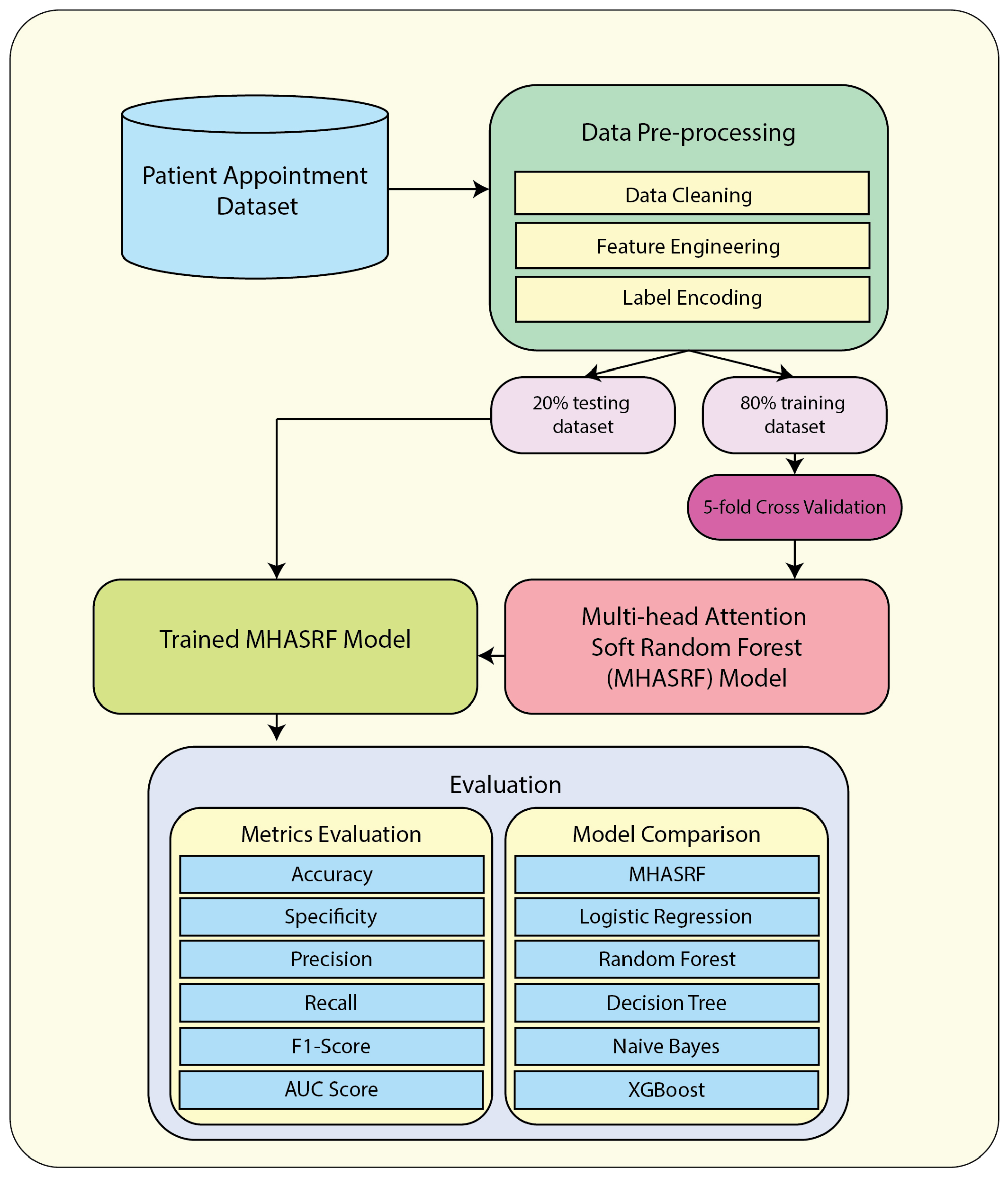
In this section, we present the proposed framework for predicting patient no-shows (Figure 1). It begins with data collection and data preprocessing, then proceeds to model architecture, and concludes with evaluation.

The overall framework begins by preprocessing the patient appointment dataset, including data cleaning, feature engineering to enrich the features, and label encoding to convert categorical variables to numerical variables. Once the data are preprocessed, they are split into training and testing sets. The processed data is fed into the predictive model and first processed using an SRF model. During the training phase of the SRF model, each SDT k generates a mean vector A_k(x) and a mean target value B_k(x) while simultaneously computing a tree error, which is used to estimate the tree reliability parameter δ_k. Next, multi-head attention is applied to each SDT, and the resulting representation is passed through an MLP to enhance the final prediction, followed by a softmax function. To ensure robustness, we used 5-fold cross-validation during model training. In the evaluation phase, we assess the MHASRF model’s performance using several metrics, including accuracy, specificity, precision, recall, and F₁-score. We compare the MHASRF model against baseline models, including LR, RF, DT, NB, and XGBoost.

3.2.1. Data Collection

This study used a dataset of de-identified appointment-related administrative records from a major healthcare provider in the Middle East. Due to confidentiality agreements, detailed information about the healthcare provider cannot be disclosed. The dataset includes appointment records from January 2018 to December 2018, totaling 157,494 appointments. We only consider appointments that patients either attended (show) or missed (no-show), excluding canceled appointments. Each appointment record captured information under the following categories:

• Patient characteristics: age, gender, and language.
• Appointment characteristics: appointment status, type of visit, reason for visit, appointment time, specific healthcare provider, and others.
• Clinic and provider: the type of clinic and the name of the physician.

3.2.2. Data Preprocessing

To extract useful and relevant information from the dataset, it is essential to preprocess the data before passing it to the model. We performed data cleaning, feature engineering, and categorical data encoding to enhance data quality and improve model performance.

• Data cleaning: Data were cleaned to reduce noise, handle missing data, and remove outliers and irrelevant features.
• Feature engineering: New features were derived from the data. For instance, the feature “Percentage of No-shows” (% no-show) was calculated for each patient based on their appointment history prior to the target appointment. Similarly, the feature “Number of Visits” was defined as the number of visits prior to the target appointment. In addition, the feature “Number of Appointments on the Same Day” was defined as the number of appointments scheduled for that day. Thus, all history-based features were constructed using only information available up to the target appointment, without using the target outcome or any future appointments.
• Encoding categorical variables: The dataset primarily contains categorical variables, such as gender, reason for the visit, month of the appointment, and type of visit. We transformed categorical variables into numerical representations using label encoding.

After cleaning and standardizing, the final dataset used for the model contained 101,532 medical appointments and 24 predictive features (

Table 1. The input features of the model.

Feature	Description	Type	Source
Patient Characteristics
Age	The patient’s age at the time of the appointment	Continuous	Raw
Language	The patient’s preferred language	Categorical	Raw
Gender	The patient’s gender	Categorical	Raw
Visit Reason	The reason for the patient’s visit	Categorical	Raw
Appointment Characteristics
Visit Type	The type of visit (e.g., procedure, consult, or new)	Categorical	Raw
Appointment Status	The current status of the appointment (i.e., no-show or show)	Categorical	Raw
Time Appointment by Time	The exact time of the appointment	Continuous	Raw
Time Appointment by Day	The day on which the appointment is scheduled	Categorical	Raw
Time Appointment by Month	The month in which the appointment is scheduled	Categorical	Raw
Week of The Month	The week number within the month in which the appointment is scheduled	Categorical	Derived
Season	The season during which the appointment is scheduled (e.g., summer or winter)	Categorical	Derived
Number of Visits	The number of visits the patient had before this appointment date/time	Continuous	Derived
%No-Show	The percentage of the patient’s prior appointments that were no-shows	Continuous	Derived
Number of Appointments on The Same Day	The number of appointments the patient had on the same day	Continuous	Derived
Clinic and Provider
Institute	The healthcare institute where the appointment is scheduled	Categorical	Raw
Center Name	The specific center within the institute where the appointment is scheduled	Categorical	Raw
Department Name	The department within the center where the appointment is scheduled (e.g., dentistry, gynecology, or urology)	Categorical	Raw
Provider Name	The name of the healthcare provider (physician) assigned to the patient	Categorical	Raw
External Factors
Temperature	The outside temperature at the time of the appointment	Continuous	Derived
Dew	The dew point (moisture level in the air) at the time of the appointment)	Continuous	Derived
Humidity	The humidity level at the time of the appointment	Continuous	Derived
Windspeed	The wind speed at the time of the appointment	Continuous	Derived
Visibility	The visibility level at the time of the appointment	Continuous	Derived
Weather Conditions	General description of the weather (e.g., raining, cloudy, or clear)	Categorical	Derived
Air Quality	The description of the air quality index (e.g., good, moderate, unhealthy, or hazardous)	Categorical	Derived

). Among these, 68,520 cases (67.49%) were “show” appointments and 33,012 cases (32.51%) were “no-show” appointments, indicating a moderate class imbalance. No additional data balancing technique was applied because the class distribution was moderately, rather than severely, imbalanced, and we aimed to preserve the original appointment distribution of the data. The dataset was split into a training set (80%) and a held-out testing set (20%).

3.2.3. Model Architecture

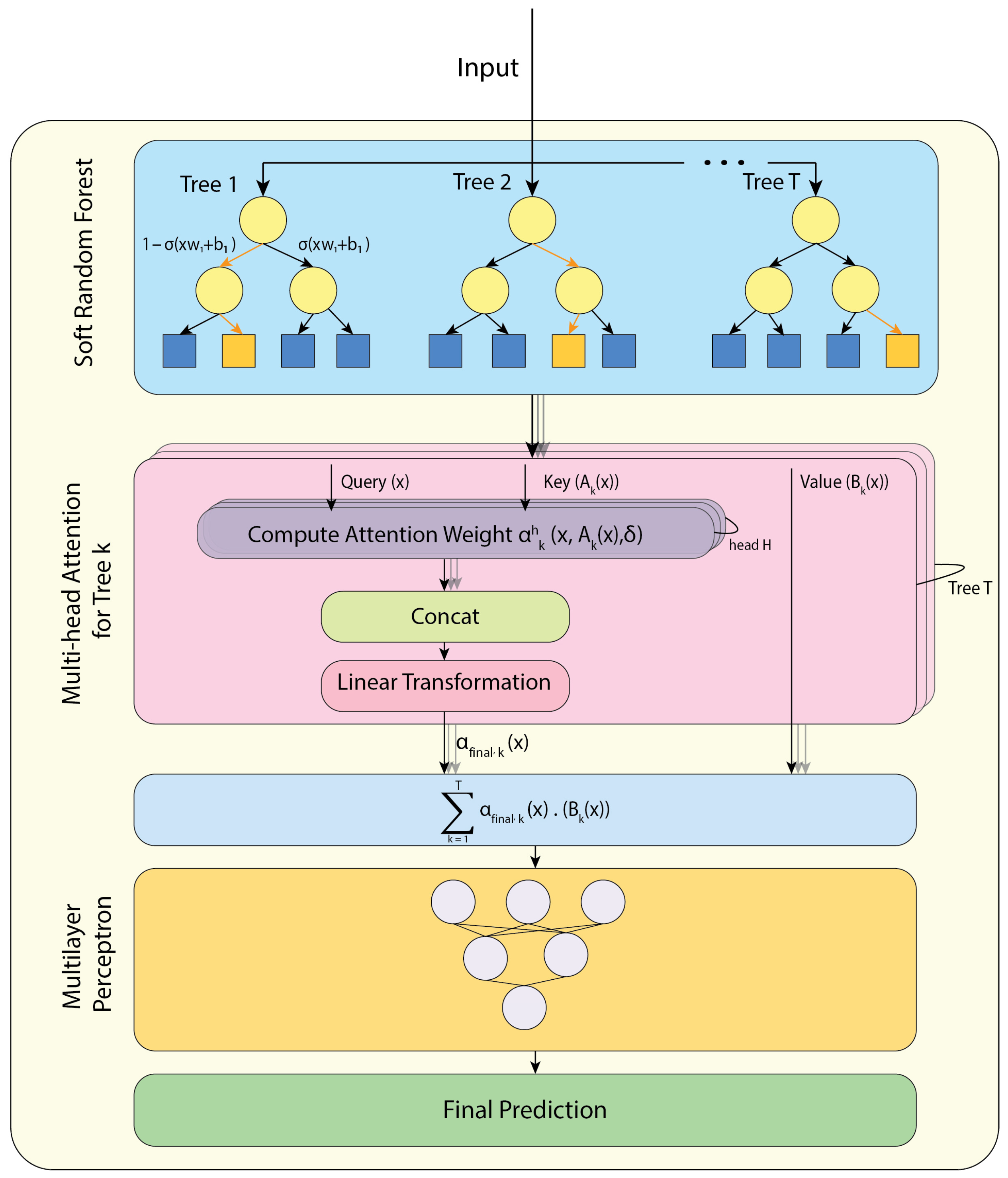
The overall architecture of the MHASRF model is illustrated in Figure 2. It begins with an input layer that receives the preprocessed feature vector $x\in {\mathbb{R}}^d$, where d represents the number of input features. In practice, the MHASRF model is implemented in two stages.

In the first stage, an SRF is constructed using SDTs. Each SDT is trained on a bootstrap sample of the training set using the cross-entropy classification loss. After the SRF is trained, each training instance is passed through every SDT to obtain its leaf assignment. Based on these leaf assignments, A_k(x), the average input factor of the training samples assigned to the same leaf as the input x in SDT k, and B_k(x), the average target vector of those samples, are computed.

The tree error C_k for each trained SDT is also estimated, which determines the tree reliability parameter δ_k. To quantify tree reliability, we define the tree error C_k as the average misclassification rate of tree k as follows:

$$C_k={\displaystyle \frac{1}{n}}{\displaystyle \sum _{s=1}^n}1\left(B_k\left(x_s\right)\ne y_s\right) ,$$

(4)

where n is the number of samples, y_s is the true value, and 1(·) is the indicator function. The tree error C_k and the tree reliability parameter δ_k are both scalars, since each represents a single value per SDT. To make δ_k(x) trainable, we introduce the trainable parameter λ, leading to the following formulation:

$${\delta }_k= {\displaystyle \frac{{\lambda }^H}{C_k}} ,$$

(5)

where H is the number of attention heads. SDTs with higher tree reliability parameter δ_k values have lower errors (higher reliability) and contribute more significantly to the final decision, while those with higher errors (lower reliability) contribute less.

In the second stage, the multi-head attention mechanism is applied, where x is the query, A_k(x) is the key, and B_k(x) is the value. To compute multi-head attention for each tree k, we define the attention weight $\alpha$ for each head as follows:

$${\alpha }_k^h\left(x, A_k\left(x\right),\delta \right)=softmax \left({\delta }_k^h- {\displaystyle \frac{{‖x-A_k\left(x\right)‖}^2}{2\tau }}\right),$$

(6)

where τ is a tuning (temperature) parameter. The attention weight ${\alpha }_k^h$ is a scalar since it represents a single weight per head. The softmax normalization is applied across SDTs for each attention head, so that the attention weights for a given head sum to 1 over all SDTs.

The attention weight ${\alpha }_k^h$ in Equation (6) combines two important components: the tree reliability parameter ${\delta }_k^h$ and the distance ${‖x-A_k\left(x\right)‖}^2$. The first term, ${\delta }_k^h$, reflects how reliable the SDT is, with higher values indicating greater reliability. This parameter is derived from the inverse of the tree error C_k, encouraging the model to place greater weight on more accurate SDTs. The second term, ${‖x-A_k\left(x\right)‖}^2$, represents the distance between instance x and the average vector of instances in the same leaf node as x, reflecting how relevant the SDT is for the input. A smaller distance indicates greater relevance.

By combining the tree reliability and distance terms, the attention weight ${\alpha }_k^h$ becomes more adaptive, enabling the model to assign greater weight to the SDTs that are more accurate and relevant to the input. This change is expected to improve overall prediction performance.

After computing the attention weights, the attention outputs across all heads are concatenated into a single vector:

$${\alpha }_{concat,k}\left(x\right)= \left[{\alpha }_k^1,{\alpha }_k^2,{\alpha }_k^3,\dots ,{\alpha }_k^H\right],$$

(7)

where ${\alpha }_{concat,k}\left(x\right) \in {\mathbb{R}}^H$ is an H-dimensional vector, and H is the total number of attention heads.

To aggregate information across multiple attention heads, we apply a linear transformation using the trainable weight matrix $W_H\in {\mathbb{R}}^{H \times H}$ that projects the concatenated attention weights for SDT k into a new space, allowing the model to learn optimal weight distributions across heads. The final attention weight for SDT k, which remains an H-dimensional vector, is defined as follows:

$${\alpha }_{final,k}\left(x\right)= W_H{\alpha }_{concat,k}\left(x\right)$$

(8)

A weighted sum of tree predictions is then computed and passed through an MLP to enhance the final prediction:

$$y_{final}=MLP\left({\displaystyle \sum _{k=1}^T}{\alpha }_{final,k}\left(x\right)B_k\left(x\right)\right)$$

(9)

In the final step, a softmax function is applied after the MLP to ensure the output is a probability distribution with all class probabilities summing to 1. The final prediction $\widehat{y}$ is a vector given as follows:

$$\widehat{y}=softmax \left(y_{final}\right)$$

(10)

After computing class probabilities using the softmax function (Equation (10)), the final class label is determined by applying a decision rule in which a threshold of 0.5 is used for the binary classification task. The overall training procedure of the MHASRF model is summarized in Algorithm 1.

Algorithm 1. Multi-head Attention Soft Random Forest Model

Input:    Dataset $\mathcal{D}=\left\{\left(x,y\right)\right\}, x \in {\mathbb{R}}^d, y \in \{0,1\}$    Number of trees T, tree depth D, number of attention heads H, number of epochs E Output:    Trained MHASRF model    Global feature importance $I_{final}\in {\mathbb{R}}^d$ 1.   Initialize forest: 2.     for k = 1 to T: 3.      SDTk ← SDT (depth = D, input dim = d, output dim = 2) 4.      add SDTk to the forest 5.   Train SDTs: 6.     for each SDTk in the forest: 7.      ${\mathcal{D}}_k$ ← bootstrap sample of $\mathcal{D}$ 8.      for epoch = 1 to E: 9.          train $SD{T}_k$ on $D_k$ using cross-entropy classification loss 10. Compute leaf statistics and tree reliability: 11.   for each SDTk: 12.       Pass training samples through SDTk to obtain leaf assignments 13.      Precompute Ak(x) and Bk(x) 14.      Ck ← average misclassification on $\mathcal{D}$ 15.      δk ← λH/Ck 16.     Multi-head attention: 17.     initialize λ1 ∈ ${\mathbb{R}}^H$ and W ∈ ${\mathbb{R}}^{H\times H}$ 18.     for batch X in $\mathcal{D}$: 19.      for each SDT k: 20.       obtain the leaf assignment of each input x in SDT $k$ 21.       retrieve the corresponding Ak(x) and Bk(x) 22.      for each tree k and head h: 23.          ${\alpha }_k^h\leftarrow softmax \left({\delta }_k^h- {\displaystyle \frac{{‖x-A_k\left(x\right)‖}^2}{2\tau }}\right)$ 24.      for each SDT k: 25.          ${\alpha }_{concat,k}\left(x\right)= \left[{\alpha }_k^1,{\alpha }_k^2,{\alpha }_k^3,\dots ,{\alpha }_k^H\right],$ 26.          ${\alpha }_{final,k}\left(x\right)\leftarrow W_{H · }{\alpha }_{concat,k}\left(x\right)$ 27.      $y_{final}\leftarrow MLP\left({\displaystyle {\sum }_{k=1}^T}{\alpha }_{final,k}\left(x\right)B_k\left(x\right)\right)$ 28.      $\widehat{y}\leftarrow softmax \left(y_{final}\right)$ 29.     Feature importance: 30.      for each feature xj: 31.      Itree(xj) ← average absolute weight across nodes and trees 32.      Iattention(xj) ← attention-weighted tree importance 33.      Ifinal (xj) ← average the Itree(xj) and Iattention(xj) 34.     Optimize parameters via cross-entropy loss and Adam

3.3. Feature Importance

Understanding which factors influence patient attendance at appointments is essential to reducing no-shows and enhancing the quality of healthcare services. By identifying key factors, hospitals and clinics can take proactive steps to reduce patient no-shows. Therefore, we compute feature importance using our proposed MHASRF model by integrating tree-level importance (I_tree) and attention-level importance (I_attention).

I_tree measures the contribution of each feature within individual SDTs by quantifying how often a feature is used in decisions at the internal nodes of the SDT at the SRF level. SDTs in the SRF allow all features to contribute to a node’s decision via learnable weights [20]. Thus, we define I_tree as the aggregation of the absolute weights across all internal nodes and SDTs. Formally, I_tree for feature $x_j$ in SDT k is evaluated as follows:

$$I_{tree,k}\left(x_j\right)={\displaystyle \frac{1}{{\mathcal{N}}_k}}{\displaystyle \sum _{n=1}^{{\mathcal{N}}_k}}\left|w_{k,n,j}\right|,$$

(11)

$$I_{tree}\left(x_j\right)={\displaystyle \frac{1}{T}}{\displaystyle \sum _k^T}{I}_{tree,k}\left(x_j\right),$$

(12)

where T is the total number of SDTs, ${\mathcal{N}}_k$ is the number of internal nodes in the kth SDT, and $w_{k,n,j}$ is the weight of feature $x_j$ at internal node n in SDT k. A larger weight indicates a stronger influence of that feature on routing decisions within the SDT.

I_attention is derived from the final attention weights ${\alpha }_{final,k}\left(x\right)$, which capture each SDT’s contribution. A feature is considered more important if it strongly contributes to the decision function of nodes within the SDTs that receive greater attention. We computed I_attention as follows:

$$I_{attention}(x_j)={\displaystyle \frac{1}{T}}{\displaystyle \sum _{k=1}^T}{\alpha }_{final,k}\left(x\right) · I_{tree,k}\left(x_j\right)$$

(13)

Both importance measures are scalar. Finally, we combine both global importance measures by averaging their contributions. I_tree and I_attention are first normalized separately, and the final feature-importance score is then obtained by averaging the two normalized components with equal weights. This step ensures that feature importance reflects both feature usage in SDTs and the learned weighting from the attention mechanism. These importance scores provide valuable insight into the key features influencing patient attendance at appointments, empowering hospitals and clinics to implement strategies that reduce patient no-shows.

3.4. Loss Function and Optimization

To optimize the MHASRF model, we used the cross-entropy loss function, which is commonly used for classification [37]. The loss function is designed to incorporate tree reliability parameters δ_k and multi-head attention. It is defined as follows:

$$\mathcal{L}=-{\displaystyle \frac{1}{n}}{\displaystyle \sum _{i=1}^n}{\displaystyle \sum _{c=1}^C}{y}_i^{c}log{\widehat{y}}_i^c,$$

(14)

where n, C, $y_i^c$, and ${\widehat{y}}_i^c$ are scalar values that represent the number of training samples, the number of classes (no-show and show), the true class label, and the predicted probability for class c, respectively. ${\widehat{y}}_i^c$ is obtained using Equation (10). The model is trained using the adaptive moment estimation (Adam) optimizer to update the network parameters.

3.5. Evaluation Metrics

Classification model performance is often evaluated using metrics such as accuracy, recall (sensitivity), specificity, precision (or positive predictive value [PPV]), negative predictive value (NPV), and F₁-score, which are computed based on a confusion matrix consisting of true positive (TP), false positive (FP), false negative (FN), and true negative (TN) values:

• TP: The model correctly predicts that the patient will be a no-show.
• FP: The model incorrectly predicts that the patient will be a no-show.
• TN: The model correctly predicts that the patient will attend the appointment.
• FN: The model incorrectly predicts that the patient will attend the appointment.

The evaluation metrics are defined as follows:

$$Accuracy= {\displaystyle \frac{TP+TN}{TP+TN+FP+FN}} ,$$

(15)

$$Recall={\displaystyle \frac{TP}{TP+FN}} ,$$

(16)

$$Specificity={\displaystyle \frac{TN}{TN+FP}},$$

(17)

$$Precision (PPV)={\displaystyle \frac{TP}{TP+FP}},$$

(18)

$$NPV={\displaystyle \frac{TN}{TN+FN}},$$

(19)

$$F_1 Score=2\times {\displaystyle \frac{Precision\times Recall}{Precision+Recall}}$$

(20)

3.6. Experimental Setup

We compared our proposed MHASRF model with DT, RF, LR, NB, and XGBoost models in terms of accuracy, specificity, precision, recall, and F₁-score. We selected these alternative model architectures for comparison because they have been commonly used as benchmarks in prior studies [6,7,8,9,27]. All experiments were conducted on a 7th-generation Core i7 CPU with a maximum speed of 2.10 GHz. The models were developed using the scikit-learn (ver. 1.6.1) and PyTorch (ver. 2.10.0) libraries in Python (ver. 3.12.13).

The dataset was initially split into training (80%) and held-out testing (20%) sets. All records from the same patient were assigned to a single subset, ensuring that no patient appeared in both training and testing sets. The same grouping strategy was applied during 5-fold cross-validation within the training set. Therefore, no patient appeared in both the training and validation folds. This procedure was used to prevent data leakage and to ensure an evaluation of unseen patients.

The MHASRF model used the following hyperparameters: number of SDTs = 100, tree depth = 3, number of attention heads = 3, and learning rate = 0.01. These hyperparameters were selected empirically by varying the main model settings during model development. The final configuration was chosen because it consistently produced strong predictive performance without introducing unnecessary computational cost or model complexity.

4. Results and Discussion

In this section, we present the experimental results obtained with the proposed MHASRF model. We evaluated its predictive performance, conducted statistical analyses, and compared its performance with that of various traditional models. We also examined the distribution of attention weights and identified the key features that significantly influence patient no-shows based on feature importance. Moreover, we conducted an ablation study to assess the contribution of model components, a stratified analysis, and a contextual comparison with previous studies.

4.1. Performance Comparison with Baseline Models

4.1.1. Performance in 5-Fold Cross-Validation

The validation results for the MHASRF and baseline models are shown in

Table 2. Predictive performance of the MHASRF and baseline models in 5-fold cross-validation.

Model	Accuracy	Specificity	Precision	Recall	F1-Score	AUC
MHASRF	88.00% ± 0.30%	90.47% ± 0.61%	80.79% ± 0.70%	82.88% ± 1.33%	81.82% ± 0.52%	93.91% ± 0.35%
DT	88.29% ± 0.21%	89.50% ± 0.35%	79.79% ± 0.36%	85.78% ± 0.66%	82.67% ± 0.33%	93.03% ± 0.18%
RF	85.35% ± 0.65%	95.41% ± 0.24%	87.18% ± 0.32%	64.53% ± 2.33%	74.14% ± 1.54%	93.14% ± 0.27%
LR	86.82% ± 0.26%	87.66% ± 0.34%	76.92% ± 0.26%	85.08% ± 0.94%	80.79% ± 0.44%	90.86% ± 0.33%
NB	83.17% ± 0.48%	81.65% ± 0.59%	69.46% ± 0.65%	86.30% ± 0.89%	76.97% ± 0.64%	86.86% ± 0.55%
XGBoost	88.77% ± 0.22%	90.57% ± 0.03%	81.35% ± 0.04%	85.02% ± 0.05%	83.14% ± 0.03%	94.43% ± 0.15%

Abbreviations: AUC, area under the receiver operating characteristic curve; DT, decision tree; LR, linear regression; MHASRF, multi-head attention soft random forest; NB, naïve Bayes; RF, random forest; XGBoost, extreme gradient boosting.

. We used 5-fold cross-validation to evaluate model performance, and the results are presented as the mean ± standard deviation across folds, reflecting the consistency of each model’s results. The MHASRF model demonstrated strong and stable performance in the 5-fold cross-validation, with an accuracy of 88.00% ± 0.30%, specificity of 90.47% ± 0.61%, precision of 80.79% ± 0.70%, recall of 82.88% ± 1.33%, F₁-score of 81.82% ± 0.52%, and area under the receiver operating characteristic (ROC) curve (AUC) of 93.91% ± 0.35%. These results indicate that the MHASRF model performs consistently across folds and maintains a balanced predictive performance across metrics.

Among the baseline models, the XGBoost model demonstrated the strongest overall performance, with the greatest accuracy (88.77% ± 0.22%), specificity (90.57% ± 0.03%), precision (81.35% ± 0.04%), recall (85.02% ± 0.05%), F₁-score (83.14% ± 0.03%), and AUC (94.43% ± 0.15%). The DT model also performed well, achieving slightly higher recall (85.78% ± 0.66%) and F₁-score (82.67% ± 0.33%) than the MHASRF model.

The RF model demonstrated the greatest specificity (95.41% ± 0.24%) and precision (87.18% ± 0.32%) but significantly lower recall (64.53% ± 2.33%), failing to detect many actual patient no-shows (TPs). The LR model demonstrated relatively balanced performance, with an F₁-score of 80.79% ± 0.44%, but its AUC (90.86% ± 0.33%) remained lower than those of the MHASRF and other tree-based baseline models. The NB model demonstrated the weakest overall performance, with the lowest accuracy, precision, F₁-score, and AUC. Overall, although several baseline models achieved slightly better predictive performance, the MHASRF model remained competitive and showed balanced performance across evaluation metrics.

4.1.2. Performance in the Held-Out Testing Set

To further evaluate the generalizability of the MHASRF model, we assessed its performance on a held-out testing set that was not used during training or cross-validation. In this analysis, the MHASRF model remained competitive with balanced overall performance (

Table 3. Comparison of predictive performance across models on held-out test data.

Model	Accuracy	Specificity	Recall	Precision	NPV	F1-Score	AUC
MHASRF	88.24%	91.21%	82.01%	81.60%	91.42%	81.81%	94.07%
DT	88.43%	89.82%	85.51%	79.98%	92.88%	82.65%	93.18%
RF	85.15%	96.36%	61.56%	88.94%	84.06%	72.76%	93.38%
LR	86.63%	87.98%	83.78%	76.82%	91.94%	80.15%	90.54%
NB	83.09%	81.87%	85.65%	69.20%	92.30%	76.55%	86.23%
XGBoost	88.82%	90.79%	84.68%	81.38%	92.57%	83.00%	94.50%

), achieving an accuracy of 88.24%, specificity of 91.21%, recall of 82.01%, precision of 81.60%, NPV of 91.42%, F₁-score of 81.81%, and AUC of 94.07%. These results confirm that the MHASRF model generalizes well to unseen cases and maintains strong discriminative performance in the held-out testing set.

Among the baseline models, the XGBoost model demonstrated the strongest overall performance, with high accuracy (88.82%), recall (84.68%), F₁-score (83.00%), AUC (94.50%), and NPV (92.57%), while also maintaining strong specificity (90.79%) and precision (81.38%). The DT model also demonstrated high accuracy (88.43%), recall (85.51%), F₁-score (82.65%), and NPV (92.88%). However, the MHASRF model demonstrated greater specificity (91.21%) and precision (81.60%) than both the DT (89.82% and 79.98%, respectively) and XGBoost (90.79% and 81.38%, respectively) models and a higher AUC than the DT model (94.07% vs. 93.18%). These findings indicate that the MHASRF model remains competitive and well-balanced, with particular strengths in specificity, precision, and class discrimination.

The RF model demonstrated high precision (88.94%) and the highest specificity (96.36%) but lower recall (61.56%) and NPV (84.06%). Thus, although the RF model was effective in reducing FPs, it missed a substantial number of TPs. The LR model demonstrated relatively balanced performance, with a recall of 83.78% and an NPV of 91.94%, but its AUC was lower than those of the MHASRF and tree-based baseline models. The NB model performed worst across most metrics, particularly PPV (69.20%), indicating inflated FPs. However, its NPV (92.30%) was relatively high, suggesting it remained more reliable at predicting TNs than at predicting TPs.

Overall, the held-out testing results indicate that the XGBoost model performed best overall across evaluation metrics, including accuracy, recall, F₁-score, AUC, and NPV. However, the MHASRF model remained competitive and well-balanced, outperforming both the XGBoost and DT models in specificity and precision and the DT model in AUC. These results suggest that the MHASRF model offers a favorable predictive profile, particularly in settings where minimizing FP predictions is important while maintaining reliable TN predictions.

In a healthcare system, failing to identify patients who are likely to miss scheduled appointments (i.e., FN) may result in resource waste, care disruptions, longer waiting times, and increased operational costs [1,2,3]. Conversely, when a patient expected to be a no-show actually attends (i.e., FP), this may lead to unnecessary interventions, overbookings, or rescheduling. Therefore, the clinical usefulness of a patient no-show prediction model should be evaluated not on a single metric alone, but on its overall balance across practically relevant performance measures, including PPV and NPV.

The PPV and NPV provide additional insight into the reliability of model predictions. The MHASRF model achieved a PPV of 81.60%, indicating that most patients predicted as no-shows were correctly classified, and an NPV of 91.42%, indicating strong reliability in identifying patients likely to attend appointments. Although the XGBoost model achieved the highest NPV among the compared models, the MHASRF model achieved a slightly higher PPV than the XGBoost model and a higher PPV than the DT, LR, and NB models. Thus, the MHASRF model may be particularly useful in clinical settings where reliable identification of likely patient no-shows is important for targeted interventions, reminder systems, and operational planning.

Overall, the MHASRF model demonstrated competitive, well-balanced performance on the held-out testing set. Although the XGBoost model achieved greater accuracy, recall, F₁-score, and AUC, the MHASRF model achieved higher specificity and precision, indicating greater strength in minimizing FP predictions. This performance profile suggests that the MHASRF model offers a favorable trade-off between identifying patients at risk of no-show (TPs) and avoiding excessive false predictions (FPs). Such a balance may be particularly valuable in real clinical settings, where overly aggressive no-show prediction may itself introduce operational inefficiencies. Thus, the held-out testing results support the MHASRF model as a clinically meaningful approach to predicting patient no-shows, particularly when balanced predictive behavior is an important consideration.

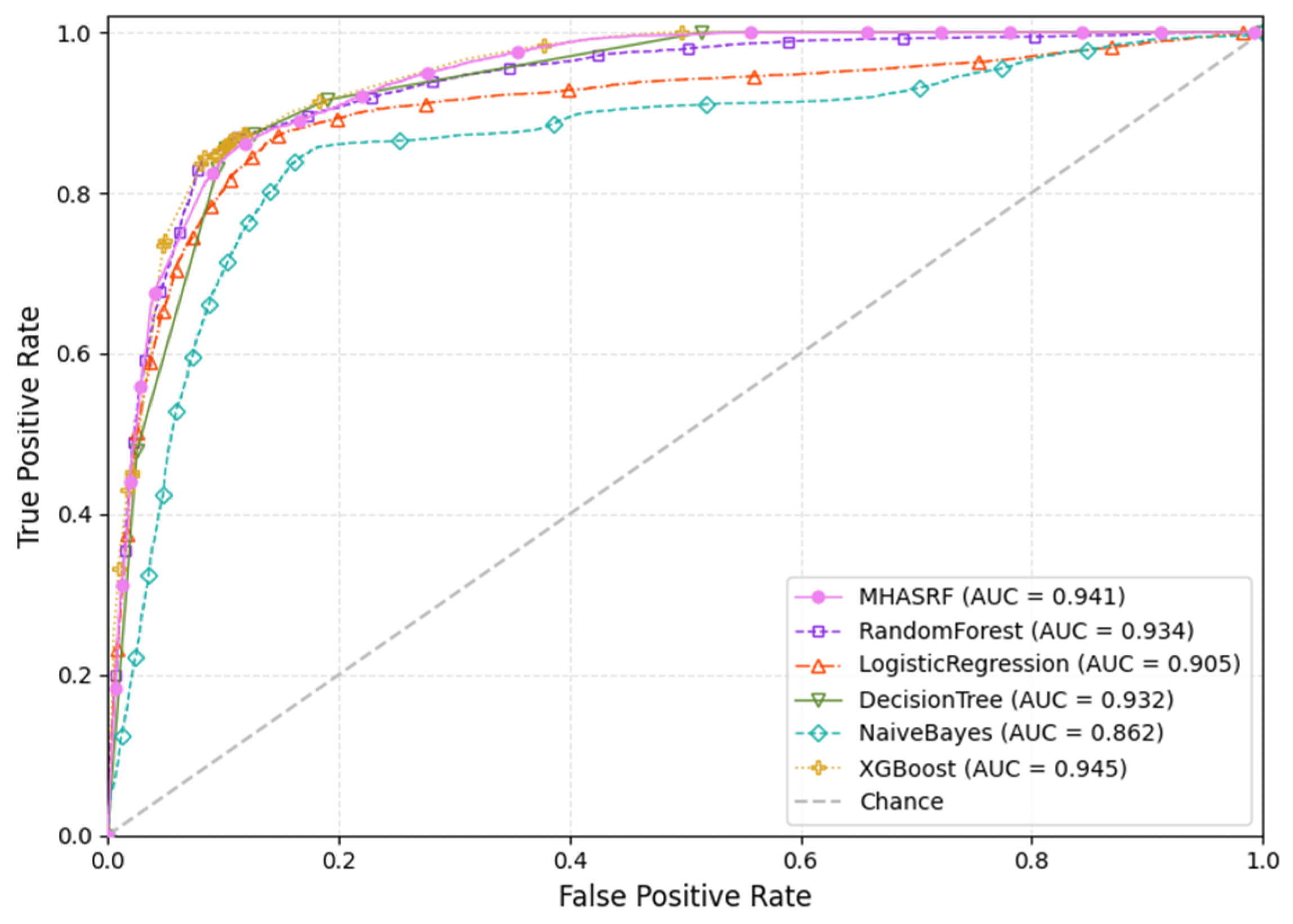
The predictive performance of the MHASRF and baseline models is compared using ROC curves in the held-out testing set in Figure 3. The AUC was largest for the XGBoost model (0.945), followed by the MHASRF model (0.941), both of which outperformed the RF (0.934) and DT (0.932) models. Thus, the MHASRF model maintained a strong overall ability to distinguish between TPs and TNs across different classification thresholds. Overall, the ROC curves support the conclusion that the MHASRF model performs competitively on the held-out testing set and shows well-balanced predictive performance, especially in terms of overall class discrimination.

To further assess whether the observed performance differences were statistically meaningful, we compared the MHASRF model with each baseline model on the held-out testing set using McNemar’s tests (

Table 4. Pairwise McNemar’s tests comparing the MHASRF model and the baseline models on the held-out testing set.

Model vs. MHASRF	Only MHASRF Model Correct	Only Other Model Correct	p-Value	Interpretation
RF	1425	801	<10−6	MHASRF significantly better
LR	689	368	<10−6	MHASRF significantly better
DT	453	502	0.120	No significant difference
NB	1525	480	<10−6	MHASRF significantly better
XGBoost	324	452	5.0 × 10−6	XGBoost significantly better

). The MHASRF model significantly outperformed RF, LR, and NB models (p < 0.05) but not the DT model (p = 0.120), indicating that the two models performed comparably. In contrast, the XGBoost model significantly outperformed the MHASRF model (p = 5.0 × 10⁻⁶), consistent with its higher accuracy, F₁-score, and AUC in the main performance analysis. Nevertheless, the MHASRF model remains a competitive alternative, particularly given its hybrid differentiable architecture of SDTs, instance-specific SDT weighting mechanism, and richer explanatory analysis through attention weights and dual-level feature importance. These characteristics make the MHASRF model a meaningful contribution beyond predictive accuracy alone.

4.2. Loss Curve Analysis

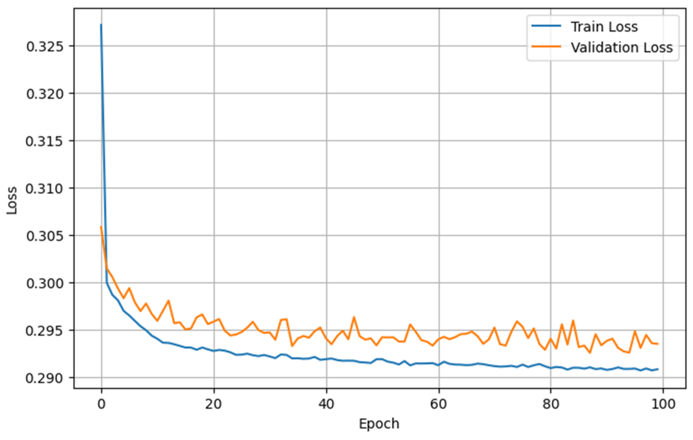
The average training and validation loss curves of the proposed MHASRF model are shown in Figure 4. The training loss decreased steadily and converged over the training epochs, indicating that the MHASRF model effectively learned from the training data. The validation loss also showed a generally decreasing trend and remained close to the training loss. The relatively small gap between the two curves suggests stable generalization performance and no clear sign of substantial overfitting.

4.3. Attention Weight Distribution

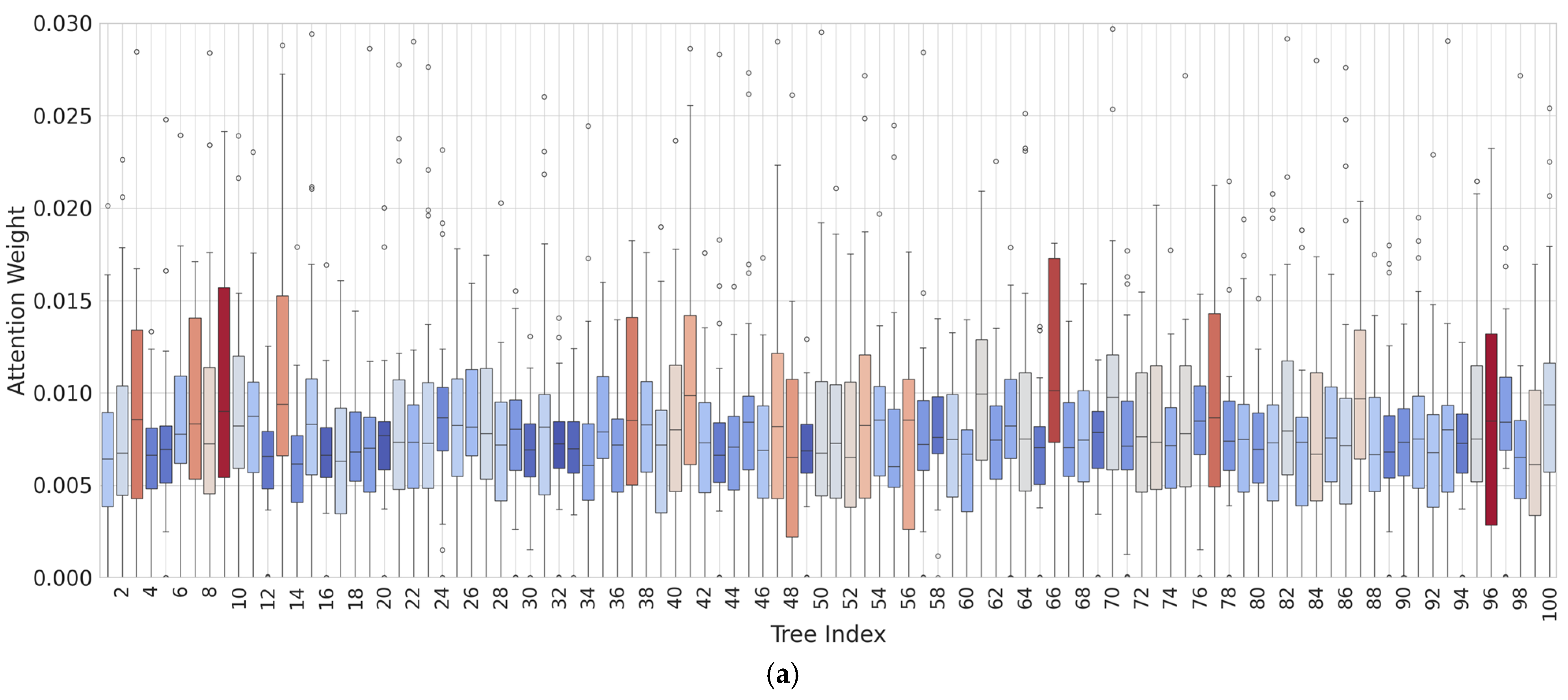
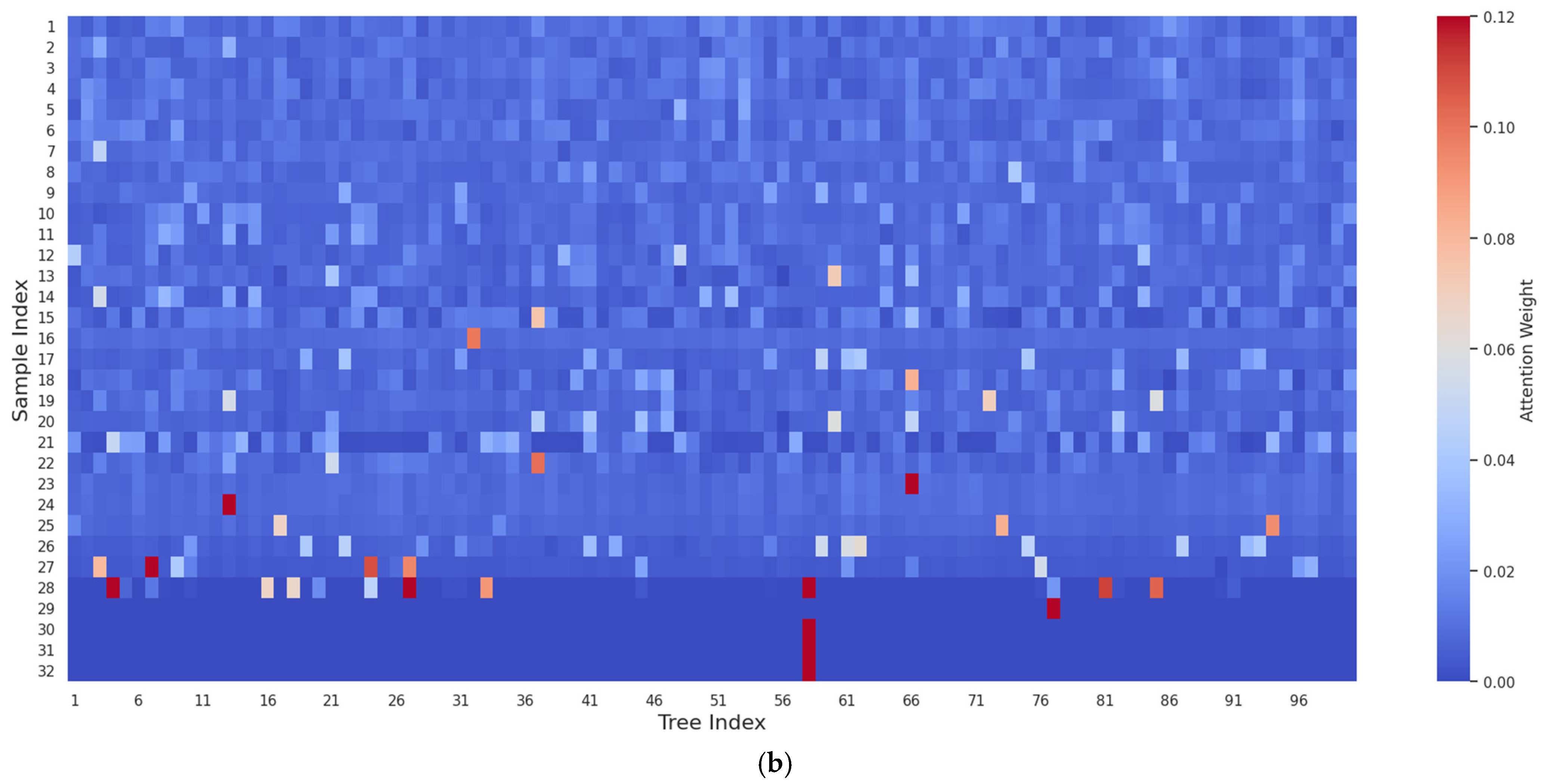
In this study, the attention mechanism is interpreted as a model-based weighting mechanism that reveals how the contribution of different SDTs varies across input instances, rather than as a direct causal explanation of patient no-show behavior. An example of the attention weights assigned to each SDT in the MHASRF model for a batch of 32 appointments is shown in Figure 5, revealing the dynamic behavior of SDT attention distribution across appointments. SDTs with relatively stable attention distributions across appointments may represent broader, more consistently useful decision patterns, whereas SDTs with more variable attention distributions may capture more specialized patterns relevant only to certain appointment profiles.

The distribution of attention weights for each SDT across the 32 appointments is shown in Figure 5a. The interquartile range (IQR) of each box plot reveals how consistently each SDT contributes across appointments. SDTs with short box plots (narrow IQRs), such as Trees 20, 32, and 49, exhibit tightly clustered distributions, indicating more stable attention weights across appointments. Thus, these SDTs contribute similarly in most predictions. In contrast, SDTs with long box plots (broad IQRs), such as Trees 10, 66, and 96, show greater variability in attention weights across appointments, indicating that their contributions depend more strongly on the characteristics of the particular appointment.

How attention is distributed per SDT per appointment is visualized as a heat map in Figure 5b, with the SDT index on the x-axis and the appointment index on the y-axis. The distribution of attention is not uniform: some SDTs are highly weighted only for specific subsets of appointments, while others are not weighted at all. For instance, Trees 4, 7, and 58 might carry more weight for certain appointments than for others. This pattern is consistent with the intended behavior of the proposed attention mechanism, which assigns instance-specific weights to SDT outputs. From a modeling perspective, this pattern suggests that the MHASRF model does not rely on a single fixed decision rule for all appointments; instead, it adapts the relative influence of SDTs based on appointment-specific information.

These visualizations collectively demonstrate that the attention mechanism in the MHASRF model allows for instance-specific SDT weighting and adapts its internal decision process across cases. This adaptation makes the MHASRF model more flexible and suitable for predicting patient no-shows in real healthcare settings, where behavior can vary substantially across patients and appointment contexts. Instead of giving equal weight to all SDTs, the MHASRF model learns to focus on different SDTs depending on the input. This adaptive weighting may help capture heterogeneous patterns in patient no-show behavior and provide an informative view of how the MHASRF model responds to different appointment profiles. However, the attention distribution should be interpreted as a complementary explanation of model behavior rather than as direct evidence of the real-world causes of patient no-shows. In this sense, the attention mechanism enhances the MHASRF model’s explanatory power while remaining aligned with the structured and interpretable nature of tree-based modeling.

4.4. Feature Importance Analysis

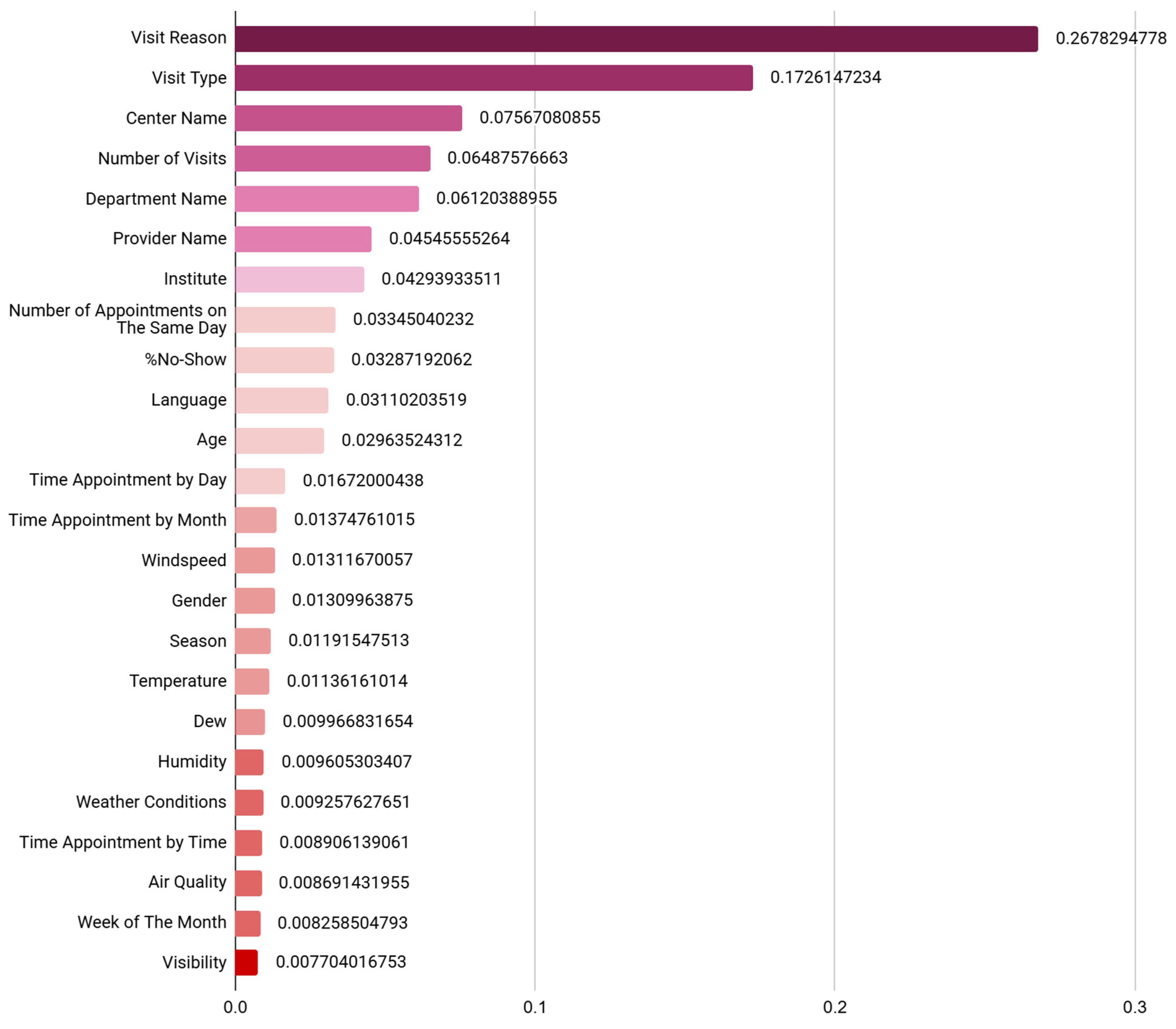
In addition to the instance-specific patterns discussed above, we further examined the MHASRF model’s behavior by analyzing the relative importance of the input features. This analysis provides a global summary of which features contribute most strongly to its predictions. The normalized final feature importance scores obtained from the MHASRF model are shown in Figure 6. These plotted values correspond to the final combined importance score for each feature, computed by integrating tree-level and attention-level importance scores, as defined in Equations (11)–(13). The two importance scores were first normalized separately and then averaged with equal weights to obtain the final score.

Appointment-related factors such as Visit Reason (26.78%) and Visit Type (17.26%) had the highest importance scores, highlighting that the purpose and type of the scheduled appointment play a major role in whether a patient attends. Contextual and organizational features, including Center Name (7.57%), Department Name (6.12%), Provider Name (4.55%), and Institute (4.29%), also ranked highly, indicating that attendance behavior may be influenced not only by patient history but also by the clinical setting in which the appointment is scheduled. One possible explanation is that these features reflect differences in clinic operations, such as scheduling practices, patient mix, workflow, or provider-related patterns. Therefore, they may be important not only as individual predictors, but also because they represent broader operational conditions associated with patient no-shows.

History-based features, such as Number of Visits (6.49%), Number of Appointments on the Same Day (3.35%), and %No-show (3.29%), were also among the more influential predictors. These findings indicate that prior patterns remain relevant for predicting future no-show behavior. Overall, the results suggest that patient no-show prediction in our dataset is shaped by a combination of appointment characteristics, prior attendance behavior, and provider- or center-related context.

The results are partly consistent with previous studies that identified appointment history and visit-related features as important predictors of patient no-show [6,10,26,31]. However, our MHASRF model also identifies additional influential factors that have received less attention in prior research, including Center Name, Institute, and Department Name. These findings suggest that it can effectively capture feature importance in a manner consistent with other feature selection methods while also identifying previously underexplored features that may be relevant to predicting patient no-shows in real-world healthcare settings.

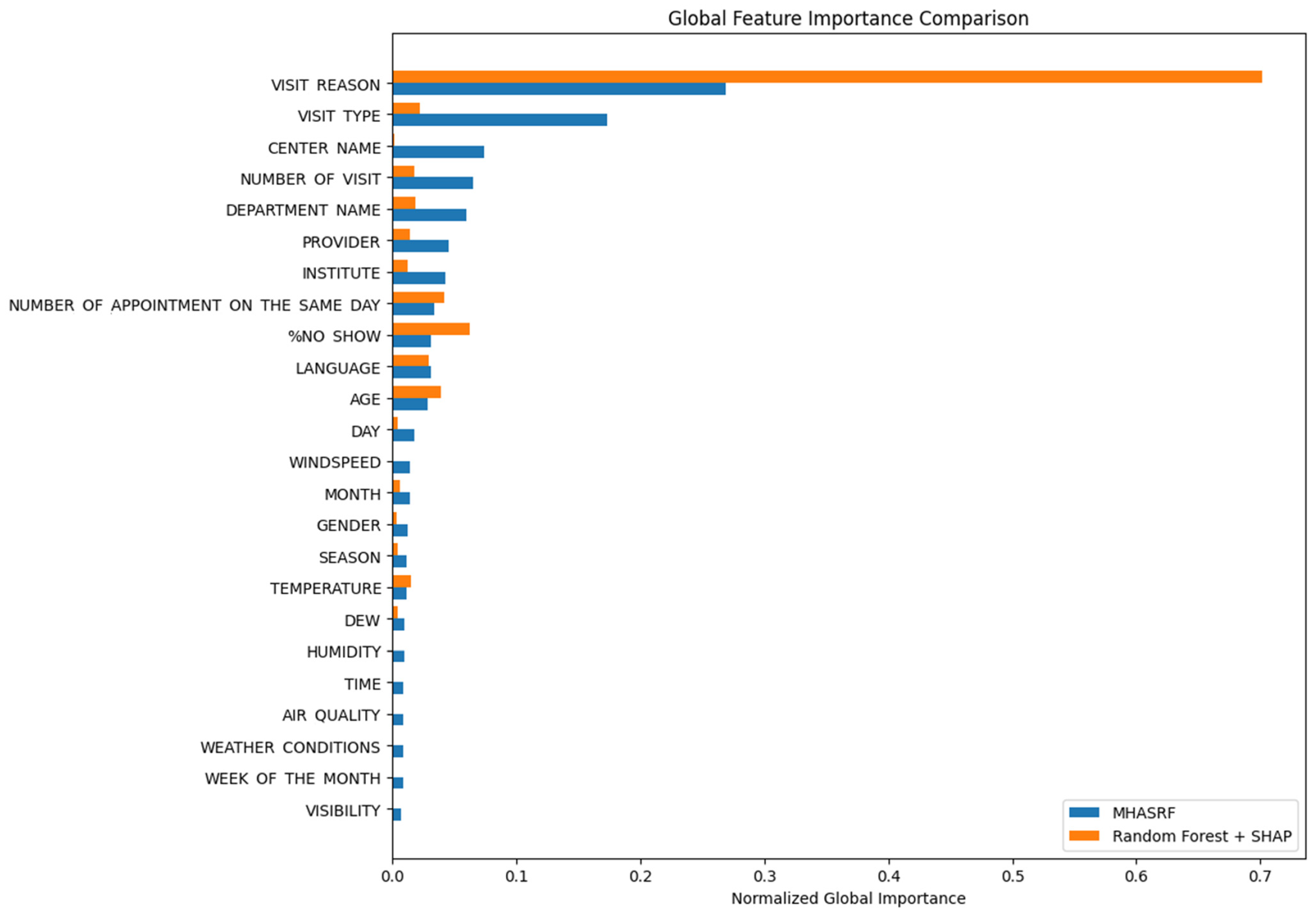
To further contextualize the feature-importance results, we compared the global importance ranking produced by the MHASRF model with a Shapley additive explanations (SHAP)-based global explanation from a conventional RF model (Figure 7). Both models identified Visit Reason as the most influential predictor, suggesting agreement on the main appointment-related driver of patient no-show behavior. Beyond this common finding, the two models differed in how importance was distributed across the remaining features. In particular, the SHAP-based RF model explanation assigned substantial importance to Visit Reason. In contrast, the MHASRF model assigned importance more dispersedly across appointment-related, history-based, and contextual features. This more distributed pattern may result from the MHASRF model’s importance calculation, which combines tree-level importance with attention-based tree weighting. Therefore, a feature can be assigned higher importance when it has a strong contribution within SDTs that also receive high attention weights. Beyond Visit Reason, the SHAP-based RF model explanation assigned greater importance to features such as %No-show, Number of Appointments on the Same Day, and Age, whereas the MHASRF model assigned relatively greater importance to contextual features, such as Center Name, Department Name, Provider Name, and Institute.

The observed differences between approaches likely reflect their distinct model structures and explanation mechanisms. Although both approaches summarize feature relevance after model training (post hoc explanation), they are derived differently. The SHAP-based RF model explanations provide a post hoc feature-attribution view from the RF model. In contrast, the MHASRF model computes feature importance from the trained model’s internal components by combining tree-level importance and attention-level tree weighting. Therefore, this comparison should be interpreted as qualitative rather than quantitative. In addition, Figure 5 provides a local view of the MHASRF model’s attention mechanism by showing how attention weights are distributed across SDTs for individual patient appointments. This local attention analysis illustrates how the MHASRF model adaptively changes the contribution of different SDTs across cases, but it should not be interpreted as local feature-level attribution. Thus, the MHASRF model provides global feature-importance information and instance-specific tree-weighting behavior, while the SHAP-based RF model explanations are feature-attribution-based; the two should be viewed as complementary rather than directly comparable.

4.5. Ablation Study

We conducted an ablation study to examine the impact of each model component. The contributions of key components of the MHASRF model are illustrated in

Table 5. Ablation study results.

Model	Accuracy	Specificity	Precision	Recall	F1-Score	AUC
SHASRF	88.08%	91.17%	81.46%	81.59%	81.52%	93.90%
MHASRF (2-head)	88.16%	90.71%	80.91%	82.81%	81.85%	93.99%
MHASRF (3-head)	88.24%	91.21%	81.60%	82.01%	81.81%	94.07%
MHASRF (4-head)	88.03%	90.36%	80.35%	83.15%	81.75%	93.81%
MHASRF (8-head)	88.08%	90.15%	80.17%	83.71%	81.90%	93.95%
MHASRF (without δk)	88.15%	91.06%	81.35%	82.06%	81.70%	94.08%

Abbreviations: SHASRF, single-attention-head soft random forest.

. Overall, the MHASRF model demonstrated competitive and stable performance across different attention-head configurations. Among all tested models, the 3-attention-head MHASRF model demonstrated the best overall balance, with an accuracy of 88.24%, specificity of 91.21%, precision of 81.60%, recall of 82.01%, F₁-score of 81.81%, and AUC of 94.07%. Although it did not achieve the highest recall or F₁-score, its performance across metrics indicates that the 3-attention-head configuration offers the most balanced trade-off between maximizing TPs and controlling FPs.

The baseline single-attention-head SRF (SHASRF) model achieved an accuracy of 88.08%, specificity of 91.17%, precision of 81.46%, recall of 81.59%, F₁-score of 81.52%, and AUC of 93.90%. Replacing the single attention head with multiple attention heads generally improved recall and F₁-score. The two-attention-head MHASRF model achieved an accuracy of 88.16%, specificity of 90.71%, precision of 80.91%, recall of 82.81%, F₁-score of 81.85%, and AUC of 93.99%. In contrast, the four-attention-head MHASRF model achieved an accuracy of 88.03%, specificity of 90.36%, precision of 80.35%, recall of 83.16%, F₁-score of 81.75%, and AUC of 93.81%. Moreover, the eight-attention-head MHASRF model achieved an accuracy of 88.08%, specificity of 90.15%, precision of 80.17%, the highest recall of 83.71%, the highest F₁-score of 81.90%, and an AUC of 93.95%.

The comparison across different numbers of attention heads reveals a clear trade-off: increasing the number of heads beyond three tends to improve recall, but reduce specificity and precision. For example, the four- and eight-attention-head MHASRF models achieved higher recall than the three-attention-head MHASRF model, indicating that they could identify more TPs. However, this improvement came at the cost of lower precision. Therefore, while the eight-attention-head MHASRF model achieved the highest recall and F₁-score, the three-attention-head MHASRF model remains the most balanced because it achieved the highest accuracy, specificity, precision, and one of the highest AUCs.

We also examined the role of the trainable tree reliability parameter, δ_k(x), by removing it from the MHASRF architecture. The model without δ_k(x) achieved an accuracy of 88.15%, specificity of 91.06%, precision of 81.35%, recall of 82.06%, F₁-score of 81.70%, and the highest AUC of 94.08%. Although this configuration obtained a slightly higher AUC than the three-attention-head MHASRF model, the model without δk(x) showed slightly lower accuracy, specificity, precision, and F₁-score. Thus, the tree reliability parameter helps improve overall classification balance, even though it has only a minor effect on the AUC.

The tree reliability parameter plays a crucial role in adjusting the attention weights assigned to individual SDTs. SDTs with consistently high classification errors are assigned lower attention weights, thereby preventing unreliable SDTs from exerting excessive influence on the final prediction. Unlike traditional RFs that assign the same weight to all trees, our approach actively mitigates the impact of weak and irrelevant SDTs. Removing the tree reliability parameter resulted in a slight decline in performance, confirming that weighting SDTs based on reliability reduces the influence of poorly performing SDTs.

Replacing multi-head attention with a single-head attention resulted in a modest reduction in performance; however, the three-attention-head MHASRF model consistently achieved higher recall and F₁-score than the SHASRF model, indicating that multi-head attention helped the model capture a broader range of patterns related to patient no-show behavior. However, the improvements are not large, with AUCs in a narrow range of 93.8–94.1%. Thus, the MHASRF proposed architecture was already strong, and the contribution of multi-head attention appeared to primarily improve the balance between precision and recall.

In real-world settings, patients miss appointments for various reasons. By employing multiple attention heads, the MHASRF model can simultaneously focus on different behavioral patterns. Therefore, even though the performance gains are modest, multi-head attention remains beneficial, as it improves the balance between competing prediction objectives and enhances the model’s flexibility for real-world clinical settings.

4.6. Stratified Analysis by Department

To further examine the MHASRF model’s behavior across clinical settings, we conducted a stratified analysis by department in the held-out testing set (

Table 6. Stratified department-level analysis of MHASRF model performance and predicted patient no-show rates in the held-out testing set.

Department	Number of Appointments	Actual No-Shows	Predicted No-Shows	Actual No-Show Rate	Predicted No-Show Rate	Prediction Difference	PPV	NPV
Colorectal surgery	1085	301	250	27.74%	24.70%	−0.0304	94.80%	92.34%
Dentistry	1285	406	353	31.60%	27.88%	−0.0371	77.05%	85.62%
Gastroenterology	6837	2302	2200	33.67%	33.10%	−0.0057	92.55%	94.26%
General surgery	2889	796	811	27.55%	28.78%	0.0122	81.26%	93.41%
Gynecology	80	12	20	15.00%	20.37%	0.0537	60.00%	100.00%
Nutrition	1139	527	908	46.27%	65.19%	0.1892	53.08%	80.52%
Otolaryngology	3068	1051	931	34.26%	33.17%	−0.0109	89.69%	89.89%
Plastic surgery	367	145	102	39.51%	32.44%	−0.0707	93.14%	81.13%
Speech therapy	228	74	163	32.46%	66.48%	0.3402	38.04%	81.54%
Urology	3080	877	846	28.47%	28.46%	−0.0002	81.80%	91.72%
Wound care	414	107	19	25.85%	18.37%	−0.0748	52.63%	75.44%

). Its performance varied across departments, indicating that patient no-show behavior is not uniform across specialties. This subgroup analysis provides an additional perspective beyond the analysis of the entire testing set, showing where the model performs more consistently and where greater prediction error remains.

In several departments with larger numbers of appointments, the predicted patient no-show rate closely matched the observed rate. For instance, in gastroenterology, the actual patient no-show rate was 33.67%, and the predicted rate was 33.10%, a small difference of −0.57%. A similar pattern was observed in urology, where the actual and predicted patient no-show rates were almost identical (28.47% vs. 28.46%). In both departments, the PPV and NPV were also relatively high, suggesting that the MHASRF model performed in a stable and balanced manner.

A similar tendency was found in general surgery and otolaryngology. In general surgery, the MHASRF model slightly overpredicted, yet maintained a good PPV (81.26%) and a high NPV (93.41%). In otolaryngology, the predicted patient no-show rate (33.17%) was also close to the observed rate (34.26%), with both the PPV and NPV close to 0.90. These results suggest that the MHASRF model performs consistently in departments with larger appointment volumes.

In contrast, the MHASRF model showed larger discrepancies in several departments with smaller or more variable appointment volumes. In speech therapy, the predicted patient no-show rate (66.48%) was much higher than the observed rate (32.46%), resulting in the largest gap (+34.02%). This overprediction was accompanied by a low PPV (38.04%), meaning that many appointments predicted as no-shows were actually attended. A similar pattern appeared in nutrition, where the predicted patient no-show rate exceeded the actual rate by 18.92%. In gynecology, the predicted patient no-show rate was also higher than the observed rate (20.37% vs. 15.00%), although the sample size was relatively small. These results suggest that the MHASRF model may be more likely to overpredict patient no-shows in departments with lower appointment volumes or more heterogeneous patient attendance patterns.

Some departments showed the opposite pattern. In plastic surgery, wound care, and colorectal surgery, the predicted patient no-show rate was lower than the observed rate. For colorectal surgery, the gap was relatively small (−3.04%), and both the PPV (94.80%) and NPV (92.34%) were high, indicating strong performance despite slight underprediction. However, in plastic surgery and wound care, the gap was larger but still negative, suggesting that the model tended to underpredict patient no-shows in those departments.

Overall, these results show that our MHASRF model performs well in several major departments, while also revealing meaningful variation across specialties. It appears to behave more reliably in departments with larger appointment volumes, such as gastroenterology, urology, and otolaryngology, where the predicted and observed patient no-show rates closely matched, and both the PPV and NPV remained high. In contrast, larger differences were observed in departments such as speech therapy and nutrition, where the MHASRF model tended to overpredict patient no-shows and showed a relatively low PPV. Thus, patient no-show behavior in these departments appears more heterogeneous and may be shaped by more department-specific patterns that are not fully captured by the general predictors used in this study. This interpretation is also consistent with the feature-importance results (Figure 6), which identified department-related and organizational features, such as Department, Center, Provider, and Institute, as influential predictors. In addition, departments with smaller sample sizes may provide less stable learning signals than larger departments, potentially leading the MHASRF model to overidentify no-show cases in these settings.

From a practical perspective, these findings suggest that overall performance provides a useful summary of model behavior, while stratified analysis offers additional insight into how the model performs across departments. Therefore, the subgroup-level analysis adds value by showing where the MHASRF model performs more consistently and where further refinement may be beneficial. It also highlights the importance of department-level evaluation when considering real-world deployment. These results suggest that future work may benefit from department-aware calibration or adaptation strategies to further improve performance consistency across clinical contexts.

4.7. Contextual Comparison with Prior No-Show Prediction Studies

The performance of the MHASRF model is compared with that of the best-performing models for predicting patient no-shows in prior studies in

Table 7. Contextual comparison of the MHASRF model with the best-performing models for predicting patient no-shows in prior studies.

Study	Year	Clinical Setting	Best-Performing Model	Accuracy	AUC
Srinivas et al. [5]	2021	Cardiology clinic	GB	–	85.00%
Hamdan et al. [22]	2022	Outpatient hospital	GB	78.00%	65.00%
Abushaaban et al. [29]	2022	Multiple hospitals	Symbolic regression and instance hardness threshold	94.00%	94.00%
Valero-Bomer et al. [10]	2022	Outpatient hospital	DT	73.00%	–
Liu et al. [14]	2022	Pediatric hospital	DNN		97.00%
Dustan et al. [11]	2023	Pediatric hospital (multi-specialty)	Balanced ensemble methods	–	71–83%
Almutairi et al. [8]	2024	Dental appointments	DT	80.00%	84.00%
This Study	2025	Outpatient hospital	MHASRF	88.24%	94.07%

Abbreviations: DNN, deep neural network; DT, decision tree; GB, gradient boosting; MHASRF, multi-head attention soft random forest.

. This comparison of accuracy and AUC helps contextualize the MHASRF model’s performance.

The results suggest that the MHASRF model is competitive with many previously reported models, achieving an accuracy of 88.24% and an AUC of 94.07%. In particular, its AUC is higher than that of several earlier models tested in cardiology, dental, and general outpatient settings. However, some prior models performed better [14,29]. Notably, these comparisons should be interpreted cautiously because the studies differ in clinical setting, dataset composition, patient population, feature availability, and evaluation protocol. Nevertheless, these results suggest that the MHASRF model offers competitive predictive performance while also contributing a distinct hybrid framework for predicting patient no-shows.

4.8. Tree-Wise Attention and the Structure of Appointment Data

The MHASRF model employs a tree-wise attention mechanism rather than a sequence-wise attention model. We made this choice because we conceptualized this study as an appointment-level prediction task, where each instance corresponds to a single appointment represented by structured features. Although the data contain a longitudinal aspect, this temporal information was incorporated through history-based features such as %No-show and Number of Visits, rather than through the full sequence of appointments.

In contrast, a sequence-based attention model would require each patient’s complete appointment history to be arranged temporally so that the model could learn directly from the sequence of prior visits. Thus, it represents a different modeling approach with different requirements for data representation and interpretation. Sequence-based models also require patient histories to be represented explicitly as temporal sequences and generally benefit from larger datasets for stable training. Moreover, the interpretability of sequence-based and tree-based models differs depending on the specific architecture and explanation methods used. In this study, the proposed tree-based approach was considered more suitable because it aligns well with the structured tabular nature of the data and provides interpretable model components through its tree-level structure, tree-wise attention weights, and global feature importance analysis. Therefore, MHASRF is an appointment-level prediction model that uses historical information rather than a model that directly learns from the full temporal sequence of appointments. Nevertheless, sequence-based models remain an important direction for future research.

5. Limitations and Future Directions

This study has several limitations that should be acknowledged. Firstly, the dataset was obtained from a single healthcare provider in the Middle East and covered one year of appointments, which may limit the generalizability of our findings to other institutions and populations. Secondly, the proposed MHASRF model was formulated as an appointment-level prediction model that uses history-based features rather than full temporal appointment sequences. Thirdly, the stratified analysis showed that the MHASRF model’s behavior varied across departments, especially in those with smaller or more variable appointment volumes. Fourthly, although the MHASRF model showed competitive and balanced performance, the XGBoost model performed better overall across several summary metrics, indicating that the proposed MHASRF model’s main advantage lies not only in prediction but also in interpretability and analytical richness. Fifthly, some derived contextual and environmental features, such as outside temperature, humidity, visibility, and air quality, may be specific to the study setting. Moreover, these variables may not be available in the same form or may not have the same predictive relevance in other healthcare systems, regions, or climates.

Future research should evaluate the MHASRF model on external multi-hospital datasets and across longer time periods to assess its generalizability. It should also explore department-aware calibration, sequence-based modeling using full appointment histories, and the inclusion of additional access-related features, such as travel distance, reminder information, and transportation factors. Moreover, it should examine the availability of contextual and environmental features, such as weather and air quality, across different healthcare settings. Finally, prospective studies are also needed to determine whether the MHASRF model’s interpretability and balanced predictive profile translate into measurable operational benefits in real scheduling practice.

6. Conclusions

This study proposed a hybrid MHASRF model for predicting patient no-shows that integrates an SRF with multi-head attention and trainable tree-reliability weighting. The proposed framework combines probabilistic soft splits with instance-specific tree weighting, allowing the model to retain the robustness and interpretability of tree-based learning while introducing adaptive attention across trees. Compared with baseline models (DT, RF, LR, NB, and XGBoost), the MHASRF model achieved competitive and well-balanced predictive performance on structured healthcare data.

In the held-out testing set, the MHASRF model achieved an accuracy of 88.24%, specificity of 91.21%, recall of 82.01%, precision of 81.60%, NPV of 91.42%, F₁-score of 81.81%, and AUC of 94.07%. Although the XGBoost model performed the best overall across several summary metrics, the MHASRF model remained competitive and demonstrated a favorable balance across evaluation measures, particularly in terms of specificity, precision, and overall interpretability. These findings suggest that integrating attention mechanisms into tree-based models can provide a meaningful alternative for structured healthcare prediction tasks where both predictive performance and model transparency are important.

In addition, the proposed MHASRF model provides richer explanatory analysis through dual-level importance at both the tree and attention levels. Visit reason, visit type, and prior attendance-related features were among the most influential predictors, while contextual features such as department, center, provider, and institute also played an important role. These findings indicate that patient no-show behavior is shaped not only by appointment characteristics and attendance history but also by the broader organizational setting in which care is delivered.

However, this study had several limitations. Firstly, the model was developed using data from a single healthcare provider and was formulated as an appointment-level prediction model rather than a full sequence-based approach, which may limit its generalizability across institutions and clinical settings. Secondly, the stratified analysis showed that model performance differed across clinical specialties, suggesting that the current set of predictors may not fully capture specialty-specific patterns. Therefore, future research should examine external validation on multi-institutional datasets, department-aware calibration, and sequence-based extensions that incorporate longitudinal appointment histories. Overall, the MHASRF model offers a novel, interpretable, and competitive framework for predicting patient no-shows and provides useful insights into the complex factors associated with missed appointments.

References

1. Mazaheri Habibi, M.R.; Abadi, F.M.; Tabesh, H.; Vakili-arki, H.; Abu-Hanna, A.; Ghaddaripouri, K.; Eslami, S. Evaluation of no-show rate in outpatient clinics with open access scheduling system: A systematic review. Health Sci. Rep. 2024, 7, e2160. [Google Scholar] [CrossRef]
2. Kheirkhah, P.; Feng, Q.; Travis, L.M.; Tavakoli-Tabasi, S.; Sharafkhaneh, A. Prevalence, predictors and economic consequences of no-shows. BMC Health Serv. Res. 2016, 16, 13. [Google Scholar] [CrossRef]
3. Nguyen, D.L.; DeJesus, R.S.; Wieland, M.L. Missed Appointments in Resident Continuity Clinic: Patient Characteristics and Health Care Outcomes. J. Grad. Med. Educ. 2011, 3, 350–355. [Google Scholar] [CrossRef]
4. Drabkin, M.J.; Lobel, S.; Kanth, N.; Martynov, A.; Hunt, H.W.; Guerrero, D.; Fogel, J.; Grechanik, A.; Mancuso, C.D.; Lev, S. Telephone reminders reduce no-shows: A quality initiative at a breast imaging center. Clin. Imaging 2019, 54, 108–111. [Google Scholar] [CrossRef]
5. Srinivas, S.; Ravindran, A.R. Optimizing outpatient appointment system using machine learning algorithms and scheduling rules: A prescriptive analytics framework. Expert Syst. Appl. 2018, 102, 245–261. [Google Scholar] [CrossRef]
6. Dantas, L.F.; Hamacher, S.; Oliveira, F.L.C.; Barbosa, S.D.J.; Viegas, F. Predicting Patient No-show Behavior: A Study in a Bariatric Clinic. Obes. Surg. 2019, 29, 40–47. [Google Scholar] [CrossRef]
7. Ding, X.; Gellad, Z.F.; Mather, C.; Barth, P.; Poon, E.G.; Newman, M.; Goldstein, B.A. Designing risk prediction models for ambulatory no-shows across different specialties and clinics. J. Am. Med. Inform. Assoc. 2018, 25, 924–930. [Google Scholar] [CrossRef] [PubMed]
8. Almutairi, T.H.; Olatunji, S.O. The utilization of AI in healthcare to predict no-shows for dental appointments: A case study conducted in Saudi Arabia. Inform. Med. Unlocked 2024, 46, 101472. [Google Scholar] [CrossRef]
9. Ferro, D.B.; Brailsford, S.; Bravo, C.; Smith, H. Improving healthcare access management by predicting patient no-show behaviour. Decis. Support Syst. 2020, 138, 113398. [Google Scholar] [CrossRef]
10. Valero-Bover, D.; González, P.; Carot-Sans, G.; Cano, I.; Saura, P.; Otermin, P.; Garcia, C.; Gálvez, M.; Lupiáñez-Villanueva, F.; Piera-Jiménez, J. Reducing non-attendance in outpatient appointments: Predictive model development, validation, and clinical assessment. BMC Health Serv. Res. 2022, 22, 451. [Google Scholar] [CrossRef] [PubMed]
11. Dunstan, J.; Villena, F.; Hoyos, J.P.; Riquelme, V.; Royer, M.; Ramírez, H.; Peypouquet, J. Predicting no-show appointments in a pediatric hospital in Chile using machine learning. Health Care Manag. Sci. 2023, 26, 313–329. [Google Scholar] [CrossRef] [PubMed]
12. Alshammari, A.; Almalki, R.; Alshammari, R. Developing a predictive model of predicting appointment no-show by using machine learning algorithms. J. Adv. Inf. Technol. 2021, 12, 234–239. [Google Scholar] [CrossRef]
13. Alshammari, R.; Daghistani, T.; Alshammari, A. The Prediction of Outpatient No-Show Visits by Using Deep Neural Network from Large Data. Int. J. Adv. Comput. Sci. Appl. 2020, 11, 533–539. [Google Scholar] [CrossRef]
14. Liu, D.; Shin, W.Y.; Sprecher, E.; Conroy, K.; Santiago, O.; Wachtel, G.; Santillana, M. Machine learning approaches to predicting no-shows in pediatric medical appointment. npj Digit. Med. 2022, 5, 50. [Google Scholar] [CrossRef]
15. Chaudhari, S.; Mithal, V.; Polatkan, G.; Ramanath, R. An Attentive Survey of Attention Models. ACM Trans. Intell. Syst. Technol. 2021, 12, 53. [Google Scholar] [CrossRef]
16. Montavon, G.; Samek, W.; Müller, K.R. Methods for interpreting and understanding deep neural networks. Digit. Signal Process. 2018, 73, 1–15. [Google Scholar] [CrossRef]
17. Kuo, C.Y.; Yu, L.C.; Chen, H.C.; Chan, C.L. Comparison of models for the prediction of medical costs of spinal fusion in Taiwan diagnosis-related groups by machine learning algorithms. Healthc. Inform. Res. 2018, 24, 29–37. [Google Scholar] [CrossRef]
18. Li, J.; Shi, J.; Chen, J.; Du, Z.; Huang, L. Self-attention random forest for breast cancer image classification. Front. Oncol. 2023, 13, 1043463. [Google Scholar] [CrossRef]
19. Utkin, L.V.; Konstantinov, A.V. Attention-based random forest and contamination model. Neural Netw. 2022, 154, 346–359. [Google Scholar] [CrossRef] [PubMed]
20. Frosst, N.; Hinton, G. Distilling a Neural Network Into a Soft Decision Tree. arXiv 2017, arXiv:1711.09784. [Google Scholar] [CrossRef]
21. Breiman, L. Random Forests. Mach. Learn. 2001, 45, 5–32. [Google Scholar] [CrossRef]
22. AlMuhaideb, S.; Alswailem, O.; Alsubaie, N.; Ferwana, I.; Alnajem, A. Prediction of hospital no-show appointments through artificial intelligence algorithms. Ann. Saudi Med. 2019, 39, 373–381. [Google Scholar] [CrossRef]
23. Ahmad, M.U.; Zhang, A.; Mhaskar, R. A predictive model for decreasing clinical no-show rates in a primary care setting. Int. J. Healthc. Manag. 2021, 14, 829–836. [Google Scholar] [CrossRef]
24. Batool, T.; Abuelnoor, M.; El Boutari, O.; Aloul, F.; Sagahyroon, A. Predicting Hospital No-Shows Using Machine Learning. In Proceedings of the IoTaIS 2020—Proceedings: 2020 IEEE International Conference on Internet of Things and Intelligence Systems; Institute of Electrical and Electronics Engineers Inc.: New York, NY, USA, 2021; pp. 142–148. [Google Scholar] [CrossRef]
25. Goffman, R.M.; Harris, S.L.; May, J.H.; Milicevic, A.S.; Monte, R.J.; Myaskovsky, L.; Rodriguez, K.L.; Tjader, Y.C.; Vargas, D.L. Modeling patient no-show history and predicting future outpatient appointment behavior in the veterans health administration. Mil. Med. 2017, 182, e1708–e1714. [Google Scholar] [CrossRef]
26. Topuz, K.; Uner, H.; Oztekin, A.; Yildirim, M.B. Predicting pediatric clinic no-shows: A decision analytic framework using elastic net and Bayesian belief network. Ann. Oper. Res. 2018, 263, 479–499. [Google Scholar] [CrossRef]
27. Mohammadi, I.; Wu, H.; Turkcan, A.; Toscos, T.; Doebbeling, B.N. Data Analytics and Modeling for Appointment No-show in Community Health Centers. J. Prim. Care Community Health 2018, 9, 2150132718811692. [Google Scholar] [CrossRef]
28. Hamdan, A.F.A.; Bakar, A.A. Machine Learning Predictions on Outpatient No-Show Appointments in a Malaysia Major Tertiary Hospital. Malays. J. Med. Sci. 2023, 30, 169–180. [Google Scholar] [CrossRef]
29. Abushaaban, E.; Agaoglu, M. Medical Appointment No-Show Prediction Using Machine Learning Techniques. In Proceedings of the 2022 2nd International Conference on Computing and Machine Intelligence, ICMI 2022—Proceedings; Institute of Electrical and Electronics Engineers Inc.: New York, NY, USA, 2022. [Google Scholar] [CrossRef]
30. Fan, G.; Deng, Z.; Ye, Q.; Wang, B. Machine learning-based prediction models for patients no-show in online outpatient appointments. Data Sci. Manag. 2021, 2, 45–52. [Google Scholar] [CrossRef]
31. Ahmadi, E.; Garcia-Arce, A.; Masel, D.T.; Reich, E.; Puckey, J.; Maff, R. A metaheuristic-based stacking model for predicting the risk of patient no-show and late cancellation for neurology appointments. IISE Trans. Healthc. Syst. Eng. 2019, 9, 272–291. [Google Scholar] [CrossRef]
32. Bahdanau, D.; Cho, K.; Bengio, Y. Neural Machine Translation by Jointly Learning to Align and Translate. arXiv 2014, arXiv:1409.0473. [Google Scholar]
33. Nadaraya, E.A. On Estimating Regression. Available online: https://www.mathnet.ru/eng/tvp356 (accessed on 14 May 2026).
34. Watson, G.S. Smooth regression analysis. Sankhya Ser. A 1961–2002 1961, 26, 359–372. [Google Scholar]
35. Vaswani, A.; Shazeer, N.; Parmar, N.; Uszkoreit, J.; Jones, L.; Gomez, A.N.; Kaiser, Ł.; Polosukhin, I. Attention Is All You Need. arXiv 2017, arXiv:1706.03762. [Google Scholar]
36. Utkin, L.V.; Konstantinov, A.V.; Kirpichenko, S.R. Attention and self-attention in random forests. Prog. Artif. Intell. 2023, 12, 257–273. [Google Scholar] [CrossRef]
37. Zhu, D.; Yao, H.; Jiang, B.; Yu, P. Negative Log Likelihood Ratio Loss for Deep Neural Network Classification. arXiv 2018, arXiv:1804.10690. [Google Scholar] [CrossRef]
38. Amalina, N.N. Prediction-Driven Adaptive Double-Booking Strategy for Outpatient Scheduling: A Multi-Objective Reinforcement Learning Approach. Master’s Thesis, Kumoh National Institute of Technology, Gumi, Republic of Korea, 2026. [Google Scholar]
Figure 1. The proposed framework. Abbreviations: AUC, area under the receiver operating characteristic curve; MHASRF, multi-head attention soft random forest; XGBoost, extreme gradient boosting.
Systems 14 00576 g001
Figure 2. Architecture of the MHASRF model.
Systems 14 00576 g002
Figure 3. Receiver operating characteristic (ROC) curves comparing model performance on the held-out testing set.
Systems 14 00576 g003
Figure 4. Training and validation loss curves for the MHASRF model.
Systems 14 00576 g004
Figure 5. Example attention weight distributions across SDTs for 32 patients. (a) Box plot showing the distribution of attention weight per SDT across appointments; (b) Heatmap showing attention weights per SDT for each appointment.
Systems 14 00576 g005aSystems 14 00576 g005b
Figure 6. Normalized final feature importance scores obtained from the MHASRF model.
Systems 14 00576 g006
Figure 7. Global feature comparison between the MHASRF model and a Shapley additive explanations (SHAP)-based RF model.
Systems 14 00576 g007