Dynamic Collection Routing Optimization for Domestic Waste with Mixed Fleets

Abstract

Influenced by factors such as residents’ living habits, commuting patterns, and commercial activity cycles, the generation of domestic waste exhibits a distinct double-peak distribution. To meet the high demand during peak periods, collection companies typically deploy excess transportation capacity, which leads to severe resource idleness during off-peak periods, imposing significant economic and environmental burdens. To address this issue, this study develops a dynamic smart waste collection routing model aimed at minimizing the coordinated collection cost between self-owned and outsourced multi-compartment vehicles, and designs a two-phase algorithm to solve it. In the pre-optimization phase, an improved Harris Hawks Optimization algorithm integrated with multiple heuristic algorithms is employed to generate initial collection routes. In the re-optimization phase, a hybrid strategy combining periodic and continuous re-optimization is used to dynamically update collection routes. Finally, the effectiveness of the proposed model and algorithm is validated through case studies. Furthermore, a systematic sensitivity analysis is conducted to investigate the impact of key parameters, yielding practical insights for waste collection management.

1. Introduction

Over recent decades, urban waste generation has surged worldwide due to population growth and rapid urbanization. The World Bank forecasts that global municipal solid waste will reach 3.4 billion tons by 2050 [1]. China, as the most populous country, generated 254 million tons of waste in 2024 [2]. Facing such challenges, waste management authorities must urgently develop effective and sustainable approaches to handle the growing volume of waste.

The entire waste management process mainly includes four stages: waste collection, waste transfer, secondary collection, and final disposal. Among them, waste collection and secondary collection are important issues because they account for 60–80% of the total cost of waste management [3]. Therefore, optimizing waste collection is not merely a logistics problem but a key entry point for improving the efficiency of the entire waste management process. It would not only reduce collection costs but also provide decision support for the optimal layout of waste facilities. As this study focuses on municipal waste collection, we ignored the subsequent waste processing procedures after the transfer station. Specifically, we focus on the collection process from waste collection points (WCPs) to the transfer station.

In response to the growing pressure on waste management, China’s central government has recently initiated a mandatory waste sorting policy, with Shanghai serving as the most representative city in its implementation [4]. It states that the waste collection system must be restructured from the traditional mixed collection model to a separate collection model that maintains waste sorting. Additionally, an innovative initiative known as “Removal of Bins and Consolidation of Points” is being implemented in most cities across China. This initiative aims to transform scattered bins into centralized waste collection points. Shanghai served as an early leader of this initiative, and other Chinese cities subsequently followed suit [5]. For example, Shanghai emphasizes a model combining centralized WCPs with fixed time slots and “green account” point incentives. Shenzhen has introduced smart devices at centralized WCPs accompanied by heavy fines, while Zhuhai relies on human supervision and guidance at such centralized WCPs. Although these cities have significant differences in their implementation models and intensities for this initiative, all of them have significantly reduced the number of WCPs, demonstrated that it is possible to achieve economies of scale in waste collection. This is a critical factor in waste collection, but it still faces barriers.

On the one hand, waste sorting is currently achieved by assigning dedicated vehicles to specific waste categories in most cities. Currently, separate vehicles are used for different waste types to keep waste sorted. However, this approach leads to multiple vehicle trips to the same site, raising collection costs and environmental burdens.

On the other hand, influenced by factors such as residents’ living habits, commuting patterns, and business activity cycles, the amount of domestic waste exhibits a distinct bimodal distribution pattern. Specifically, the amount of waste generated shows two distinct peaks during the morning and evening periods, creating a peak for collection demand. To cope with this heavy pressure, collection companies usually need to allocate excess transportation resources, including dispatching more vehicles, increasing the number of shifts, and extending working hours. However, this resource allocation model oriented towards peak demand leads to severe underutilization of collection capacity during off-peak hours. This brings considerable economic pressure to the sustainable operation of the collection companies and constitutes a critical challenge in waste collection operations.

To enhance resource utilization and collection efficiency, hybrid transportation capacity types combining self-operation, outsourcing and crowdsourcing has emerged in logistics practices. These types, which differ in working hours, shift scheduling practices, and compensation structures, can be strategically integrated to improve the overall efficiency of capacity resources. However, this study focuses on the collection of domestic waste. As a public service, it faces multiple risks such as uneven service coverage, illegal dumping and difficult supervision. Therefore, it is usually regulated and implemented by the government so it is characterized by a strong public character and a low degree of marketization. Therefore, this study does not consider the application of the crowdsourcing model in waste collection. In contrast, outsourced vehicles are usually not directly managed by government departments, which eliminates the costs associated with vehicle purchase and maintenance, thus effectively reducing fixed asset investments. Therefore, this study proposes a hybrid transport capacity model that combines self-operation and outsourcing as an optimal solution to enhance responsiveness and collection efficiency.

The waste collection problem is often regarded as a variant of the vehicle routing problem. In early studies, scholars mainly relied on historical data for analysis and seldom took real-time information into account [6,7,8]. The development of IoT technology, particularly smart waste bins, enabled real-time monitoring of waste fill levels, thereby supporting dynamic collection [9]. Hannan et al. [10] reviewed the existing information and communication technologies, analyzed their application in smart waste management, and discussed potential challenges. Subsequently, Hannan et al. [3] designed an improved particle swarm optimization algorithm for solid waste collection using smart waste bins. Akhtar et al. [11] established a mathematical model based on bin filling level thresholds to minimize total collection route distance. Nowakowski et al. [12] proposed a harmony search algorithm for recycling waste electrical and electronic equipment to optimize collection routes and validated its superiority through comparison with other algorithms. Idwan et al. [13] employed a two-stage heuristic algorithm to address the reverse logistics vehicle routing optimization problem for smart bins. They also conducted a comparative analysis between traditional and smart collection methods. Jorge et al. [14] adopted a hybrid meta-heuristic algorithm to prospectively determine which bins to collect based on their real-time and predicted filling levels. de Morais et al. [15] utilized real-time information on filling levels to construct a dynamic reverse inventory routing optimization model. Kim et al. [16] introduced two management methods to determine dynamic optimal routes. They combined ant colony optimization with the k-means clustering algorithm to solve the vehicle routing problem for large-scale waste collection. Although the above studies have considered dynamic collection scenarios, none of them addressed the vehicle routing problem when multiple types of waste in multi-compartment vehicles are involved. In the context of smart bin applications, Yang et al. [17] considered the uncertainty in waste generation rates and introduced a chance-constrained approach to solve a multi-compartment electric vehicle routing problem. Subsequently, Mohammadi et al. [18] first applied the discrete choice models to optimize dynamic multi-compartment vehicle routing problems, providing a new research perspective to the field. Despite these valuable contributions, neither study considered the impact of heterogeneous multi-compartment vehicles under dynamic demands in waste collection routing problems.

To the best of our knowledge, the existing studies on heterogeneous fleets in waste collection are predominantly framed within multi-level waste collection networks. Markov et al. [19] considered intermediate facilities and introduced a heterogeneous fleet and flexible destination allocation to address the recyclable waste collection problem. Asefi et al. [20] employed heterogeneous vehicles to construct a three-level collection network, aiming to optimize the fleet size and determine the optimal routes, thereby minimizing the waste collection cost. Ghiani et al. [21] focused on transfer stations in waste collection systems. The study indicated that waste was transferred from small vehicles to large ones at transfer stations. To address this, they proposed a two-stage optimization method to solve the routing problems of small and large vehicles. Cao et al. [22] focused on the electric vehicle routing problem in a two-level reverse logistics network. They adopted a heterogeneous hybrid fleet to reduce carbon emissions and save resources. Wei et al. [23] explored integrated optimization of a multi-level routing problem, aiming to plan a set of routes for manually driven vehicles and those equipped with compressors to minimize travel costs. Beyond the field of waste collection, heterogeneous fleets have been extensively adopted across diverse application domains. Nucamendi-Guillén et al. [24] studied a multi-depot location-routing problem with a heterogeneous fleet, aiming to minimize total costs by selecting contracted carriers, the types of vehicles used by each carrier, and the corresponding collection routes. Xu et al. [25] investigated the collaborative issue between ground vehicles and multiple drones and proposed a two-stage heuristic algorithm for its solution. Lin et al. [26] considered the optimization of task allocation and operational routing for a heterogeneous fleet of unmanned aerial vehicles to enable effective delivery of emergency medical services. While the majority of the above studies employed heterogeneous fleets for delivery tasks, they failed to systematically address the dynamic routing problem when both heterogeneous and multi-compartment vehicles are involved.

The introduction of heterogeneous vehicles and real-time changes in waste bin filling levels increase the complexity of the waste collection problem while also imposing higher requirements for the solution methods. Introduced by Heidari et al. [27], the Harris Hawks Optimization (HHO) algorithm is a recently developed metaheuristic algorithm. Its appeal stems from a lean parameter configuration, intuitive underlying mechanism, high implementation feasibility, and effective balance between exploration and exploitation. These attributes have facilitated its successful deployment in multiple fields [28,29,30]. Gupta et al. [31] improved the HHO algorithm using four strategies: a nonlinear energy formula, a greedy selection mechanism, opposition-based learning, and an attenuation factor. These improvements addressed the imbalance between exploration and exploitation. Nivethitha et al. [32] introduced an adaptive collaborative and decentralized foraging strategy in the HHO algorithm to guide the update of population positions. Fahmy et al. [33] improved the HHO algorithm by integrating an enhanced Chimpanzee Optimization Algorithm. They also proposed a new position update formula to calculate the prey’s escape energy. The above improvement strategies enhance the performance of the single HHO algorithm from multiple perspectives, including parameter tuning, population update mechanisms, and energy formula reformulation. However, such strategies are typically still confined to parameter or mechanism optimization within the HHO framework itself, making them prone to premature convergence to local optima. To overcome this limitation, researchers have begun exploring hybrid algorithms that combine multiple algorithms to break through the performance bottlenecks of single algorithms. Bao et al. [34] enhanced the search capability of HHO by adopting the differential evolution algorithm. This algorithm has been successfully applied to image segmentation, verifying its performance advantages. Sehgal et al. [35] combined the slime mold optimization algorithm with the HHO algorithm, thereby effectively avoiding convergence to local optima. Sharma et al. [36] constructed seven enhanced variants of the HHO algorithm. By incorporating adaptive parameter adjustment, chaotic mapping, elite individual retention, and multi-algorithm collaboration, these algorithms were designed to achieve a more effective balance between global exploration and local exploitation.

In summary, a significant research gap exists in the current research on smart waste collection. On the one hand, in both waste collection and other delivery domains, most models only consider single-compartment vehicles, multi-compartment vehicles, or heterogeneous vehicles in isolation. Few studies have simultaneously addressed the routing optimization of both multi-compartment and heterogeneous vehicles under dynamic demand. On the other hand, the existing algorithms struggle to balance global exploration and local exploitation when tackling complex optimization problems, making them prone to premature convergence and resulting in low search efficiency.

To address the aforementioned research gap, the main questions addressed by this study are as follows: (1) Under dynamic demand, how should we optimize the multi-compartment vehicle collection cost when using heterogeneous fleets? (2) In the face of dynamic collection requirements, how can efficient collection decisions be made in an extremely short time? (3) What are the sensitive parameters in this problem, and how do they affect the collection route planning?

Therefore, this study investigates the dynamic collection route optimization problem with multi-compartment vehicles in a mixed fleet of self-operated and outsourced vehicles. The main contributions are as follows:

• A two-stage model is constructed to minimize the dynamic collection cost of multi-compartment vehicles with heterogeneous fleets.
• To respond in a timely manner to collection demands, a hybrid strategy combining continuous and periodic optimization is designed. Meanwhile, a greedy insertion algorithm is adopted for local optimization, and an improved HHO algorithm is employed for global optimization. The improved HHO algorithm integrates multiple heuristic algorithms to ensure a balance between exploration and exploitation and avoid local optima.
• The validity of the proposed model and method is verified through case studies, and the sensitivity of key parameters is systematically analyzed. This provides a quantifiable decision-making basis and management implications for the dynamic collection of domestic waste.

The rest of this study is organized as follows. Section 2 describes the operational problems. In Section 3, we present the pre-optimization and re-optimization models. Section 4 elaborates on the design of the model solving algorithm. Numerical experiments are detailed in Section 5. Section 6 provides the sensitivity analysis. Finally, Section 7 is devoted to the conclusions and further work.

2. Problem Description

This study considers WCPs within residential areas, related transfer stations, and multi-compartment collection vehicles consisting of both self-owned and outsourced fleets. In China, domestic waste is classified into four categories: kitchen waste, recyclable waste, hazardous waste and other waste. Recyclable waste and hazardous waste each have their own specialized collection systems, and thus are not considered in this study.

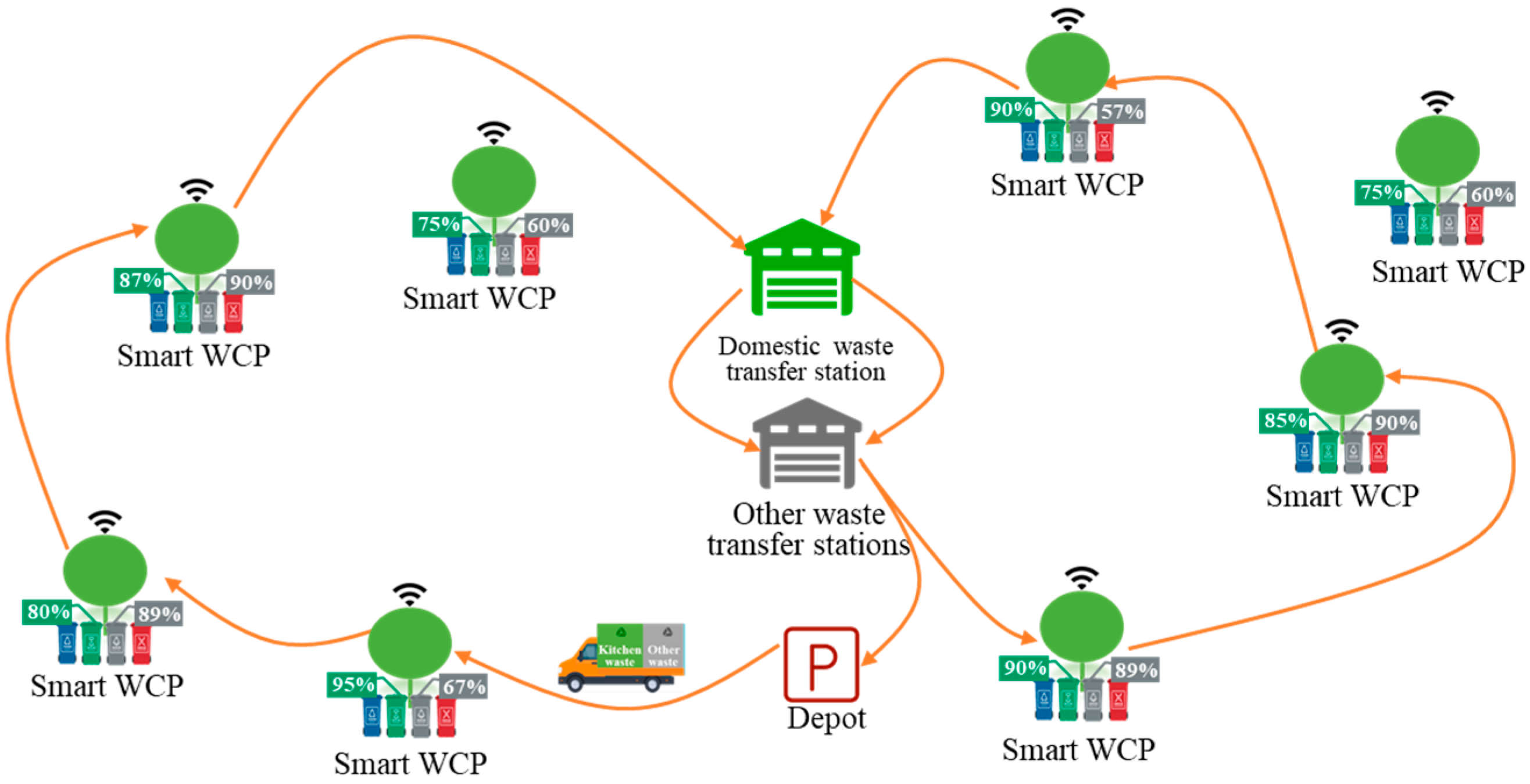
The problem can be described as shown in Figure 1. A two-compartment waste collection vehicle departs from the depot every day and sequentially visits WCPs that have reached the collection threshold to collect kitchen waste and other waste. When any compartment cannot accommodate additional waste, the vehicle will go to the nearest waste transfer station corresponding to that waste type to unload. It then continues collecting waste at the remaining WCPs until all waste is gathered. Following this, the vehicle sequentially unloads at both transfer stations and then returns to the depot. Each WCP must be served by exactly one vehicle.

Influenced by residents’ commuting and daily routines, the amount of waste generated at each waste collection point exhibits a bimodal distribution pattern. The morning peak occurs between 7:00 and 9:00, while the evening peak occurs between 19:00 and 21:00. During the off-peak period from 9:00 to 19:00, waste generation is relatively stable with random fluctuations. In particular, the amount of waste generated during the periods of 0:00–7:00 and 21:00–24:00 is extremely low, so these time slots are not considered in this study. In other words, only the waste generated from 7:00 to 21:00 is considered.

Due to the bimodal distribution characteristics of waste generation, there are some differences in the collection strategy. Specifically, collection demands that arise during the two critical time slots of 7:00–9:00 and 19:00–21:00 are considered static demands, while those arising during other time slots are regarded as dynamic demands. Static demands are fulfilled exclusively by self-owned vehicles, while outsourced vehicles are introduced to collaborate on dynamic demands to achieve responsiveness to collection demands. If waste is not collected in a timely manner, the risk of overflow will increase, which will in turn raise the cost of manual secondary sorting. The risk of overflow here is measured by the retention volume and the retention time of the waste. It is worth noting that different types of waste have different risk coefficients.

3. Model Formulation

3.1. Assumptions and Notations

To ensure that the problem is simplified while maintaining its generality, the assumptions of the model are followed.

(1)

The number and locations of the depots and transfer stations are known, and both have sufficient capacities;

(2)

The generation rates of individual waste bins are independent of each other;

(3)

This study adopts smart bins that can monitor fill levels in real time. Collection vehicles only service the bins that have reached the collection threshold;

(4)

The model does not take into account restrictions such as road turns, one-way traffic regulations, and traffic congestion;

(5)

The self-owned vehicle has a two-compartment capacity ratio of 2:3 for kitchen waste to other waste, while the outsourced vehicle has a capacity ratio of 1:2.

The relevant symbols involved in the mathematical model proposed in this study are presented in

Table 1. Model symbols.

	Symbol	Description	Unit
Sets	$N$	Set of vehicles, $N=\{1,2,\dots \dots ,n\}$	-
	$N_1$	Set of self-owned vehicles, $N_1=\{1,2,\dots \dots ,n_1\}$	-
	$N_2$	Set of outsourced vehicles, $N_2=\{1,2,\dots \dots ,n_2\}$	-
	$O$	Set of transfer stations, $O=\{o_1,o_2,\dots \dots ,o_{\sigma }\}$	-
	$K$	Set of waste types, K $=\{1,2,\dots \dots ,k\}$	-
	$I$	Set of WCPs, $I=\{1,2,\dots \dots ,i\}$	-
	$I^{\prime }$	Set of new WCPs, $I^{\prime }=\{i+1,i+2,\dots \dots ,i+i^{\prime }\}$	-
	$R$	Set of vehicle trips, $R=\{1,2,\dots \dots ,r\}$	-
	$PA$	Set of depots (only a single depot is considered in this study)	-
Parameters	${\alpha }_1$	The fixed cost of self-owned vehicle $n_1$	CNY/car
	${\alpha }_2$	The unit operating cost of self-owned vehicle $n_1$	CNY/km
	${\alpha }_3$	The unit operating cost of outsourced vehicle $n_2$	CNY/km
	${\alpha }_{4k}$	The penalty cost for the unit retention volume of waste type $k$	CNY/kg
	${\alpha }_{5k}$	The penalty cost for a unit retention time of waste type $k$	CNY/h
	$d_{ij}$	Distance between points $i$ and $j$	km
	$q_{ik}$	The amount of waste type $k$ at point $i$ that meets the collection threshold	kg
	$q_{ik}^{\prime }$	The amount of waste type $k$ at point $i$ that has not yet reached the collection threshold	kg
	$Q_{nk}$	The capacity of the compartment for the waste type $k$ in vehicle $n$	kg
	$f_i^n$	Arrival time of vehicle $n$ at node $i$	min
	${\tilde{f}}_i^n$	The departure time of vehicle $n$ from node $i$	min
	$f_i^{ser}$	Service time at node $i$	min
	$f_o^{ser}$	The unloading time of vehicle $n$ at transfer station $o$	min
	${\tau }_i$	Time when point $i$ reaches the collection threshold	min
	$t_d$	Time interval for time domain partitioning	min
	$v_n$	The traveling speed of vehicle $n$	km/h
	$E$	Initial position of outsourced vehicle $n_2$	-
	$F$	Final position of outsourced vehicle $n_2$	-
Decision variables	$x_{ijn}^r$	A binary variable equal to 1 if the $r$th of vehicle $n$ travels from node $i$ to node $j$, otherwise, it is equal to 0.
	$z_n$	A binary variable equal to 1 if vehicle $n$ is utilized, otherwise, it is equal to 0.

.

3.2. Pre-Optimization Model

The pre-optimization phase aims to generate initial collection routes for the self-owned vehicle using static information. The core of this phase is to establish a mathematical model with the objective of minimizing the total collection cost, which includes vehicle fixed costs, vehicle variable costs, and waste accumulation penalty costs.

$$\begin{array}{c}\mathit{min}{F}_1={\alpha }_1{\displaystyle \sum _{n_1\in N_1}}{z}_{n_1}+{\alpha }_2{\displaystyle \sum _{i\in I}}{\displaystyle \sum _{j\in I}}{\displaystyle \sum _{n_1\in N_1}}{\displaystyle \sum _{r\in R}}{d}_{ij}{x}_{ij{n}_1}^r+\\ {\alpha }_{4k}{\displaystyle \sum _{i\in I}}{\displaystyle \sum _{k\in K}}{q}_{ik}^{\prime }+{\alpha }_{5k}{\displaystyle \sum _{i\in I}}{\displaystyle \sum _{k\in K}}{\displaystyle \sum _{n_1\in N_1}}{(f}_i^{n_1}-{\tau }_i)\end{array}$$

(1)

$s.t.$

$$\sum _{i\in I}\sum _{n_1\in N_1}{x}_{ij{n}_1}^r=1 \forall j\in I,\forall r\in R$$

(2)

$$\sum _{i\in I}{x}_{ij{n}_1}^r=\sum _{i\in I}{x}_{ji{n}_1}^r \forall j\in I,\forall n_1\in N_1,\forall r\in R$$

(3)

$$\sum _{i\in I}\sum _{j\in I}{x}_{ij{n}_1}^r\le \left|S\right|-1 S\subseteq V_B\mathrm{and}S\ne \varnothing ,\forall n_1\in N_1,\forall r\in R$$

(4)

$$f_j^{n_1}=f_i^{n_1}+f_i^{ser}+{\displaystyle \frac{d_{ij}}{v_n}} \forall i,j\in I,\forall n_1\in N_1$$

(5)

$$f_{o_{\sigma }}^{n_1}+f_{o_{\sigma }}^{ser}+{\displaystyle \frac{d_{o_{\sigma }i}}{v_n}}{=f}_i^{n_1} \forall i\in I\cup O,i\ne O,\forall o_{\sigma }\in O,\forall n_1\in N_1$$

(6)

$$\sum _{i,j\in I}{x}_{ij{n}_1}^r{q}_{jk}\le Q_{n_{1}k},\forall n_1\in N_1,\forall k\in K,\forall r\in R$$

(7)

$$\sum _{c\in I\cup o_{\sigma }\cup PA}{x}_{ci{n}_1}^r-\sum _{c\in I\cup o_{\sigma }}{x}_{ic{n}_1}^r=0,\forall n_1\in N_1,\forall r\in R,\forall i\in I$$

(8)

$$\sum _{o_{\sigma }\in O}{x}_{i{o}_{\sigma }{n}_1}^r=\sum _{o_{\sigma }\in O}{x}_{i{o}_{\sigma }{n}_1}^r\le 1,\forall i\in I,\forall n_1\in N_1,\forall r\in R$$

(9)

$$\sum _{r\in R}{x}_{o_{\xi },o_{\zeta }{n}_1}^r\ge x_{o_{\zeta },o_{\xi }{n}_1}^r,\forall o_{\xi },o_{\zeta }\in O\mathrm{and}{o}_{\xi }{\ne o}_{\zeta },\forall n_1\in N_1$$

(10)

$$\sum _{o_{\sigma }\in O}\sum _{i\in I}{x}_{o_{\sigma }i{n}_1}^{(r+1)}+\sum _{o_{\sigma }\in O}\sum _{c\in O\cup PA}{x}_{o_{\sigma }c{n}_1}^r\le 1,\forall n_1\in N_1$$

(11)

$$x_{ij{n}_1}^r\in \left\{0,1\right\},\forall i,j\in I,\forall n_1\in N_1,\forall r\in R$$

(12)

$$z_{n_1}\in \left\{0,1\right\},\forall n_1\in N_1$$

(13)

The objective function is given by Equation (1), which includes the fixed and variable collection costs of self-owned vehicles, as well as the penalty cost for waste overflow. Equation (6) ensures that each WCP must be served by exactly one vehicle. Equation (3) represents the flow balance constraint, while Equation (4) represents the subloop constraint. Equation (5) defines the travel time from point $i$ to point $j$. Equation (6) defines the travel time from a transfer station to either point $i$ or another transfer station. Equation (7) ensures that no compartment of vehicle $n_1$ is overloaded during any trip. Equation (8) specifies that vehicle $n_1$ departs from the WCP to either another WCP or a waste transfer station. Equation (9) stipulates that when fully loaded, a vehicle proceeds to the nearest transfer station corresponding to the waste type it carries. Equation (10) requires that a vehicle travels from one type of waste transfer station to the other. Equation (11) guarantees that after leaving a transfer station, the vehicle has three possible destinations: a transfer station of the other type, a WCP for the next trip, or the depot.

3.3. Re-Optimization Model

In the re-optimization model, the outsourced vehicles are introduced to respond to dynamic collection demands. Both the pre-optimization and re-optimization models share the objective of minimizing economic costs, but differ in terms of the set of collection nodes, the type of vehicles, starting locations, and capacity constraints.

$$\begin{array}{c}\mathit{min}{F}_2={\alpha }_1{\displaystyle \sum _{n_1\in N_1}}{z}_{n_1}+{\alpha }_2{\displaystyle \sum _{i\in I\cup I^{\prime }}}{\displaystyle \sum _{j\in I\cup I^{\prime }}}{\displaystyle \sum _{n_1\in N_1}}{\displaystyle \sum _{r\in R}}{d}_{ij}{x}_{ij{n}_1}^r+\\ {\alpha }_3{\displaystyle \sum _{i\in I\cup I^{\prime }}}{\displaystyle \sum _{j\in I\cup I^{\prime }}}{\displaystyle \sum _{n_2\in N_2}}{\displaystyle \sum _{r\in R}}{d}_{ij}{x}_{ij{n}_2}^r+\\ {\alpha }_{4k}{\displaystyle \sum _{i\in I\cup I^{\prime }}}{\displaystyle \sum _{k\in K}}{q}_{ik}^{\prime }+{\alpha }_{5k}{\displaystyle \sum _{i\in I\cup I^{\prime }}}{\displaystyle \sum _{k\in K}}{\displaystyle \sum _{n\in N}}(f_i^n-{\tau }_i)\end{array}$$

(14)

$s.t.$

$$\sum _{i\in I\cup I^{\prime }}\sum _{n\in N}{x}_{ijn}^r=1 \forall j\in I\cup I^{\prime },\forall r\in R$$

(15)

$$\sum _{i\in I\cup I^{\prime }}{x}_{ijn}^r=\sum _{i\in I}{x}_{jin}^r \forall j\in I\cup I^{\prime },\forall n\in N,\forall r\in R$$

(16)

$$\sum _{i\in I\cup I^{\prime }}\sum _{j\in I\cup I^{\prime }}{x}_{ijn}^r\le \left|S\right|-1 S\subseteq V_B\mathrm{and}S\ne \varnothing ,\forall n\in N,\forall r\in R$$

(17)

$$f_j^n=f_i^n+f_i^{ser}+{\displaystyle \frac{d_{ij}}{v_n}} \forall i,j\in I\cup I^{\prime },\forall n\in N$$

(18)

$$f_{o_{\sigma }}^n+f_{o_{\sigma }}^{ser}+{\displaystyle \frac{d_{o_{\sigma }i}}{v_n}}{=f}_i^n \forall i\in I\cup O,\forall o_{\sigma }\in O,\forall n\in N$$

(19)

$$\sum _{i,j\in I\cup I^{\prime }}{x}_{ijn}^r{q}_{jk}\le Q_{nk},\forall n\in N,\forall k\in K,\forall r\in R$$

(20)

$$\sum _{c\in I\cup o_{\sigma }\cup PA}{x}_{ci{n}_1}^r-\sum _{c\in I\cup o_{\sigma }}{x}_{ic{n}_1}^r=0,\forall n_1\in N_1,\forall r\in R,\forall i\in I$$

(21)

$$\sum _{o_{\sigma }\in O}{x}_{i{o}_{\sigma }n}^r=\sum _{o_{\sigma }\in O}{x}_{i{o}_{\sigma }n}^r\le 1,\forall i\in I,\forall n\in N,\forall r\in R$$

(22)

$$\sum _{r\in R}{x}_{o_{\xi },o_{\zeta }n}^r\ge x_{o_{\zeta },o_{\xi }n}^r,\forall o_{\xi },o_{\zeta }\in O\mathrm{and}{o}_{\xi }{\ne o}_{\zeta },\forall n\in N$$

(23)

$$\sum _{o_{\sigma }\in O}\sum _{i\in I}{x}_{o_{\sigma }i{n}_1}^{(r+1)}+\sum _{o_{\sigma }\in O}\sum _{c\in o_{\sigma }\cup PA}{x}_{o_{\sigma }c{n}_1}^r\le 1,\forall n_1\in N_1$$

(24)

$$\sum _{j\in I\cup I^{\prime }}{x}_{ij{n}_1}^r=z_{n_1},\forall n_1\in N_1,i\in PA$$

(25)

$$\sum _{j\in I^{\prime }}{x}_{ij{n}_2}^r=z_{n_2},\forall n_2\in N_2,i\in E$$

(26)

$$\sum _{c\in I^{\prime }\cup E}{x}_{ci{n}_2}^r-\sum _{c\in I^{\prime }\cup o_{\sigma }}{x}_{ic{n}_2}^r=0,\forall n_2\in N_2,\forall r\in R,\forall i\in I^{\prime }$$

(27)

$$\sum _{o_{\sigma }\in O}\sum _{i\in I^{\prime }}{x}_{o_{\sigma }i{n}_2}^{r+1}+\sum _{o_{\sigma }\in O}\sum _{c\in o_{\sigma }\cup F}{x}_{o_{\sigma }c{n}_2}^r\le 1,\forall n_2\in N_2$$

(28)

$$x_{ijn}^r\in \left\{0,1\right\},\forall i,j\in I\cup I^{\prime },\forall n\in N,\forall r\in R$$

(29)

$$z_n\in \left\{0,1\right\},\forall n\in N$$

(30)

Compared with the pre-optimization model, the re-optimization model adds the variable cost of outsourced vehicles to the objective function, as presented in Equation (14). Equations (15)–(24) and Equations (29) and (30) in the re-optimization model are analogous to their counterparts in the pre-optimization model, with the difference being that self-owned vehicles are extended to include both self-owned and outsourced vehicles. Equation (25) indicates that when a self-owned vehicle is deployed for collection, its origin is the depot. Equation (26) specifies that for an outsourced vehicle, the starting point is its current position. Equation (27) states that after it finishes collection at a WCP, outsourced vehicle $n_2$ proceeds to either the next WCPs or a waste transfer station. Equation (28) stipulates that upon leaving a transfer station, the outsourced vehicle has three possible destinations: a transfer station of the other type, a WCP for the next trip, or its final destination.

4. Solution Methods

In this section, we discuss the development of a two-stage algorithm to solve the aforementioned model.

4.1. Pre-Optimization Algorithm Design

The HHO algorithm draws inspiration from the foraging and attack strategies observed in nature. However, the traditional HHO algorithm suffers from several limitations, particularly its inability to effectively balance exploitation and exploration, which often leads to premature convergence to local optima.

In the pre-optimization phase, for the static demands generated during two critical time periods, namely 7:00–9:00 and 19:00–21:00, an improved HHO algorithm that integrates multiple heuristic algorithms is used to optimize the collection routes of self-owned vehicles and obtain an initial collection plan.

The traditional HHO adopts a greedy update mechanism, where newly generated solutions replace the current ones regardless of their quality. While this greedy update strategy accelerates convergence, it also tends to trap the algorithm in local optima and undermines global exploration. To overcome this drawback, this study incorporates the Metropolis criterion from Simulated Annealing (SA) as the solution acceptance mechanism, thereby enhancing the algorithm’s ability to escape local optima. The specific improvements are outlined below.

In each iteration, the fitness of a newly generated solution $f\left(X_{new}\right)$ is compared with that of the current solution $f\left(X_{present}\right)$:

• Case 1: If $f\left(X_{new}\right)<f\left(X_{present}\right)$, the new solution is directly accepted, replacing the current one.
• Case 2: If $f\left(X_{new}\right)\ge f\left(X_{present}\right)$, the worse solution is accepted with a probability given by $P=e^{-{\displaystyle \frac{\Delta f}{T_i}}}$, where $\Delta f=f\left(X_{new}\right)-f\left(X_{present}\right)$ denotes the fitness difference, and $T_t$ is the current temperature parameter.

Furthermore, the traditional HHO exhibits a substantial loss of population diversity in the later optimization stages, making it prone to local convergence. To alleviate this deficiency, an elite–worst individual perturbation strategy derived from the Genetic Algorithm (GA) is introduced. This strategy enhances population diversity to bolster global search. The specific modifications are presented below.

After each iteration, the selection, crossover, and mutation operations of GA are applied.

• Identifying elite and worst individuals: The 10 best-performing and 10 worst-performing solutions in the current population are selected to form a candidate pool for perturbation.
• Performing directional crossover and mutation: A two-point crossover is conducted between the elite and worst solutions, where corresponding segments are swapped. Mutation is then applied to the resulting offspring.

4.2. Re-Optimization Algorithm Design

The initial route plans from the pre-optimization phase provide two fundamental constraints for the re-optimization phase: capacity constraints and cost constraints. Capacity constraints refer to the maximum load capacity and remaining capacity of self-owned vehicles in each time period, as determined in the pre-optimization phase. These constraints serve as the upper bound for inserting new tasks into self-owned vehicle routes during the re-optimization phase. No insertion operation may cause a self-owned vehicle to exceed its capacity. Cost constraints are defined based on the total cost of the pre-optimized routes as a baseline. The cost increment resulting from inserting a dynamic demand into an existing self-owned vehicle route is calculated and must not exceed the cost of dispatching an outsourced vehicle to independently complete that demand.

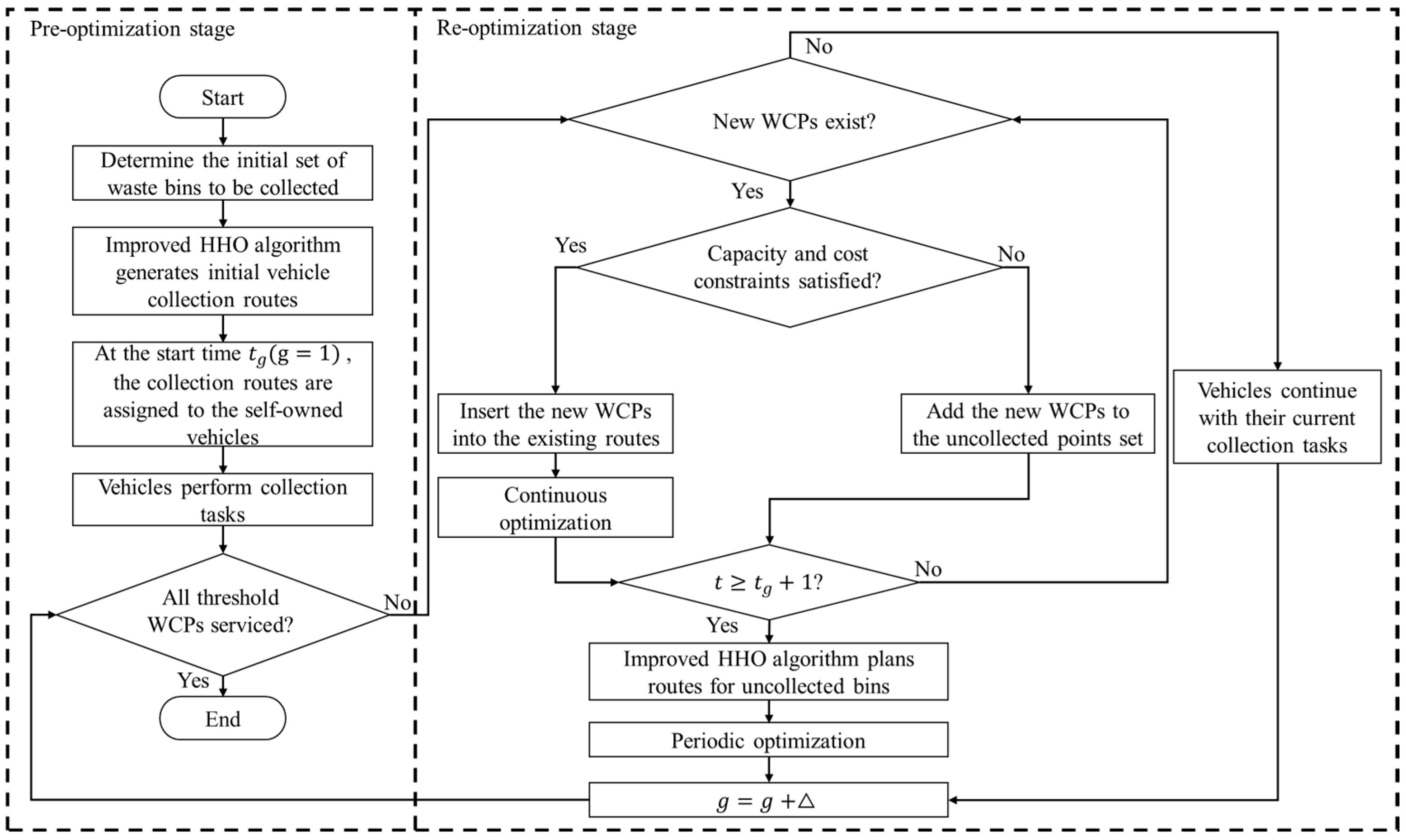
Considering the dynamic characteristics of the volume of waste in the re-optimization phase, existing research on optimization strategies mainly falls into two categories: periodic re-optimization and continuous re-optimization. The core issue of these strategies lies in when to update the path after the arrival of new information. Periodic re-optimization partitions the time horizon into fixed intervals and updates routes at the end of each interval, which may lead to delayed responses. Continuous re-optimization adjusts routes immediately upon receiving new demands, offering timely responses but requiring high real-time performance under frequent demand arrivals. To address the above issues, this study adopts a hybrid strategy that integrates periodic and continuous re-optimization. Continuous re-optimization means that when a dynamic demand arrives, the system immediately evaluates whether it satisfies both the capacity constraints and the cost constraints. If both are met, the demand is instantly inserted into the existing self-owned vehicle route, enabling a real-time response. Under periodic re-optimization, if a demand does not satisfy either of the above constraints, it is not processed immediately but is instead temporarily placed in a pending queue and will be uniformly handled by outsourced vehicles in the next decision period.

The detailed procedure of the algorithm for the waste collection scenario described above is as follows:

Step 1: Pre-optimization is performed at 9:00 and 21:00 by self-owned vehicles due to the bimodal distribution pattern.

Step 2: When a new waste collection point is added, it is necessary to check whether it satisfies the capacity constraint and the cost constraint of the self-owned vehicles.

Step 3: If Step 2 is satisfied, the system attempts to insert the waste collection point into each existing self-owned vehicle route and computes the associated cost increment [37]. Finally, the route with the minimum cost increment is selected as the optimal insertion route. If Step 2 is not satisfied, proceed to Step 4.

Step 4: The newly added WCP is allocated to the next period and serviced by outsourced vehicles, and the corresponding cost increment is calculated.

Step 5: Repeat Steps 2 to 4 until all WCPs have been serviced.

The flowchart of the algorithm is shown in Figure 2. Here, $t_g(g=0,1,2,\dots \dots m)$ represents the start time of period $g$.

5. Case Study

This section verifies the feasibility and effectiveness of the model and algorithm by introducing the relevant data for a case study and systematically comparing and analyzing the optimization results.

5.1. Data Sources

The model test data is derived from real-world data provided by a company in Zhuhai City, Guangdong Province. As a major provider of domestic waste collection information services, this company undertakes 90% of the waste collection work in Xiangzhou District. This area is primarily residential, and the waste generation characteristics and collection requirements are highly homogeneous across collection points. The specific vehicle parameters, algorithm parameters, and other relevant settings are listed in

Table 2. The values of the implemented parameters.

Parameter	Value	Unit
${\alpha }_1$	200	CNY/car
${\alpha }_2$	1	CNY/km
${\alpha }_3$	25	CNY/km
${\alpha }_{4,k=1}$	0.05	CNY/kg
${\alpha }_{4,k=2}$	0.03	CNY/kg
${\alpha }_{5,k=1}$	8	CNY/h
${\alpha }_{5,k=2}$	6	CNY/h
$Q_{n_1,k=1}$	2	ton
$Q_{n_1,k=2}$	3	ton
$Q_{n_2,k=1}$	1	ton
$Q_{n_2,k=2}$	2	ton
$v_n$	33	km/h
$t_d$	2	h
$f_o^{ser}$	30	min
$f_i^{ser}$	5	min
Initial escape energy	Random value within [−1, 1]	-
Number of iterations	100	-
Population size	100	-

. In particular, when $k=1$, the waste type is kitchen waste; when $k=2$, the waste type is other waste. In this study, the collection threshold for both kitchen waste and other waste was set at 0.8. In other words, a collection request is only generated when the accumulated waste in a bin reaches or exceeds 80% of its capacity.

This subsection details the statistical characteristics of the data used to validate the proposed model and algorithm. The WCPs are located within a subdistrict of Xiangzhou District, Zhuhai City, with the following geographic boundaries: longitude ranging from 113.42° E to 113.67° E and latitude ranging from 22.14° N to 22.32° N. This geographic range is also used for the subsequent random generation of dynamic demands, ensuring that newly generated demand points are located within the same region as the existing WCPs to maintain experimental consistency. Additionally, the coordinates of the key facilities are as follows: the kitchen waste transfer station is located at (113.558348, 22.222475), the other waste transfer station is at (113.555741, 22.235373), and the depot is at (113.547941, 22.22794).

Given the absence of waste generation datasets that align with the problem’s characteristics, the waste generation datasets were designed and generated based on the research requirements. In this case, a mixed model that integrates a bimodal Gaussian distribution and a uniform distribution was established to generate waste generation observation data. During the morning peak period (7:00–9:00), samples are drawn from $N_1$ (${\mu }_1$ = 123, ${\sigma }_1$ = 70); during the evening peak period (19:00–21:00), an equal number of samples are drawn from $N_2$ (${\mu }_2$ = 166, ${\sigma }_2$ = 48); and during the off-peak period (9:00–19:00), samples are generated from a uniform distribution.

5.2. Computational Results

Using the operational data, this study conducted the programming and simulation using MATLAB R2022b. The simulation was conducted on a computer (manufactured by Huawei Technologies Co., Ltd., Shenzhen, China) equipped with an Intel(R) Core (TM) i5-1240P 1.70 GHz processor, 16 GB RAM, and the 64-bit Windows 10 operating system.

5.2.1. Optimization Results Under Different Transport Capacity Configurations

To systematically assess the effectiveness of coordinated collection between self-owned and outsourced vehicles, three transport capacity configurations were established for comparison: ($A_1$) self-owned fleet only, ($A_2$) outsourced fleet only, and ($A_3$) a mixed fleet consisting of both. The total collection cost was adopted as the primary evaluation indicator to quantify the economic performance of each configuration. The specific results are presented in

Table 3. The results of different fleet configurations for different scales of WCPs.

Number of WCPs	${\mathit{A}}_{\mathbf{1}}$	${\mathit{A}}_{\mathbf{2}}$	${\mathit{A}}_{\mathbf{3}}$
	Total Collection Cost (CNY)
50	1309	1204	1324
100	1732	1920	1477
150	2614	2924	2210
200	3221	3409	2511
300	4276	4487	3298

.

Table 3 shows that the performance of different fleet configurations varies significantly across five instances of varying scales. In the small-scale scenario with 50 WCPs, Strategy $A_2$ achieves the optimal cost. However, the cost advantage of the mixed fleet $A_3$ becomes increasingly pronounced as the number of WCPs grows. When the number of WCPs reaches 100, the costs incurred by Strategies $A_1$ and $A_2$ are 17.2% and 30.0% higher than that of Strategy $A_3$, respectively. As the scale expands to 300 WCPs, this gap further widens to 29.7% and 36.1%, respectively. This indicates that although the use of a mixed fleets incurs slightly higher costs than a fully outsourced fleet at smaller scales, its cost-sharing effects gradually materialize as the scale expands, ultimately reducing overall collection costs. In summary, the mixed fleet $A_3$ effectively balances the flexibility of idle resources with the stability of self-owned vehicles, demonstrating significant economic advantages in large-scale collection tasks.

5.2.2. Optimization Results Under Different Re-Optimization Strategies

This study conducted simulation analysis under a mixed-fleet mode using three optimization strategies: periodic re-optimization ($B_1$), continuous re-optimization ($B_2$), and a hybrid strategy that integrates periodic and continuous re-optimization ($B_3$). The total collection cost was adopted as the primary evaluation indicator to quantify the economic performance of each strategy. The specific results are presented in

Table 4. The results of different optimization strategies for different scales of WCPs.

Number of WCPs	${\mathit{B}}_{\mathbf{1}}$	${\mathit{B}}_{\mathbf{2}}$	${\mathit{B}}_{\mathbf{3}}$
	Total Collection Cost (CNY)
50	1211	2204	1311
100	1498	3170	1482
150	1932	4503	2094
200	2300	6019	2359
300	3234	7456	3302

.

As shown in Table 4, among the experiments with different scales, the continuous re-optimization strategy $B_2$ consistently yields the highest collection cost. This is primarily attributed to its need to frequently respond to dynamic collection requests, which significantly increases the additional costs associated with route adjustments. In contrast, the periodic re-optimization strategy $B_1$ and the hybrid strategy $B_3$ exhibit relatively similar total costs, but the hybrid strategy $B_3$ possesses the capability to respond to dynamic demands in real time, enabling more flexible resource allocation during the collection process. This effectively reduces the risk of waste accumulation and environmental pollution.

5.2.3. Algorithm Comparison

The performance of the improved HHO algorithm was verified by comparing it with three algorithms: GA, SA, and the traditional HHO.

Table 5. Parameters for optimization algorithms.

Algorithm	Parameter	Value
GA	Population Size	100
	Maximum Iterations	100
	Crossover Rate	0.8
	Mutation Rate	0.01
SA	Initial Temperature	1000
	Final Temperature	10−8
	Cooling Coefficient	0.95
HHO	Population Size	100
	Maximum Iterations	100
	Initial Escape Energy	Random value within [−1, 1]

lists the parameter settings used for each algorithm, while

Table 6. The performance comparison of different algorithms.

	SA			GA			HHO			Improved HHO
No.	Cost (CNY) 1	Iterations 2	Time (min) 3	Cost (CNY)	Iterations	Time (min)	Cost (CNY)	Iterations	Time (min)	Cost (CNY)	Iterations	Time (min)
1	1630.54	66	6	1710.35	48	6	1680.81	56	7	1503.51	76	10
2	1625.92	68	7	1696.21	65	7	1677.21	66	8	1497.22	69	9
3	1598.77	70	7	1739.00	46	6	1689.14	69	8	1479.40	80	10
4	1570.00	72	7	1756.21	55	6	1665.20	55	6	1491.11	88	11
5	1621.31	50	6	1721.00	58	6	1678.21	49	6	1489.94	70	10
6	1600.28	57	6	1681.19	61	6	1667.98	57	6	1490.21	81	11
7	1610.91	71	6	1699.17	67	6	1698.21	51	6	1469.99	86	11
8	1588.80	70	6	1702.90	54	6	1691.11	52	6	1479.51	86	11
9	1622.00	58	6	1721.27	53	6	1680.65	55	6	1487.25	73	9
10	1610.21	59	6	1700.06	51	6	1688.22	61	7	1496.12	75	9

¹ Total collection cost (CNY). ² Number of iterations required for convergence. ³ Algorithm running time per run (minutes).

reports the solution results.

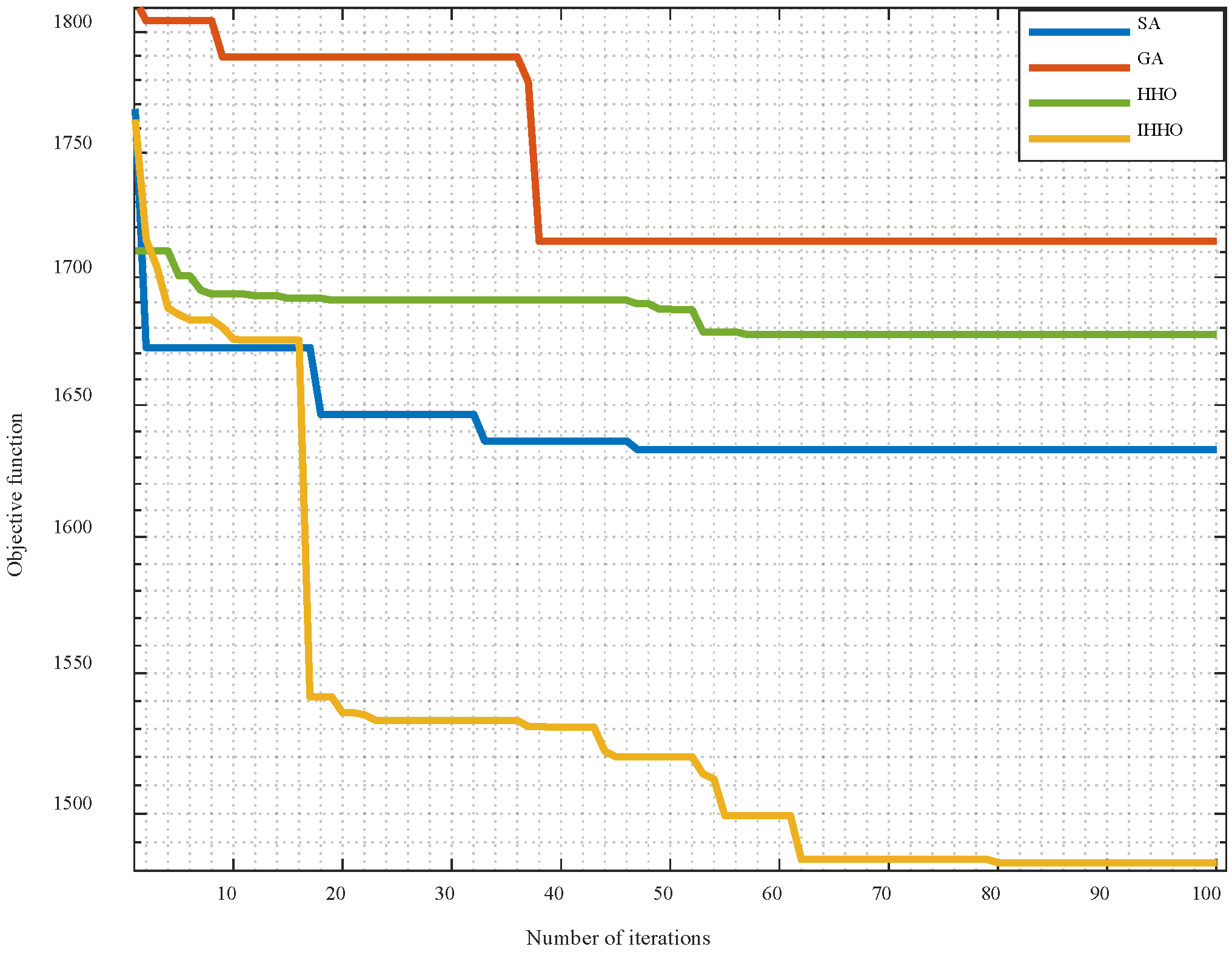
To ensure the accuracy of the experimental results, all optimization algorithms were executed under identical conditions to eliminate performance bias caused by external differences. Each algorithm was independently run 10 times based on 100 WCPs, and the detailed results are presented in Table 6. The convergence of each algorithm is illustrated in Figure 3.

As shown in Table 6, the optimal values achieved by SA, GA, the traditional HHO, and the improved HHO are 1570.00 CNY, 1681.19 CNY, 1665.20 CNY, and 1469.99 CNY, respectively, while the average values are 1611.874 CNY, 1712.736 CNY, 1681.674 CNY, and 1488.426 CNY, respectively. Although the improved HHO algorithm requires more iterations and a longer runtime than the other algorithms, it clearly achieves better solution quality, demonstrating its strong global search capability. This is also confirmed by Figure 3.

The preceding experiments have validated the superiority of the proposed improved HHO algorithm in convergence speed, computational efficiency, and stability. Next, we examined the algorithm’s applicability across different scales. Specifically, we constructed instances with 50, 100, and 300 WCPs to represent small, medium, and large operational scales, respectively. The detailed results are presented in

Table 7. Performance of the improved HHO algorithm for different scales of WCPS.

Number of WCPs	Improved HHO
	Total Collection Cost (CNY)	Number of Iterations	Running Time (min)
50	1316	76	3
100	1452	72	10
300	3220	87	18

.

As shown in Table 7, the improved HHO algorithm demonstrates good performance across different scales. As the number of WCPs increases from 50 to 300, the runtime increases from 3 min to 18 min. This near-linear growth trend demonstrates the good scalability of the algorithm. These results demonstrate that the improved HHO algorithm can effectively adapt to application scenarios with different operational scales and has practical engineering application value.

6. Sensitivity Analysis

This section further investigates the influence of key parameters on the model, specifically the time interval for periodic re-optimization and the collection threshold of the smart bins.

6.1. Time Interval in Periodic Re-Optimization

In the re-optimization phase, the time interval determines the frequency of route updates. Its setting largely influences the demand response time, thereby affecting the optimization results of the collection plan. This subsection details experiments conducted with different time intervals, with the total collection cost, variable cost, penalty cost, and runtime used as evaluation indicators.

As shown in

Table 8. The results using different time intervals.

Time Interval (min)	Total Collection Cost (CNY)	Fixed Cost (CNY)	Variable Cost (CNY)	Penalty Cost (CNY)	Running Time (min)
30	1328	600	383	345	18
60	1394	600	331	463	12
120	1491	600	218	673	10
240	1571	600	129	842	5
300	1724	600	123	1001	3

, different time interval settings have a significant impact on various cost components. Specifically, shorter time intervals lead to longer model runtimes. This is because a denser division of periods requires frequent route updates and adjustments, thereby significantly increasing the computational burden. Furthermore, as the time interval lengthens, the penalty cost caused by waste accumulation rises. In contrast, the variable operating cost of vehicles shows a decreasing trend, indicating that a longer time interval helps reduce additional transportation expenses incurred by frequent scheduling. Therefore, enterprises may set the update interval to between 60 and 120 min, which ensures a certain level of responsiveness while effectively controlling collection costs.

6.2. Collection Threshold of the Smart Bins

The acceptable accumulation time for kitchen waste differs significantly from that of other waste, primarily due to its distinct composition and physicochemical properties. Therefore, this subsection details experiments conducted with different collection threshold for different types of waste, with the total collection cost used as the evaluation indicator.

Table 9. The results using different collection thresholds for the different waste types.

		Collection Threshold for Kitchen Waste
		0.5	0.6	0.7	0.8	0.9
Collection threshold for other waste	0.5	2211	2145	2189	2113	2243
	0.6	2319	2119	2171	2114	2298
	0.7	2311	2178	2231	2229	2341
	0.8	2289	2190	2101	2321	2453
	0.9	2329	2267	2322	2381	2490

indicates that the collection cost is minimized when the collection thresholds for kitchen waste and other waste are set to 0.7 and 0.8, respectively. When both thresholds are set to 0.9, while the single-trip collection volume is maximized, the high risk of waste accumulation leads to an increase in total collection cost. Conversely, excessively low collection thresholds reduce the risk of waste accumulation but lead to higher vehicle scheduling costs and lower bin utilization. Therefore, considering both facility utilization efficiency and waste accumulation risk, setting the collection thresholds for kitchen waste and other waste to 0.7 and 0.8, respectively, can improve facility utilization while effectively controlling environmental risks and operational costs.

7. Conclusions and Future Works

This study investigated the dynamic routing optimization problem for multi-compartment vehicles in domestic waste collection under a mixed-fleet mode. A model was established with the objective of minimizing the collection costs of self-owned and outsourced vehicles, and a two-stage algorithm was designed to solve it. The proposed model and algorithm were empirically validated through experiments conducted under various scenarios. Finally, through sensitivity analysis of the key parameters, we derived several implications for management practice:

(1)

To balance timeliness and economy in waste collection, enterprises can set the time interval between 60 and 120 min. This range ensures a reasonable level of demand responsiveness while effectively controlling collection costs.

(2)

Excessively high clearance thresholds increase the risk of waste accumulation or even overflow. Conversely, excessively low thresholds reduce the risk of waste accumulation but lead to higher vehicle scheduling costs and lower bin utilization. Therefore, a balance must be struck between facility utilization efficiency and waste accumulation risk. Setting the clearance thresholds for kitchen waste and other waste within reasonable ranges can enhance facility utilization while effectively controlling environmental risks and operational costs.

This study makes several simplifying assumptions about real-world scenarios, including the omission of road turning restrictions, one-way streets, and traffic congestion, as well as the assumption of unlimited transfer station capacity. These simplifications deviate to some extent from actual scenarios. To address this limitation, we will introduce time-dependent travel time functions to capture traffic constraints in future studies. Meanwhile, waste transfer stations will be modeled as finite-capacity queuing systems, and the expected waiting time will be incorporated into the objective function to make the model more realistic. Furthermore, this study did not systematically validate other types of waste generation peak distributions. In the future, different peak distribution characteristics across various regions will be considered. Finally, while this study focused on minimizing total collection cost, it did not fully account for environmental impacts or employee workload balance. Future research will aim to construct a multi-dimensional optimization framework that encompasses social, economic, and environmental objectives. Specifically, the economic objective is to minimize the total collection cost, the social objective is to maximize workload balance, and the environmental objective is to minimize carbon emissions.

References

1. Kaza, S.; Yao, L.; Bhada-Tata, P.; Woerden, F. What a Waste 2.0: A Global Snapshot of Solid Waste Management to 2050; World Bank Publications: Washington, DC, USA, 2018. [Google Scholar] [CrossRef]
2. Ministry of Housing and Urban-Rural Development. 2024 Statistical Yearbook of Urban Construction. 2025. Available online: https://www.stats.gov.cn/sj/ndsj/ (accessed on 10 March 2026).
3. Hannan, M.A.; Akhtar, M.; Begum, R.A.; Basri, H.; Hussain, A.; Scavino, E. Capacitated vehicle-routing problem model for scheduled solid waste collection and route optimization using PSO algorithm. Waste Manag. 2018, 71, 31–41. [Google Scholar] [CrossRef]
4. Zhang, A.; Venkatesh, V.G.; Liu, Y.; Wan, M.; Qu, T.; Huisingh, D. Barriers to Smart Waste Management for a Circular Economy in China. J. Clean. Prod. 2019, 240, 118198. [Google Scholar] [CrossRef]
5. Bian, S.; Xue, Y.; Li, C.; Wu, W.; Ma, Z.; Okoro, J.O.; Harder, M.K. Depositing waste in ‘certain place’ at ‘certain time’: Does this policy improve recycling performance? Resour. Conserv. Recycl. 2022, 176, 105935. [Google Scholar] [CrossRef]
6. Anghinolfi, D.; Paolucci, M.; Robba, M.; Taramasso, A.C. A dynamic optimization model for solid waste recycling. Waste Manag. 2013, 33, 287–296. [Google Scholar] [CrossRef] [PubMed]
7. Abdallah, M.; Adghim, M.; Maraqa, M.; Aldahab, E. Simulation and optimization of dynamic waste collection routes. Waste Manag. Res. 2019, 37, 793–802. [Google Scholar] [CrossRef] [PubMed]
8. Exposito-Marquez, A.; Exposito-Izquierdo, C.; Brito-Santana, J.; Moreno-Pérez, J.A. Greedy randomized adaptive search procedure to design waste collection routes in La Palma. Comput. Ind. Eng. 2019, 137, 106047. [Google Scholar] [CrossRef]
9. Rahmanifar, G.; Mohammadi, M.; Sherafat, A.; Hajiaghaei-Keshteli, M.; Fusco, G.; Colombaroni, C. Heuristic approaches to address vehicle routing problem in the Iot-based waste management system. Expert Syst. Appl. 2023, 220, 119708. [Google Scholar] [CrossRef]
10. Hannan, M.A.; Marnun, A.A.; Hussain, A.; Basri, H.; Begum, R.A. A review on technologies and their usage in solid waste monitoring and management systems: Issues and challenges. Waste Manag. 2015, 43, 509–523. [Google Scholar] [CrossRef]
11. Akhtar, M.; Hannan, M.A.; Begum, R.A.; Basri, H.; Scavino, E. Backtracking search algorithm in CVRP models for efficient solid waste collection and route optimization. Waste Manag. 2017, 61, 117–128. [Google Scholar] [CrossRef]
12. Nowakowski, P.; Szwarc, K.; Boryczka, U. Combining an artificial intelligence algorithm and a novel vehicle for sustainable e-waste collection. Sci. Total Environ. 2020, 730, 138726. [Google Scholar] [CrossRef]
13. Idwan, S.; Mahmood, I.; Zubairi, J.A.; Matar, I. Optimal management of solid waste in smart cities using internet of things. Wirel. Pers. Commun. 2020, 110, 485–501. [Google Scholar] [CrossRef]
14. Jorge, D.; Antunes, A.P.; Ramos, T.R.P.; Barbosa-Póvoa, A.P. A hybrid metaheuristic for smart waste collection problems with workload concerns. Comput. Oper. Res. 2022, 137, 105518. [Google Scholar] [CrossRef]
15. de Morais, C.S.; Ramos, T.R.P.; Lopes, M.; Barbosa-Póvoa, A.P. A data-driven optimization approach to plan smart waste collection operations. Int. Trans. Oper. Res. 2024, 31, 2178–2208. [Google Scholar] [CrossRef]
16. Kim, J.; Manna, A.; Roy, A.; Moon, I. Clustered vehicle routing problem for waste collection with smart operational management approaches. Int. Trans. Oper. Res. 2025, 32, 863–887. [Google Scholar] [CrossRef]
17. Yang, J.; Tao, F.; Zhong, Y. Dynamic routing for waste collection and transportation with multi-compartment electric vehicle using smart waste bins. Waste Manag. Res. 2022, 40, 1199–1211. [Google Scholar] [CrossRef]
18. Mohammadi, M.; Rahmanifar, G.; Hajiaghaei-Keshteli, M.; Fusco, G.; Colombaroni, C.; Sherafat, A. A dynamic approach for the multi-compartment vehicle routing problem in waste management. Renew. Sustain. Energy Rev. 2023, 184, 113526. [Google Scholar] [CrossRef]
19. Markov, I.; Varone, S.; Bierlaire, M. Integrating a heterogeneous fixed fleet and a flexible assignment of destination depots in the waste collection VRP with intermediate facilities. Transp. Res. Part B-Methodol. 2016, 84, 256–273. [Google Scholar] [CrossRef]
20. Asefi, H.; Shahparvari, S.; Chhetri, P.; Lim, S. Variable fleet size and mix VRP with fleet heterogeneity in Integrated Solid Waste Management. J. Clean. Prod. 2019, 230, 1376–1395. [Google Scholar] [CrossRef]
21. Ghiani, G.; Manni, A.; Manni, E.; Moretto, V. Optimizing a waste collection system with solid waste transfer stations. Comput. Ind. Eng. 2021, 161, 107618. [Google Scholar] [CrossRef]
22. Cao, S.; Liao, W.; Huang, Y. Heterogeneous fleet recyclables collection routing optimization in a two-echelon collaborative reverse logistics network from circular economic and environmental perspective. Sci. Total Environ. 2021, 758, 144062. [Google Scholar] [CrossRef]
23. Wei, C.; Che, A.; Xue, L. A hierarchical integrated exact algorithm for multi-level capacitated arc routing problem in waste collection. Transp. Res. Part E Logist. Transp. Rev. 2025, 204, 104441. [Google Scholar] [CrossRef]
24. Nucamendi-Guillén, S.; Padilla, A.G.; Olivares-Benitez, E.; Moreno-Vega, M. The multi-depot open location routing problem with a heterogeneous fixed fleet. Expert Syst. Appl. 2021, 165, 113846. [Google Scholar] [CrossRef]
25. Xu, B.; Zhao, K.; Luo, Q.; Wu, G.; Pedrycz, W. A GV-drone arc routing approach for urban traffic patrol by coordinating a ground vehicle and multiple drones. Swarm Evol. Comput. 2023, 77, 101246. [Google Scholar] [CrossRef]
26. Lin, Z.; Xu, X.; Demir, E.; Laporte, G. Optimizing task assignment and routing operations with a heterogeneous fleet of unmanned aerial vehicles for emergency healthcare services. Comput. Oper. Res. 2025, 174, 106890. [Google Scholar] [CrossRef]
27. Heidari, A.A.; Mirjalili, S.; Faris, H.; Aljarah, I.; Mafarja, M.; Chen, H. Harris Hawks optimization: Algorithm and applications. Future Gener. Comput. Syst. 2019, 97, 849–872. [Google Scholar] [CrossRef]
28. Elgamal, Z.M.; Binti, N.; Tubishat, M.; Alswaitti, M.; Mirjalili, S. An improved harris Hawks optimization algorithm with simulated annealing for feature selection in the medical field. IEEE Access 2020, 8, 186638–186652. [Google Scholar] [CrossRef]
29. Cheng, F.; Liu, H. Charging strategies optimization for lithium-ion battery: Heterogeneous ensemble surrogate model-assisted advanced multi-objective optimization algorithm. Energy Convers. Manag. 2010, 342, 120170. [Google Scholar] [CrossRef]
30. Chen, X.; Qin, H.; Liu, S.; Chen, J.; Li, Y.; Zhu, X. Intelligent Scheduling Method for Cascade Reservoirs Driven by Dual Optimization of Harris Hawks and Marine Predators. Water 2025, 17, 3291. [Google Scholar] [CrossRef]
31. Gupta, S.; Deep, K.; Heidari, A.A.; Moayedi, H.; Wang, M. Opposition-based learning Harris hawks optimization with advanced transition rules: Principles and analysis. Expert Syst. Appl. 2020, 158, 113510. [Google Scholar] [CrossRef]
32. Nivethitha, V.; Aghila, G. Improved Harris Hawks optimization algorithm based data placement strategy for integrated cloud and edge computing. Intell. Autom. Soft Comput. 2023, 37, 887–904. [Google Scholar] [CrossRef]
33. Fahmy, H.; El-Gendy, E.M.; Mohamed, M.A.; Saafan, M. ECH3OA: An enhanced chimp-harris hawks optimization algorithm for copyright protection in Color images using watermarking techniques. Knowl.-Based Syst. 2023, 269, 110494. [Google Scholar] [CrossRef]
34. Bao, X.; Jia, H.; Lang, C. A novel hybrid harris Hawks optimization for color image multilevel thresholding segmentation. IEEE Access 2019, 7, 76529–76546. [Google Scholar] [CrossRef]
35. Sehgal, S.; Ganesh, A.; Malik, O.P. A memetic approach to multi-disciplinary design and numerical optimization problems using intensify slime mould optimizer. Appl. Intell. 2024, 54, 2031–2083. [Google Scholar] [CrossRef]
36. Sharma, H.; Bharali, J.; Motghare, M.; Arora, K.; Yoon, C.; Joshi, G.P. Development and evaluation of hybrid harris hawks optimization algorithms for advanced engineering applications. Sci. Rep. 2025, 15, 43123. [Google Scholar] [CrossRef] [PubMed]
37. Solomon, M.M. Algorithms for the vehicles routing and scheduling problem with time window constraints. Oper. Res. 1987, 35, 254–265. [Google Scholar] [CrossRef]
Figure 1. The dual-compartment vehicle collection process.
Systems 14 00461 g001
Figure 2. The flowchart of the proposed two-phase algorithm.
Systems 14 00461 g002
Figure 3. Convergence comparison of algorithms.
Systems 14 00461 g003