Pressure Wave Propagation Optimization Models for Supply Chain Risk Mitigation

Abstract

Supply chain (SC) disruption risk assessment and mitigation have attracted significant attention in both academia and practice. However, existing research predominantly focuses on unidirectional disruption propagation, either forward or backward, despite the reality that risks can propagate bi-directionally in complex supply chain networks. Furthermore, conventional assessment tools often concentrate on conceptualizing and quantifying risks, while risk mitigation requires mathematical optimization approaches. To bridge these gaps, this paper proposes a novel pressure wave-based approach inspired by fluid mechanics to assess bi-directional disruption propagation in cluster supply chain networks (CSCNs). The method conceptualizes disruptions as pressure signals that transmit between SC partners and explicitly quantifies disruption severity through wave intensity. By employing mathematical optimization, we develop a framework that assists managers in optimizing risk mitigation strategies, including inventory buffering and cross-chain cooperation. Numerical experiments demonstrate the effectiveness of the proposed method in explaining risk influencing factors, mitigating disruption risks, and achieving dynamic restructuring of SC structures. The results show that our approach reduces the Cluster Propagation Vulnerability Index (CPVI) by up to 40% compared to baseline models without optimization decisions.

1. Introduction

In recent years, a growing number of products, such as lithium batteries, rely on raw materials sourced from various countries and are supported by intricately interconnected supply chains (SCs). This has led to continuously evolving risks throughout the entire lifecycle of SC segments, particularly disruption risks [1]. In academia, substantial research has been devoted to studying disruption risks within general SC structures. The propagation of such risks from upstream to downstream is referred to as the ripple effect [2,3].

As global connections and integrations deepen, interdependent supply chain networks (SCNs) and intertwined SCs from industry clusters tend to form vast large-scale networks, called cluster SCNs (CSCNs) [4,5,6]. In such large-scale SCNs, substantial cooperation and competition among partners at the same tier coexist. This suggests that, in reality, SC disruption risks can propagate bi-directionally, yet this phenomenon has not garnered sufficient attention in academic research. As CSCNs are critical in regional and international trades, SC disruptions in such complex networks have received great attention from the SC risk management community, and it is urgent to mitigate bi-directional disruption risks in such complex structures [5,7].

The existing literature exhibits significant limitations in analyzing the propagation nature of SC disruptions: (i) Most studies have overlooked the impact of cooperation and competition among partners at the same tier on risk propagation [7]. In practice, competition and cooperation between nodes at the same tier are common in CSCNs, which influence the intensity and propagation path of SC disruptions [8,9]. (ii) Existing research primarily focuses on forward SC disruption propagation, while in reality, SC disruptions can propagate simultaneously in both directions with the flow information [4,9,10]. (iii) Existing studies often consider only risk assessment or risk mitigation strategies separately, without combining them. Methods such as stochastic programming and robust optimization focus on handling uncertain parameters rather than the propagation mechanism of SC disruption risks. Therefore, this work first proposes a model that can describe the mechanism of bi-directional disruption propagation. Furthermore, by considering managerial decisions, it incorporates risk mitigation strategies into risk assessments and uses mathematical programming for optimization.

To address these methodological gaps, inspired by pressure wave theory in fluid mechanics, we first propose a novel approach to assess bi-directional disruption propagation. This method employs analogical reasoning that facilitates the transfer of information from well-understood domains to novel contexts and focuses on similarities between the source domain and the target domain [11]. In fluid mechanics, pressure wave theory explains how pressure caused by a perturbation propagates in a certain medium. The flow of resources and information in an SCN is like the flow of a fluid through a pipe, which is a common metaphor in academia [12]. Drawing an analogy from physical concepts in pressure waves to the tunable parameters of the SC domain, we systematically examine how these parameters influence the propagation path and intensity of disruptions.

Building on this analogy, we propose an interpretable mathematical framework for disruption mitigation. When evaluating the risk of individual members, risk mitigation strategies can be informed by the stress wave model. Importantly, this framework utilizes the principles of transmitted and reflected waves to quantify both forward and backward propagation of SC disruptions simultaneously. We introduce two evaluation metrics—the Sub-network Propagation Vulnerability Index (SPVI) and the Cluster Propagation Vulnerability Index (CPVI)—to assess risks at the level of individual SCs and clustered SC networks, respectively. Particularly, we incorporate a series of risk mitigation decisions into the physical parameters, thereby constructing the pressure wave model as a mathematical programming model to ultimately achieve decision optimization. This work establishes a novel analogy between pressure wave dynamics and SC disruption propagation, providing an intuitive and physically-grounded explanation for the complex phenomenon of bi-directional risk flow. In addition, it combines risk quantification models with mathematical optimization to guide managerial decision-making.

The remainder of this paper is organized as follows. Section 2 presents the related literature. Section 3 states the studied problem. In Section 4, we establish a conceptual model to analogize pressure waves with SC disruptions. Section 5 and Section 6 provide mathematical frameworks to solve the proposed problem. Section 7 provides managerial insights through a series of case studies. Section 8 concludes with important results and outlines future research.

2. Literature Review

A substantial body of research has sought to understand and mitigate the impacts of SC disruptions. This review synthesizes the literature into three key streams: (1) studies on disruption propagation mechanisms, particularly the ripple effect; (2) quantitative methods for disruption assessment; and (3) the application of analogical reasoning in SC risk management. By critically examining the limitations of prior work, this section will clarify the significant research gaps that our study aims to address.

2.1. SC Risk Assessment and Disruption Propagation

Assessing how disruption risks propagate across SC networks (SCNs) has become a central issue in SC risk management. Among various perspectives, the ripple effect has been widely used to characterize how disruptions initiated at one node propagate to other connected partners [2]. Subsequent studies have employed mathematical programming and simulation to evaluate the impacts of ripple effects on performance indicators such as service level, production capacity, and transportation cost [13,14,15,16]. These models are effective in measuring aggregate losses and performance degradation under given disruption scenarios. However, they typically treat disruption propagation as an outcome of discrete structural connections rather than as a process governed by quantifiable transmission mechanisms.

A major limitation of existing ripple-effect models lies in their inability to explicitly quantify how different factors influence the strength, speed, and attenuation of disruption propagation. Most studies implicitly assume that disruptions are transmitted through fixed links, without modeling how variables such as inventory buffers, order allocation, production feedback, or network density modulate propagation intensity. Although several works have introduced continuous-state representations into SC analysis, their focus has largely remained on production and inventory dynamics rather than on disruption transmission mechanisms. Existing uncertainty-aware optimization models, including stochastic and robust programming, primarily focus on ex-ante representations of uncertainty through probabilistic distributions or membership functions. These approaches implicitly assume that uncertainty affects decision variables directly but do not explicitly model how risk propagates, accumulates, and attenuates across supply chain structures. For example, refs. [17,18] employ system dynamics and hybrid simulation to study operational interactions, while refs. [19,20] analyze how continuous inventory review and control policies influence recovery performance. Yet these models do not explicitly describe how disruption pressure propagates through the network.

An even more fundamental gap concerns the treatment of disruption directionality. The vast majority of ripple-effect studies model propagation as unidirectional, from upstream suppliers to downstream customers. However, empirical evidence shows that downstream disturbances such as demand collapses, order cancellations, and financial stress can propagate backward and significantly affect upstream partners. Ref. [10] demonstrates that losses experienced by downstream firms after the Great East Japan Earthquake influenced upstream production decisions. Several studies have attempted to relate ripple effects to the bullwhip effect [21,22], yet they do not explicitly formalize the feedback loops between forward and backward propagation. Agent-based approaches such as [9] simulate bi-directional ripple effects, but lack a rigorous mathematical structure to quantify the coupling between forward and backward transmission. As a result, current risk assessment models remain limited in their ability to capture how disruption pressures are amplified, reflected, and redistributed across interconnected SCs.

2.2. Mathematical Optimization for Risk Mitigation

In parallel with risk assessment, a large body of literature has developed mathematical optimization models to design disruption mitigation strategies. These models typically focus on decisions such as inventory allocation, production reconfiguration, supplier selection, and transportation planning in order to minimize cost, maximize service level, or enhance SC resilience under disruption [13,14,15,16]. In most cases, however, disruption impacts are either imposed exogenously or summarized through scenario-based parameters, while the propagation of risk itself is not endogenously modeled.

This leads to a structural separation between risk assessment and risk mitigation in the existing literature. On the one hand, Bayesian networks, simulation, and network-based approaches are used to evaluate disruption risks [23,24,25,26,27]. To simplify the hierarchical tree structure while preserving key information of risk source, they develop an entropy-based optimization model. The Bayesian network is a probabilistic graphical model, which uses the directed acyclic graph (DAG) to integrate probabilistic information on state transfers. This technical limitation of DAG makes it hard for BNs to consider bi-directional SC disruption propagation. The arcs in the DAG characterize the propagation path of the disruptions and the state transfers of nodes in the DAG characterize the evolution of disruptions under ripple effects. Ref. [28] utilizes Bayesian networks to quantify supplier disruptions under ripple effects and develop a bi-objective stochastic programming model to optimize supplier selection decisions. Ref. [23] develops the BN framework for modeling ripple effect and propose a metric to quantify the ripple effect of supplier disruption on the manufacturer in terms of total expected utility and service level. To assess ripple effect in the presence of disturbed probabilistic information, ref. [24] utilizes the causal Bayesian network and the do-calculus method. BNs assume that the states of SC partners can be represented by a series of pre-defined discrete states, which lack realistic interpretability and are difficult to be fully defined [29]. Ref. [30] employs Bayesian network theory to quantify the cascading ripple effect of SC risk propagation, utilizing developed risk exposure and resilience indices to assess node vulnerability and adaptability, thereby providing a holistic measurement approach for enhanced risk management. Ref. [31] conceptualizes SC resilience through a systems theory and cybernetics lens, defining it as the dynamic balance between vulnerability and recoverability. On the other hand, optimization models are employed to design mitigation strategies based on pre-estimated risk measures. The lack of an integrated framework means that mitigation decisions cannot directly reshape the underlying disruption propagation process, but only react to its outcomes.

Only a limited number of studies have attempted to integrate disruption propagation and mitigation decisions within a single modeling framework. For example, ref. [15] embeds ripple effects into a robust optimization model for reverse SCs, while ref. [16] formulate a multi-objective mixed-integer program that simultaneously evaluates dynamic ripple risks and logistics decisions. Ref. [14] also integrates network reconfiguration with disruption dynamics to assess viability. Despite these advances, even these integrated models treat ripple effects largely as scenario-dependent disturbances rather than as endogenous dynamic processes that respond to managerial interventions. Consequently, existing optimization approaches remain limited in their ability to design policies that actively control how disruption risks propagate across interconnected SC networks.

2.3. Analogies Applied to SC Risk Management

Analogical reasoning, the process of transferring knowledge from one domain to another, has gained increasing attention in recent SC risk research. Drawing on foundational work in metaphorical transfer methodology, ref. [32] proposes a metaphorical transfer pathway framework to support the development of novel SC theories. Similarly, ref. [33] analogizes the four fundamental forces of physics—internal, external, collaborative, and gravitational—as factors influencing SC key performance indicators. In the area of risk management, ref. [34] compares the immune system to SC risk management, proposing a multi-layered framework that offers both short- and long-term protection against diverse risks. Further extending biological analogies, ref. [35] draws inspiration from trophic chain dynamics, modeling predator–prey interactions to conceptualize viable SCs. More recently, ref. [36] aligns innate and adaptive immunity with proactive and reactive SC resilience strategies, introducing a set of immune-inspired mechanisms for building resilient SCs. Despite these advances, no studies to date have explored the application of fluid mechanics to SC risk assessment. In fluid mechanics, pressure wave theory explains how perturbations propagate through a medium. This theory has been practically applied in fields such as structural health monitoring, where pressure wave propagation is used to detect anomalies in pipelines and ducts [37].

2.4. Summary

In summary, prior research has advanced our understanding of SC disruptions by examining their propagation mechanisms, developing quantitative assessment tools, and drawing on cross-disciplinary analogies. However, most studies either model risks as discrete states or assume unidirectional propagation, which fails to capture the continuous evolution of disruption intensity and the bi-directional feedback observed in real supply networks. To address these gaps, our work develops a novel framework inspired by pressure wave theory that treats risks as continuous variables and models disruption propagation as a two-way dynamic process, thereby providing a more realistic basis for SC risk assessment. This study positions itself at the intersection of disruption propagation modeling and analytical dynamics by introducing a pressure wave-inspired framework for clustered supply networks. Unlike conventional ripple-effect or diffusion-based approaches, disruption pressure is modeled as a continuous state variable whose evolution follows a structured propagation mechanism with damping, historical accumulation, and boundary feedback. This enables a unified representation of temporal continuity, spatial structure, and subnetwork heterogeneity within a single analytical framework. The proposed pressure wave-based model conceptualizes uncertainty as a dynamic disturbance that propagates through SC following a structured transmission law. Moreover, by abstracting sourcing flexibility and mitigation capacity into effective structural parameters rather than explicit combinatorial decisions, the proposed model isolates the fundamental transmission properties of clustered supply chains under stress. It complements existing optimization- and simulation-based approaches by providing a benchmark dynamic characterization of disruption propagation, which can serve as a foundation for subsequent extensions that explicitly incorporate capacity constraints, nonlinear interactions, and strategic decision variables.

Table 1. Comparison of related studies and our work.

Study	Problem Setting						Assessment Tool
			SC Disruption
	System Modeling		Propagation Direction
	Continuous	Discrete	Forward	Backward	Explainable Mechanism	Tunable Parameter
[2]	✓		✓				Opt. Con.
[30]		✓	✓				BN
[21]		✓	✓				Simulation
[31]		✓	✓				BN
[10]		✓		✓	✓		Simulation
[24]		✓	✓				BN
[4]		✓	✓				Simulation
[3]		✓	✓	✓			Net. Ana.
[9]		✓	✓	✓			Simulation
This paper	✓		✓	✓	✓	✓	Pressure wave analogy

Opt. Con.: Optimal control; Net. Ana.: Network analysis.

summarizes the main differences between related existing studies and our work.

3. Problem Statement

This study aims to effectively assess bi-directional supply chain (SC) disruptions and to support managerial decision-making in mitigating such risks through optimization. We seek to explore how specific tunable parameters influence the intensity and propagation pathways of SC disruptions. As global interconnections deepen, star-shaped SC structures have become increasingly prevalent, characterized by focal firms at the center surrounded by interdependent partners. These partners interact via logistics, financial, and information flows, forming a networked structure known as a cluster supply chain network (CSCN) [4].

In a typical CSCN, partners are distributed across different geographic clusters and belong to interrelated industries. Partners within the same region or industry often constitute a single-chain structure, corresponding to a conventional SC network. A CSCN generally comprises multiple such single-chain sub-networks and evolves dynamically with order cycles. Collaboration occurs not only within each single chain but also across different chains within the CSCN.

We contend that the proposed method is applicable to multi-echelon SCs, as they can be decomposed into a series of two-echelon structures. Therefore, for the sake of conciseness, this study employs a simplified two-echelon CSCN to model the problem under investigation. To characterize such a CSCN, we consider a network composed of several interdependent single SCs, where supply relationships dictate the paths of disruption propagation. Suppliers and manufacturers are treated as sources of forward and backward propagation, respectively. The evaluation extends beyond individual partners to encompass sub-networks and the CSCN as a whole. These issues are examined under the following scenario: a CSCN subjected to simultaneous forward and backward disruptions.

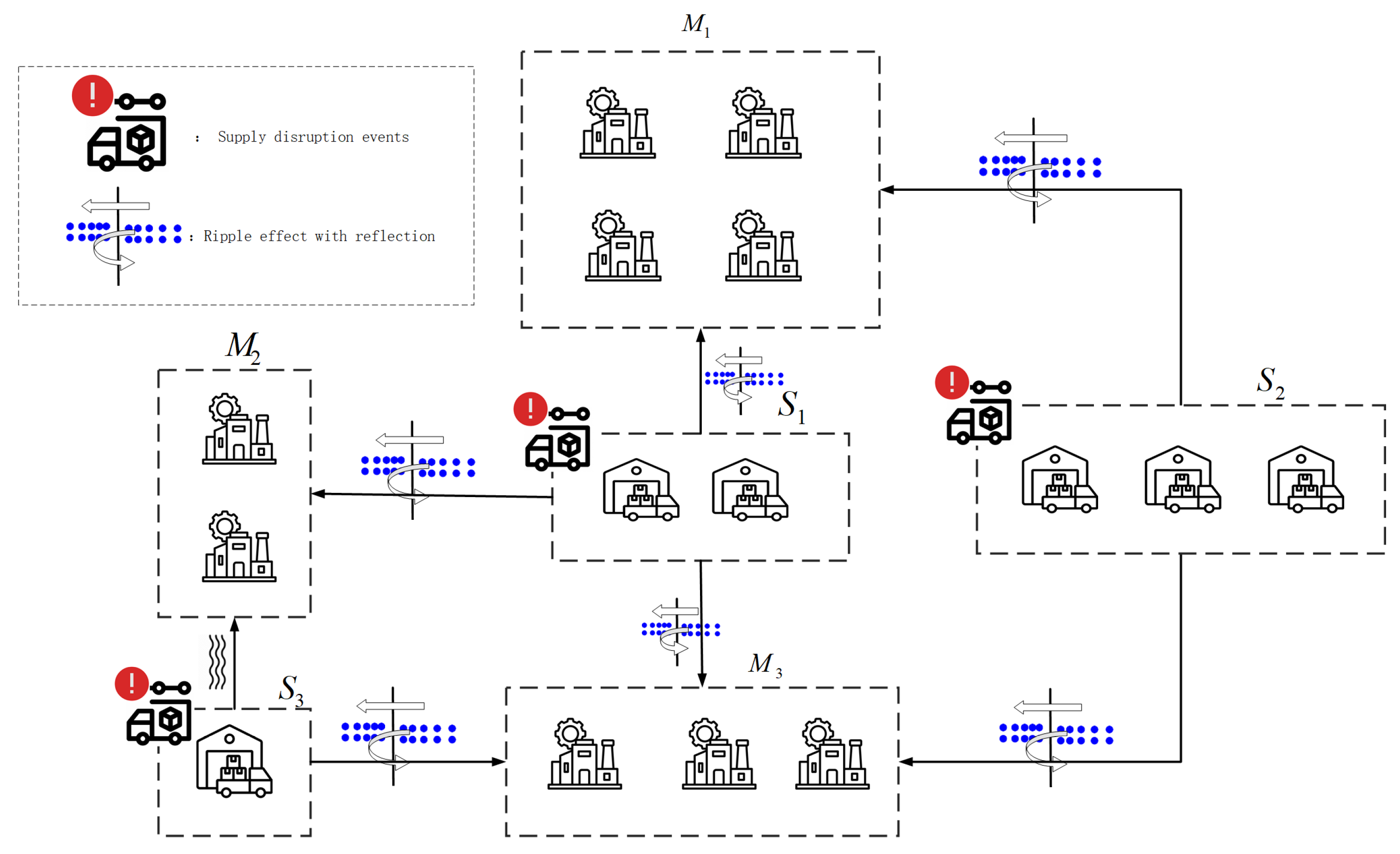
The structure of the studied CSCN is first introduced. It consists of multiple sub-networks (i.e., individual SCs) containing manufacturer and supplier sets from several related yet distinct industries. Each supplier set belongs to multiple sub-networks. Given the geographic clustering of manufacturers, each manufacturer set is assigned to only one sub-network. The set of these two-echelon sub-networks is denoted by $\mathcal{N}={\mathcal{N}}_1,\cdots ,{\mathcal{N}}_K$. Within a sub-network $\mathcal{N}k\in \mathcal{N}$, the manufacturer sets are denoted by $\mathcal{M}k=mk1,\cdots ,mk{X}_k$. The supplier sets are denoted by $\mathcal{S}=\mathcal{S}1,\cdots ,\mathcal{S}L$. For a supplier set $\mathcal{S}l\in \mathcal{S}$, the individual suppliers are denoted by $S_l=sl{y}_1,\cdots ,sl{y}_l$. Thus, there are $y_l$ suppliers in supplier set $S_l$. An assumption is made that suppliers within the same set offer interchangeable raw materials, while different supplier sets provide distinct materials. A manufacturer can purchase raw materials and determine purchasing quantities from all suppliers within its sub-network. Consequently, an auxiliary variable $R({\mathcal{N}}_k,{\mathcal{S}}_l)=\{0,1\}$ is introduced to denote whether supplier set ${\mathcal{S}}_l$ offers materials to sub-network ${\mathcal{N}}_k$. A key feature of CSCNs is cross-chain competition and cooperation. Specifically, if two manufacturer sets both possess all the raw materials required to produce a particular product, then the manufacturers across these sets can engage in cross-chain cooperation. Simultaneously, this implies that a competitive purchasing relationship exists between them.

For example, Figure 1 depicts the structure of the studied CSCN. There are three sub-networks, ${\mathcal{N}}_1$, ${\mathcal{N}}_2$ and ${\mathcal{N}}_3$. Thus, we have $M_1=\{m_{11},m_{12},m_{13},m_{14}\}$, $M_2=\{m_{21},m_{22}\}$, $M_3=\{m_{11},m_{12},m_{13}\}$, $S_1=\{s_{11},s_{12}\}$, $S_2=\{s_{21},s_{22},s_{23}\}$ and $S_3=\left\{s_{31}\right\}$. The supplier set $S_1$ offers raw materials for all sub-networks, supplier set $S_2$ offers raw materials for the sub-network ${\mathcal{N}}_1$ and the sub-network ${\mathcal{N}}_3$, and the supplier set $S_3$ offers raw materials for the sub-network ${\mathcal{N}}_2$ and the sub-network ${\mathcal{N}}_3$. Thus, we have $R({\mathcal{N}}_1,{\mathcal{S}}_1)=R({\mathcal{N}}_2,{\mathcal{S}}_1)=R({\mathcal{N}}_3,{\mathcal{S}}_1)=R({\mathcal{N}}_1,{\mathcal{S}}_2)=R({\mathcal{N}}_3,{\mathcal{S}}_2)=R({\mathcal{N}}_2,{\mathcal{S}}_3)=R({\mathcal{N}}_3,{\mathcal{S}}_3)=1$ and $R({\mathcal{N}}_2,{\mathcal{S}}_2)=R({\mathcal{N}}_1,{\mathcal{S}}_3)=0$.

Let us consider a multi-period disruption risk propagation problem. First, it is assumed that the number of raw material types required by each manufacturer equals the number of supply sets in the sub-network to which it belongs. For example, manufacturer $m_{11}$ in Figure 1 requires two types of raw materials provided by supply sets $S_1$ and $S_2$. In line with multiple sourcing strategies for risk mitigation, each manufacturer may allocate purchase orders across several suppliers.

In the literature, disruption events and risks are often referred to as stress testing for supply chains [39]. Thus, disruption risks can be analogized as pressure, and disruption events as pressure perturbations. Suppliers, as the first layer of the CSCN, are the initial points affected by external pressure perturbations. On the one hand, pressure perturbations at a given supplier propagate to all manufacturers within the sub-network it supplies, making suppliers the sources of forward disruption propagation. On the other hand, due to constraints imposed by orders and contracts, a manufacturer may feed back part of its pressure to its suppliers. Backward propagation of supply chain disruptions refers to the upstream transmission of disruption pressure from downstream partners to their suppliers. While disruptions originate upstream and cascade downstream through material flows, backward propagation is triggered when downstream partners respond to shortages, delays, or quality issues by intensifying demand, expediting orders, or imposing contractual penalties. These responses generate additional operational stress on suppliers, potentially amplifying existing disruptions or inducing new upstream failures. Although such backward propagation does not rely on physical logistics, it can be transmitted through information flows. Consequently, manufacturers act as pressure sources for backward disruption propagation.

To cope with these risks, manufacturers can establish risk mitigation inventory to absorb part of the forward pressure [9]. Each manufacturer must decide from which suppliers to procure raw materials and in what quantities. If the raw materials required by one sub-network include all materials needed by another sub-network, the latter may transfer its orders to the former through cross-chain collaboration—though at a substantially higher cost. This necessitates that manufacturers determine how much of their orders to allocate to other manufacturers. Additionally, manufacturers may hold risk mitigation inventory to reduce stockout penalties arising from unmet customer demand. In the proposed model, the quantities of raw materials purchased by manufacturers are treated as decision variables. Accordingly, suppliers are assumed to have effectively unlimited supply capacity. This assumption does not imply that individual suppliers possess infinite physical capacity. Rather, it reflects a managerial setting in which manufacturers can maintain effective supply availability by reallocating orders, diversifying sourcing, or introducing additional suppliers (e.g., backup suppliers) when necessary. As a result, potential capacity limitations for individual suppliers are externalized from the propagation dynamics and embedded implicitly in upstream structural adjustment decisions, which are beyond the scope of the present study.

The studied problem is based on the following assumptions:

(1)

The suppliers have sufficient supply capacity;

(2)

Suppliers in the same supplier set provide substitute raw materials;

(3)

Perturbations from the external and backward SC disruptions to suppliers are linearly superimposed;

(4)

According to assumption (3), do not consider external perturbations on the manufacturers, which does not affect subsequent studies;

(5)

The quantity of raw materials purchased by manufacturers must meet their needs;

(6)

The cost of risk mitigation inventory is linearly proportional to its quantity.

4. Modeling the SC Disruption via Pressure Wave Theory

This section develops a mathematical model for the SC disruption propagation by analogy with pressure wave theory in fluid mechanics. This novel analogy provides a dynamic and bi-directional view of risk propagation, emphasizing how disruptions not only flow downstream but also reflect upstream through contractual and operational feedback. Key conceptual correspondences are summarized in the parameter list in Section 6.

4.1. Foundations of Pressure Wave Theory

In fluid mechanics, a local pressure perturbation in a compressible medium propagates as a longitudinal pressure (acoustic) wave. Its spatiotemporal evolution is governed by the classic wave equation:

$${\displaystyle \frac{{\partial }^{2}p}{\partial t^2}}=c^2{\displaystyle \frac{{\partial }^{2}p}{\partial x^2}},$$

(1)

where $p=p(x,t)$ is the pressure at position x and time t, and c is the speed of sound in the medium. To account for energy dissipation during propagation (e.g., due to viscosity), a damping term is introduced:

$${\displaystyle \frac{{\partial }^{2}p}{\partial t^2}}+2\alpha {\displaystyle \frac{\partial p}{\partial t}}=c^2{\displaystyle \frac{{\partial }^{2}p}{\partial x^2}},$$

(2)

where $\alpha$ is the damping coefficient, leading to an exponential decay of the wave amplitude: $A\left(t\right)\propto e^{-\alpha t}$. The solution to this second-order equation depends on both current conditions and historical perturbations, embodying a historical cumulative effect.

A critical phenomenon occurs when a wave encounters an interface between two media with different acoustic impedances $z=\rho c$, where $\rho$ is mass density. The impedance z quantifies the medium’s resistance to pressure perturbations. At the interface, the incident wave $p^{\mathrm{inc}}\left(t\right)$ splits into a reflected wave $p^{\mathrm{ref}}\left(t\right)$ and a transmitted wave $p^{\mathrm{tra}}\left(t\right)$. The pressure must be continuous across the interface, yielding the boundary condition:

$$p^{\mathrm{tra}}\left(t\right)=p^{\mathrm{inc}}\left(t\right)+p^{\mathrm{ref}}\left(t\right).$$

(3)

The proportions of reflected and transmitted energy are governed by the reflection and transmission coefficients:

$$\begin{array}{cc}\hfill R& ={\displaystyle \frac{z_2-z_1}{z_1+z_2}},\hfill \end{array}$$

(4)

$$T=1+R={\displaystyle \frac{2z_2}{z_1+z_2}}.$$

(5)

Consequently, the waves are given by:

$$p^{\mathrm{ref}}\left(t\right)=R·p^{\mathrm{inc}}\left(t\right),$$

(6)

$$p^{\mathrm{tra}}\left(t\right)=T·p^{\mathrm{inc}}\left(t\right).$$

(7)

This framework perfectly models bi-directional energy flow: the source medium is affected by both the original perturbation and the reflected wave, while the receiving medium is driven by the transmitted wave.

4.2. Analogizing Forward SC Disruption Propagation to a Single Medium

We first model the downstream ripple effect within a single Cluster Supply Chain Network (CSCN) sub-network using the single-medium wave framework (Equation (2)). A CSCN comprises several such medium-like sub-networks, each representing a cluster of partners connected by material, information, and financial flows.

• Pressure $\mathit{p}(\mathit{x},\mathit{t})$: Analogous to the real-time risk exposure or operational stress level at a specific SC node (e.g., a manufacturer). It quantifies the severity of disruptions such as material shortages or logistics delays. A higher p indicates greater performance degradation.
• Position $\mathit{x}$: This is not mere physical distance. It is analogized to a generalized, multi-dimensional partnership distance, integrating factors like relational proximity, contractual tightness, information-sharing efficiency, and logistical lead time [12,40]. It defines the topology for risk propagation.
• Speed of sound $\mathit{c}$: Analogous to the velocity of disruption propagation within the sub-network. It depends on the efficiency of information flow and the agility of partner response mechanisms. Faster information sharing (high c) allows quicker detection and reaction, potentially dampening the wave’s peak amplitude.
• Damping coefficient $\mathit{\alpha }$: Analogous to the intrinsic, passive resilience of a node or the sub-network. This encompasses capacities like strategic safety stock, redundancy in processes, and financial buffers. These factors absorb disruption energy, converting it into manageable costs rather than cascading failures, leading to an exponential decay in disruption intensity over time [41,42]. The term $2\alpha {\displaystyle \frac{\partial p}{\partial t}}$ in Equation (2) models this mitigation effect.
• Mass density $\mathit{\rho }$ and Acoustic impedance $\mathit{z}=\mathit{\rho }\mathit{c}$: The density $\rho$ is analogized to SC network density—the number and closeness of connections within a partner set (e.g., a supplier set). A denser network ($\rho \uparrow$) typically offers more alternative pathways, increasing its intrinsic resistance to disruption, thus raising z. Acoustic impedance z, therefore, represents the overall resilience impedance of a sub-network. A high z implies a strong inherent ability to block or absorb disruption pressures.
• Historical cumulative effect: The wave equation’s dependence on initial conditions mirrors the disruption tail in SCs [43,44]. Past disruptions (historical perturbations) leave a residual stress on the system, affecting its susceptibility to new events and its recovery trajectory.

An exogenous disruption (e.g., a supplier factory fire) acts as the initial pressure perturbation $p_0$. This perturbation propagates downstream through the network topology defined by x, its temporal evolution shaped by the network’s propagation speed c and attenuated by its collective damping $\alpha$. In research, supply chain disruptions and risks can be seen as quantifiable states, corresponding to the loss of supply capacity or production capacity of supply chain members. In research, SC disruptions and risks can be viewed as quantifiable states, corresponding to the loss of supply capability or production capacity of SC members [2,45]. This paper uses stress waves to similarly handle this loss of capacity.

We can examine forward propagation of SC disruptions in a CSCN through the lens of pressure wave theory. To begin, it is reasonable to conceptualize SC risk propagation as a form of longitudinal wave, given that risk inherently propagates along the structure of the SC. Perturbations that generate pressure can be likened to supply disruptions experienced by upstream suppliers. These disturbances originate from a specific node and transmit through the network, modulated by factors such as the strength of inter-firm partnerships, the resilience of individual partners, and the structural configuration of the supply chain. As multiple sources of pressure converge, their effects can propagate downstream, ultimately impacting manufacturers. This analogy implies that mathematical models originally developed to describe wave phenomena could be effectively repurposed to simulate and analyze the diffusion of disruptions across SCs. A notable advantage of this tool is that researchers or managers can study how factors of interest affect the propagation of disruptions within this framework. Moreover, even if the parameters of interest are uncertain, methods such as stochastic programming can further be incorporated into the stress wave model. For example, this paper considers simple random factors such as exogenous disturbances and demand, and demonstrates how they influence risk evolution.

4.3. Modeling Bi-Directional Propagation Based on Reflected and Transmitted Wave

The novel contribution of this work lies in applying the two-medium wave interaction model to bi-directional SC risk propagation. This formally captures how disruption pressures not only transmit downstream but also reflect upstream due to contractual feedback loops.

Consider the interface between two CSCN sub-networks: an upstream Supplier Set (Medium 1) and a downstream Manufacturer Set (Medium 2). Their interaction is governed by contracts and information flows.

• Impedance Mismatch (${\mathit{z}}_{\mathbf{1}}\ne {\mathit{z}}_{\mathbf{2}}$): This is the driver of reflection. Different sub-networks have different resilience characteristics. For instance:

  –

  A supplier set with high impedance ${\mathit{z}}_{\mathbf{1}}$ might result from a multi-sourcing strategy (high density ${\rho }_1$) and strong collective bargaining power (slow, negotiated response, implying lower $c_1$). It is resistant to absorbing disruptions.

  –

  A manufacturer set with low impedance ${\mathit{z}}_{\mathbf{2}}$ might result from single sourcing (low ${\rho }_2$) and just-in-time processes requiring rapid response (high $c_2$). It is vulnerable and less resistant.

  This mismatch determines the coefficients R and T via Equations (4) and (5).
• Incident wave ${\mathit{p}}^{\mathbf{inc}}\left(\mathit{t}\right)$: Represents the disruption pressure arriving at the interface from the upstream supplier set (e.g., a declared capacity reduction).
• Transmitted wave ${\mathit{p}}^{\mathbf{tra}}\left(\mathit{t}\right)=\mathit{T}·{\mathit{p}}^{\mathbf{inc}}$: This is the portion of the original disruption that successfully propagates downstream to affect the manufacturers. It models the classical forward ripple effect. If T is large (e.g., when $z_2\gg z_1$), most of the pressure passes through, severely impacting manufacturers.
• Reflected wave ${\mathit{p}}^{\mathbf{ref}}\left(\mathit{t}\right)=\mathit{R}·{\mathit{p}}^{\mathbf{inc}}$: This is the critical component modeling backward propagation. It represents the pressure fed back upstream from manufacturers to suppliers. This feedback arises from contractual mechanisms:

  –

  Order Expediting: Demands for faster delivery to compensate for delays increase operational stress on suppliers.

  –

  Contractual Penalties: Financial penalties for non-compliance directly transfer cost pressure upstream.

  –

  Order Adjustments: Short-term order reductions or cancellations due to the disruption create demand volatility for suppliers.

  –

  Information Pressure: Urgent requests for status updates and re-negotiations consume supplier managerial resources.

  The sign of R is crucial: if $z_2>z_1$ (downstream more resistant), $R>0$, meaning the reflected pressure has the same sign as the incident pressure, amplifying the stress on the upstream supplier (e.g., punitive penalties). If $z_2<z_1$ (downstream less resistant), $R<0$, implying a negative feedback that could partially offset the supplier’s original pressure (e.g., order cancellations that temporarily reduce the supplier’s burden, though this may have long-term relationship costs).

Thus, the model succinctly captures the dynamic coupling: a supplier’s disruption ($p^{\mathrm{inc}}$) transmits stress $T·p^{\mathrm{inc}}$ to manufacturers, who in turn reflect stress $R·p^{\mathrm{inc}}$ back onto the supplier. The supplier’s net experienced pressure becomes a superposition of the original disruption and this reflected wave, influencing its future behavior. SC companies ensure cooperation through a series of contracts (e.g., commitment contracts) and information updating [46]. When a manufacturer experiences supply disruptions, it tends to transmit supply pressure upstream through contractual obligations rather than immediately seeking alternative sources. In turn, suppliers are often bound by the same contracts to continue fulfilling a portion of their orders. This dynamic mirrors the behavior of reflected and transmitted waves. Supply and demand mismatch will lead to a bullwhip effect. When a manufacturer suffers supply disruptions, it will use contracts to feed supply pressures back to its suppliers rather than looking for alternatives altogether. Similarly, suppliers have to continue to take on a portion of their orders within the constraints of their contracts. This relationship is consistent with reflected and transmitted waves. To better characterize spatial propagation, an exponential dissipation term is designed when analogizing it to ripple effect, which is consistent with exponential dissipation of energy in a single medium. Consider each supplier set and manufacturer set as a medium; each set will have a density $\rho$ and z. A supplier set with more suppliers means a greater $z_1$, which can be further extrapolated to smaller R and T. In practice, the multi-sourcing strategy spreads the supply pressure on manufacturers and puts less pressure on each of them. In contrast, a manufacturers set with more partners means a greater $z_2$, which can be further extrapolated to larger R and T. As a result of competitive procurement, these manufacturers and suppliers are under increasing pressures.

4.4. Model Adaptation for SC Context: Multi-Source Superposition

The linear superposition principle in wave theory, where pressures from multiple sources add linearly, requires adaptation for the SC context due to the nonlinear nature of production systems.

• Multi-source pressure: A manufacturer often sources from multiple suppliers, each potentially generating a disruption pressure wave $p_i^{\mathrm{inc}}\left(t\right)$.
• The Buckets Effect (Shortest Board Principle): A manufacturer’s production is constrained by its most critical bottleneck. Therefore, the effective pressure $p_{\mathrm{eff}}\left(t\right)$ experienced by the manufacturer is not the sum but the maximum of the incoming pressures from all its suppliers:

  $$p_{\mathrm{eff}}\left(t\right)=\underset{i\in \mathrm{suppliers}}{\max }\left\{p_i^{\mathrm{tra}}\left(t\right)\right\}.$$

  (8)
  This assumption aligns with practical observation and allows managers to identify the most critical supplier—the one generating the wave with the highest amplitude—for targeted risk mitigation.

This modification ensures that the model realistically captures the nonlinear, threshold-driven nature of disruption impact in multi-sourced SCs.

5. A Mathematical Programming Model for Bi-Directional SC Disruption Propagation

In this section, a generalized analogical model based on wave equations is developed to model ripple effects for a CSCN consisting of multiple two-echelon sub-networks. The typology divides ties between SC partners into two basic kinds, continuous and discrete, and the discrete ties refer to interactions consisting of discrete events, e.g., raw materials supply in this paper [12]. Hence, we can describe this discrete relationship by utilizing the finite difference method (FDM) to discretize and solve the differential equations. Thus, we have

$${\displaystyle \frac{{\partial }^{2}P\left(t\right)}{\partial t^2}}\approx {\displaystyle \frac{P(t+1)-2P\left(t\right)+P(t-1)}{\Delta t^2}},$$

(9)

$${\displaystyle \frac{\partial P\left(t\right)}{\partial t}}\approx {\displaystyle \frac{P(t+1)-P\left(t\right)}{\Delta t}}.$$

(10)

The second-order time term reflects the dynamic trend of the manufacturer’s pressure, while the first-order damping term indicates pressure decay. The right term of Equation (2), when discretized, represents the pressure action of an adjacent part of the medium on the current point. Thus, it can be expressed as all the relevant pressures received at the current point. In fluid mechanics, the Courant–Friedrichs–Lewy (CFL) condition is necessary for convergence when solving partial differential equations using the FDM. For Equation (2), the general form of the CFL condition is $c{\displaystyle \frac{\Delta t}{\Delta x}}\le 1$ and it is common for $c{\displaystyle \frac{\delta t}{\delta x}}=0.5$ [47].

Let $\mathcal{T}=\{1,\cdots ,t,\cdots ,T\}$ denote the set of discrete time periods for ripple effect assessment. Let $P_{s_{l{y}_l}}\left(t\right)$ and $P_{m_{k{x}_k}}\left(t\right)$ denote the pressure of supplier $s_{l{y}_l}$ and manufacturer $m_{k{x}_k}$ at time $t\in \mathcal{T}\setminus \{1,2\}$ respectively. In turn, the pressure perturbations on suppliers and manufacturers are modeled. The reflection and transmission coefficients for each set are first defined as follows:

$$R_{s_{l{y}_l},k}^{ref}={\displaystyle \frac{{\rho }_k·c_k-{\rho }_l·c_l}{{\rho }_k·c_k+{\rho }_l·c_l}},$$

(11)

$$T_{s_{l{y}_l},k}^{tra}=1+R_{s_{l{y}_l},k}^{ref},$$

(12)

where ${\rho }_k$ and ${\rho }_l$ denote the density of ${\mathcal{N}}_k$ and ${\mathcal{S}}_l$, and $c_k$ and $c_l$ denote the speed of sound of ${\mathcal{N}}_k$ and ${\mathcal{S}}_l$.

For the suppliers, they are first affected by disruption events that reflect as pressure perturbations, and we analogize the pressure amplitude to the severity of disruption events. Since disruption events are evolving and can occur at any time, supplier $s_{l{y}_l}\in {\mathcal{S}}_l$ receives a new pressure perturbation $P_{s_{l{y}_l}}^1\left(t\right)$ at time $t\in \mathcal{T}\setminus \{1,2\}$. Thus, we have

$$\begin{array}{cc}\hfill P_{s_{l{y}_l}}(t+1)& =\left(2-{\gamma }_{s_{l{y}_l}}\right)P_{s_{l{y}_l}}\left(t\right)-\left(1-{\gamma }_{s_{l{y}_l}}\right)P_{s_{l{y}_l}}(t-1)\hfill \\ & +P_{s_{l{y}_l}}^1(t+1)+\sum _{k=1}^K\sum _{x_k=1}^{X_k}R({\mathcal{N}}_k,{\mathcal{S}}_l)·e^{c_{s_{l{y}_l},m_{k{x}_k}}{d}_{s_{l{y}_l},m_{k{x}_k}}}·R_{s_{l{y}_l},k}^{ref}\hfill \\ & ·\left[P_{s_{l{y}_l}}(t+1)-P_{m_{k{x}_k}}(t+1)\right],\hfill \end{array}$$

(13)

where $[P_{s_{l{y}_l}}(t+1)-P_{m_{k{x}_k}}(t+1)]$ denotes the pressure differential driving the reflection. We define $c_{s_{l{y}_l}, m_{k{x}_k}}$ as the information updating and exchanging efficiency between $s_{l{y}_l}$ and $m_{k{x}_k}$, which can adjust the reflected and transmitted intensity to simulate exponential expendence of energy in space. The third and fourth terms on the right-hand side of Equation (13) together serve as pressure source terms. For a manufacturer $m_{k{x}_k}$, based on the Buckets Effect, the pressure it receives from the suppliers at time $t\in \mathcal{T}\setminus \{1,2\}$ is given by

$$\begin{array}{cc}\hfill P_{s,m_{k{x}_k}}\left(t\right)& =\max \{R({\mathcal{N}}_k,{\mathcal{S}}_l)·e^{c_{s_{l{y}_l},m_{k{x}_k}}{d}_{s_{l{y}_l},m_{k{x}_k}}}·T_{s_{l{y}_l},k}^{tra}·{\omega }_{s_{l{y}_l},m_{k{x}_k}}\left(t\right)\hfill \\ \hfill & ·[P_{s_{l{y}_l}}\left(t\right)-P_{m_{k{x}_k}}\left(t\right)]\},\hfill \end{array}$$

(14)

where ${\omega }_{s_{l{y}_l},m_{k{x}_k}}\left(t\right)$ denotes the supply weight of supplier $s_{l{y}_l}$ to manufacturer $m_{k{x}_k}$, $d_{s_{l{y}_l},m_{k{x}_k}}$ denotes the the partnership distance between supplier $s_{l{y}_l}$ and manufacturer $m_{k{x}_k}$, $c_{s_{l{y}_l},k}$ denotes the response capability between supplier $s_{l{y}_l}$ and sub-network ${\mathcal{N}}_k$, and ${\rho }_k$ denotes the fluid density of sub-network ${\mathcal{N}}_k$. The supply weight ${\omega }_{s,m_{k{x}_k}}$ is given by

$${\omega }_{s_{l{y}_l},m_{k{x}_k}}\left(t\right)={\displaystyle \frac{U_{s_{l{y}_l},m_{k{x}_k}}\left(t\right)}{{\sum }_{i=1}^{y_l}{U}_{s_{li},m_{k{x}_k}}\left(t\right)}},$$

(15)

where $U_{s_{l{y}_l},m_{k{x}_k}}\left(t\right)$ denotes the expected supply volume, i.e., the manufacturer’s demand before the pressure propagates, provided by supplier $s_{l{y}_l}$ to manufacturer $m_{k{x}_k}$ at time t. In the interest of brevity, we assume that $U_{s_{l{y}_l},m_{k{x}_k}}\left(t\right)\in (0,1]$. As the pressure wave propagates, the energy decays exponentially as the distance increases. Thus, the exponential term is analogously designed to construct a decay factor. Although supply pressure on manufacturers is modeled using the short-board effect, the modeling of reflected waves on suppliers requires a comprehensive consideration of all their supply relationships. On the other hand, the pressure on the manufacturer also satisfies the historical cumulative effect and the damping effect. Set the discrete time step $\Delta t=1$ and $\Delta x=1$; we utilize the FDM and have the pressure of manufacturer $m_{k{x}_k}$ at time $t\in \mathcal{T}\setminus \{1,2\}$

$$\begin{array}{cc}\hfill P_{m_{k{x}_k}}(t+1)& =P_{s,m_{k{x}_k}}(t+1)+\left(2-{\gamma }_{m_{k{x}_k}}\left(t\right)\right)P_{m_{k{x}_k}}\left(t\right)\hfill \\ & -\left(1-{\gamma }_{m_{k{x}_k}}\left(t\right)\right)P_{m_{k{x}_k}}(t-1),\hfill \end{array}$$

(16)

$$\begin{array}{cc}\hfill {\gamma }_{m_{k{x}_k}}\left(t\right)& ={\displaystyle \frac{\xi ·I_{m_{k{x}_k}\left(t\right)}}{1+I_{m_{k{x}_k}\left(t\right)}}},\hfill \end{array}$$

(17)

where ${\gamma }_{m_{k{x}_k}}\left(t\right)$ denotes the damping effect due to the mitigation inventory $I_{m_{k{x}_k}\left(t\right)}$. It is noted that the situation at the moments $t=1$ and $t=2$ is given by the initial conditions of the differential equation.

CSCNs focus on the performance of core firms, regional cluster networks (i.e., the sub-networks) and the whole network. The network of information flows and perturbation propagation are distinguishing features of CSCNs. Complex networks, e.g., social, engineering, ecological, and protein networks, are very normal in natural and artificial systems and are now routinely used to model the structure of these systems. Units in such systems or networks exchange information through a complex network of interactions [48]. An important and popular study on complex networks is to understand under which conditions they can be fully functional and how units exchange information and propagate perturbations [49,50]. Although there are a few studies on SC vulnerability assessment under ripple effects, they do not consider the impact of SC partner interactions in complex systems such as CSCNs [40]. Ref. [51] develops a novel Fuzzy Petri-Net risk assessment model that captures interdependencies and uncertainties in AI adoption by SMEs in auto-component clusters, offering a structured method to quantify and propagate risks across supply networks for more informed resilience planning. Thus, two evaluation indicators are constructed respectively to reflect the disruption resistance of the sub-networks and CSCN under ripple effects. First, we propose the sub-network Perturbation Vulnerability Index (SPVI) based on the alpha centrality, which is also known as the betweeness principle in the social network analysis to evaluate the perturbation resistance capability of sub-networks under SC disruption. For a detailed and professional introduction to the $\alpha$ centrality, we recommend that readers refer to [12,48]. The $\alpha$ centrality concentrates on the focal partners of a network, which are the suppliers in this paper. The SPVI is given by

$$\begin{array}{cc}\hfill Scor{e}_{s_{l{y}_l},k}& ={\displaystyle \frac{1}{T}}\left(\alpha \sum _{x_k=1}^{X_k}R(N_k,S_l)·{\displaystyle \frac{1}{c_{s_{l{y}_l},m_{k{x}_k}}}}·P_{m_{k{x}_k}}\left(t\right)+e\right),\hfill \end{array}$$

(18)

$$\begin{array}{cc}\hfill Scor{e}_{S_l,k}& ={\displaystyle \frac{1}{Y_l}}\sum _{yl=1}^{Y_l}Scor{e}_{s_{l{y}_l},k},\hfill \end{array}$$

(19)

$$\begin{array}{cc}\hfill SPVI\left(N_k\right)& =\sum _{l=1}^{L}Scor{e}_{S_l,k}.\hfill \end{array}$$

(20)

In a sub-network $N_k$, Equation (17) based on alpha centrality calculates the centrality score for the supplier $s_{l{y}_l}$, where the constant $\alpha$ is an attenuation factor that is inversely proportional to the efficiency of information interaction and e is an exogenous importance score that can be set at one for all firms [12]. In this paper, we replace $\alpha$ with $\alpha ·{\displaystyle \frac{1}{c_{s_{l{y}_l},m_{k{x}_k}}}}$ to describe this relationship. Equation (18) calculates the centrality score for supplier set $S_l$. Given that each sub-network is considered as a medium for the CSCN, the pressure perturbation on each sub-network conforms to the principle of superposition for linear equations. Thus, the $SPVI\left(N_k\right)$ is given by Equation (19). In existing research methods, the degree to which SC partners are affected is often reflected by changes in their maximum production capacity. For example, the Bayesian network method uses a variable ranging from 0 to 1 to quantify the maximum production capacity of a partner, with a larger value representing a greater maximum capacity. Therefore, in this paper, we adopt a similar approach: the larger the CPVI, the smaller the degree of disturbance.

For CSCN managers, the CSCN can also be analogized to a medium, which means the principle of superposition for linear equations is still appropriate. Thus, the CSCN Perturbation Vulnerability Index (CPVI) is developed to evaluate the perturbation resistance capability of the CSCN under ripple effects, which is calculated by

$$CPVI\left(\mathcal{N}\right)=\sum _{k=1}^K{\theta }_k·SPVI\left({\mathcal{N}}_k\right),$$

(21)

where ${\theta }_k$ denotes the weight of sub-network ${\mathcal{N}}_k$.

Next, we describe the mathematical programming problem. Based on the wave-based bi-directional disruption propagation model developed in Section 4, we further extend the framework to a decision-oriented CSCN resilience planning problem. While the original model quantifies how disruption pressures propagate across the clustered SC network (CSCN), in practice managers can actively influence the propagation process through operational and structural decisions. In particular, we consider three classes of controllable strategies: risk mitigation inventory, cross-chain cooperation, and backup supplier selection.

The CSCN manager aims to jointly determine inventory, cross-chain cooperation, and backup supplier decisions to minimize the overall CSCN perturbation vulnerability together with the associated economic costs.

6. Integrated Pressure–Inventory–CPVI Optimization Model

First we give the notations of used parameters as follow.

Parameters:

• $\mathcal{N}$: the set of the sub-networks, $\mathcal{N}=\{{\mathcal{N}}_1,\cdots ,{\mathcal{N}}_K\}$, indexed by ${\mathcal{N}}_k$;
• $\mathcal{S}$: the set of the supplier set, $\mathcal{N}=\{{\mathcal{S}}_1,\cdots ,{\mathcal{S}}_L\}$, indexed by ${\mathcal{S}}_l$;
• ${\mathcal{S}}_l$: the suppliers in supplier set ${\mathcal{S}}_l$, ${\mathcal{S}}_l=\{s_{l1},\cdots ,s_{l{Y}_l}\}$, indexed by $s_{l{y}_l}$;
• ${\mathcal{M}}_k$: the set of the manufacturers in sub-network ${\mathcal{N}}_k$, ${\mathcal{M}}_k=\{m_{k1},\cdots ,m_{k{X}_k}\}$, indexed by $m_{k{x}_k}$;
• $R({\mathcal{N}}_k,{\mathcal{S}}_l)$: $=1$, if supplier set ${\mathcal{S}}_l$ offer raw materials to sub-network ${\mathcal{N}}_k$; = 0, otherwise;
• T: the discrete time periods for ripple effect assessment, $T=\{1,\cdots ,T\}$, indexed by t;
• $R_{k,l}$: equals 1 if supplier group ${\mathcal{S}}_l$ provides raw materials to sub-network ${\mathcal{N}}_k$, 0 otherwise;
• $a_{s_{l{y}_l},m_{k{x}_k}}$: equals 1 if supplier $s_{l{y}_l}$ supplies manufacturer $m_{k{x}_k}$, 0 otherwise;
• $P_{s_{l{y}_l}}^1\left(t\right)$: exogenous pressure disturbance imposed on supplier $s_{l{y}_l}$ at time t;
• ${\lambda }_{s_{l{y}_l}}$: historical accumulation coefficient of supplier pressure;
• ${\gamma }_{s_{l{y}_l}}$: damping coefficient of supplier $s_{l{y}_l}$;
• ${\omega }_{s_{l{y}_l},m_{k{x}_k}}$: supply weight from supplier $s_{l{y}_l}$ to manufacturer $m_{k{x}_k}$;
• $d_{s_{l{y}_l},m_{k{x}_k}}$: partnership distance between supplier $s_{l{y}_l}$ and manufacturer $m_{k{x}_k}$;
• $c_{s_{l{y}_l},k}$: unit procurement cost reflecting response capability between supplier $s_{l{y}_l}$ and sub-network ${\mathcal{N}}_k$;
• ${\delta }_{m_{k{x}_k},k}$: inventory-based pressure mitigation efficiency of manufacturer $m_{k{x}_k}$ in sub-network ${\mathcal{N}}_k$;
• ${\rho }_k$: structural density parameter of sub-network ${\mathcal{N}}_k$;
• ${\overline{x}}_{m_{k{x}_k}}$: maximum production capacity of manufacturer $m_{k{x}_k}$;
• $a_{m_{k{x}_k}}$: unit raw material consumption per unit production;
• $D_{m_{k{x}_k},t}$: exogenous demand faced by manufacturer $m_{k{x}_k}$ at time t;
• $c_{m,n}^{cc}$: fixed cost of activating cross-chain cooperation from sub-network m to n;
• ${\overline{y}}_{m,n}$: upper bound of cross-chain cooperation volume between sub-networks m and n;
• $\xi$: unit inventory holding and mitigation cost;
• $\alpha$: weight of CPVI in the system-level objective.
• $U_{s_{l{y}_l},m_{k{x}_k}}\left(t\right)$: procurement quantity from supplier $s_{l{y}_l}$ to manufacturer $m_{k{x}_k}$ at time t;
• $x_{m_{k{x}_k}}\left(t\right)$: production quantity of manufacturer $m_{k{x}_k}$ at time t;
• $I_{m_{k{x}_k}}\left(t\right)$: mitigation inventory level of manufacturer $m_{k{x}_k}$ at time t;
• $y_{k,n}\left(t\right)$: cross-chain order quantity from sub-network ${\mathcal{N}}_n$ to ${\mathcal{N}}_k$ at time t;
• $z_{k,n}\left(t\right)\in \{0,1\}$: equals 1 if cross-chain cooperation between ${\mathcal{N}}_k$ and ${\mathcal{N}}_n$ is activated at time t;
• $P_{s_{l{y}_l}}\left(t\right)$: pressure level of supplier $s_{l{y}_l}$ at time t;
• $P_{m_{k{x}_k}}\left(t\right)$: pressure level of manufacturer $m_{k{x}_k}$ at time t;
• ${\mathrm{CPVI}}_{{\mathcal{N}}_k}\left(t\right)$: cumulative pressure vulnerability index of sub-network ${\mathcal{N}}_k$ at time t.

The objective of the model is to minimize the total cost over the planning horizon, which includes procurement, inventory holding, cross-chain coordination, and network vulnerability costs:

$$\min \sum _{t\in \mathcal{T}}\left[\sum _{s_{l{y}_l},m_{k{x}_k}}{c}_{s_{l{y}_l},k}{U}_{s_{l{y}_l},m_{k{x}_k}}\left(t\right)+\sum _{m_{k{x}_k}}\xi I_{m_{k{x}_k}}\left(t\right)+\sum _{k,n}{c}_{k,n}^{cc}{z}_{k,n}\left(t\right)+\sum _{{\mathcal{N}}_k\in \mathcal{N}}\alpha {\mathrm{CPVI}}_{{\mathcal{N}}_k}\left(t\right)\right]$$

(22)

Subject to:

$$\begin{array}{cc}{I}_{m_{k{x}_k}}\left(t\right)=I_{m_{k{x}_k}}(t-1)+\sum _{s_{l{y}_l}}{U}_{s_{l{y}_l},m_{k{x}_k}}\left(t\right)-a_{m_{k{x}_k}}{x}_{m_{k{x}_k}}\left(t\right),\hfill & \hfill \forall m_{k{x}_k},t\end{array}$$

(23)

$$\begin{array}{cc}{x}_{m_{k{x}_k}}\left(t\right)+\sum _n{y}_{k,n}\left(t\right)\ge D_{m_{k{x}_k},t},\hfill & \hfill \forall m_{k{x}_k},t\end{array}$$

(24)

$$\begin{array}{cc}{y}_{k,n}\left(t\right)\le {\overline{y}}_{k,n}{z}_{k,n}\left(t\right),\hfill & \hfill \forall k,n,t\end{array}$$

(25)

$$\begin{array}{cc}{P}_{s_{l{y}_l}}\left(t\right)={\lambda }_{s_{l{y}_l}}{P}_{s_{l{y}_l}}(t-1)+{\gamma }_{s_{l{y}_l}}\sum _{m_{k{x}_k}}{a}_{s_{l{y}_l},m_{k{x}_k}}{P}_{m_{k{x}_k}}(t-1)+P_{s_{l{y}_l}}^1\left(t\right),\hfill & \hfill \forall s_{l{y}_l},t\end{array}$$

(26)

$$\begin{array}{cc}{P}_{m_{k{x}_k}}\left(t\right)=\underset{s_{l{y}_l}:a_{s_{l{y}_l},m_{k{x}_k}}=1}{\max }{P}_{s_{l{y}_l}}\left(t\right)-\sum _k{\delta }_{m_{k{x}_k},k}{I}_{m_{k{x}_k}}\left(t\right),\hfill & \hfill \forall m_{k{x}_k},t\end{array}$$

(27)

$$\begin{array}{cc}{x}_{m_{k{x}_k}}\left(t\right)\le {\overline{x}}_{m_{k{x}_k}}\left(1-P_{m_{k{x}_k}}\left(t\right)\right),\hfill & \hfill \forall m_{k{x}_k},t\end{array}$$

(28)

$$\begin{array}{cc}{\mathrm{CPVI}}_{{\mathcal{N}}_k}\left(t\right)={\displaystyle \frac{1}{|{\mathcal{M}}_k|}}\sum _{m_{k{x}_k}\in {\mathcal{M}}_k}{P}_{m_{k{x}_k}}\left(t\right),\hfill & \hfill \forall k,t\end{array}$$

(29)

$$\begin{array}{c}{U}_{s_{l{y}_l},m_{k{x}_k}}\left(t\right),x_{m_{k{x}_k}}\left(t\right),I_{m_{k{x}_k}}\left(t\right),y_{k,n}\left(t\right),P_{s_{l{y}_l}}\left(t\right),P_{m_{k{x}_k}}\left(t\right),{\mathrm{CPVI}}_{{\mathcal{N}}_k}\left(t\right)\ge 0\hfill \end{array}$$

(30)

$$\begin{array}{cc}{z}_{k,n}\left(t\right)\in \{0,1\},\hfill & \hfill \forall k,n,t\end{array}$$

(31)

Constraint (23) ensures inventory evolves according to procurement inflow and production consumption. Constraint (24) guarantees that total production and cross-chain inflows satisfy exogenous demand. Constraint (25) limits cross-chain orders by the cooperation capacity. Constraint (26) defines supplier pressure as propagated downstream pressure plus exogenous shocks. Constraint (27) models manufacturer pressure as the maximum supplier pressure mitigated by inventory buffering. Constraint (28) restricts production capacity under pressure. Constraint (29) defines CPVI as the average manufacturer pressure in a subnetwork. Constraints (30) and (31) enforce non-negativity for all decision variables.

7. Solution Approach

The proposed integrated Pressure–Inventory–CPVI optimization model is a multi-period mixed-integer nonlinear programming (MINLP) problem due to the presence of the max operator in the manufacturer pressure constraint (27) and the coupling between production, inventory, and pressure propagation. To efficiently solve the model, we adopt a linearization and decomposition-based approach as described below.

7.1. Linearization of Manufacturer Pressure

To linearize the max-operator, binary variables ${\theta }_{s_{l{y}_l},m_{k{x}_k},t}$ are introduced:

$$\begin{array}{cc}{P}_{m_{k{x}_k}}\left(t\right)\ge P_{s_{l{y}_l}}\left(t\right)-\sum _k{\delta }_{m_{k{x}_k},k}{I}_{m_{k{x}_k}}\left(t\right),\hfill & \hfill \forall s_{l{y}_l}:a_{s_{l{y}_l},m_{k{x}_k}}=1\end{array}$$

(32)

$$\begin{array}{c}{P}_{m_{k{x}_k}}\left(t\right)\le P_{s_{l{y}_l}}\left(t\right)-\sum _k{\delta }_{m_{k{x}_k},k}{I}_{m_{k{x}_k}}\left(t\right)+M(1-{\theta }_{s_{l{y}_l},m_{k{x}_k},t})\hfill \end{array}$$

(33)

$$\begin{array}{c}\sum _{s_{l{y}_l}:a_{s_{l{y}_l},m_{k{x}_k}}=1}{\theta }_{s_{l{y}_l},m_{k{x}_k},t}=1\hfill \end{array}$$

(34)

$$\begin{array}{c}{\theta }_{s_{l{y}_l},m_{k{x}_k},t}\in \{0,1\}\hfill \end{array}$$

(35)

This linearization ensures that $P_{m_{k{x}_k}}\left(t\right)$ equals the maximum supplier pressure minus the inventory damping term.

7.2. Decomposition-Based Solution Method

Given the size and dynamic structure of the model, we adopt a decomposition-based iterative approach (Algorithm 1):

Algorithm 1: Pressure–Inventory–CPVI Decomposition Algorithm
1:	Initialize $I_{m_{k{x}_k}}\left(0\right)$ and $P_{s_{l{y}_l}}\left(0\right)=0$
2:	for t = 1 to T do
3:	Update supplier pressures $P_{s_{l{y}_l}}\left(t\right)$
4:	Solve MILP subproblem for U, x, I, y, z
5:	Update manufacturer pressures $P_{m_{k{x}_k}}\left(t\right)$
6:	Compute ${\mathrm{CPVI}}_{{\mathcal{N}}_k}\left(t\right)$
7:	end for
8:	Terminate when pressure variation < ϵ

7.3. Implementation

The resulting linearized MILP can be efficiently solved using commercial solvers Gurobi. The decomposition approach reduces computational burden by exploiting the temporal and hierarchical structure of supplier–manufacturer interactions. For large-scale instances, a rolling horizon strategy can be employed to further improve tractability.

7.4. Remarks

• The linearization preserves the exact maximum relationship between supplier pressures and manufacturer pressure under inventory damping.
• Cross-period interactions are captured explicitly through inventory evolution and pressure propagation.
• The method can be extended to stochastic demand scenarios by incorporating scenario-based MILP formulations or robust optimization techniques.

8. Numerical Experiments

This section presents numerical experiments to illustrate the effectiveness of the proposed pressure wave-based optimization model. All experiments are based on the SC structure shown in Figure 1 and are conducted over a discrete planning horizon of $T=20$ decision periods with unit time steps. To demonstrate the effectiveness of our proposed pressure wave method in assessing SC disruptions, we first present a simplified pressure wave model that does not incorporate decision-making as a benchmark experiment. And the following experiments illustrate the behavior of the proposed optimization model and analyze the impacts of inventory buffering, cross-chain cooperation, and supplier disturbance intensity on pressure propagation and SC vulnerability.

Supplier-side disruptions are modeled as exogenous pressure disturbances that decay over time. The system-wide risk level is measured by the cumulative CPVI, which captures the aggregated downstream exposure to upstream pressure propagation. Inventory buffering and cross-chain cooperation are considered as endogenous mitigation decisions in the proposed model. Four experiments are designed to evaluate the model from different perspectives. The experiments investigate the impacts of inventory buffering and cross-chain cooperation, respectively.

This section is inspired by and abstracted from a realistic example related to Apple Inc. The network centers on three major assembly sites—Foxconn (Zhengzhou), Pegatron (Shanghai and Chennai), and Wistron (Karnataka, India)—which draw on three overlapping groups of core suppliers [52]. TSMC supplies chips to all three; Samsung Display and LG Display provide OLED screens across multiple plants; and battery suppliers including ATL, Samsung SDI, and Sony support multiple assembly locations, with ATL’s India facility directly serving local production. This cross-sub-network supply structure makes the iPhone network especially suited for modeling CSCN ripple effects. It also exposes Apple to compounded disruption risks, as its sub-networks span three countries. A recent example: U.S.–China trade tensions prompted Apple to shift production to India from 2023 onward. Yet in 2025, Apple airlifted 2 billion worth of iPhones from India to the U.S. in response to new U.S. tariffs [53].

8.1. Experiment 0: Baseline Comparison

This experiment compares the proposed model with a baseline setting in which no mitigation measures are available. In the baseline model, neither inventory buffering nor cross-chain cooperation is allowed, and the CPVI is entirely driven by exogenous supplier disturbances. In contrast, the proposed model incorporates both inventory-based damping and structural risk redistribution through cross-chain cooperation.

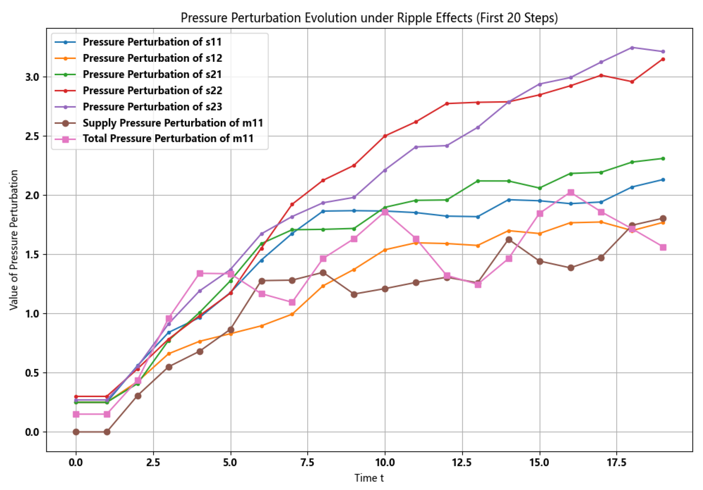
Figure 2 visualizes the SC disruption on the subnetwork $N_1$. This tool clearly identifies both the type and source of supply pressure affecting a given manufacturer. Managers can clearly identify how risks faced by individual members evolve. More importantly, they can intuitively pinpoint the key suppliers responsible for major risks, thereby providing further guidance on how to optimize those suppliers.

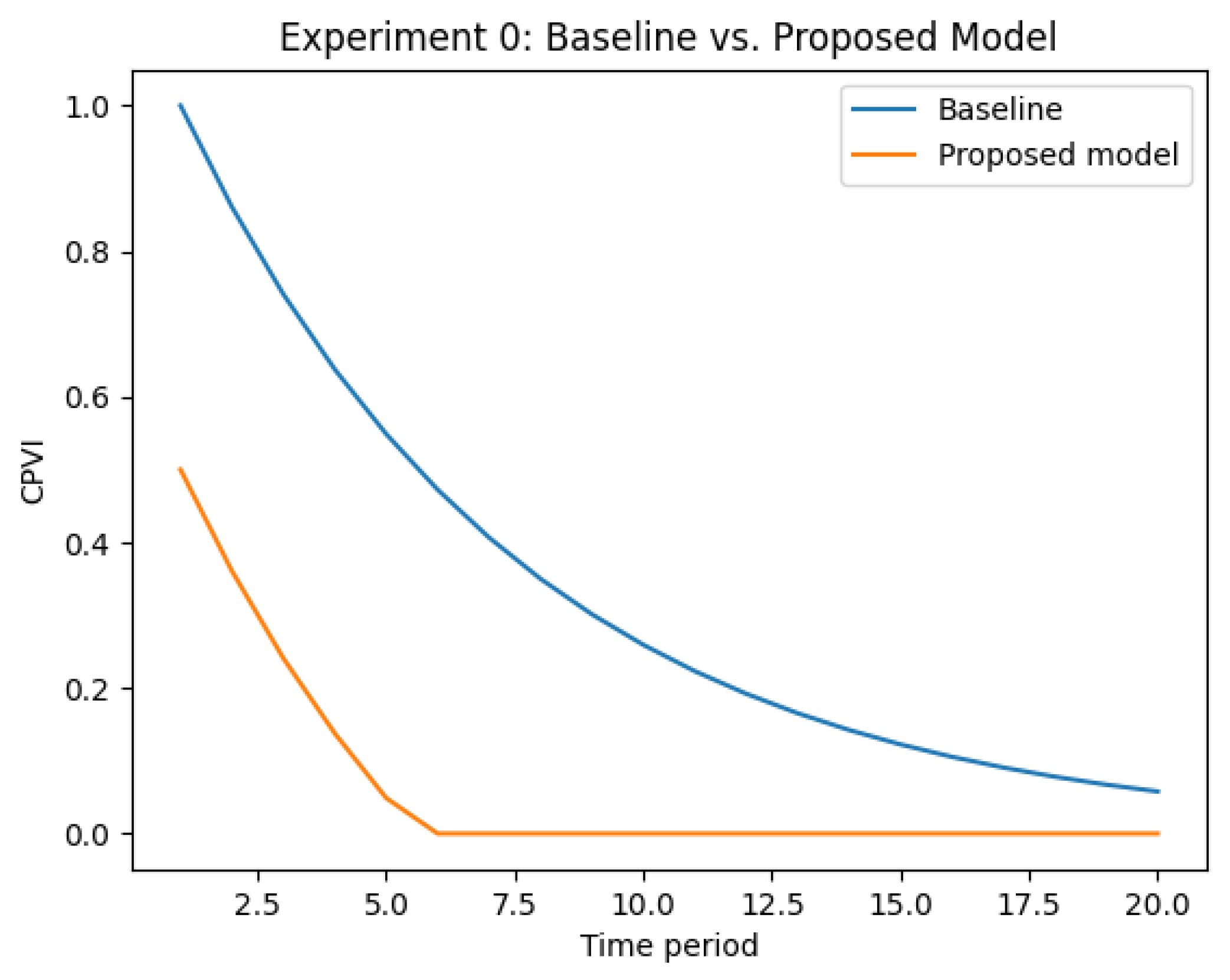
Furthermore, CPVI was employed to compare models with and without mitigation strategies. In this experiment, the risk mitigation inventory is set as a uniformly distributed random variable, thereby allowing risks to continue mitigating gradually. The blue line in Figure 3 represents a simplified model without decision-making, while the orange line represents an optimized model that incorporates decision-making.

As clearly observed from the blue line in Figure 3, even without incorporating inventory levels into the decision model, this pressure wave model demonstrates how risk-mitigating inventory can alleviate risks. Furthermore, when utilizing an optimization model that accounts for inventory levels, the proposed model consistently achieves lower CPVI values than the baseline across all decision periods, demonstrating that endogenous mitigation decisions play a crucial role in suppressing pressure propagation. Compared with methods like Bayesian networks, this stress wave method does not output a series of probability information, but rather visualizes the most likely state of each node.

It can be observed from the results that: (1) methodologically, the proposed model characterizes the disruption status of any SC partner using a series of explicit numerical values, whereas Bayesian network methods typically describe states through probability distributions; (2) in terms of spatio-temporal propagation, the transition of disruption states in our model is governed by physical wave equations, rather than being defined by state-transition probabilities, which provides a more interpretable mechanism for capturing SC disruptions over space and time; (3) this tool can be effectively integrated into mathematical optimization models, thereby guiding decision-makers in formulating risk mitigation strategies.

8.2. Experiment on Decision Variables

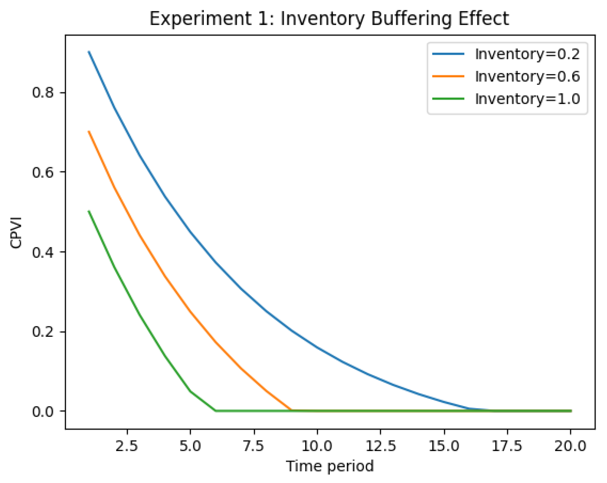
This experiment investigates the impact of inventory buffering on pressure propagation. Different initial inventory levels are considered while all other parameters remain unchanged. In this experiment, inventory levels are set to a fixed value before considering other decision variables. As illustrated in Figure 4, higher inventory levels lead to a pronounced reduction in CPVI throughout the planning horizon. This result confirms that inventory acts as an effective damping mechanism, absorbing upstream pressure shocks and mitigating their downstream amplification.

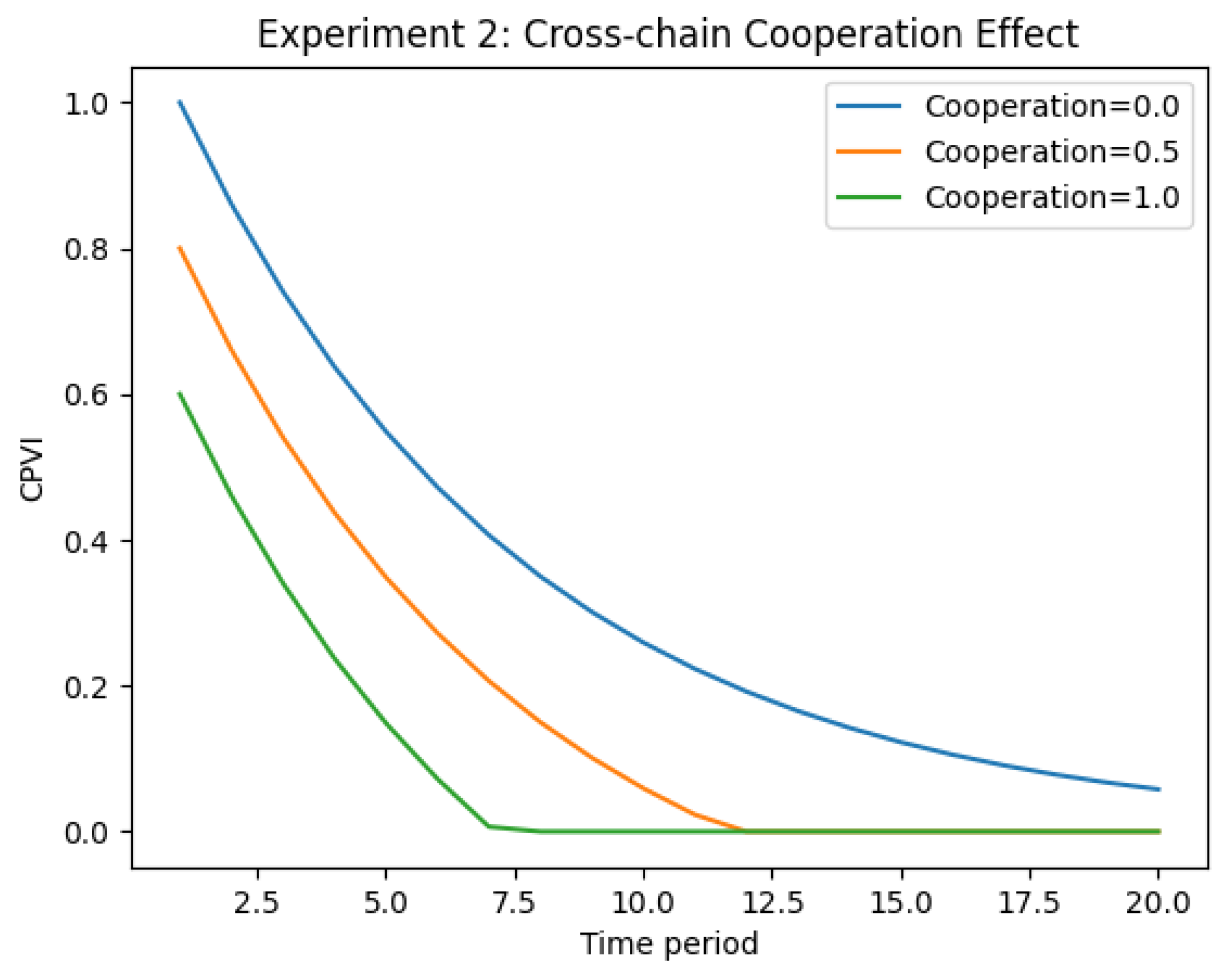
Then we conduct an experiment that evaluates the role of cross-chain cooperation in mitigating systemic risk. Based on Figure 1, it can be seen that manufacturer set $M_1$ can engage in cross-chain collaboration with manufacturer set $M_1$. That is, a total of four manufacturers can choose whether to participate in cross-chain collaboration. The blue, orange, and green curves represent scenarios where cross-chain collaboration is not considered, where collaboration between two manufacturers is considered, and where collaboration between four manufacturers is considered, respectively. The cooperation level determines the extent to which manufacturers are allowed to reallocate orders to alternative subnetworks at an additional cost. In particular, for subnetworks with many stable suppliers, the corresponding manufacturers can adopt a low inventory strategy. Such manufacturers will allocate more production capacity to cross-chain collaborative production.

Figure 5 shows that increasing the level of cross-chain cooperation significantly reduces CPVI, particularly during periods of high upstream pressure. This indicates that structural flexibility provides an effective mechanism for redistributing risk across subnetworks.

It can be observed from the results that: (1) cross-chain collaboration among manufacturers helps rapidly mitigate both localized and systemic SC risks; (2) SCs—particularly CSCN—should incorporate as many members as possible that share proximity in required raw materials; (3) it is important to identify those key suppliers. Components and raw materials that are vulnerable to supply disruptions, such as highly tariff-sensitive components, should be relocated to regions with more stable economic development.

8.3. Optimal Decision Trajectories

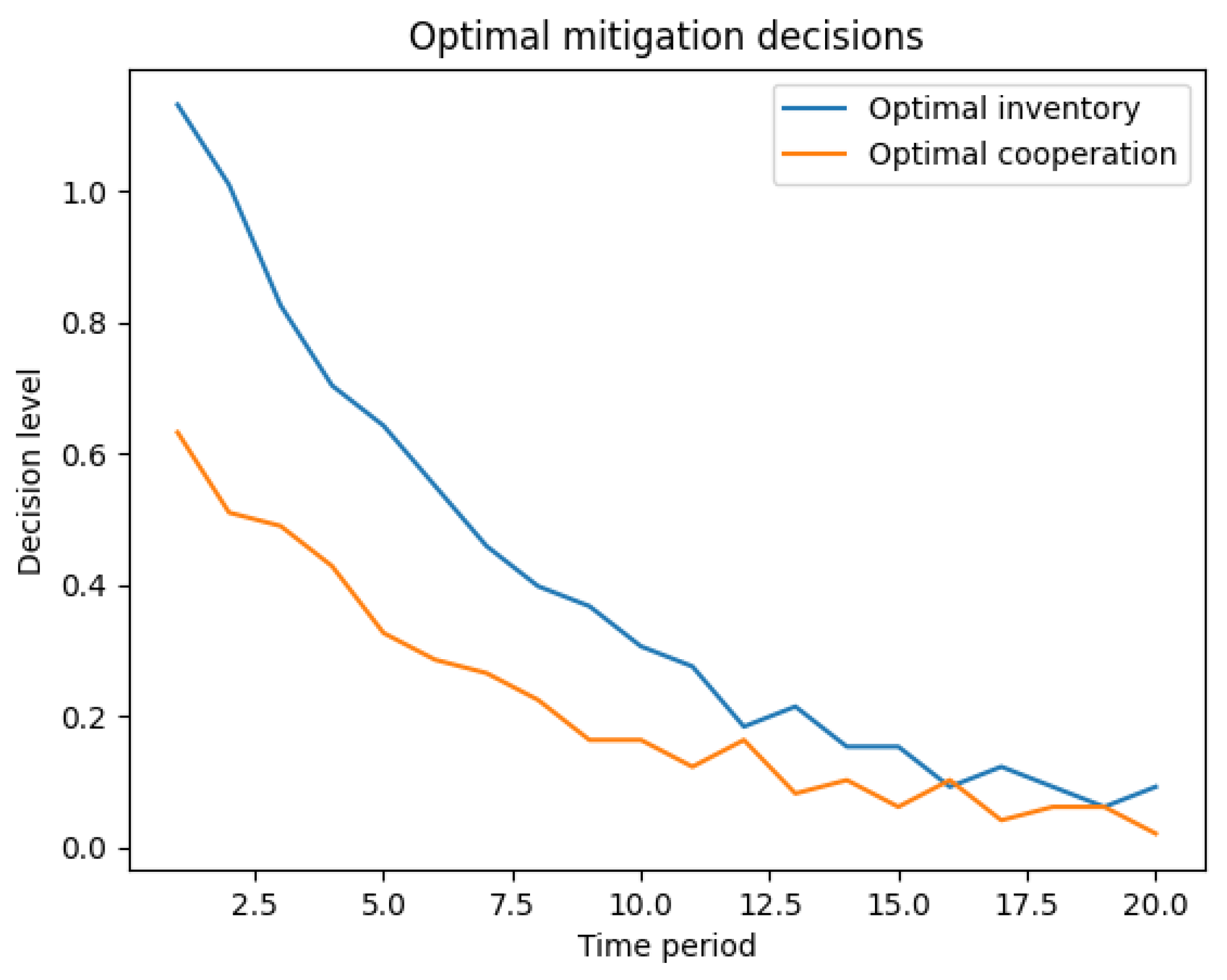
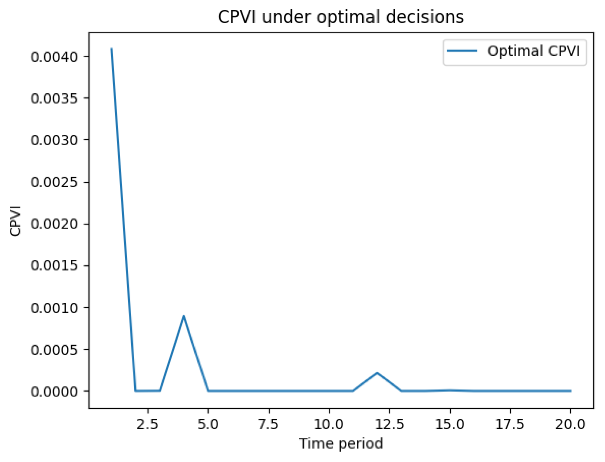
This experiment illustrates the endogenous mitigation decisions generated by the proposed optimization model. Unlike the previous experiments, where mitigation levels are exogenously specified, inventory buffering and cross-chain cooperation are here determined optimally at each decision period. Supplier-side disturbances follow an exponentially decaying pattern, representing a temporary disruption shock. Inventory and cross-chain cooperation decisions are associated with convex mitigation costs, while CPVI enters the objective function to penalize systemic vulnerability.

Figure 6 and Figure 7 report the optimal trajectories of inventory buffering and cross-chain cooperation, while Figure 6 presents the corresponding CPVI evolution. The results show that mitigation decisions are highly time-dependent: both inventory and cooperation levels increase during periods of high upstream pressure and gradually decline as the disturbance weakens. This dynamic adjustment demonstrates the necessity of formulating supply chain risk management as an intertemporal optimization problem rather than a static mitigation strategy.

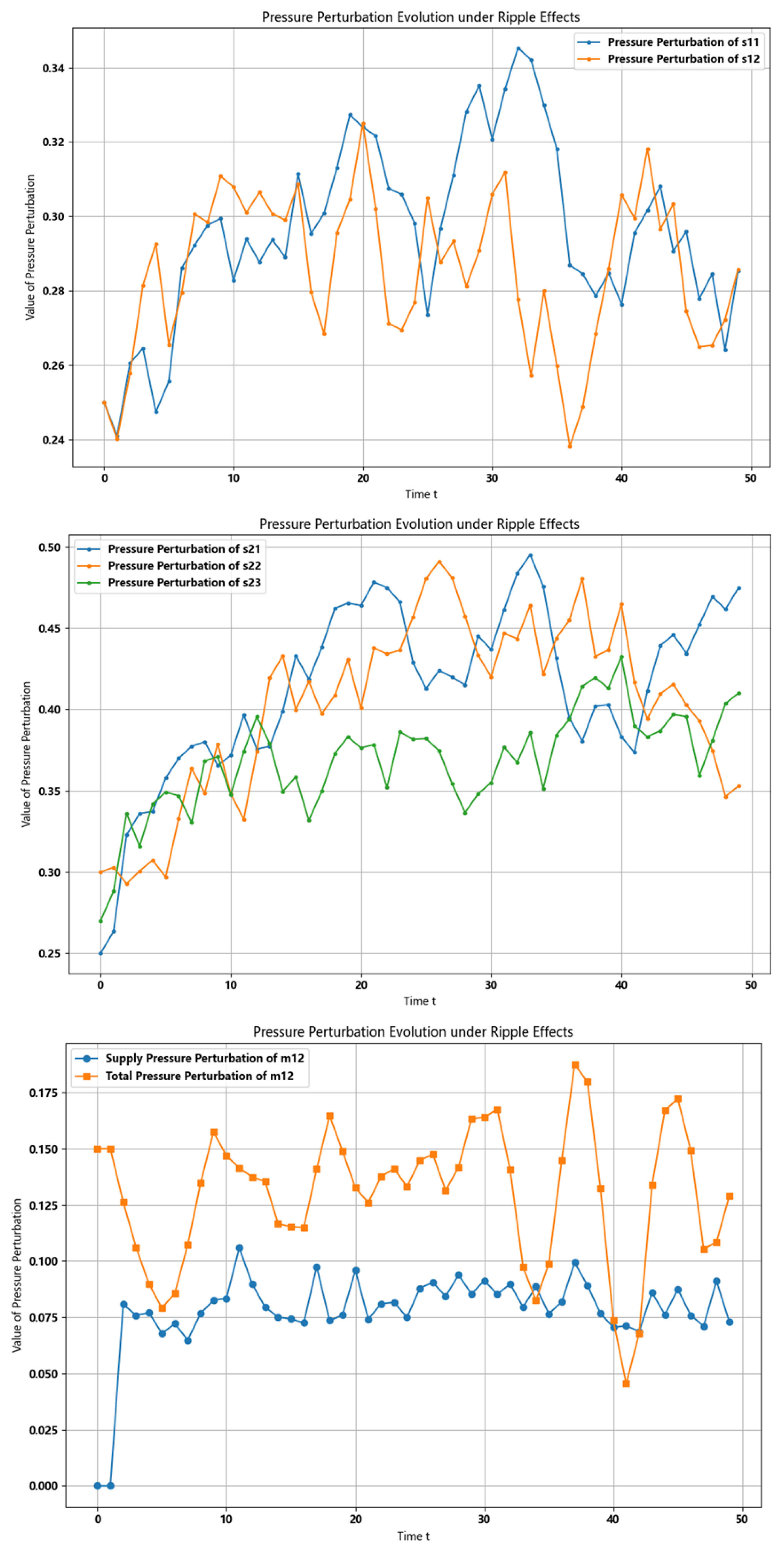
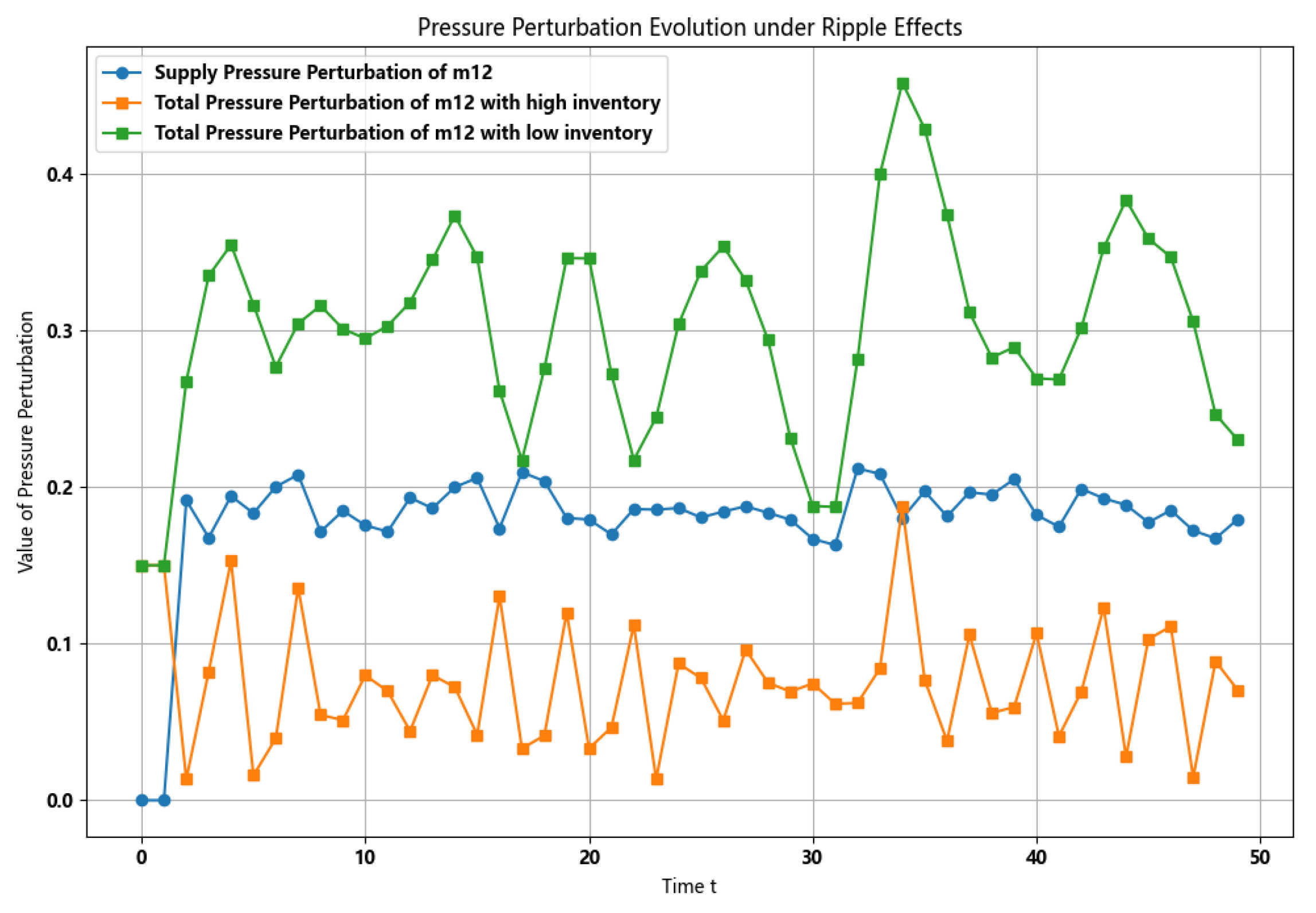
To simulate risk evolution under ripple effects, we construct a model that incorporates a damping term through risk mitigation inventory. A preliminary example illustrates how this inventory functions. The first two graphs in Figure 8 visualize ripple effects on the supplier side, clearly identifying both the type and source of supply pressure affecting a given manufacturer. This enables managers to formulate targeted mitigation strategies based directly on the pressure’s characteristics—an advantage over Bayesian network approaches, which only provide probabilistic estimates of supplier-induced pressure.

The third graph in Figure 8 depicts supply and total disruptions for manufacturer $m_{11}$, where $I_{m_{11}}\left(t\right)\sim U(0.30,0.45)$. As shown, $m_{11}$ is primarily disrupted by supplier set $S_2$, whose maximum disruption fluctuations are smoothed by exponential decay. Due to the low pressure mitigation inventory level, $m_{11}$ cannot fully absorb disruptions from the previous period, resulting in wide fluctuations that reflect the temporal propagation of ripple effects.

Figure 9 compares disruption evolution for $m_{11}$ under different inventory levels. To highlight the damping effect of mitigation inventory, we amplify supply disruptions by adjusting the exponential decay parameters and set $I_{m_{11}}\left(t\right)\sim U(0.30,0.45)$ and $U(0.50,0.65)$, respectively. Although $m_{11}$ experiences identical supply disruptions in both scenarios, the higher inventory level reduces total pressure perturbation by approximately two-thirds. Moreover, increased mitigation inventory stabilizes $m_{11}$ and dampens its response to external disruptions.

9. Conclusions

This paper takes CSCN as an example and investigates a novel pressure wave-based modeling framework to analyze and mitigate bi-directional disruption propagation in CSCN. This paper draws upon pressure wave theory from fluid mechanics to model disruption events as continuous dynamic “pressure” signals propagating both forward and backward within the CSCN. This framework captures a range of factors influencing the propagation pathways and intensity of supply chain risks—such as partner resilience, information-sharing efficiency, and cross-chain interactions—thereby enhancing the interpretability of the model’s physical parameters. To quantify systemic risk, this paper introduces two innovative metrics: SPVI and CPVI, measuring disruption vulnerability at the subnetwork and overall network levels, respectively. Numerical experiments based on real CSCN configurations demonstrate that this model accurately reflects spatiotemporal propagation pathways, evaluates the effectiveness of resilience strategies (such as inventory buffering and supplier reallocation), and reveals management insights supporting disruption response and recovery. More importantly, this approach innovatively integrates physical models with mathematical optimization models. By incorporating risk mitigation strategies—such as inventory levels and cross-chain collaboration—into the physical model, it guides decision-makers toward optimal choices. The model accurately reflects spatio-temporal propagation pathways, evaluates the effectiveness of resilience strategies, and reveals management insights that support disruption response and recovery.

The proposed model has several limitations that point toward valuable directions for future research. The proposed method also has the following limitations. First, the model has not been tested on a sufficient number of real-world cases. Therefore, relevant parameters require further determination using actual data in conjunction with machine learning and other methods. Second, the model considers a two-tier supply chain, and its applicability to supply chain risk propagation mechanisms in multi-tier supply chains remains to be determined. Several avenues for future research remain open. Extensions of the model could incorporate multiple interacting pressure sources, stochastic disturbance processes, or learning-based decision rules under incomplete information. In addition, developing scalable solution algorithms for large-scale industrial networks represents a promising direction for further investigation.