Customer Experience Quality and Its Marketing Outcomes in Banking: Evidence from Industry in Transition

Abstract

Human–technology relationships have become core strategic capabilities and enablers of enterprise sustainability. Contemporary interactions between humans and technology are undergoing a profound transformation toward a more human-centric and value-oriented paradigm, aiming for Industry and Society 5.0, a shift that is particularly salient in banking. The influence of customer experience quality on the strategic foundations of enterprise management is being fundamentally redefined. The purpose of this research is to assess the influence of customer experience on marketing outcomes in the banking industry. To analyze the directions, strengths, and statistical significance of relationships, structural equation modeling (SEM) using partial least squares (PLS) was employed. The research model was tested on a sample of 616 valid responses from customers of banking services in Serbia. The research shows that customer experience positively impacts customer satisfaction, behavioral loyalty intentions, and word-of-mouth, making it a strong predictor of marketing outcomes. The moderating roles of gender, customer segment, and respondents’ regional affiliation were tested, identifying variables that moderate significant relationships between customer experience and marketing outcomes, unveiling detailed insights into demographic and segmentation disparities. The findings offer robust empirical support for managerial decision making in customer experience enhancement initiatives.

1. Introduction

The transition from Industry 4.0 to Industry 5.0 represents a shift from technology-driven automation toward a human-centric, sustainable, and resilient model of industrial development, in which industry assumes a broader societal role by aligning production processes with ecological constraints and employee well-being [1,2]. Observing industrial development over time, five major industrial transformations can be identified. Industry 5.0 is regarded as the next phase of industrial development, with its primary objective to harness human creativity in collaboration with efficient, intelligent, and precise machines. This paradigm assumes the integration of human creativity with powerful, intelligent, and accurate machines, and many technological visionaries argue that Industry 5.0 will restore the “human touch” to industry. Furthermore, Industry 5.0 can enhance production quality by allocating repetitive and standardized tasks to machines, while assigning tasks requiring critical thinking and cognitive judgment to humans.

Although the full implementation of this concept has not yet been achieved, substantial research contributions highlight its potential, particularly in service sectors such as banking, where artificial intelligence and collaborative robotics are redefining the roles of humans and technology in value creation [3,4]. Existing studies emphasize that the successful adoption of Industry 5.0 requires developing new skills through lifelong and interdisciplinary learning, human-centric data governance, and enhanced human–machine interaction, while also raising new research questions about the regulation of these interactions and potential conflicts between humans and artificial intelligence [5].

Banking 5.0 has emerged as a result of an industrial revolution driven by artificial intelligence, similar to previous industrial revolutions that were shaped by other powerful technologies. Banking 5.0 introduces a cultural transformation in customer relationships, shifting the approach from a predominantly passive to a preventive model of operation, accompanied by the development of a wide range of new services and products, innovative business models, and increased attention to default prevention. Customer needs, knowledge, and expectations have expanded exponentially over time, requiring financial institutions to continuously adapt to the demands of contemporary users. In an environment characterized by urgency, constant change, and an abundance of choices, where customer loyalty can no longer be taken for granted, banks must move beyond their core products and services to retain and expand their customer base through innovation and a fundamental transformation of their business approach.

Industry 4.0 can be viewed as supporting the initial phase of the development of the knowledge economy, as it transforms data and explicit knowledge into codified and scalable value through a process encompassing data generation, data analysis, automation, and productivity enhancement, whereby explicit organizational knowledge is embedded into software, algorithms, digital platforms, and process intelligence systems [1]. In contrast, Industry 5.0 represents an evolution of the knowledge economy oriented toward tacit knowledge and the management of intangible capital, redefining value creation beyond technological intensity and mere productivity growth toward responsible innovation that prioritizes human well-being, sustainability, and systemic resilience. Within this framework, competitive advantage increasingly relies on interdisciplinary knowledge that integrates engineering disciplines with the social sciences, ethics, and sustainability, alongside the adoption of new performance indicators and accountability mechanisms, such as ESG metrics, life-cycle assessment, and measures of employee well-being [1]. Accordingly, Industry 5.0 emphasizes the development of human cognitive capabilities, collaboration, creativity, and system-level design thinking as essential complements to automation and digital skills, thereby redefining how knowledge is created, applied, and governed in contemporary economies.

Developed nations started transitioning from an industrial economy to a knowledge-based economy several decades ago, and it’s only now that developing countries are catching up. This delay in shifting to a knowledge economy presents both significant opportunities and challenges for developing nations [6]. By learning from the successes and failures of developed countries during their own transitions, developing nations can avoid mistakes and adopt effective solutions. This enables developing countries to accelerate their development and integrate into the knowledge economy by overcoming the same obstacles that advanced economies have encountered during their own transitions. Besides the global transition towards a knowledge-based economy, developing nations have also undergone an economic transformation that facilitated the inflow of foreign capital via privatization initiatives. This process compelled these countries to compete within markets predominantly occupied by firms from developed economies. Within the framework of a knowledge-based economy and Industry 5.0, customers are regarded as active participants rather than passive consumers, a phenomenon that is especially evident in the service sector [7]. They contribute knowledge, participate in value creation, and drive innovation through interactions and feedback. Their engagement with firms and other customers shapes products, services, and the overall market landscape [8]. Consequently, the relationship between customer experience (CX) and the knowledge economy is gaining importance, as organizations recognize that customer knowledge and CX are key pillars for enhancing customer satisfaction, loyalty, and ultimately, competitive advantage [9]. Modern businesses operating in a knowledge-based economy rely on managing and leveraging customer insights to deliver tailored services and build stronger relationships with customers [10].

As economies mature, the shift occurs away from manufacturing towards service sectors, which influences the structure of employment. In high-income economies, services account for the largest share of GDP, often exceeding two-thirds of total output [11]. According to World Bank data from 2021, the contribution of services to GDP in high-income economies typically exceeds 70%, often reported as 70% to 75%, highlighting the sector’s importance in economic activity and development [12,13]. Serbia is currently classified as an upper-middle-income country. The value of services contributing to GDP in the Republic of Serbia in 2001 was 41.89 per cent, while the maximum of 58.54 per cent was recorded in 2024 [14].

Customer satisfaction was historically neglected within a distinctive model of market socialism that characterized Serbia’s economic landscape. In this framework, consumer choice was largely irrelevant, even as demand consistently exceeded supply, rendering customer satisfaction a secondary concern for producers. The transition to a market-oriented economy introduced competitive dynamics and consumer sovereignty, thereby elevating customer satisfaction to a central focus in both business practice and academic discourse [15,16].

During Serbia’s transition from a self-managed socialist economy to a market-oriented system, the banking sector underwent significant foreign influence characterized by mergers and acquisitions involving domestic financial institutions. The entry of financial entities from highly developed, digitized economies occurred rapidly, posing considerable challenges for banking personnel and clientele due to the novelty of digital technologies. This transition period required comprehensive adaptation, including technological upgrades, process reengineering, personnel training, and customer education to facilitate effective integration [17]. The disparity in digitalization levels between local markets, such as Serbia, and the ecosystems of international banking institutions, coupled with a limited comprehension of the determinants of customer satisfaction, has the potential to undermine competitive advantages even for market leaders. Consequently, marketing strategies that are effective in banks’ domestic markets may not necessarily yield the same results in the Serbian context [18]. To attract and retain customers, banks must identify the key factors that influence customer experience, satisfaction, loyalty, and word-of-mouth behavior. Customer experience can be considered a critical determinant of customer behavior [19], encompassing all interactions a customer has with an organization, including engagement with products and services and all brand touchpoints [19,20]. As the service economy expands, understanding and managing CX is crucial for achieving a competitive advantage. Increasing competition, combined with increasingly sophisticated customer expectations, necessitates that organizations prioritize the provision of exceptional experiences to differentiate themselves in the marketplace. Customer experience has shifted from a buzzword to a key marketing and business practice, becoming a top priority for both businesses and academia [21,22].

However, although CX is a comprehensive and integral concept encompassing affective, cognitive, and behavioral aspects, the existing literature remains fragmented and requires further development. The relationship between CX and marketing outcomes in the banking sector is crucial for developing effective marketing strategies that enhance overall operational performance. In a competitive environment, delivering a personalized CX is indispensable, as it directly affects marketing results [23]. The development of CX as a competitive battlefield highlights a shift from simply providing good service towards a comprehensive assessment of customer interactions [24]. A renewed emphasis on measuring CX and connecting these metrics to vital marketing outcomes, such as customer advocacy and loyalty, is essential. This aligns with findings that a well-measured CX can drive significant corporate success, thereby stressing the need for banks to adopt better measurement techniques [25,26,27].

Optimizing CX has emerged as a primary strategic focus for companies, emphasizing the expansion of interaction modalities that allow customers increased autonomy and flexibility in accessing support and information [28,29,30]. All service providers utilizing electronic channels for customer interaction invest considerable effort in aligning their operational procedures with customer expectations, intending to attain a high degree of customer satisfaction [31].

Some of the work published on the CX and customer satisfaction in the service sector was focused on insurance services [25,32,33], hospitality and tourism [34,35,36,37] and e-commerce [38,39,40]. Papers highlighting the impact of CX in the financial sector, including banking, insurance, and investment, have gained notable attention in academic research on customer satisfaction. It was shown that high service quality correlates positively with customer satisfaction, establishing that service excellence leads to customer loyalty [41]. Some scholars have dedicated their research efforts to examining CX within the banking sectors of emerging markets [42,43,44].

The banking sector is essential for emerging economies and is undergoing rapid digitalization amid fierce competition. As of March 2024, approximately 20 licensed commercial banks in Serbia have continued consolidating through mergers and acquisitions (M&A). Total sector assets reached EUR 55.8 billion by the end of 2024, up from EUR 42.9 billion in 2021. The top 10 banks hold approximately 91% of assets, with ongoing M&A activity likely to maintain or increase this concentration. Only two banks, Poštanska štedionica and one smaller state-owned bank, are majority Serbian-owned, while others are affiliates of European banking groups. Research on customer satisfaction in the Serbian banking sector is limited [17,18,45]. This research gap presents an opportunity to examine the broader scope of the CX phenomenon and its marketing implications, considering the distinctions between specific customer segments, namely retail and business.

This study aims to address gaps in scholarly literature by systematically examining the dominant influence of CX on marketing outcomes. Consequently, it seeks to develop evidence-based guidelines and strategic recommendations to help banking institutions improve their service quality, enhance CX and satisfaction, and secure a sustainable competitive advantage in emerging markets. Using Structural Equation Modeling (SEM) in SMART-PLS 4.1, the researchers analyzed data from banking service customers. The analysis examined the moderating effects of demographic variables, including gender, customer segments, and regional affiliation. By clarifying the significant connections between CX and marketing outcomes, as well as how demographic factors influence these relationships, this study deepens the understanding of interactions among banking consumers in developing markets. The findings provide valuable insights into tailoring marketing strategies to various customer segments and regional contexts.

The following section provides a comprehensive review of the relevant literature, highlighting key research advances and main theoretical frameworks related to the subject. The next section of the paper outlines the research methodology, offering detailed descriptions of the sample, measurement techniques, and analytical procedures used. The final section discusses and synthesizes the findings, including implications for future research and practical applications in the banking sector.

2. Literature Review

Understanding CX and the customer journey over time is crucial for organizations. Customers now interact with firms through multiple touchpoints across different channels and media, and their experiences are becoming more social in nature [19,46].

Leading service companies aim to enhance their primary customer journeys, as improved performance in these areas is linked to higher customer satisfaction and business growth [47,48]. Thus, companies must systematically gather insights into the dynamic nature of customers’ experiences to facilitate the meticulous design, coordination, and management of the various components of their journey. Additionally, they should develop rigorous mechanisms for ongoing monitoring and evaluation of CX throughout the customer journey [49].

A literature review exploring CX quality through the lens of the Customer Experience Quality (EXQ) scale [50] across various industries and emerging markets reveals critical insights into how companies can strategically enhance customer interactions to foster loyalty and satisfaction. Furthermore, the EXQ scale has undergone evaluation across diverse customer segments, demonstrating that although CX characteristics may vary by cultural context, the fundamental dimensions used for experience assessment remain consistent [51,52].

The EXQ scale was established as a robust framework for measuring CX across diverse sectors, including healthcare [53,54], hospitality, and banking [23]. In healthcare, for instance, adapting the EXQ scale to evaluate patient satisfaction demonstrates its versatility, promoting a positive correlation between patient experience perceptions and loyalty. Similarly, in retail banking, studies employing the EXQ scale illustrate its efficacy in assessing service quality perceptions, enabling institutions to refine their customer engagement strategies [42].

The principal contribution of this study is to offer comprehensive insights and empirical data that advance research on CX and its marketing outcomes within the banking sector, with a particular focus on the Serbian context.

Since the standardized EXQ scale was used in this study, the findings can be compared with those of earlier studies using the same instrument. The results from analyzing the interaction among key dimensions of CX, namely, brand experience, service (provider) experience, post-purchase/consumption experience, alongside customer satisfaction, behavioral loyalty intentions, and word-of-mouth, should lead to effective managerial strategies.

2.1. Dimensions of Customer Experience

This paper is based on the EXQ framework of CX [55]. Since its initial development and validation, the Customer Experience Quality (EXQ) scale has been empirically tested across numerous studies [56], confirming its factorial structure and predictive validity.

Authors [57] have inquired about the extent to which the EXQ scale needs to be adapted, considering social and economic differences, especially the challenges faced by consumers in emerging economies such as Serbia. They have found that, using the modified EXQ scale, it is possible to identify and measure brand experience, service (provider) experience, and post-purchase/consumption experience as dimensions of CX within the banking sector in Serbia.

2.1.1. Brand Experience

The Brand Experience (BRE) dimension in the EXQ scale [24,50] is a vital element for assessing in services. Brand experience includes sensory, affective, cognitive, and behavioral responses to a brand, shaping consumer behavior [58,59,60,61]. This construct is vital as it captures a comprehensive interaction consumers have with brands. Unlike traditional service quality models (such as SERVQUAL), the BRE dimension of the EXQ scale includes seven items that highlight aspects valued by customers beyond simple satisfaction, specifically, the cognitive, emotional, and brand-related judgments they form throughout the customer journey. Brand image and trust are foundational to reputation. They can serve as a shortcut to reducing perceived risk in business, especially in services where quality cannot be assessed visibly, and a strong brand reputation signals reliability and value. Furthermore, brand credibility is perceived as competence or expertise that fosters customer confidence and affects purchase intentions [62,63,64]. Brand credibility is widely recognized as a critical determinant of consumer decision-making, especially in markets where risk and information asymmetry are high [65]. A central component of brand credibility is perceived competence or expertise, which refers to the extent to which consumers believe that the brand has the necessary skills, knowledge, and ability to deliver on its promises [66]. This perception of competence fosters customer confidence, reduces uncertainty, and enhances the brand’s perceived reliability. In service settings, such as banking or healthcare, where the intangibility and complexity of the offering make it difficult for customers to assess quality before consumption, the brand’s perceived expertise acts as a signal of expected performance [67].

According to the relationship marketing literature [68,69,70,71], perceived fairness and customer advocacy lead to deeper trust [72] and loyalty. Independence in advice enhances perceived authenticity of the brand, reflecting benevolence, an essential component of trust, and customer-oriented behavior [73,74,75,76].

The connection between brand experience and EXQ can be illustrated through various studies exploring the dynamics of consumer interactions and the resulting levels of satisfaction, loyalty, and advocacy. For instance, the integration of mediating variables, such as brand love, can amplify the understanding of how brand experiences enhance loyalty [77,78].

2.1.2. Service (Provider) Experience

The Service (Provider) Experience (SPE) dimension of the EXQ scale is vital for comprehending the quality of customer interactions within service environments. Empirical validations and adaptations across diverse sectors, beyond traditional service industries like healthcare, have further substantiated its significance in sports management and healthcare, reinforcing its utility in advancing both theory and practice in service marketing [79]. Therefore, using the EXQ scale can significantly improve firms’ capacity to create and provide more engaging and satisfactory service experiences, ultimately resulting in higher customer loyalty and positive business results [51,56].

The SPE dimension of the EXQ scale assesses the quality of interactions between a customer and a service provider throughout the customer’s journey. This dimension is evaluated by eleven items that measure customer-perceived value, emphasizing how the firm advises, supports, adapts, and connects with individual customer needs.

Through companies’ proactive engagement in value-creating processes [80] customers perceive enhanced relational and functional value, as they feel supported, informed, and empowered throughout their entire journey [81,82]. The customer’s perception of the effort involved in using a service significantly influences satisfaction and repurchase [83] and could be considered as an accurate predictor of loyalty [84].

The companies’ effort to provide customers with timely, accurate, and relevant information [85] enhances the customer’s ability to understand and engage with the service process [86,87] signaling reliability, competence, and openness, which are core to trust formation [88], emotional connection [89] and satisfaction [85,90]. Familiarity with personnel and processes is a key antecedent of trust [91] and emotional attachment [92] that fosters personalization and recognition, constituting a crucial indicator of customer-centricity [93], reinforcing customer comfort and mitigating friction in service consumption [94]. Together, these elements foster both practical and emotional loyalty [95,96], resulting in greater customer retention, increased share of wallet, and positive word-of-mouth.

Personal relationships between customers and service personnel foster affective trust [71], characterized by emotional bonds, familiarity, and a sense of interpersonal understanding [97,98]. In high-contact services such as banking, healthcare, or consulting, these relationships [89] are crucial in shaping customer perception by providing consistency, emotional support, and care. They strengthen relational bonds, boosting loyalty behaviors like re-purchase, lower price sensitivity, and positive word-of-mouth [99].

A superior service environment [100] improves customer evaluation of the service and boosts differentiation-based value perceptions [72,101]. The customer’s view of the efficiency and convenience of the service environment, offline or online, is essential. Well-designed service delivery platforms, especially online [94], enhance perceived value by reducing effort, boosting the convenience of the CX [83].

2.1.3. Post-Purchase/Consumption Experience

The Post-Purchase/Consumption Experience (PPE) dimension of the EXQ scale is vital to the customer journey, as it impacts satisfaction and loyalty. It highlights factors such as usability, support, and post-purchase fulfillment. The PPE in the EXQ scale reflects customers’ long-term evaluations of satisfaction, perceived attention, and loyalty, measured by seven items.

Understanding and responding to individual needs is key to high-quality service relationships, mainly when customer retention depends on consistent personalized experiences [19,102,103,104,105] which is especially important in high-contact services, such as banking, healthcare, or consulting, where repeated interactions enable firms to gain valuable customer knowledge [106,107,108,109]. Such familiarity enables tailored service and signals emotional investment, boosting affective commitment [99]. Consequently, customers experience less relational uncertainty and greater trust, which in turn boosts psychological switching costs and encourages long-term loyalty [110] that aligns with established theories in consumer psychology and relationship marketing [110,111]. Moreover, empirical studies confirm that customers are more likely to remain loyal to service providers who demonstrate an ability to remember, anticipate, and adapt to their evolving needs [111,112,113]. This form of tailored service increases switching costs, strengthens customer satisfaction, and enhances relational loyalty [70,114].

From a strategic perspective, customers who perceive that a firm is committed to sustaining the relationship beyond immediate transactions are more inclined to develop relational commitment. This commitment is characterized by emotional attachment, diminished motivation to switch providers, and increased tolerance for service failures [99,110]. Furthermore, these perceptions may facilitate customer advocacy behaviors, such as the dissemination of positive word-of-mouth and the willingness to offer constructive feedback, thereby fostering the firm’s sustainable value creation [115].

From a strategic perspective, effective service recovery efforts signal organizational competence, customer-centricity, and accountability [116,117]. These attributes collectively foster enduring customer loyalty [118]. In high-involvement service contexts, particularly where establishing trust and mitigating perceived risks are critical, the capacity to manage adverse situations effectively emerges as a crucial factor influencing emotional commitment and subsequent repurchase [119,120,121,122].

When a customer reports being “happy” with a service provider, this reflects not only functional satisfaction with service outcomes but also emotional contentment with the overall relationship, including communication, personalization, and recovery performance [123,124]. This form of post-consumption contentment has been empirically shown to influence both attitudinal and behavioral loyalty, making it a key predictor of retention, cross-buying, and advocacy [125,126]. Moreover, satisfied customers often act as informal brand ambassadors, voluntarily spreading positive word-of-mouth, which serves as a powerful form of peer influence in service markets and is essential to understanding long-term service outcomes [127].

In services marketing, particularly within high-involvement, high-status, or luxury sectors (e.g., private banking, consulting, elite education, or high-end retail), the company becomes a social symbol. Social approval is one of the key drivers of status consumption, wherein consumers use brands and services to communicate identity, prestige, and affiliation [128]. Customers often derive value not only from the functional attributes of the service but also from the social meaning associated with being a client of a prestigious or widely respected provider [129]. This value is externally oriented, as it concerns how others perceive the customer’s choice and relationship with the brand or service firm. Empirical research supports the notion that social approval influences post-purchase behaviors, such as brand attachment, loyalty, and word-of-mouth communication [130,131].

Industry 5.0 offers a relevant theoretical framework for interpreting Customer Experience Quality (EXQ) in the banking sector, as its core principles closely correspond to the multidimensional structure of the EXQ construct. The principle of human-centricity, which places human needs, trust, and well-being at the center of value creation, is strongly reflected in the Service Provider Experience (SPE) dimension, emphasizing interpersonal interactions, empathy, and relational quality in service encounters [56]. The notion of human–technology collaboration, a defining feature of Industry 5.0, aligns with the Product and Process Experience (PPE) dimension, where digital technologies and service processes are designed to augment human decision-making and support personalized, seamless customer journeys rather than purely efficiency-driven automation [2,4]. Finally, the Industry 5.0 emphasis on sustainability, resilience, and long-term value creation resonates with the Brand Relationship Experience (BRE) dimension, which captures customers’ emotional attachment, perceived integrity, and long-term trust in the bank as an institution [24]. Collectively, these linkages position EXQ as a theoretically grounded operationalization of Industry 5.0 principles in the banking context, reinforcing customer-centricity as the central mechanism for integrating human, technological, and ethical considerations into contemporary banking experiences.

Based on the literature review encompassing brand experience, service (provider) experience, and post-purchase/consumption experience, it is evident that numerous scholars highlight the significance of these dimensions within the customer journey. Moreover, they emphasize their substantial influence on the overall CX. Consequently, the authors propose the following hypothesis:

Hypothesis 1. 

Brand experience, service (provider) experience, and post-purchase/consumption experience have a positive influence on customer experience.

2.2. Aspects of Marketing Outcome

Based on an extensive review of the existing literature on marketing outcomes associated with CX, the authors adopted and adapted the following aspects: customer satisfaction, behavioral loyalty intentions, and word-of-mouth. The scale is referred to as “The Marketing Outcomes of Customer Experience Scale” (MOCE scale).

2.2.1. Customer Satisfaction

The Customer Satisfaction (SAT) included in the MOCE scale, initially developed by Dagger et al., consists of five items [132,133,134,135]. This scale was initially designed for the health care sector, but its applicability has been demonstrated across various industries (e.g., banking, private aviation, travel) [132,136,137,138,139].

SAT items reflect and measure various psychological constructs, including emotional valence, which indicates a general positive emotional attitude toward the service provider, and capture emotional affinity [140]. Respondents’ ease in interactions and their perception of familiarity pertain to the overall quality of interactions within Dagger’s comprehensive framework. Integrative satisfaction is the anchor item in most applications, aligning with global satisfaction judgments [134], while performance adequacy explains experience-based outcomes [141]. The gap closure between customer expectations and perceived results is key for modelling expectation sensitivity and defining satisfaction [142].

Based on the literature review encompassing customer satisfaction, it is evident that numerous scholars highlight the significance of this aspect of marketing outcome. Moreover, they emphasize the substantial influence of CX on customer satisfaction. Consequently, the authors propose the following hypothesis:

Hypothesis 2. 

Customer experience has a positive influence on customer satisfaction.

2.2.2. Behavioral Loyalty Intentions

The Behavioral Loyalty Intentions (L) items, included in the MOCE scale, highlight the link between CX and customer satisfaction, trust, and loyalty intentions [143]. In a changing marketplace, understanding the dynamics of this scale is crucial for businesses seeking to cultivate long-lasting customer relationships. The research built upon this foundational framework provides insights into applications across various contexts and confirms the importance of understanding the complexities of consumer loyalty.

The core idea of the L scale indicates that satisfied customers are more likely to show greater loyalty to a provider [144], emphasizing interconnectedness of the aspects of satisfaction and loyalty, broadening the fundamental theories stating that higher satisfaction positively affects trust and loyalty, supporting its role as a key variable [70], or stronger customer-provider relationships that are likely to boost loyalty [145].

The perceptual aspects of relationship quality and post-purchase perceived value [146] reinforce the idea that relationship quality serves as a precursor to loyalty intentions. The automatic emotional responses consumers have towards brands indicate that emotional bonds are crucial for perceived relationship quality and, consequently, for repurchase intentions. This affirms the idea that emotional engagement, rather than just transactional experiences, shapes the loyalty landscape [145] through the Behavioral Loyalty Intentions scale.

A more comprehensive understanding of CX and loyalty intentions suggests that service quality exerts a substantial influence on customer satisfaction and trust, which are fundamental for fostering customer loyalty [147].

Overall, the evolving discourse surrounding the L scale illustrates its adaptability to new contexts and its integration with related constructs such as trust, relationship quality, and emotional engagement. By synthesizing contemporary research, the L scale has become one of the most widely adopted tools for measuring customers’ future behavioral intentions in service marketing. This scale aims to capture not actual behavior, but customers’ intentions to engage in behaviors indicative of loyalty, including word-of-mouth recommendations, repurchases, and increased usage.

Based on the literature review encompassing behavior loyalty intentions and their correlation with CX, the authors propose the following hypothesis:

Hypothesis 3. 

Customer experience has a positive influence on behavioral loyalty intentions.

2.2.3. Word-of-Mouth

The word-of-mouth (WOM) items included in the MOCE scale highlight the importance of WOM in consumers’ decision-making processes across different contexts, spreading significance beyond academia into practical marketing strategies, reinforcing the necessity for businesses to recognize and foster positive WOM as a marketing strategy [148].

A study on positive WOM behavior has significantly contributed to understanding the antecedents of consumer engagement in WOM communication, particularly within a retail context [149]. This research underscored the significance of multiple psychographic variables, notably consumer identification and commitment, acting as mediators in the relation between satisfaction and positive WOM intentions. A comprehensive theoretical framework was proposed that elucidates these dynamics by incorporating various antecedent factors that influence individuals’ propensity to engage in WOM behaviors, thereby enhancing the robustness of consumer-business relational ties.

Subsequent studies have investigated the role of service quality, customer satisfaction, and loyalty in driving WOM behavior. For instance, service quality and customer commitment were identified to be antecedents to WOM, thereby solidifying the position of consumer satisfaction as a cornerstone in understanding WOM communication [150]. Similarly, a positive WOM was determined to act as a crucial source of information for potential consumers, especially when previous experiences with a product or service are limited [151]. This emphasizes the influence of existing customer commitment and its role in further spreading WOM communications, aligning closely with the provided framework [149].

Furthermore, the integration of emotional factors within the WOM discourse has also emerged through various studies. For instance, the emotional responses of consumers [152] demonstrate how feelings of gratitude can lead to increased positive WOM, proving that emotional satisfaction plays a crucial role in motivating WOM sharing. Moreover, the exploration of factors influencing negative WOM communication [153] provides a counter-narrative that emphasizes the complexity of consumer behaviors surrounding WOM and illustrates the importance of understanding both positive and negative perspectives within this scope [153,154].

Overall, the convergence of findings highlights the complex nature of WOM behavior, in which both attitudinal and emotional aspects interact with contextual factors such as service quality and customer loyalty to influence consumer behavior. This synthesis stresses the importance of continuous research and adapting marketing strategies to these evolving insights into WOM dynamics.

Sharing product information online with others (eWOM) should be considered a social activity, like other social activities, that is planned (i.e., not random). Since it is driven by extrinsic rewards such as social benefits and economic incentives [155,156], it should be described in social contexts.

Based on the literature review encompassing word-of-mouth and its correlation with CX, the authors propose the following hypothesis:

Hypothesis 4. 

Customer experience has a positive influence on word-of-mouth.

2.3. Moderating Effects

The body of literature pertinent to the CX domain encompasses pivotal research studies concerning CX and its impact on marketing outcomes. These studies primarily investigate and validate the causal relationships between antecedents and outcomes, frequently utilizing variance-based structural equation modeling. Following the determination of causal structures, research endeavors often focus on examining interaction effects. Moderators are recognized as systematic influencers that modulate the strength and, occasionally, the nature of primary effects.

Variables selected as moderators may include categorical variables measured on a nominal scale, such as demographic characteristics of customers. A nominal attribute that partitions customers into discrete groups could be star-rating tiers in hospitality, which reorder the salience of service-quality dimensions for satisfaction [35]. Furthermore, cohort segments shift effective thresholds in the satisfaction and repurchase relation, resulting in nonparallel purchase probability functions across groups [112]. At broader ecosystem levels, country-income groupings differentially weigh the elasticities linking trust, risk, security, and eWOM to purchasing, indicating that the same antecedents carry distinct strengths across macro contexts [119].

Furthermore, variables selected as moderators may include specific sets of items that constitute a construct affecting the structural relationships within the model, thereby facilitating the modulation of effect transmission along the causal path. Competitive intensity amplifies the returns of service and marketing innovation for satisfaction and rivalry relationship, increasing the marginal effectiveness of innovating [41]. A supportive organizational culture strengthens the knowledge-sharing and agility path, converting shared knowledge into adaptive capability [157]. Individual-difference variables, such as epistemic motivation, can attenuate interpersonal routes to engagement (e.g., via customer–employee identification) while leaving firm-identification effects intact, indicating dual mechanisms that are moderated unequally [52]. In digital commerce, accumulated online experience conditions which website attributes matter most, implying that user experience levers should be segmented by experience level rather than optimized uniformly [38].

Within the scope of this research, the potential moderating influence of categorical variables on the relationships between CX and the aspects of marketing outcomes of CX was examined. As moderating variables, the customer’s demographic characteristics were selected. Categorical variables specifying differences among customers of the banking sector, namely, gender, customer segments, and regional affiliation, were selected. Based on the literature review encompassing moderation effects on structural relations of the models, the authors propose the following hypotheses:

Hypothesis 5. 

Customer segment has a moderating effect on the relationship between customer experience and customer satisfaction.

Hypothesis 6. 

Gender has a moderating effect on the relationship between customer experience and customer satisfaction.

Hypothesis 7. 

Regional affiliation has a moderating effect on the relationship between customer experience and customer satisfaction.

3. Materials and Methods

3.1. Instrument

The EXQ scale is a questionnaire designed to provide a systematic, reliable measure of various aspects of CX. Initially, it was conceptualized to assess four distinct dimensions of the CX: aesthetic, emotional, functional, and social [50,55,56,141]. Each of these dimensions is integral to a comprehensive understanding of how users perceive their interactions with a brand or product. Nevertheless, considering the rapid evolution of technology, shifting customer preferences, and emerging market trends, it was necessary to re-evaluate the scale and explore potential enhancements to the EXQ instrument. This is essential to maintaining its relevance and efficacy in accurately measuring and analyzing contemporary CX.

The revised, standardized, and empirically validated instrument, known as the EXQ scale, has been extensively employed across numerous studies [44,158,159]. In the present research conducted in Serbia, this instrument was also utilized. The scale consists of 25 items designed to assess respondents’ attitudes across three distinct dimensions of CX: seven items pertaining to Brand Experience (BRE), eleven items concerning Service (Provider) Experience (SPE) during the delivery process, and seven items capturing perceptions related to Post-purchase Experience (PPE). An adapted version of this scale was proven to be adequate for the Serbian context [57], in which six items pertaining to Brand Experience (BRE), eight concerning Service (Provider) Experience (SPE) during the delivery process, and six items capturing perceptions related to Post-purchase Experience (PPE) were validated (Appendix A,

Table A1. Convergent and Discriminant Validity of the EXQ Scale.

Construct	Item	Standardized Loading	t-Value	AVE	CR	Cα
Brand Experience	6			0.628	0.881	0.884
I am confident in XYZ’s expertise	BRE2	0.789 ***	45.301
XYZ gives independent advice (on which product/service will best suit my needs)	BRE3	0.800 ***	47.272
I chose XYZ not because of the price alone	BRE4	0.710 ***	26.916
The people who work at XYZ represent the XYZ brand well	BRE5	0.832 ***	56.863
XYZ’s offerings have the best quality	BRE6	0.816 ***	44.392
XYZ’s offerings are superior	BRE7	0.801 ***	41.419
Service (Provider) Experience	8			0.631	0.916	0.919
XYZ advised me throughout the process	SPE1	0.821 ***	46.975
Dealing with XYZ is easy	SPE2	0.763 ***	37.335
XYZ demonstrates flexibility in dealing with me	SPE4	0.823 ***	52.797
At XYZ I always deal with the same forms and/or same people	SPE5	0.735 ***	32.661
XYZ’s personnel relates to my wishes and concerns	SPE6	0.821 ***	48.062
XYZ’s personnel relates to my wishes and concerns	SPE7	0.801 ***	41.725
XYZ delivers a good customer service	SPE8	0.853 ***	67.216
XYZ’s (online and/or offline) facilities are designed to be as efficient as possible	SPE11	0.731 ***	29.974
Post-Purchase/Consumption Experience	6			0.668	0.900	0.902
I stay with XYZ because they know me	PPE1	0.789 ***	42.029
XYZ knows exactly what I want	PPE2	0.749 ***	38.007
XYZ keeps me up to date	PPE3	0.799 ***	42.039
XYZ will look after me for a long time	PPE4	0.866 ***	70.660
XYZ deal(t) well with me when things go(went) wrong	PPE5	0.830 ***	54.588
I am happy with XYZ as my (service firm)	PPE6	0.865 ***	69.983

Note: asterisks are used to visually denote the statistical significance of a result, with *** for p < 0.001 (highly significant)

).

The marketing outcomes of CX have also been conceptualized and empirically validated in numerous scholarly studies [132,136,137,138,139,160]. “The Marketing Outcomes of Customer Experience scale”, comprising previously validated and independently developed instruments, was employed to measure marketing outcomes. Five items measuring Customer Satisfaction (SAT) were adopted from the study by Dagger et al. [132]. Another five items capture Behavioral Loyalty Intentions (L), initially applied in studies by Zeithaml et al. [145] and later by Parasuraman et al. [147]. Finally, seven items that measure Word-of-mouth (WOM) were applied from the instrument developed by Brown et al. [149]. An adapted version of this scale was proven to be adequate for the Serbian context, which included five items related to Customer Satisfaction (SAT), five concerning Behavioral Loyalty Intentions (L), and five items capturing perceptions related to Word-of-mouth (WOM) (Appendix A,

Table A2. Convergent and discriminant validity of the MOCE scale.

Construct	Item	Standardized Loading	t-Value	AVE	CR	Cα
Customer Experience	3			0.856	0.919	0.916
Brand Experience	BRE	0.909 ***	93.826
Service (Provider) Experience	SPE	0.938 ***	180.700
Post-Purchase/Consumption Experience	PPE	0.929 ***	154.489
Customer Satisfaction	5			0.761	0.922	0.921
My feelings towards XYZ are very positive	SAT1	0.872 ***	73.107
I feel good about coming to XYZ for the offerings I am looking for	SAT2	0.857 ***	58.577
Overall, I am satisfied with XYZ and the service they provide	SAT3	0.856 ***	57.675
I feel satisfied that XYZ produce the best results that can be achieved for me	SAT4	0.894 ***	98.812
The extent to which XYZ has produced the best possible outcome is satisfying	SAT5	0.882 ***	61.963
Behavioral Loyalty Intentions	5			0.804	0.941	0.939
How likely are you to say positive things about XYZ to other people	L1	0.898 ***	71.108
How likely are you to recommend XYZ to someone who seeks your advice	L2	0.930 ***	128.951
How likely are you to encourage friends and relatives to use XYZ	L3	0.900 ***	80.744
How likely are you to consider XYZ the first choice to buy–services	L4	0.911 ***	96.792
How likely are you to use XYZ more in the next few years	L5	0.843 ***	45.629
Word-of-mouth	5			0.789	0.936	0.933
How often have you mentioned to others that you do business with XYZ	WOM1	0.861 ***	64.666
How often have you made sure that others know that you do business with XYZ	WOM2	0.871 ***	71.188
How often have you spoken positively about XYZ employee(s) to others	WOM3	0.888 ***	69.297
How often have you recommended XYZ to family members	WOM4	0.894 ***	85.076
How often have you spoken positively of XYZ to others	WOM5	0.925 ***	123.51

Note: asterisks are used to visually denote the statistical significance of a result, with *** for p < 0.001 (highly significant).

).

By merging the EXQ scale and the MOCE scale, a 42-item questionnaire was developed for this study to assess respondents’ attitudes towards customer experience and its marketing outcomes.

The questionnaire also included data on respondents’ demographic and organizational characteristics, thereby enabling the identification of two user segments. Bank service users were categorized by the type of entity under which they used banking services: individual customers and commercial customers. This distinction allowed for the classification of users as consumers of banking services intended for the general population, commonly referred to in the literature as B2C (business-to-customer) or retail banking, and consumers of banking services designed for business representatives, referred to as B2B (business-to-business) or corporate banking [161]. Examining potential differences among customer segments further facilitates the formulation of customer engagement strategies and can significantly enhance service quality in the banking sector.

3.2. Sample

3.2.1. Descriptive Statistics of the Sample

The data collection process was conducted through a survey administered to customers of banking services in Serbia. The survey was conducted electronically using convenience sampling. Participation in the study was voluntary, and respondents were guaranteed anonymity. The data collection took place between March and June 2024.

The final number of submitted responses amounted to 702, of which 616, or 87.75%, were valid and included in the analysis. Sociodemographic characteristics of the sample are presented in

Table 1. Sociodemographic characteristics of the sample.

Characteristic	Level	F	%
Gender	Male	372	60.4
	Female	244	39.6
Age	Less than 18	9	1.5
	18–24	47	7.6
	25–34	265	43.0
	35–44	192	31.2
	45–54	66	10.7
	55–64	37	6
Education	Primary school	1	0.2
	High school	102	16.6
	College	76	12.3
	Undergraduate studies	306	49.7
	Master’s or doctoral studies	131	21.3
Region	Vojvodina	509	82.6
	Belgrade	91	14.8
	other	16	2.6
Customer segment	Individual consumer	471	76.5
	Corporate consumer	145	23.5

Note: F—frequency; %—percentage. The level of education refers to the highest level of education completed by the respondents, with tertiary education divided into completed undergraduate and master’s or doctoral studies.

.

The typical respondent among the 616 participants is a 25- to 34-year-old male individual customer of banking services in Vojvodina with an undergraduate degree.

3.2.2. Verification of Sampling Adequacy, Consistency, and Response Validity

Ensuring the validity and adequacy of the research sample is essential for producing credible and meaningful findings. The sample’s characteristics directly influence the reliability of statistical analyses, the interpretability of results, and the generalizability of conclusions [162,163]. Accordingly, rigorous verification of sampling procedures represents an essential precondition for scientific integrity. A representative sample improves the accuracy of estimates of respondents’ traits in the target population. Without validation, sampling biases like coverage error, self-selection, or non-response may threaten external validity and limit generalizability [164,165]. These imperfections undermine confidence that the empirical patterns identified in the sample can be extrapolated beyond it.

The primary task of statistical inference is to estimate, with the highest possible accuracy, the value of a population parameter of interest to the researcher. Bias arising from the application of the common method of sampling (Common Method Bias, CMB) constitutes a significant source of concern in behavioral research, particularly when the same respondents provide data for both independent and dependent variables. Such bias may result in inflated or deflated correlations between constructs, thereby undermining the validity of research findings [166,167]. Harman’s Single Factor Test is a widely applied method for assessing common method bias in research [168,169]. By conducting a single-factor principal component analysis, which assumes a causal relationship between latent factors and the manifest variables under examination, the result across all indicators in the sample was 48.040%. Given that the commonly accepted threshold is 50%, it can be concluded that the likelihood of common method bias affecting the research is low. Thus, the sample can be considered unbiased.

The consistency and validity of responses across the entire sample were tested by comparing the answers of the first and last respondents in the survey, who together cover one-fifth of the sample (at least 20%). In the present case, with 616 valid responses, the analysis included the first 76 and the last 75 respondents, thereby creating two subsamples to determine potential statistically significant differences in the collected responses. In total, the analysis encompassed 151 responses, representing 24.5% of the overall sample. By excluding the responses of all other participants from the analysis, this procedure aimed to detect potential inconsistencies and biases by examining patterns between the two subsamples. This approach is grounded in the nonresponse bias test [170], which assumes that late respondents are more like non-respondents than early respondents. Thus, by comparing the responses of the first and last subsamples, one can assess the presence of systematic differences and evaluate potential response bias.

The independent samples t-test was employed to compare the mean values of the same dependent variable across two independent groups. This test is applied when the population variance is unknown and must be estimated using the sample variance. Once the population variance is estimated from the sample, these estimates are used to calculate the standard error. To test the hypothesis of equality of variances, Levene’s test was applied, as it is considered the least sensitive to deviations from the assumption of normal distribution [171].

Homogeneity of variance, or homoscedasticity, is a statistical assumption that all groups being compared have approximately equal variances (i.e., dispersion or variability of results). This means that the distributions of results within each group should be similar in shape, with data clustered around their respective means in a comparable manner [172]. Statistically significant differences in the results of the two observed subsamples are assessed with the two-tailed significance values. As all values exceed the significance threshold of p > 0.05, it cannot be concluded that there is a statistically significant difference between the mean values of respondents from the first and last groups surveyed [173]. Based on the evidence of no statistically significant differences in the responses of participants sampled at different points in time, the sample may be considered consistent and valid.

3.3. Research Methodology

Since the paper aims to analyze CX, it is crucial to identify a model that explains the relationship between the CX of banking service customers and the aspects of marketing outcomes of CX in Serbia. For this purpose, the most appropriate approach is the Partial Least Squares Structural Equation Modelling (PLS-SEM) method [167,174].

The PLS-SEM method is primarily employed for developing theories based on empirically supported explanations of variance in dependent variables when examining the model itself. The results of PLS-SEM are presented through path models, i.e., diagrams that are most suitable for the visual representation of hypotheses and the variable relationships tested using structural equation modeling techniques. For improved understanding, identification, and interpretation of the model, it is essential to distinguish between manifest variables and latent variables [175,176,177].

A structural equation model consists of two elements: the structural (inner) model and the measurement (outer) model. The structural model explains the relationships among constructs, depicting the latent variables and the relations between them. The specification of a model begins with defining the structural model. The measurement model, in turn, illustrates the relationship between constructs on the one hand and their indicators (manifest variables) on the other. Defining the measurement model constitutes the second step in model specification [176,178].

When a model is sufficiently complex to be constructed at multiple levels, a higher-order model, or hierarchical component model, is employed. Most often, this involves testing second-order structures consisting of two layers of components. In the first stage, it is necessary to obtain the results for the latent variables of the first-order constructs, while disregarding the second-order constructs. The results of the first-order constructs are then reduced to single items, which are subsequently used as manifest variables for the second-order constructs. Such a reduction is statistically advantageous as it helps avoid problems of multicollinearity [166,179].

The hierarchical modelling approach places second-order constructs in an endogenous position within the structural model. A hierarchical model can also be defined as a hybrid model, as it combines an approach that partitions the manifest variables of first-order constructs into those used for measuring the first-order constructs and those used for measuring the second-order construct, and for building the overall model [167,168].

The first-order components of the model, as shown in Figure 1, Brand Experience, Service (Provider) Experience, and Post-purchase/Consumption Experience, formatively determine the latent variable Customer Experience. Each of these three independent, i.e., exogenous, latent variables is explained by its specific indicators, which in this study correspond to respondents’ attitudes.

The procedure for defining constructs is grounded in theoretically substantiated and empirically validated conclusions of prior scientific research [167,169]. Based on different theoretical foundations and the specificities of the market environment and/or the level of economic development, various positions of latent variables may be postulated. The positioning of a latent variable (defined by a set of indicators) is of critical importance for research, and thus the specification of the model must be addressed with due diligence. Depending on the positioning of the latent variable, the role attributed to the construct may also vary, whether it precedes and/or predicts the subsequent construct.

The next step in specifying the complex hierarchical latent model is to construct the Customer Experience component by reducing each of the three independent variables to a single standardized value, serving as a proxy for the influence of the entire variable (see Figure 2). By reducing the variables to the level of indicators, the model is simplified and enables a clearer understanding of the relationships between the constructs that are the focus of the research, while also avoiding problems of multicollinearity [167,171]. The Customer Experience component is defined as a construct with a dual role, since it is conceptualized through three dimensions, while simultaneously serving as a predictor [172,173].

4. Results

4.1. Instrument Validity and Internal Consistency Measurements

Following the specification of the model, the next step involves establishing the psychometric properties of the scales, primarily their reliability, followed by their factorial structure to ensure a clear substantive and empirical definition of the constructs, as well as the convergent and discriminant validity of the scales [174]. Only when the measurement instrument is confirmed to provide reliable and valid results is it possible to proceed with considering further theoretical issues.

Construct validity was examined through factor analysis. The collected data were first tested using the Kaiser–Meyer–Olkin (KMO) measure of sampling adequacy to verify the suitability of the dataset for factor analysis. The KMO coefficient indicates whether the variables in the applied scale are sufficiently correlated to justify the application of factor analysis. Values of the KMO coefficient range from 0 to 1, where values above 0.70 are considered acceptable, and those above 0.90 are considered excellent [175,180]. The analysis was conducted using the Statistical Package for the Social Sciences (SPSS version 20.0). Since two scales were applied in the research, the adequacy of both for factor analysis was tested. The KMO coefficient obtained for the indicators of the EXQ scale amounted to 0.969, indicating excellent sampling adequacy for factor analysis [57] confirming that the applied measurement instrument, the EXQ scale, is both valid and reliable.

The absolute contribution of an indicator and its significance are assessed through the analysis of indicator loadings. Outer loadings refer to the individual regression coefficients between an indicator (or measurement variable) and the latent variable (construct) as estimated in the model, indicating the strength of the relationship between the observed variables (indicators) and the unobserved constructs (latent variables) they represent [167].

The accepted rule is that a latent variable should explain a substantial portion of the variance of each indicator, typically at least 50%. This also implies that the shared variance between a construct and its indicator must exceed the variance attributable to measurement error. Outer loadings should exceed 0.708, since the square of this value (0.708²) equals 0.50 [169,176]. If an indicator’s impact is not statistically significant, its corresponding loading will fall below 0.50. Statistical significance is demonstrated by loadings greater than 0.50. All indicators that do not significantly contribute to the latent variable they are intended to form or define were excluded from further analysis (Appendix A, Table A1).

Testing internal consistency is necessary to assess whether the questionnaire truly measures what it is intended to investigate. Reliability testing was conducted by calculating the coefficient of internal consistency, commonly known as Cronbach’s Alpha (α), as well as the values of Composite Reliability (CR) and Average Variance Extracted (AVE) for each construct (Appendix A, Table A1).

Cronbach’s Alpha is the most widely used coefficient for measuring the internal consistency of a questionnaire, as it provides a single estimate of reliability and indicates the extent to which the items forming a given construct are closely interrelated. The commonly accepted lower threshold for Cronbach’s Alpha is 0.70. Composite Reliability is an additional measure of reliability that, unlike Cronbach’s Alpha, does not assume equal factor loadings across items but accounts for the varying factor loadings for each indicator. The recommended threshold for Composite Reliability is 0.70 [178].

Convergent validity reflects the degree to which multiple indicators of the same construct converge or share a high proportion of variance. The standard metric for establishing convergent validity at the construct level is Average Variance Extracted (AVE), defined as the mean of the squared loadings of indicators associated with the construct [169]. An AVE value of 0.50 or higher indicates that, on average, the construct explains more than half of the variance of its indicators [167].

As shown in Appendix A, Table A1, the values of Cronbach’s Alpha for all constructs indicate a high level of reliability of the applied scales. The reliability of the scale is satisfactory, particularly considering its length and the characteristics of the population to which it was applied. The values of CR also meet the recommended threshold, while the AVE confirms that the criterion of convergent validity has been achieved, i.e., the majority of the variance in the latent variables can be explained by their respective indicators.

Following the analysis of individual construct indicators generated from the applied measures, the overall Cronbach’s Alpha coefficient was also calculated for the MOCE scale. The obtained value of 0.966 confirms that the measurement instrument is internally consistent and valid, making it applicable in the Serbian context. As shown in Appendix A, Table A2, the values of Cronbach’s Alpha for all constructs indicate a high level of reliability of the applied scales. The reliability of the scale is satisfactory, particularly considering its length and the characteristics of the population to which it was applied. The CR values also meet the recommended threshold. At the same time, the AVE confirms that the criterion of convergent validity has been met, i.e., the majority of the variance in the latent variables is explained by their respective indicators.

Based on the conducted tests (Appendix A, Table A2), internal consistency was established, thereby confirming that the applied questionnaire, encompassing the EXQ and the MOCE measurement scales, can be reliably employed as an instrument for identifying the explanatory model of the relationship between customer experience in banking services and the marketing outcomes of customer experience in Serbia. In this way, the general aim of the research has been achieved, and the testing of the specific model explaining the relationships among constructs can be undertaken.

4.2. Structural Equation Modelling of the Inner Model

Hypotheses were tested and conclusions drawn at a 95% significance level (p < 0.05). This level of significance represents the probability that the observed results are due to chance; the lower the p-value, the lower the likelihood that the findings are random, thus suggesting a genuine effect or the consequence of the influence of the selected independent variables in the model [167].

The problem of multicollinearity arises when two or more independent variables are highly correlated, meaning that the variation in one explanatory variable can be explained mainly by the variation in another explanatory variable. A fundamental assumption in classical multiple linear regression models is that no explanatory variable is a perfect linear function of another explanatory variable.

The presence of multicollinearity was assessed using the Variance Inflation Factor (VIF) for all model indicators. The acceptable lower threshold of VIF varies across authors. Kock [181] argues that if VIF < 3.3, there is no multicollinearity among formative constructs, whereas other scholars suggest a more liberal threshold of VIF < 5, indicating that even when values fall between 3.3 and 5, multicollinearity is not present [167,182]. In the results obtained for the variable Customer Experience in relation to its dimensions, none of the VIF values approached the lower limit of acceptability (Appendix B,

Table A3. Convergent and discriminant validity of the EXQ scale.

Indicator	VIF
BRE2	1.927
BRE3	1.960
BRE4	1.735
BRE5	2.763
BRE6	2.177
BRE7	2.140
SPE1	2.631
SPE2	2.306
SPE4	2.471
SPE5	1.869
SPE6	2.480
SPE7	2.594
SPE8	2.753
SPE11	1.953
PPE1	2.298
PPE2	2.524
PPE3	2.315
PPE4	2.932
PPE5	2.611
PPE6	3.459

).

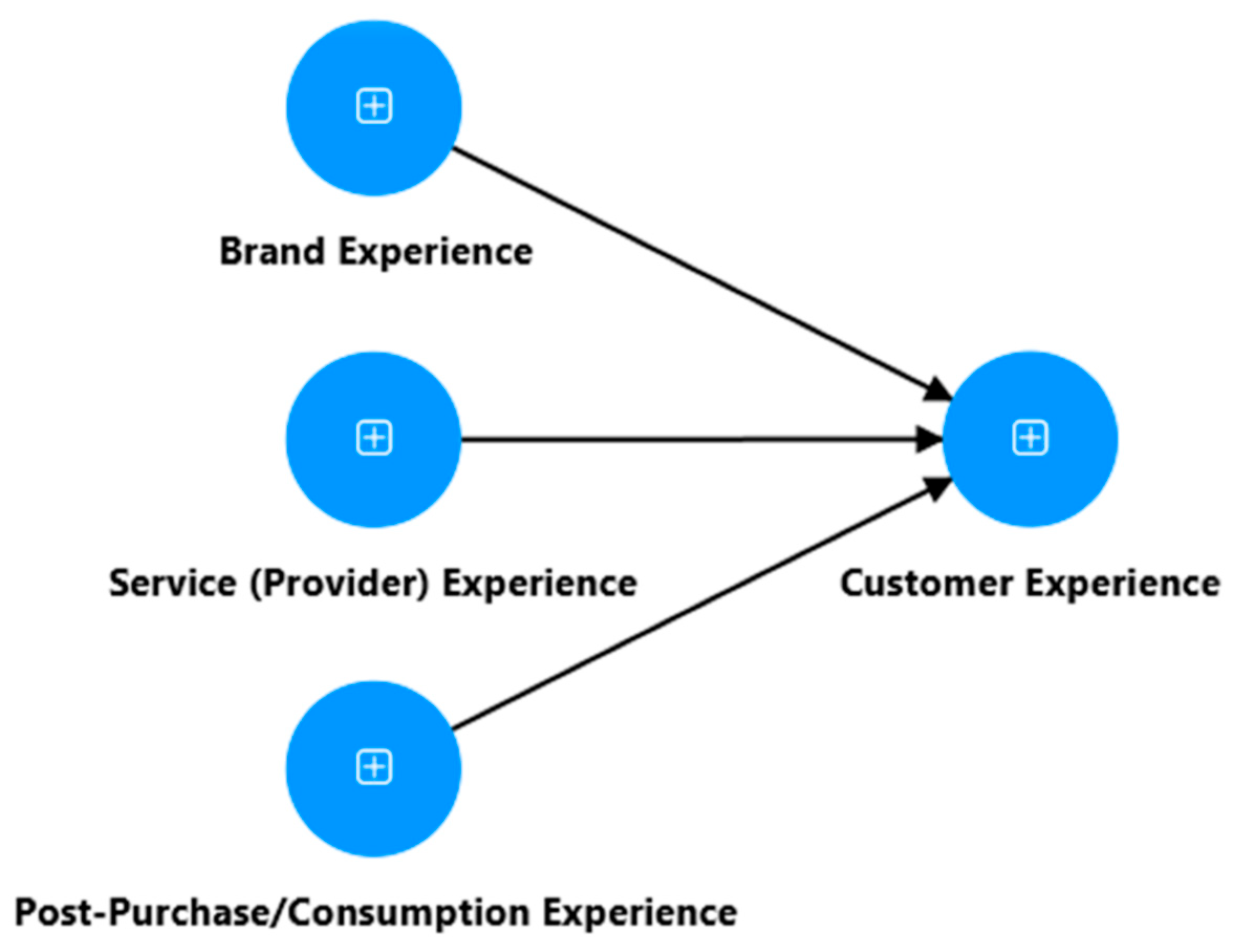
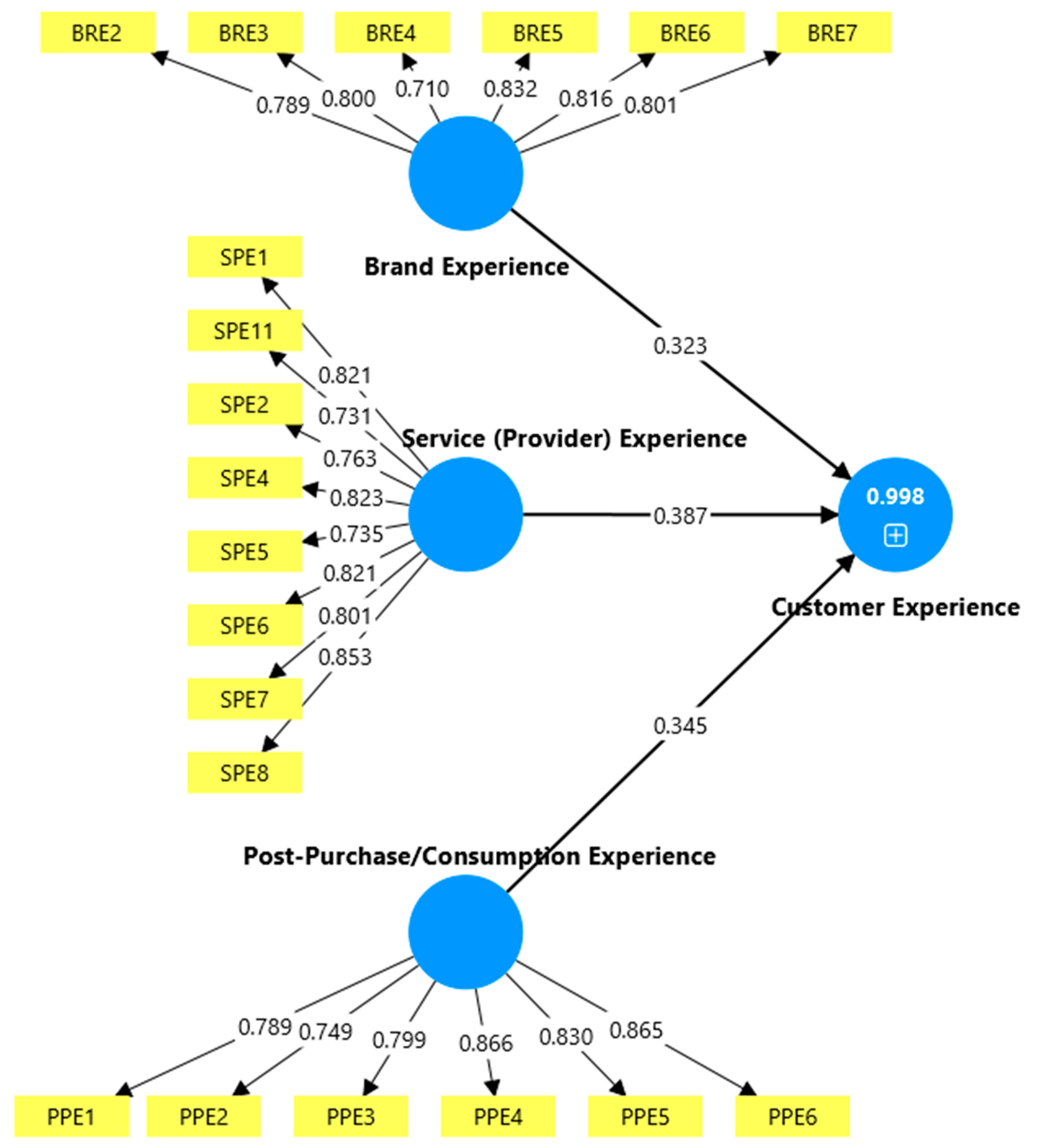
After confirming VIF values for all three independent variables and establishing the absence of multicollinearity, the analysis proceeded to assess the partial least squares analysis of the first-order model [167] presented in Appendix C, Figure A1. Additionally, the coefficient of determination (R²), which indicates the explanatory power of independent variables in a statistical model to account for the variance of the dependent variable, shows a high value R² = 0.998, which leads to the conclusion that only 0.2% of the variance in the latent variable Customer Experience is attributable to influences outside the model [167]. To eliminate issues with an overly high R² value, a stepwise approach was conducted using latent variable scores, dividing the estimation of the model into separate steps.

After applying the Partial Least Squares (PLS) method, the bootstrapping procedure was conducted. Bootstrapping can be defined as a resampling technique that, based on the available data from an initial sample, generates a large number of new samples of the same size as the original sample by randomly drawing observations with replacement [183]. In this way, each unit has an equal probability of being included in a sample, and once included, it is returned to the population from which it was drawn, allowing it to be selected multiple times, as its probability of selection remains constant throughout the resampling process.

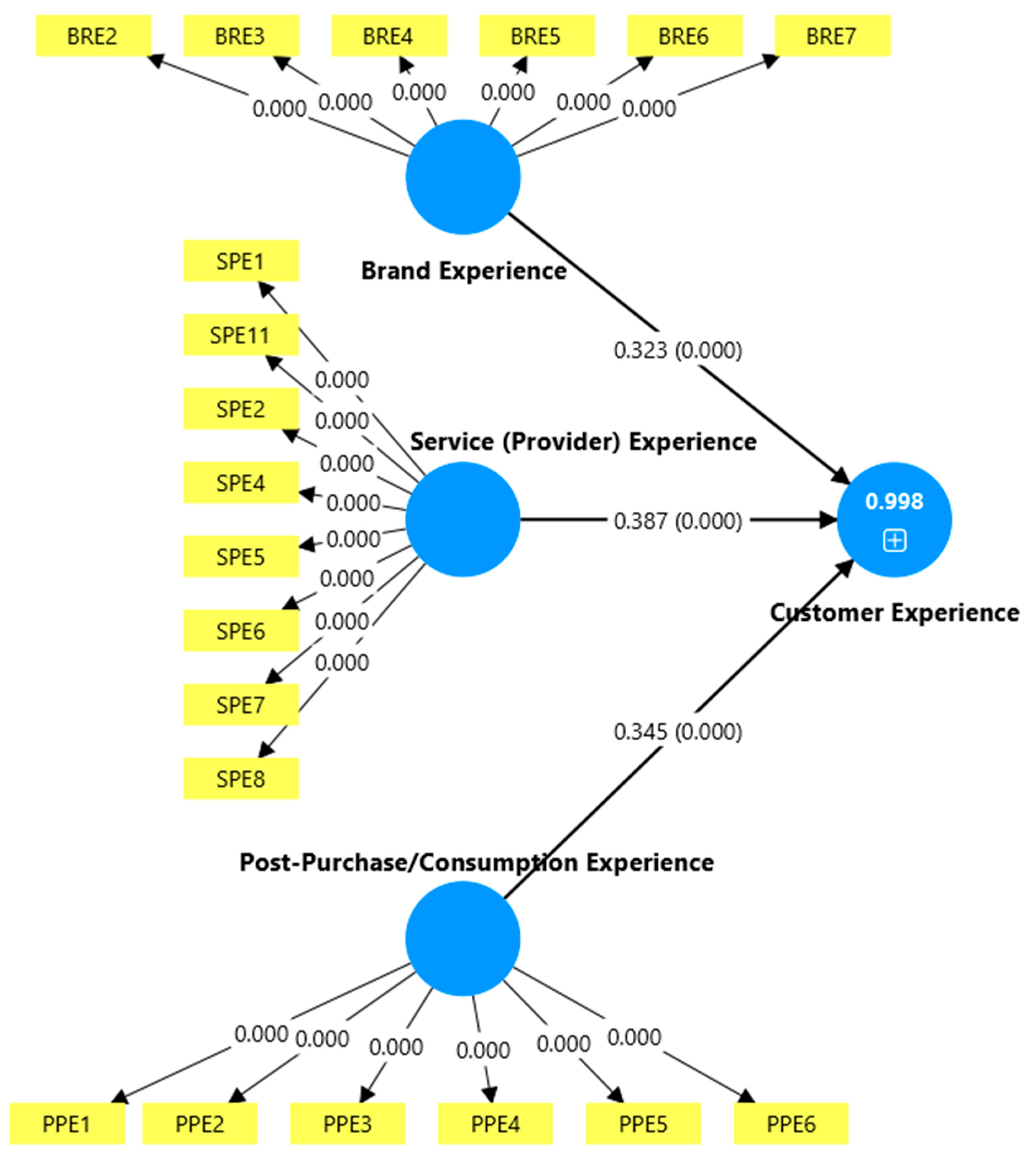
The bootstrapping results presented in Appendix C, Figure A2, determined the path coefficients, along with an assessment of the statistical significance of the retained indicators in the model and the significance of the path coefficients themselves. The evaluation of path coefficients reflects the relevance of formative constructs in the model. Since all significance parameters equal 0 (p < 0.001), it can be concluded that all path coefficients are highly statistically significant [167,184].

All three independent variables form a positive (defined by the values of β in

Table 2. The path coefficient and statistical significance of path coefficients in the inner model.

Path	β	Sample Mean	Standard Deviation	T Statistics	p Values
Brand Experience → CX	0.323	0.323	0.007	43.663	0.000
Service (Provider) Experience → CX	0.387	0.387	0.008	47.911	0.000
Post-Purchase/Consumption Experience → CX	0.345	0.345	0.008	44.921	0.000

) and highly significant (represented by p values in Table 2) relationship with Customer Experience. Thus, variable Customer Experience is formatively determined by independent variables. After establishing the direction, strength, and statistical significance of the relationships in the model, it is necessary to assess the model’s predictive power. The results of the predictive analysis for the retained parameters in the model are presented in Appendix D,

Table A5. Descriptive statistics of parameter and predictive power of first-order model.

Item	Min	Max	Mean	Standard Deviation	Q2 Predict
BRE2	1	7	4.708	1.417	0.513
BRE3	1	7	4.498	1.481	0.600
BRE4	1	7	4.906	1.579	0.409
BRE5	1	7	4.813	1.471	0.605
BRE6	1	7	4.247	1.361	0.628
BRE7	1	7	4.213	1.357	0.507
SPE2	1	7	4.990	1.430	0.545
SPE4	1	7	4.563	1.495	0.644
SPE5	1	7	4.735	1.549	0.435
SPE6	1	7	4.519	1.496	0.614
SPE7	1	7	5.073	1.420	0.562
SPE8	1	7	4.820	1.311	0.711
SPE11	1	7	4.989	1.336	0.486
PPE1	1	7	4.705	1.544	0.532
PPE2	1	7	4.266	1.394	0.586
PPE3	1	7	5.06	1.344	0.549
PPE4	1	7	4.604	1.462	0.628
PPE5	1	7	4.279	1.468	0.590
PPE6	1	7	5.080	1.267	0.707

. For each indicator, the minimum, mean, and maximum values are shown, along with the standard deviation value. The most important parameter is the predictive relevance value (Q² predict). Predictive relevance is defined as the ratio of the sum of squared prediction errors of the PLS path model to the sum of squared prediction errors of the mean benchmark model, expressed as one minus this ratio. A positive value of this parameter provides evidence that the prediction error of the PLS path model is smaller than the error produced by the most naïve benchmark criterion [185]. To evaluate the strength of predictive power, the predictive relevance values are interpreted such that any positive values above 0.35 may be considered to indicate a high level of predictive relevance of the observed effect [167]. For the indicators presented in Appendix D, Table A5, it can be concluded that they exhibit an exceptionally strong level of predictive relevance for the latent variable they form, since the predictive relevance values range from 0.409 and above.

Based on the research results, it can be concluded that Hypothesis 1, Brand Experience, Service (Provider) Experience, and Post-Purchase/Consumption Experience have a positive influence on Customer Experience, is supported.

4.3. Structural Equation Modeling of the Overall Hierarchical Model

The analysis for the overall hierarchical model was assessed using the same techniques. First, the presence of multicollinearity was assessed using the Variance Inflation Factor (VIF) for all model indicators (see Appendix B,

Table A4. Convergent and discriminant validity of the MOCE scale.

Indicator	VIF
Brand Experience	2.889
Service (Provider) Experience	3.672
Post-Purchase/Consumption Experience	3.320
SAT1	2.986
SAT2	2.519
SAT3	2.534
SAT4	3.223
SAT5	3.289
L1	3.559
L2	4.761
L3	3.870
L4	3.964
L5	2.487
WOM1	2.775
WOM2	2.894
WOM3	3.131
WOM4	3.409
WOM5	4.413

). The analysis proceeded to evaluate the outer loadings of indicators and their significance [167], as presented in Appendix E, Figure A3.

Discriminant validity is demonstrated when each measurement item correlates weakly with constructs other than the one it is theoretically associated with. Discriminant validity was tested by examining the cross-loadings of the indicators [169,186] presented in Appendix F,

Table A7. Cross-loadings of the indicators in hierarchical model.

Indicator	Customer Experience	Customer Satisfaction	Behavioral Loyalty Intensions	Word-of-Mouth
BRE	0.909	0.790	0.660	0.538
SPE	0.938	0.866	0.728	0.585
PPE	0.929	0.861	0.734	0.603
SAT1	0.773	0.872	0.745	0.601
SAT2	0.793	0.857	0.655	0.519
SAT3	0.793	0.856	0.710	0.510
SAT4	0.829	0.894	0.681	0.579
SAT5	0.771	0.882	0.711	0.577
L1	0.689	0.736	0.898	0.668
L2	0.735	0.776	0.930	0.699
L3	0.673	0.715	0.900	0.734
L4	0.692	0.720	0.911	0.636
L5	0.640	0.644	0.843	0.613
WOM1	0.512	0.520	0.624	0.863
WOM2	0.516	0.520	0.633	0.871
WOM3	0.562	0.563	0.623	0.887
WOM4	0.578	0.613	0.714	0.894
WOM5	0.592	0.613	0.720	0.924

. The highlighted items represent the factor loadings for each construct, while the cross-loadings are reported in the unshaded cells. It can be observed that the cross-loadings for each construct are low, which indicates good discriminant validity. For the Customer Experience construct, the factor scores of the latent variables were considered as indicators, and these loadings correlate more strongly with the construct they define than with the other constructs in the model.

Discriminant validity was also assessed using the Heterotrait–Monotrait (HTMT) ratio of correlations. This measure assesses how well the constructs in the model differ from one another, ensuring that each captures a distinct aspect of the phenomenon under investigation. An HTMT value below 0.90 generally indicates good discriminant validity, meaning that the constructs are sufficiently distinct to be treated as separate [167,186]. The results of the HTMT analysis are presented in Appendix G,

Table A8. Heterotrait–Monotrait (HTMT) ratio of correlations of hierarchical model.

Indicator	L	CX	SAT	WOM	Segment	Gender	Region	Gender x CX	Segment x CX	Region x CX
L
CX	0.824
SAT	0.862	0.876
WOM	0.798	0.672	0.687
segment	0.020	0.007	0.019	0.091
gender	0.168	0.171	0.138	0.176	0.161
region	0.029	0.018	0.015	0.016	0.028	0.074
gender x CX	0.567	0.788	0.735	0.499	0.002	0.087	0.011
segment x CX	0.425	0.559	0.530	0.343	0.005	0.078	0.014	0.340
region x CX	0.104	0.100	0.091	0.104	0.009	0.003	0.352	0.030	0.006

. The results presented in Appendix F and G, based on two different analyses, confirm that the criterion of discriminant validity of the model has been satisfied.

After establishing discriminant validity, a metric invariance test was conducted to examine the potential moderating influence of categorical variables. The goal is to statistically confirm that the instrument measures the same underlying concept consistently across groups, ensuring that any observed differences in scores reflect true differences in the construct rather than measurement bias, thereby making comparisons valid.

Configural invariance (Model 1) was tested for gender, with the factor structure free across groups. Model 1 exhibited a good fit (Χ² (df) = 677.188(258), CFI = 0.959, RMSEA = 0.051), confirming that the same pattern of latent factors existed for both men and women. Next, a metric invariance (Model 2) was tested by constraining the factor loadings to be equal across groups. Compared to the configural model, the metric model (Model 2) did not show a significant decrease in model fit: (Delta CFI = −0.001) with p = 0.124. Therefore, metric invariance was established, indicating that the items contributed to the constructs to a similar extent for both men and women.

For customer segments, Model 1 exhibited good fit (Χ² (df) = 719.161(258), CFI = 0.956, RMSEA = 0.054), confirming that the same pattern of latent factors existed for both individual and corporate segments of customers. The metric model (Model 2) did not show a significant decrease in model fit: (Delta CFI = 0) with p = 0.364. Therefore, metric invariance was established, indicating that the items contributed to the constructs to a similar extent for both individual and corporate customer segments.

For regions Model 1 showed good fit (Χ² (df) = 672.333(258), CFI = 0.955, RMSEA = 0.052), confirming that the same pattern of latent factors existed for both Belgrade and Vojvodina region respondents. The metric model (Model 2) did not exhibit a significant decrease in model fit: (Delta CFI = 0) with p = 0.167. Therefore, metric invariance was established, indicating that the items contributed to the constructs to a similar extent for both Belgrade and Vojvodina region respondents.

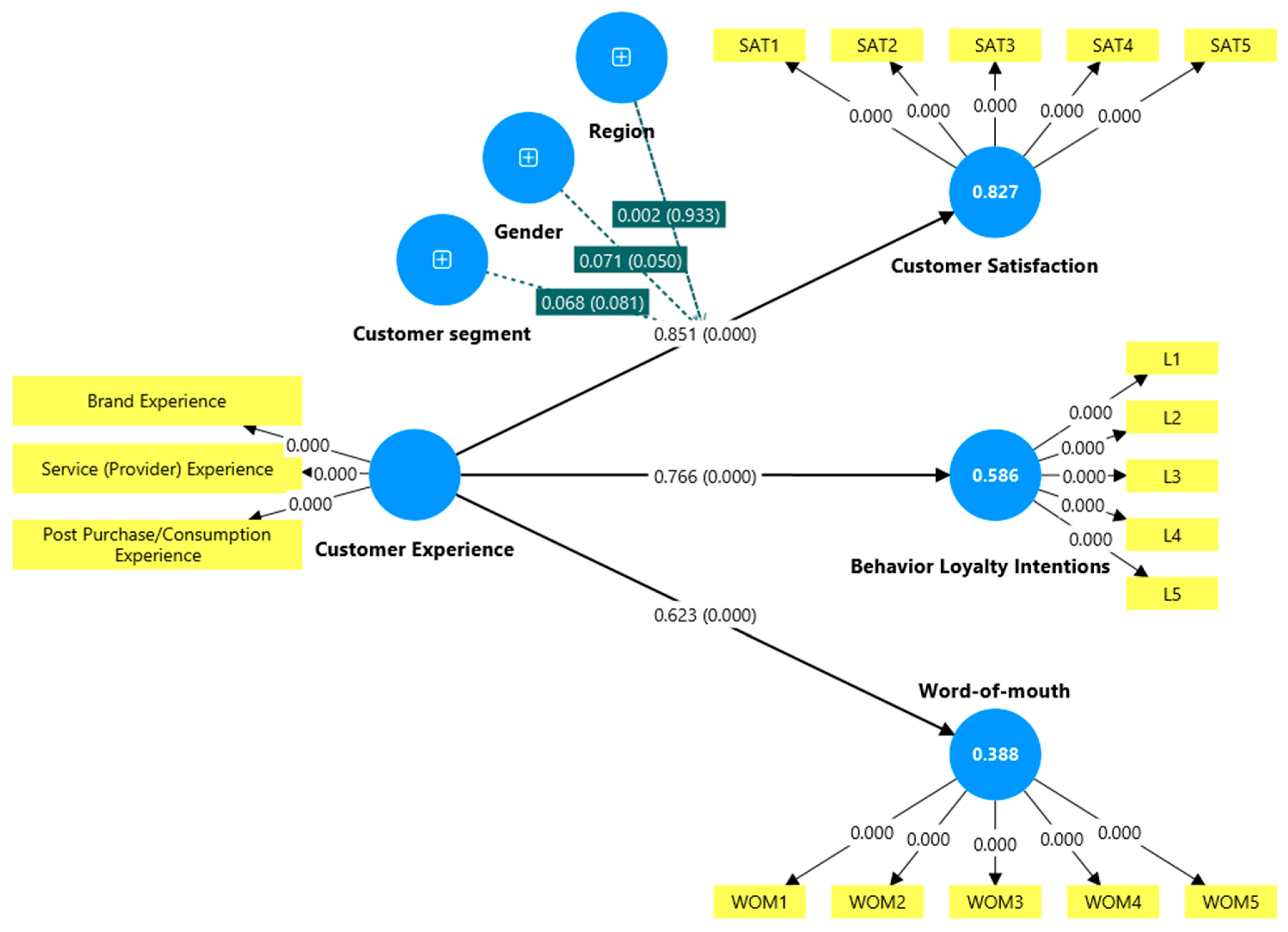
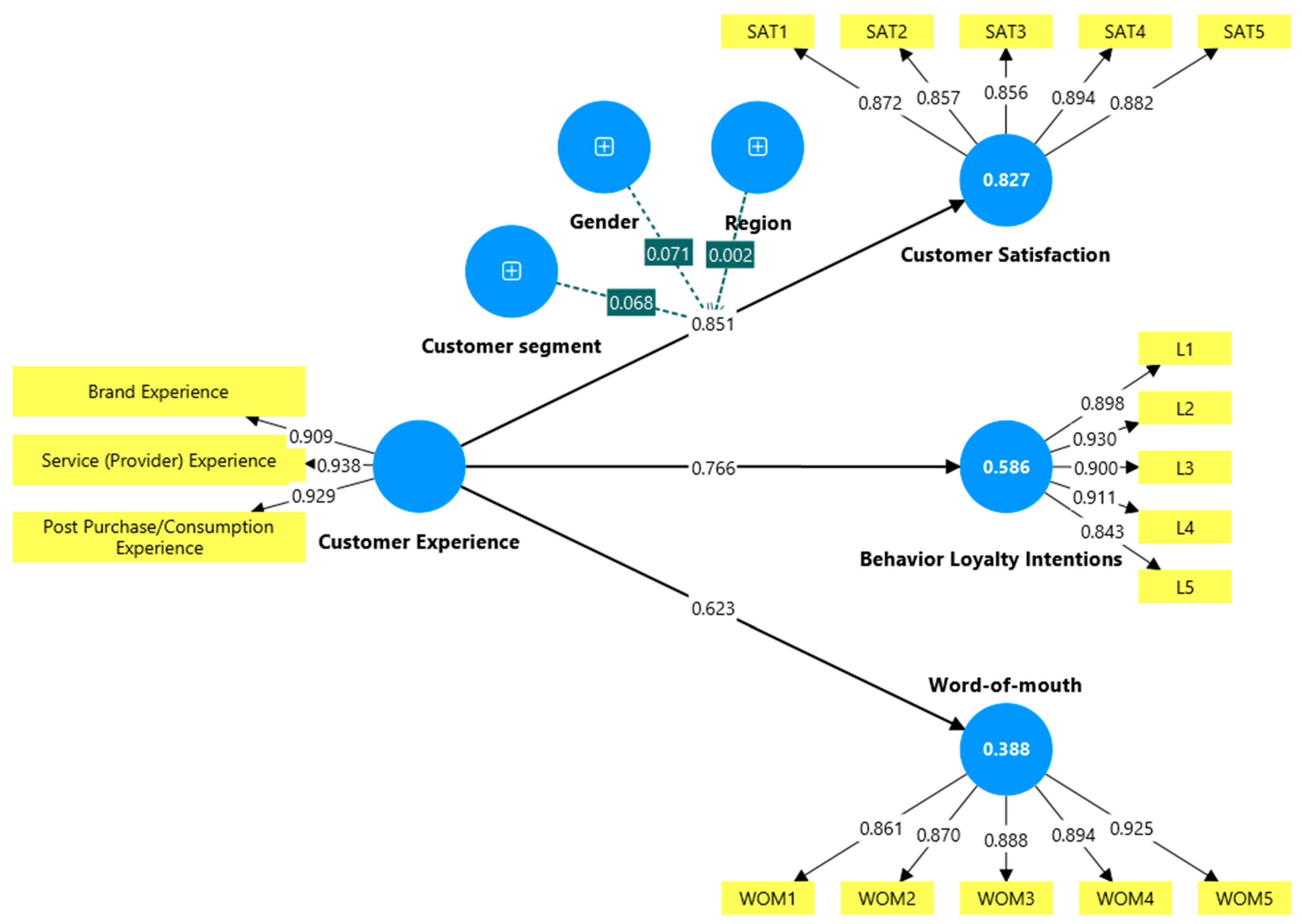
The results of bootstrapping analysis for the hierarchical model are presented in

Table 3. The path coefficient and statistical significance of the path coefficients in the overall hierarchical model.

Path	β	Sample Mean	Standard Deviation	T Statistics	p Values
CX → Customer Satisfaction	0.851	0.851	0.026	32.191	0.000
CX → Behavioral Loyalty Intensions	0.766	0.766	0.026	29.463	0.000
CX → Word-of-mouth	0.623	0.623	0.027	23.372	0.000
customer segment → Customer Satisfaction	−0.013	−0.014	0.040	0.334	0.738
customer segment x CX → Customer Satisfaction	0.068	0.070	0.039	1.744	0.081
gender → Customer Satisfaction	−0.03	−0.031	0.037	0.821	0.412
gender x CX → Customer Satisfaction	0.071	0.070	0.036	1.964	0.050
region affiliation → Customer Satisfaction	0.009	0.007	0.020	0.436	0.663
region affiliation x CX → Customer Satisfaction	0.002	0.003	0.022	0.084	0.933

and Figure 3.

After the analysis presented in Table 3, it is confirmed that there is a positive and statistically significant relationship between the variable Customer Experience and the variable Customer Satisfaction as an aspect of the marketing outcomes of customer experience. The path coefficient of this relationship (β = 0.851) indicates a positive relationship, while the corresponding p-value (p < 0.001) demonstrates a high level of statistical significance. The interpretation of the results confirms the theoretical assumption that customers who perceive better CX (in terms of brand, service, and post-purchase activities) also demonstrate higher levels of customer satisfaction [56,58].

Based on the research results, it can be concluded that Hypothesis 2, Customer Experience has a positive influence on Customer Satisfaction, is supported.

Table 3 presents results that confirm a positive and statistically significant relationship between the variable Customer Experience and the variable Behavior Loyalty Intentions as another aspect of the marketing outcomes of customer experience. The path coefficient (β = 0.766) indicates a positive relationship, while the corresponding p-value (p < 0.001) demonstrates a high level of statistical significance. The interpretation of the results supports the theoretical proposition that customers who perceive better customer experience (in terms of brand, service, and post-purchase activities) are more likely to be loyal [134,187].

Based on the research results, it can be concluded that Hypothesis 3, Customer Experience has a positive influence on Behavior Loyalty Intentions, is supported.

Finally, the results presented in Table 3 show a positive and statistically significant relationship between Customer Experience and Word-of-Mouth as a marketing outcome of customer experience. The path coefficient (β = 0.623) is positive, and the corresponding p-value indicates high statistical significance (p < 0.001). This supports the theoretical proposition that customers who perceive a better customer experience (in terms of brand, service, and post-purchase activities) are more likely to engage in positive WOM, thereby recommending the service or company to others [145,149].

Based on the research results, it can be concluded that Hypothesis 4, Customer Experience has a positive influence on Word-of-Mouth, is supported.

After establishing the direction, strength, and statistical significance of the relationships in the model, it is necessary to evaluate the predictive power of the model. The results of the predictive analysis for the retained parameters in the hierarchical model are presented in Appendix D,

Table A6. Descriptive statistics of parameter and predictive power of hierarchical model.

Item	Min	Max	Mean	Standard Deviation	Q2 Predict
BRE	1	7
SPE	1	7
PPE	1	7
SAT1	1	7	4.494	1.454	0.596
SAT2	1	7	4.503	1.499	0.626
SAT3	1	7	5.088	1.318	0.624
SAT4	1	7	4.446	1.431	0.684
SAT5	1	7	4.471	1.383	0.590
L1	1	7	4.570	1.385	0.472
L2	1	7	4.252	1.450	0.536
L3	1	7	4.779	1.303	0.450
L4	1	7	4.568	1.389	0.476
L5	1	7	4.600	1.296	0.408
WOM1	1	7	3.707	1.513	0.259
WOM2	1	7	3.205	1.719	0.262
WOM3	1	7	3.608	1.695	0.313
WOM4	1	7	3.602	1.807	0.331
WOM5	1	7	3.747	1.620	0.347

. For each indicator, the minimum, mean, and maximum values are reported, along with the standard deviation value. The most important parameter is the predictive relevance value (Q² predict), where a positive value provides evidence that the prediction error of the PLS path model is smaller than the error generated by the most naïve benchmark criterion [185].

To assess the strength of predictive power, the values of predictive relevance are interpreted such that any positive values above 0.35 can be considered to represent a strong degree of predictive significance for the observed effect [167]. For the indicators analyzed, it can be concluded that they demonstrate an exceptionally high level of predictive significance for the latent variable they form. The lowest predictive power was observed for the indicators of the variable WOM, whose predictive parameters fall within the interval of 0.15 to 0.35, thereby reflecting moderate predictive power (Appendix D, Table A6).

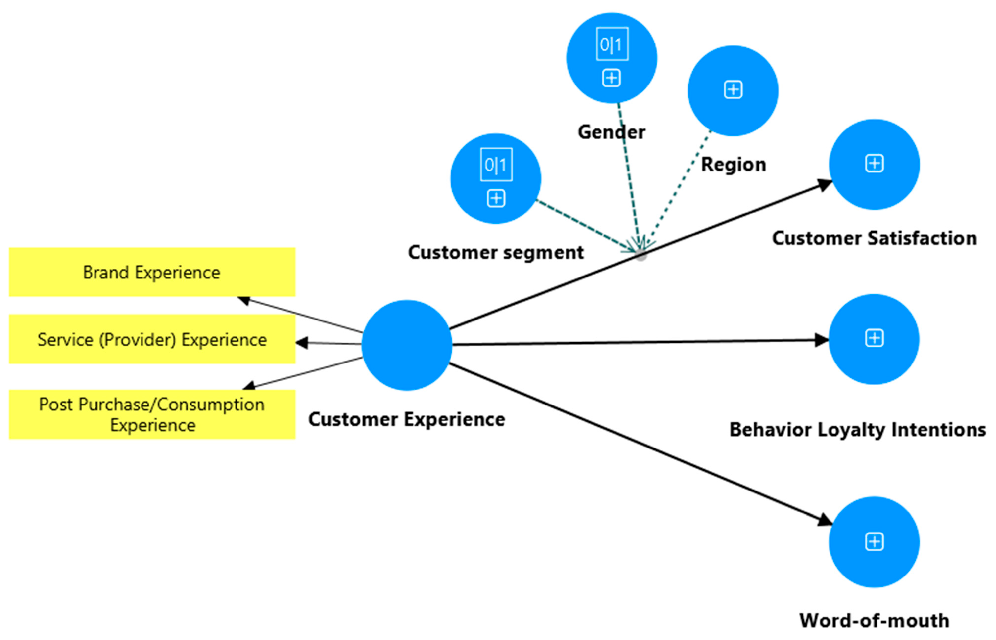
Within the scope of this study, the potential moderating influence of variables on the relationship between customer experience and the aspects of marketing outcomes of customer experience was examined [167,188,189].

The results of testing the structural relationships of the model provide insight into the existence of a directional effect of independent variables, such as customer segment, respondents’ gender, or regional affiliation of respondents, on the relationship between customer experience and the aspects of marketing outcomes related to customer experience.

The assessment of the directional influence of independent variables was conducted stepwise, based on potential moderating effects on the observed relationships in the model, and is presented in Table 3. The results suggest that the existence of a positive directional impact of the variable Customer Segment on the relationship between Customer Experience and Customer Satisfaction is debatable. The path coefficient (β = 0.068) indicates a positive directional effect, which can be interpreted as follows: the relationship between Customer Experience and Customer Satisfaction is strengthened by 0.068 units with each standard deviation of the variable Customer Segment. Thus, the variable Customer Segment may be considered to have a strengthening effect.

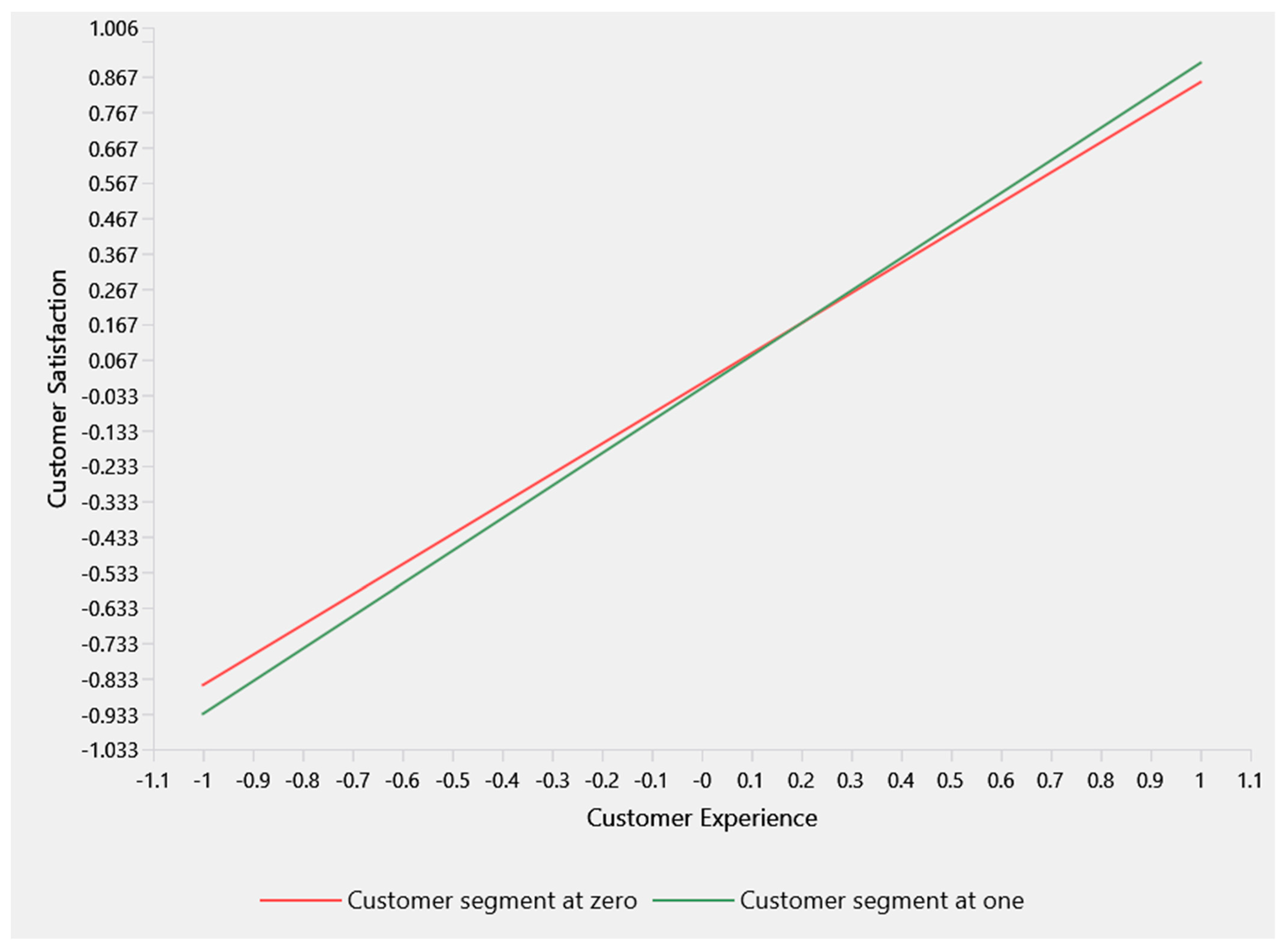
For the conclusion to be meaningful, it is also necessary to consider the p-value (p = 0.81), indicating exceptionally weak statistical significance of the parameter (Table 3). Although this may not be sufficient evidence of statistical significance, it does indicate a trend (as p < 0.1). To gain a better understanding of the potentially moderating effect of the variable Customer Segment, which divides the sample into sub-samples of individual customers and commercial customers, Figure 4 may be helpful.

Figure 4 illustrates the interaction of variables within the moderating relationship. On the abscissa, the variable Customer Experience is presented using centered values, which also highlight negative values, thereby distinguishing low, medium, and high levels of Customer Experience. On the ordinate, the variable Customer Satisfaction is displayed, likewise using centered values, allowing for a clear identification of low, medium, and high levels of satisfaction.

The lines, presented in two colors, depict the relationship of different segments to the connection between the specified variables, for which a significant directional effect of the two subsamples can be established. Respondents from the commercial segment (represented by the green line) are portrayed with a steeper slope line compared to respondents from the individual customer segment (represented by the red line).

In summary, the conclusion is that a high level of satisfaction may be expected not only as a result of a high level of customer experience, but also as influenced by the customer segment to which they belong. Put differently, when customer experience is at a low level, and respondents are individual customers, higher customer satisfaction is expected, as a noted trend.

Based on the research results, it can be concluded that Hypothesis 5, Customer segment has a moderating effect on the relationship between customer experience and customer satisfaction, is not supported.

The analysis of path coefficients presented in Table 3 enables us to conclude the moderating effect of the variable Gender on the observed relationships within the model. The value of the path coefficient (β = 0.071) confirms a positive directional impact of the variable Gender on the relationship between Customer Experience and Customer Satisfaction, which can be interpreted as follows: the relationship between Customer Experience and Customer Satisfaction strengthens by 0.071 units with each standard deviation in the variable Gender. Consequently, the variable Gender may be regarded as an enhancing factor.

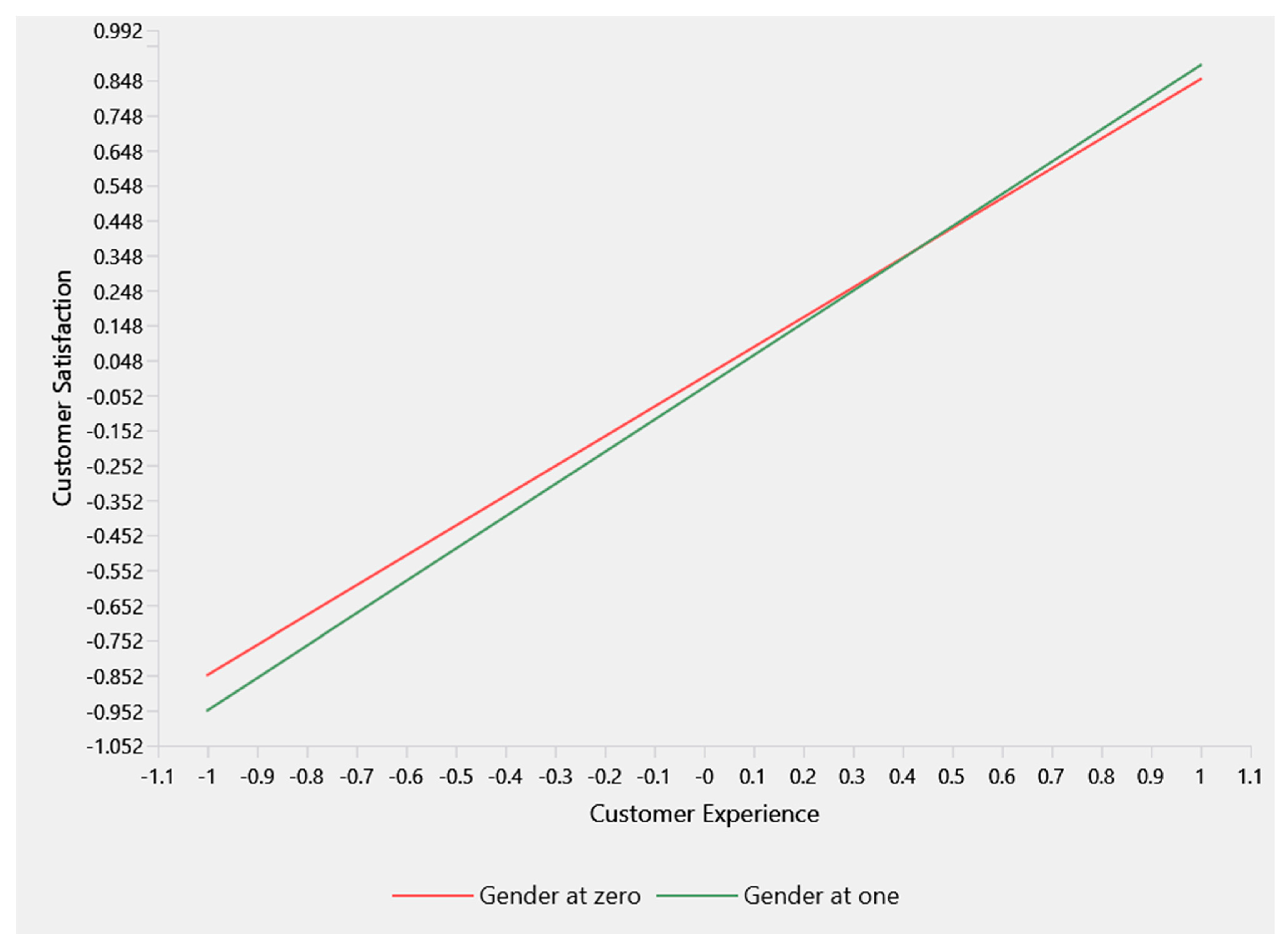
To ensure the conclusion is meaningful, it is also necessary to consider the p-value, which indicates the statistical significance of the parameter. For this effect (Table 3), the relationship is statistically significant at the p = 0.05 level, which is considered sufficient evidence of statistical significance. To better understand the moderating effect of the variable Gender, which divides the sample into subsamples of female and male respondents, a graphical representation may be helpful, as shown in Figure 5.

Figure 5 illustrates the interaction of variables within the moderating relationship. The lines depict the relationship between different genders with respect to the specified variables, for which a statistically significant directional effect can be identified in the two subsamples. Respondents of male gender (represented by the green line) are portrayed with a steeper slope line compared to respondents of female gender (represented by the red line).

The conclusion is that a high level of satisfaction can be expected not only from a high level of customer experience, but also because of a particular gender. When customer experience is at a low level, female respondents tend to contribute to higher customer satisfaction, whereas male respondents may report lower customer satisfaction.

Based on the research results, it can be concluded that Hypothesis 6, Gender has a moderating effect on the relationship between customer experience and customer satisfaction, is supported.

Based on the results of the analysis in Table 3, it is possible to conclude that the variable Region has a moderating effect on the observed relationships in the model. The value of the path coefficient (β = 0.002) barely establishes a positive and extremely weak relationship. The p-value = 0.933, indicating that the regional affiliation of respondents does not significantly influence the relationship between Customer Experience and Customer Satisfaction. Therefore, there is no need to perform a slope analysis graphically. Although the variable regional affiliation of respondents divides the sample into subsamples for Belgrade, Vojvodina, and Other, no influence could be determined in the specified model.

Based on the research results, regional affiliation does not moderate the relationship between customer experience and customer satisfaction. Thus, Hypothesis 7 is not supported.

Potential moderating effects of the chosen variables were not found to indicate even a trend in the remaining structural relationships between customer experience and behavioral loyalty intentions, nor between customer experience and word-of-mouth.

Following the statistical confirmation of the direction, strength, and statistically significant effects of the variables, the discriminant validity of the final model, which includes all retained relationships, was tested. The results of the HTMT analysis are presented in Appendix G, Table A8. All values support the previously drawn conclusion based on the results measuring correlations presented in Appendix F, Table A7. The conducted analysis indicates satisfactory discriminant validity, meaning that the constructs are sufficiently distinct and can be regarded as separate [167].

Empirical evidence shows that gender influences how trust develops in mobile banking, with factors like perceived security, ease of use, and service quality affecting men and women differently. This suggests that males and females rely on different cognitive and emotional processes when building trust in digital financial services [190]. Customer experience alone doesn’t predict trust outcomes uniformly; instead, gender shapes both the strength and direction of these relationships, indicating its role as a crucial moderator, not just a control variable. These insights are especially relevant for banking systems powered by Industry 4.0 and Industry 5.0, where human–technology interactions and perceived risks are key to shaping user experience.

Additional evidence supports the idea that consumer demographics, such as gender, influence how customer experience affects satisfaction, word-of-mouth intentions, and loyalty [191]. The effect of customer experience on marketing outcomes differs notably between men and women, especially regarding relationships like loyalty and WOM, indicating that gender not only influences how customers evaluate their experience but also shapes their behavioral intentions and how they communicate after purchase.

Prior empirical evidence in the extant literature, along with the findings reported in this study, emphasize that the inclusion of demographic moderating variables significantly enhances the accuracy and practical usefulness of customer experience (CX) models. Demographic moderators, such as gender, customer segments, or regions, enable researchers to capture systematic differences in how distinct customer groups perceive service encounters and translate experiential evaluations into attitudinal and behavioral outcomes.

From both methodological and managerial perspectives, incorporating demographic moderating effects enhances model validity and relevance. By acknowledging demographic differences, CX models offer more precise diagnostic value and support the development of targeted, human-centric, and context-sensitive customer experience strategies that are consistent with a systems-oriented view of service design and the principles of Industry 5.0.

5. Discussion

This research provides a deeper understanding of a holistic conceptual model that represents customer experience in the banking sector. Furthermore, the results may shed light on possibilities for developing rigorous mechanisms for ongoing monitoring and evaluation of CX throughout the customer journey, which is in line with studies evidencing that higher customer satisfaction yields business growth [47,48]. Employing the EXQ scale in the research enabled capturing all three stages of the customer journey: pre-purchase (BRE dimension), purchase (SPE dimension), and after purchase (PPE dimension).

Service Provider Experience was identified as the most important customer experience influencing factor in the model (Appendix, Figure A1 and Figure A3), with purchase experience as the most important journey stage. Furthermore, the most influential aspects of the SPE dimension driving CX are the quality of customer service and the perceived flexibility of the bank providing service (Appendix A, Table A1). Service experience, encompassing both interpersonal interactions and digital touchpoints, significantly shapes customer satisfaction and loyalty. Consistent with service-dominant logic, value is co-created through ongoing interactions among customers, employees, and technological systems, making banking experience a hybrid of relational and digital elements [192]. Prior studies confirm the importance of customer–employee rapport [91] and emotional responses [193], while recent evidence shows that FinTech capabilities [194] and AI-driven personalization [195] strengthen the links between satisfaction and retention. Collectively, these findings underscore that human–technology integration, aligned with Industry 5.0 principles, enhances relational outcomes and fosters long-term loyalty in banking.

Post-Purchase Experience was identified as the second most important CX influencing factor in the model, underscoring the importance of delivering CX after the service stage of the customer journey. The most important aspects of PPE were determined to be long-term care dedication and the level of perceived happiness with the service provided (Appendix A, Table A1). The post-purchase stage is critical for reinforcing or eroding customer trust over time. In line with holistic customer journey models [19,110], these findings underscore the importance of managing post-purchase experience as a continuous, relationship-building process rather than as isolated touchpoints.

Brand Experience, as the third most important influencing factor on CX in a model, is mostly represented by first-line employees who embody the brand accordingly (Appendix A, Table A1), leading to the conclusion that the pre-purchase customer journey stage is the least important for creating customer experience. In line with Berry’s service brand equity framework [196], brand cues reduce perceived risk and shape expectations, a function especially salient in transitional economies such as Serbia, where institutional trust remains fragile. Prior research confirms that image and reputation drive loyalty in financial services, positioning brand experience as a relational asset rather than a purely symbolic construct [197,198]. Recent evidence further shows that digital quality and socially responsible online cues strengthen satisfaction and loyalty, reinforcing the central role of brand experience within the EXQ framework amid digital and institutional transformation [198,199].

The holistic model presented in this study, which scrutinizes relationships between CX and marketing outcomes, provides evidence of a positive, statistically significant influence of CX on all marketing outcomes. The study’s findings indicate that CX is the antecedent construct for all marketing outcomes.

A positive and significant relationship between CX and Customer Satisfaction was proven to be the strongest in the model (the model accounts for almost 83% of the variance in customer satisfaction (Figure 3) and has the greatest predictive power (Appendix D, Table A6) for the SAT aspect), as has been suggested by Maklan and Klaus [24,141], Roy [51], Sharma et al. [200], and others.

Furthermore, in this research, it was found that the relationship between CX and Behavioral Loyalty Intentions is positive and significant, acknowledging Zeithaml et al. [72,93] and Ranaweera and Prabhu [144]. Additionally, it was found that the relationship between CX and WOM is positive and significant, confirming research by Brown et al. [149]. These results suggest that CX should precede all marketing outcomes. The preceding statement aligns with a significant number of studies that link CX to loyalty and WOM, while contradicting Pires et al. [201] that suggests that CX should only precede customer satisfaction.

The results on the moderating effects of customer demographics are informative and add to the literature, particularly regarding gender-specific influences on CX and marketing outcomes. Gender was found to significantly amplify the positive relationship between Customer Experience and Customer Satisfaction. The findings suggest that satisfaction is more affected by perceived improvements in customer experience among male respondents, while women tend to report relatively stable satisfaction levels even at lower levels of customer experience.

Conversely, the moderating role of the customer segment (individual vs. commercial customers) on the significant relationships in the model was not statistically significant, though a trend suggesting that commercial clients might amplify the positive relationship between Customer Experience and Customer Satisfaction was observed. The regional affiliation of respondents did not have a meaningful impact on significant relationships explained by the model, reflecting the increasing uniformity of banking services across Serbia.

6. Conclusions

Industry 5.0 should be understood as a progression of Industry 4.0, building on its digital and efficiency-driven foundations while shifting the focus toward human-centricity, sustainability, and resilience. Accordingly, customer experience research must extend beyond efficiency and convenience to incorporate relational dimensions. From a marketing perspective, this reorientation positions customer experience as a strategic asset. Conceptualized through multidimensional frameworks such as EXQ, customer experience quality serves as a key mechanism linking Industry 5.0 transformation with satisfaction, loyalty, and positive word of mouth.

6.1. Theoretical Implications

The contributions to theory are fourfold. First, the results of this study advance understanding of the mechanisms by which customer experience influences marketing outcomes, thereby building on the initial work of Klaus and Maklan [24,141]. The study adapted and validated a measurement tool tailored to the specific characteristics of an emerging economy, thereby extending the field of EXQ application and enabling cross-context comparison.

Second, the application of the EXQ scale in this study enabled a comprehensive and process-oriented assessment of customer experience by systematically capturing all three critical stages of the customer journey. This multidimensional operationalization is particularly important, as customer value creation in contemporary service systems unfolds cumulatively across touchpoints rather than at isolated transactional moments. The study developed a measurement tool tailored to the specific characteristics of an emerging economy, thereby improving the reliability and relevance of the results.

Third, this study aims to clarify the factors influencing CX and assess its impact on marketing outcomes in the Serbian banking sector. The findings show strong positive links between CX and marketing outcomes: customer satisfaction, behavioral loyalty intentions, and word-of-mouth. This positions CX as a key predictor of marketing success in banking, in line with mainstream CX literature.

Fourth, building on the baseline model of the impact of customer experience on marketing outcomes, as predominantly represented in the established literature, this study advances the conceptual framework by incorporating gender as a moderating variable. By empirically demonstrating the conditional nature of the CX–marketing outcome relationship, the findings highlight that customer experience effects are not universally homogeneous but may vary across demographic segments. Consequently, the results underscore the importance of adopting a gender-sensitive perspective in modeling and managing customer experience.

6.2. Practical Implications

This study contextualizes customer experience within a post-transition socio-economic context, shaped by path dependency, institutional discontinuities, and the history of rapid foreign-owned bank penetration. In contrast to the legacy of limited competition and weak customer orientation, customer experience in the contemporary banking sector, aligned with Industry 5.0 principles, emerges as a strategic determinant of trust, cocreation, and long-term performance. By extending experience quality research beyond mature Western markets, the findings demonstrate that in transitional economies, customer experience functions as a mechanism for reducing perceived risk and strengthening relational capital. Practically, banks should adopt a holistic, human-centric, and journey-oriented approach that integrates technological efficiency with trust-building practices, while policymakers should reinforce regulatory frameworks that enhance transparency and consumer confidence.

From a managerial perspective, bank management’s strategic orientation should focus on strengthening the service provider experience, as empirical findings indicate that this element exerts the greatest influence on the customer journey. Among the dimensions of the service provider experience, perceived service quality emerged as the most significant determinant. Given the banking sector’s advanced level of digitalization and the evolving Industry 5.0 paradigm, bank management must place greater emphasis on precise, timely measurement of service quality and the systematic implementation of corrective measures to maintain and enhance service performance standards. Furthermore, perceived flexibility in service delivery was identified as a second critical factor within the service provider experience construct. To sustain competitiveness in increasingly dynamic, customer-centric markets, banks should formulate agile strategies tailored to customers’ specific requirements, thereby aligning operational processes with the personalized value-creation principles characteristic of Industry 5.0.

Considering the overall customer experience with banking services, the findings demonstrate that it is a primary driver not only of customer satisfaction but also of increased loyalty and positive word of mouth. This indicates that customer experience functions as a central integrative construct linking service encounters to key marketing performance outcomes. By systematically managing and optimizing the end-to-end customer experience, bank management can simultaneously influence three critical positive marketing outcomes, thereby enhancing both relational capital and long-term competitive positioning.

A particularly relevant managerial implication of this study is the confirmed moderating effect of gender on the statistically significant relationship between customer experience and customer satisfaction. This finding suggests that the impact of customer experience on satisfaction is not uniform across customer groups, requiring bank management to design differentiated strategies aligned with gender-based segmentation. In addition, the results indicate an evident trend in how business and individual customers shape the relationship between customer experience and satisfaction. Accordingly, bank management should develop distinct strategic approaches and service design frameworks for commercial and individual customers to more effectively manage and enhance satisfaction levels across heterogeneous customer segments.

Furthermore, the adaptation and validation of the EXQ scale confirmed its cross-contextual applicability within the Serbian banking sector. This finding indicates that local clients’ expectations regarding service quality are largely aligned with those of customers in the banks’ countries of origin. From a managerial standpoint, this suggests that international banks operating in Serbia can leverage standardized customer experience management frameworks while making context-sensitive adjustments, thereby achieving efficiency through strategic alignment without compromising local market responsiveness.

6.3. Limitations and Further Research

This study is subject to several limitations. First, the empirical context is limited to Serbia, which may constrain the generalizability of the findings to other transitional or developed economies. Second, the age structure of the sample is skewed toward respondents aged 25–44, a digitally proficient and economically active cohort, potentially underrepresenting younger and older customer segments and influencing the observed structural relationships. Third, the cross-sectional design captures perceptions at a single point in time and does not account for dynamic changes in customer experience. Additionally, while gender was confirmed as a significant moderator, other relevant variables, such as income, digital literacy, and generational cohort, were not incorporated.

Future research should extend the model by incorporating mediating mechanisms among marketing outcomes and including additional moderating variables to better capture heterogeneity across customer segments. Comparative cross-country studies, particularly between transitional and developed economies, would provide deeper insight into institutional and cultural contingencies shaping customer experience. Longitudinal designs are recommended to examine the evolving nature of customer experience amid digital transformation and the transition toward Industry 5.0. Furthermore, expanding the application of the EXQ framework beyond banking to other service sectors, such as retail, healthcare, education, tourism, and digital services, would contribute to developing a more comprehensive, context-sensitive theoretical model of customer experience.

In summary, the present study substantiates that customer experience is a pivotal determinant of marketing outcomes in the banking sector rather than a peripheral variable. The findings offer robust empirical support for managerial investments in customer experience enhancement initiatives and unveil detailed insights into demographic and segmentation disparities. Future research avenues include integrating longitudinal data, conducting comparative analyses between Serbia and other emerging economies, and exploring additional moderating factors, such as income levels, digital literacy, and generational cohorts.