
Spatiotemporal Changes and Driving Forces of the Ecosystem Service Sustainability in Typical Watertown Region of China from 2000 to 2020

 ,
,  ,
,
Abstract
1. Introduction
2. Materials and Methods
2.1. Study Area
2.2. Data Sources
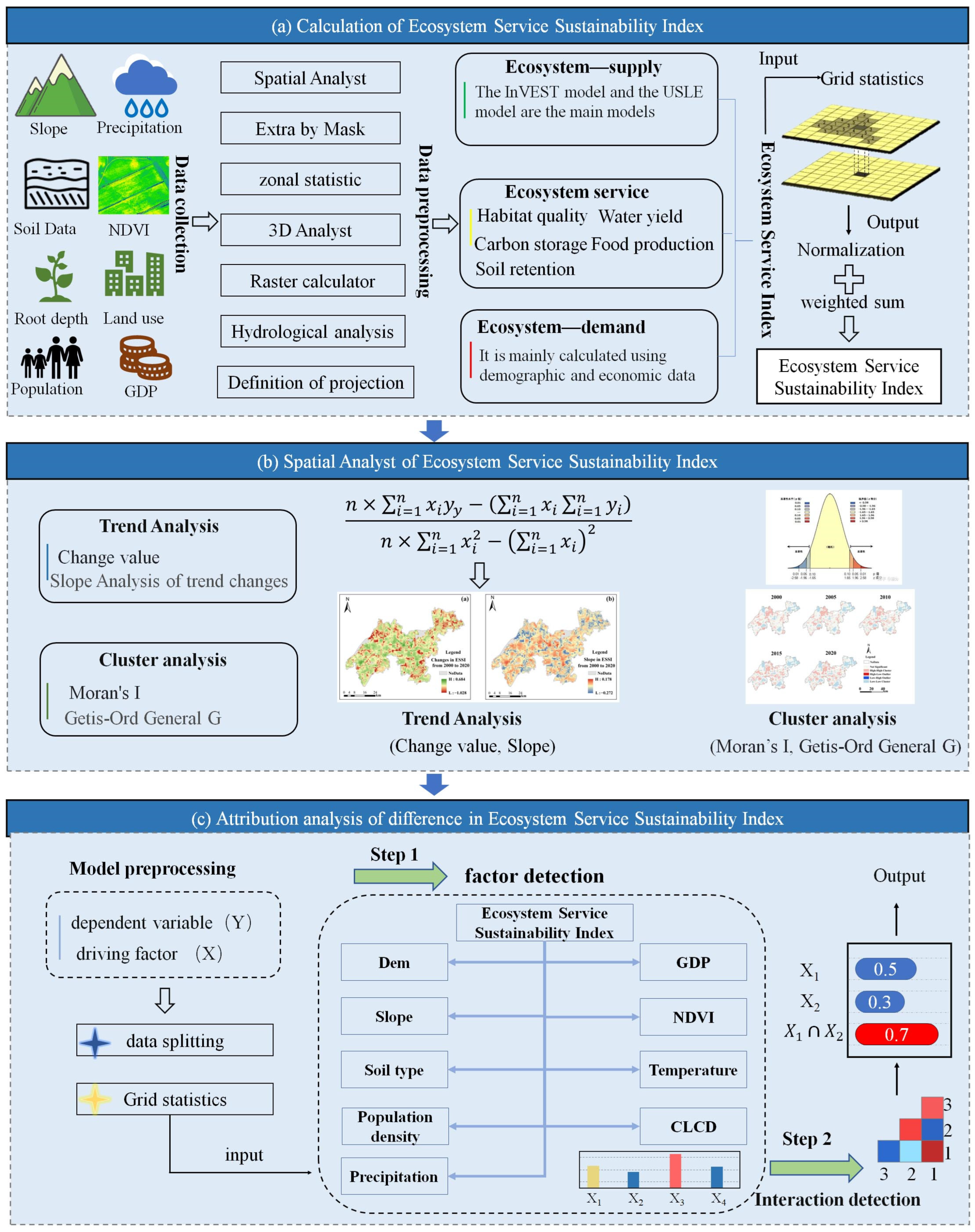
2.3. Methods
2.3.1. Evaluation of the Supply of Five ES Types

| ES Type | Formulas | Variables | |
|---|---|---|---|
| Supply Service | Habitat Quality [54] | : Habitat degradation degree of grid x in habitat type j. r: Threat source. y: Grid location of threat source r. : Weight of threat factor r (normalized across all threats). : Threat intensity value of threat source r in grid y. : Threat decay function from threat source r in grid y to grid x. : Accessibility/permeability level of threat sources to grid x. : Sensitivity of habitat type j to threat source r (0–1, where 1 = highly sensitive). : Habitat quality of grid x in habitat type j, derived from habitat suitability and degradation. : Habitat suitability index of habitat type j (0–1, where 1 = optimal suitability). h: Half-saturation parameter, controlling the nonlinear response of habitat quality to degradation. | |
| Water Yield [55] | : Annual water yield (mm) for land type j in grid x. : Annual actual evapotranspiration (mm) for land type j in grid x. : Annual precipitation (mm) in grid x. | ||
| Carbon Storage [56] | : Total carbon sequestration (t). : Aboveground biomass carbon stock (t). : Belowground soil carbon stock (t). : Belowground biomass carbon stock (t). : Carbon stock in dead organic matter (t). | ||
| Crop Production [56] | : Allocated food production for grid cell i. : Total food production. : Normalized difference vegetation index for grid cell i. : Sum of the normalized difference vegetation index across all cropland grid cells. | ||
| Soil Retention [56] | : Soil conservation amount for grid cell i. : Potential soil erosion amount for grid cell i. : Actual soil erosion amount for grid cell i. : Rainfall erosivity factor for grid cell i. : Soil erodibility factor for grid cell i. : Slope length factor for grid cell i. : Slope factor for grid cell i. : Water and soil retention factor for grid cell i. : Vegetation coverage factor for grid cell i. | ||
2.3.2. Evaluation of the Demand of Five ES Types
| ESs Type | Formulas | Variables | |
|---|---|---|---|
| Demand Services | Habitat Quality [54] | H: Demand for habitat quality. : Intensity of land use development, which is the percentage of construction land area relative to the total regional land area. : Population density, reflecting the human demand for habitat quality. : GDP per unit area. | |
| Water Yield [55] | : Total water demand (t). : Agricultural irrigation water demand (t). : Industrial water demand (t). : Domestic water demand (t). | ||
| Carbon Storage [61] | : Demand of carbon storage (t). : Per capita carbon emissions (t). : Population density (persons/km2). | ||
| Crop Production [61] | : Food demand. : Per capita food demand. : Population density within the grid. | ||
| Soil Retention [56] | : Actual soil erosion amount for grid cell i. : Rainfall erosivity factor for grid cell i. : Soil erodibility factor for grid cell i. : Slope length factor for grid cell i. : Slope factor for grid cell i. : Water and soil retention factor for grid cell i. : Vegetation coverage factor for grid cell i. | ||
2.3.3. Construction of ESSDI and ESSI
2.3.4. Calculation of the Spatial Autocorrelation Index and Change Trend Values
Calculation of the Spatial Autocorrelation Index
Calculation of the Change Trend Value
2.3.5. Principles of the Geodetector Model
3. Results
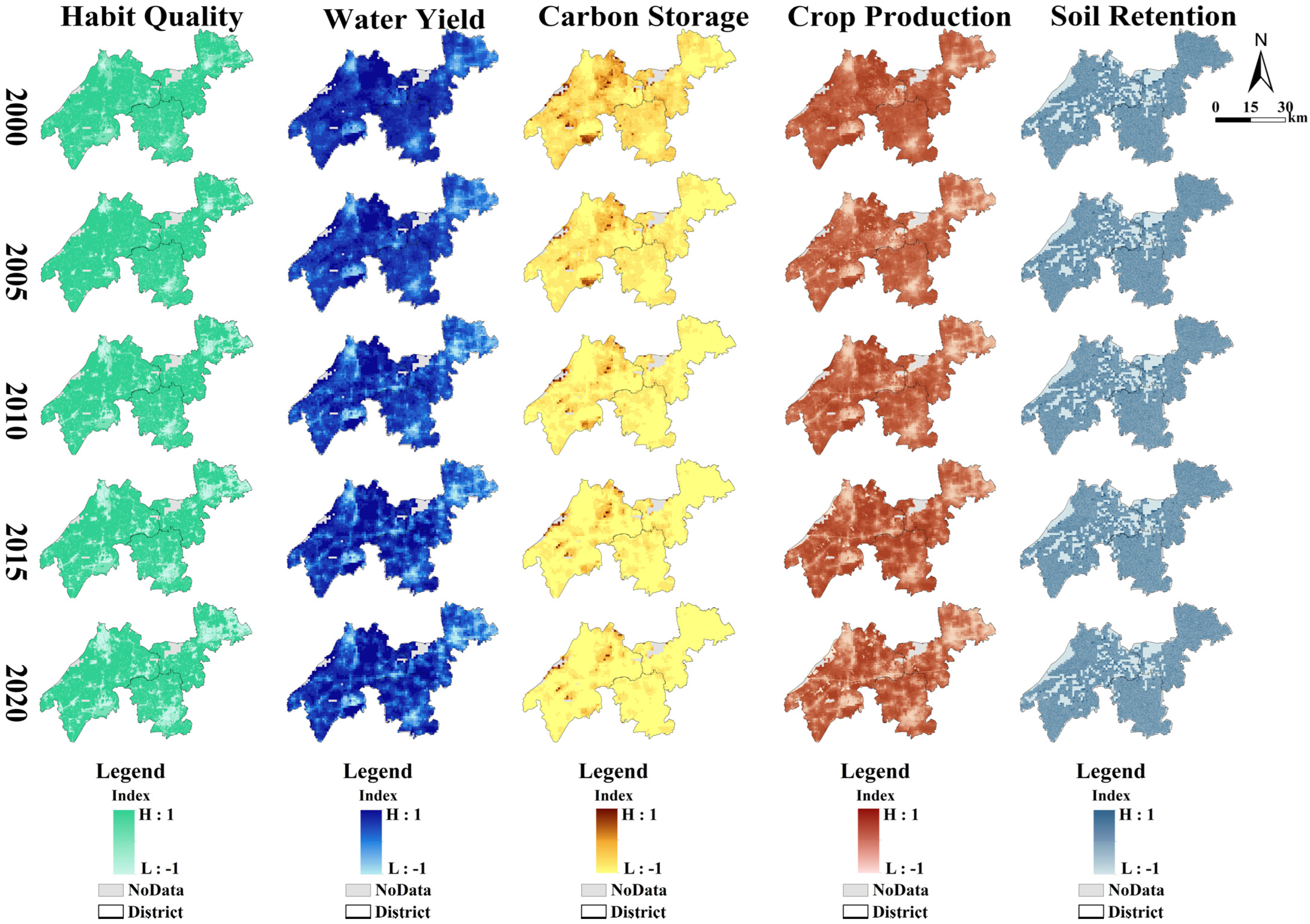
3.1. Spatiotemporal Change Analysis of ESSDI for the Five ES Types
3.2. Spatiotemporal Change Analysis of ESSI from 2000 to 2020 at Different Scales
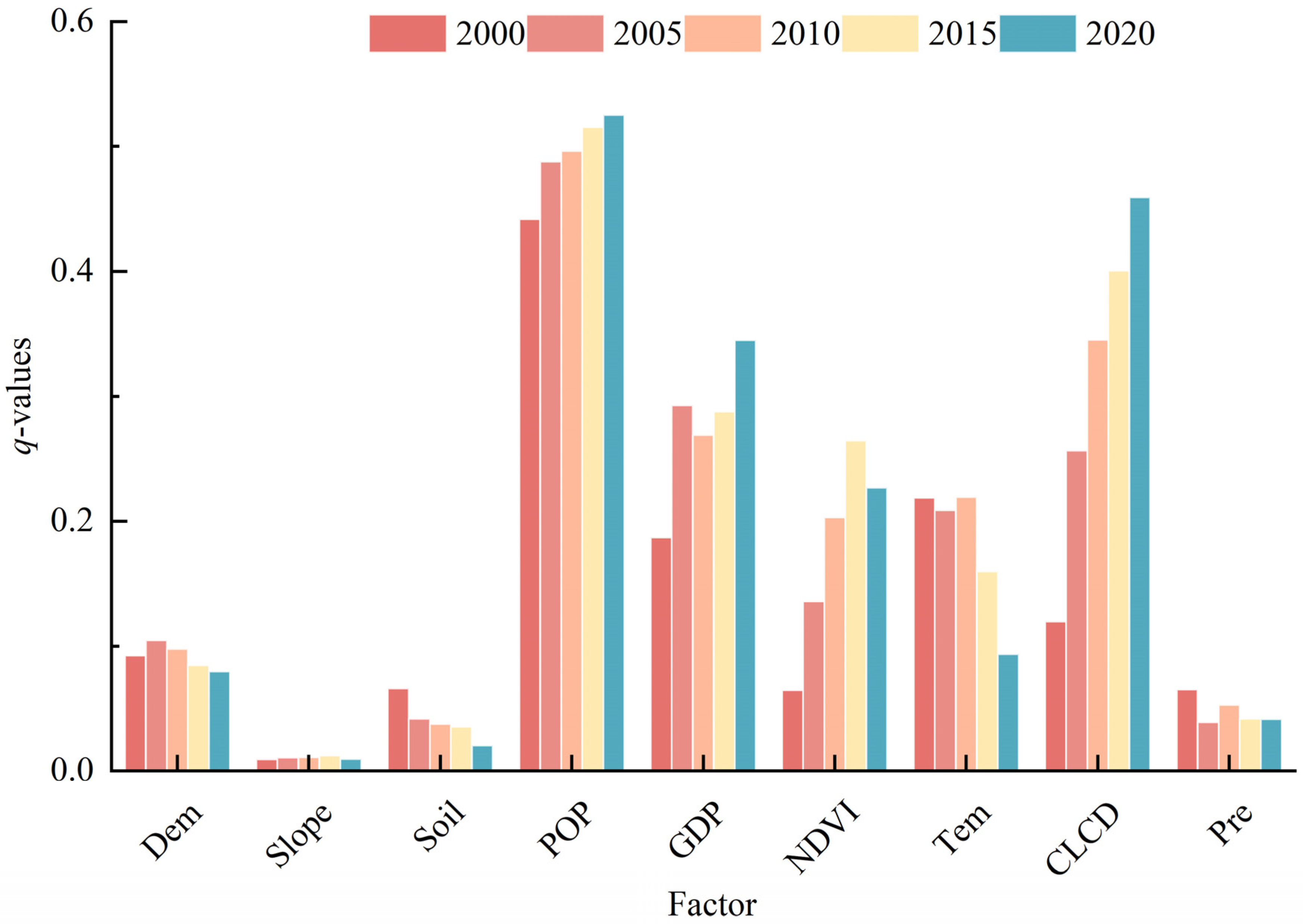
3.3. Driving Factor Analysis of ESSI
4. Discussion
4.1. Drivers of ESSDI and ESSI Changes in YRDIDZ
4.2. Theoretical Advancements, Limitations and Further Study
4.3. Implications for Global Deltaic Regions
5. Conclusions
Author Contributions
Funding
Institutional Review Board Statement
Informed Consent Statement
Data Availability Statement
Acknowledgments
Conflicts of Interest
Abbreviations
| CLCD | China Land Cover Dataset |
| DEM | Digital Elevation Model |
| ES | Ecosystem Service |
| ESSDI | Ecosystem Service Supply–Demand Index |
| ESSI | Ecosystem Service Sustainability Index |
| GDP | Gross Domestic Product |
| Gi* | Getis–Ord General G* |
| InVEST | Integrated Valuation of Ecosystem Services and Tradeoffs |
| LULC | Land Use and Land Cover |
| NDVI | Normalized Difference Vegetation Index |
| POP | Population Density |
| Pre | Precipitation |
| Tem | Temperature |
| YRDIDZ | Yangtze River Delta Integrated Demonstration Zone |
References
- Danley, B.; Widmark, C. Evaluating conceptual definitions of ecosystem services and their implications. Ecol. Econ. 2016, 126, 132–138. [Google Scholar] [CrossRef]
- He, J.; Zhou, Y.; Pandey, R.; Stringer, L.; Cao, Y.; Bhatt, H.; Luo, R.; Wang, S.; Li, T.; Li, S. Characteristics and Framework for Assessing Supply and Demand Relationship for Ecosystem Services Using a Trade-off and Synergy Lens. Land Degrad. Dev. 2025, 36, 1771–1786. [Google Scholar] [CrossRef]
- Fentaw, G.; Beneberu, G.; Wondie, A.; Eneyew, B. Ecosystem services of wetlands in the upper Abbay River basin, Ethiopia. Ecol. Indic. 2025, 171, 113142. [Google Scholar] [CrossRef]
- Ma, Y.; Yang, J. A review of methods for quantifying urban ecosystem services. Landsc. Urban Plan. 2025, 253, 105215. [Google Scholar] [CrossRef]
- Nolander, C.; Lundmark, R. A Review of Forest Ecosystem Services and Their Spatial Value Characteristics. Forests 2024, 15, 919. [Google Scholar] [CrossRef]
- Delgado, L.; Marín, V. Ecosystem services and ecosystem degradation: Environmentalist’s expectation? Ecosyst. Serv. 2020, 45, 101177. [Google Scholar] [CrossRef]
- Sutton, P.; Anderson, S.; Costanza, R.; Kubiszewski, I. The ecological economics of land degradation: Impacts on ecosystem service values. Ecol. Econ. 2016, 129, 182–192. [Google Scholar] [CrossRef]
- Sun, Y.; Zhang, X.; Ren, G.; Zwiers, F.; Hu, T. Contribution of urbanization to warming in China. Nat. Clim. Change 2016, 6, 706–709. [Google Scholar] [CrossRef]
- Lu, Y.; Zhang, Y.; Cao, X.; Wang, C.; Wang, Y.; Zhang, M.; Ferrier, R.; Jenkins, A.; Yuan, J.; Bailey, M.; et al. Forty years of reform and opening up: China’s progress toward a sustainable path. Sci. Adv. 2019, 5, eaau9413. [Google Scholar] [CrossRef]
- National Bureau of Statistics of the People’s Republic of China. China Statistical Yearbook (2024); China Statistics Press: Beijing, China, 2024.
- United Nations. World Urbanization Prospects: The 2013 Revision; United Nations: New York, NY, USA, 2014. [Google Scholar]
- Ji, Z.; Ren, H.; Zha, C.; Eshetu, S. Monitoring Spatio-Temporal Variations of Ponds in Typical Rural Area in the Huai River Basin of China. Remote Sens. 2024, 16, 39. [Google Scholar] [CrossRef]
- Mauri, A.; Girardello, M.; Forzieri, G.; Manca, F.; Beck, P.; Cescatti, A.; Strona, G. Assisted tree migration can reduce but not avert the decline of forest ecosystem services in Europe. Glob. Environ. Change 2023, 80, 102676. [Google Scholar] [CrossRef]
- Yan, F.; Zhang, S. Ecosystem service decline in response to wetland loss in the Sanjiang Plain, Northeast China. Ecol. Eng. 2019, 130, 117–121. [Google Scholar] [CrossRef]
- Tiemann, A.; Ring, I. Towards ecosystem service assessment: Developing biophysical indicators for forest ecosystem services. Ecol. Indic. 2022, 137, 108704. [Google Scholar] [CrossRef]
- Tedeschi, L.; Johnson, D.; Atzori, A.; Kaniyamattam, K.; Menendez, H., III. Applying Systems Thinking to Sustainable Beef Production Management: Modeling-Based Evidence for Enhancing Ecosystem Services. Systems 2024, 12, 446. [Google Scholar] [CrossRef]
- Cai, W.; Shu, C. Integrating System Perspectives to Optimize Ecosystem Service Provision in Urban Ecological Development. Systems 2024, 12, 375. [Google Scholar] [CrossRef]
- Yu, C.; Li, L.; Wei, H. Coupling Landscape Connectedness, Ecosystem Service Value, and Resident Welfare in Xining City, Western China. Systems 2023, 11, 512. [Google Scholar] [CrossRef]
- Zhou, L.; Guan, D.; Huang, X.; Yuan, X.; Zhang, M. Evaluation of the cultural ecosystem services of wetland park. Ecol. Indic. 2020, 114, 106286. [Google Scholar] [CrossRef]
- Wu, L.; Fan, F. Assessment of ecosystem services in new perspective: A comprehensive ecosystem service index (CESI) as a proxy to integrate multiple ecosystem services. Ecol. Indic. 2022, 138, 108800. [Google Scholar] [CrossRef]
- Ye, Y.; Bai, H.; Zhang, J.; Sun, D. A comparative analysis of ecosystem service values from various rice farming systems: A field experiment in China. Ecosyst. Serv. 2024, 70, 101664. [Google Scholar] [CrossRef]
- Liu, C.; Xu, H. Simulation and analysis of ecological early-warning of urban construction land expansion based on digital sensing feature recognition and remote sensing spatial analysis technology. Phys. Chem. Earth Parts A/B/C 2023, 132, 103484. [Google Scholar] [CrossRef]
- Eshetu, S.; Sha, J.; Li, X.; Bao, Z.; Ji, J.; Ji, Z.; Kassaye, A.; Lai, S.; Yang, Y. Ecosystem services dynamics and their influencing factors: Synergies/tradeoffs interactions and implications, the case of upper Blue Nile basin, Ethiopia. Sci. Total Environ. 2024, 938, 173524. [Google Scholar]
- Smith, G.; Day, B.; Binner, A. Multiple-Purchaser Payments for Ecosystem Services: An Exploration Using Spatial Simulation Modelling. Environ. Resour. Econ. 2019, 74, 421–447. [Google Scholar] [CrossRef]
- Perez-Verdin, G.; Sanjurjo-Rivera, E.; Galicia, L.; Hernandez-Diaz, J.; Hernandez-Trejo, V.; Marquez-Linares, M. Economic valuation of ecosystem services in Mexico: Current status and trends. Ecosyst. Serv. 2016, 21, 6–19. [Google Scholar] [CrossRef]
- Shahimoridi, R.; Kazemi, H.; Kamkar, B.; Nadimi, A.; Hosseinalizadeh, M.; Yeganeh, H. Economic valuation of ecosystem services in canola agroecosystems. Landsc. Ecol. Eng. 2024, 20, 427–438. [Google Scholar] [CrossRef]
- Sun, M.; Shen, X.; Xu, H.; Aili, A. Dynamics of ecosystem service values in the Tarim River Basin. Front. Environ. Sci. 2025, 12, 1484950. [Google Scholar] [CrossRef]
- Rey-Valette, H.; Mathé, S.; Salles, J. An assessment method of ecosystem services based on stakeholders perceptions: The Rapid Ecosystem Services Participatory Appraisal (RESPA). Ecosyst. Serv. 2017, 28, 311–319. [Google Scholar] [CrossRef]
- Ren, W.; Zhang, X.; Peng, H. The spatiotemporal changes and trade-off synergistic effects of ecosystem services in the Jianghan Plain of China under different scenarios. Environ. Res. Commun. 2024, 6, 035015. [Google Scholar] [CrossRef]
- Wang, Z.; Zhang, L.; Li, X.; Li, Y.; Fu, B. Integrating ecosystem service supply and demand into ecological risk assessment: A comprehensive framework and case study. Landsc. Ecol. 2021, 36, 2977–2995. [Google Scholar] [CrossRef]
- Lingua, F.; Coops, N.; Griess, V. Valuing cultural ecosystem services combining deep learning and benefit transfer approach. Ecosyst. Serv. 2022, 58, 101487. [Google Scholar] [CrossRef]
- Lu, Y.; Yang, J.; Peng, M.; Li, T.; Wen, D.; Huang, X. Monitoring ecosystem services in the Guangdong-Hong Kong-Macao Greater Bay Area based on multi-temporal deep learning. Sci. Total Environ. 2022, 822, 153662. [Google Scholar] [CrossRef]
- Kou, L.; Wang, X.; Wang, H.; Wang, X.; Hou, Y. Spatiotemporal analysis of ecological benefits coupling remote sensing ecological index and ecosystem services index. Ecol. Indic. 2024, 166, 112420. [Google Scholar] [CrossRef]
- Garshasbi, F.; Ashournejad, Q.; Ghalenoei, N. A comparative assessment of remote sensing based land cover products for economic valuation of ecosystem services of Hyrcanian forests. Adv. Space Res. 2025, 75, 4552–4574. [Google Scholar] [CrossRef]
- Wu, Q.; Yang, L.; Mi, J. Detecting the effects of opencast mining on ecosystem services value in arid and semi-arid areas based on time-series remote sensing images and Google Earth Engine (GEE). BMC Ecol. Evol. 2024, 24, 28. [Google Scholar] [CrossRef] [PubMed]
- Wang, H.; Wu, N.; Han, G.; Li, W.; Batunacun; Bao, Y. Analysis of spatial-temporal variations of grassland gross ecosystem product based on machine learning algorithm and multi-source remote sensing data: A case study of Xilinhot, China. Glob. Ecol. Conserv. 2024, 51, e02942. [Google Scholar] [CrossRef]
- Dingha, C.; Biber-Freudenberger, L.; Mbanga, L.; Kometa, S. Community-based valuation of wetland ecosystem services: Insights from Bamenda, Cameroon. Wetl. Ecol. Manag. 2025, 33, 14. [Google Scholar] [CrossRef]
- Mngadi, M.; Odindi, J.; Mutanga, O.; Sibanda, M. Quantitative remote sensing of forest ecosystem services in sub-Saharan Africa’s urban landscapes: A review. Environ. Monit. Assess. 2022, 194, 242. [Google Scholar] [CrossRef] [PubMed]
- Masenyama, A.; Mutanga, O.; Dube, T.; Bangira, T.; Sibanda, M.; Mabhaudhi, T. A systematic review on the use of remote sensing technologies in quantifying grasslands ecosystem services. GIScience Remote Sens. 2022, 59, 1000–1025. [Google Scholar] [CrossRef]
- Bi, J.; Lu, M.; Liu, F.; Cai, Y.; Wang, Y.; Duan, M.; Li, J.; Li, X.; Yu, D. Multi-scale urban ecosystem service changes and their impact mechanisms on human well-being. J. Environ. Manag. 2025, 374, 124117. [Google Scholar] [CrossRef]
- Zhang, C.; Su, B.; Beckmann, M.; Fang, S.; Xiao, Y.; Ma, H.; Yan, N.; Volk, M. Emergy-based valuation of glacier ecosystem services: A case from the Tibetan Plateau. J. Environ. Manag. 2025, 374, 123966. [Google Scholar] [CrossRef]
- Hirons, M.; Comberti, C.; Dunford, R. Valuing Cultural Ecosystem Services. Annu. Rev. Environ. Resour. 2016, 41, 545–574. [Google Scholar] [CrossRef]
- Comalada, F.; Llorente, O.; Acuña, V.; Saló, J.; Garcia, X. Using georeferenced text from social media to map the cultural ecosystem services of freshwater ecosystems. Ecosyst. Serv. 2025, 72, 101702. [Google Scholar] [CrossRef]
- Wang, H.; Huang, L.; Zhang, H.; Fu, Y.; Guo, W.; Jiao, X.; Zhou, H.; Zhu, Y. Development of a decision framework for river health and water yield ecosystem service in watershed. J. Hydrol. 2023, 623, 129773. [Google Scholar] [CrossRef]
- Yin, C.; Zhao, W.; Ye, J.; Muroki, M.; Pereira, P. Ecosystem carbon sequestration service supports the Sustainable Development Goals progress. J. Environ. Manag. 2023, 330, 117155. [Google Scholar] [CrossRef]
- Connor, J.; Summers, D.; Regan, C.; Abbott, H.; Linden, L.; Frizenschaf, J. Sensitivity analysis in economic evaluation of payments for water and carbon ecosystem services. Ecosyst. Serv. 2022, 54, 101416. [Google Scholar] [CrossRef]
- Thaweepworadej, P.; Evans, K. Tree-cover dynamics in a rapidly urbanising tropical mega-city—Are trees of greater biodiversity and ecosystem service value less likely to be lost? Urban For. Urban Green. 2025, 104, 128669. [Google Scholar] [CrossRef]
- Knegt, B.; Lof, M.; Clec’h, S.; Alkemade, R. Growing mismatches of supply and demand of ecosystem services in the Netherlands. J. Environ. Manag. 2025, 373, 123442. [Google Scholar] [CrossRef]
- Ren, E.; Lin, W.; Li, B.; Jiang, Y.; Zhang, Y.; Yu, Y. Regional Ecological Security Assessment Based on the Pressure–State–Response Framework: The Demonstration Zone of Yangtze River Delta as an Example. Land 2024, 13, 96. [Google Scholar] [CrossRef]
- Yan, F.; Wei, S.; Zhang, J.; Hu, B. Depth-to-bedrock map of China at a spatial resolution of 100 meters. Sci. Data 2020, 7, 2. [Google Scholar] [CrossRef] [PubMed]
- National Tibetan Plateau/Third Pole Environnent Data Center. China Soil Map Based Harmonized World Soil Database (HWSD) (v1.1) (2009); National Tibetan Plateau/Third Pole Environnent Data Center: Beijing, China, 2019. [Google Scholar]
- Liu, H.; Jiang, D.; Yang, X.; Luo, C. Spatialization Approach to 1km Grid GDP Supported by Remote Sensing. J. Geo-Inf. Sci. 2005, 7, 120–123. (In Chinese) [Google Scholar]
- Yang, J.; Dong, J.; Xiao, X.; Dai, J.; Wu, C.; Xia, J.; Zhao, G.; Zhao, M.; Li, Z.; Zhang, Y.; et al. Divergent shifts in peak photosynthesis timing of temperate and alpine grasslands in China. Remote Sens. Environ. 2019, 233, 111395. [Google Scholar] [CrossRef]
- Louis, V.; Page, S.; Tansey, K.; Jones, L.; Bika, K.; Balzter, H. Tiger Habitat Quality Modelling in Malaysia with Sentinel-2 and InVEST. Remote Sens. 2024, 16, 284. [Google Scholar] [CrossRef]
- Zhang, Z.; Zhang, Y.; Hu, Y.; Gao, J. Spatial and temporal distribution of supply-demand of ecosystem services in the demonstration zone of green and integrated ecological development of the Yangtze River Delta from the perspective of water-energy-food nexus. Acta Ecol. Sin. 2023, 43, 9430–9445. (In Chinese) [Google Scholar]
- Ding, S.; Jia, X.; Zhao, Y.; Qian, H.; Wang, H.; Kang, H.; Sun, Y. Spatial-temporal patterns of supply and demand of ecosystem services in the ecological function area of Qin-Ba Mountains. Ecol. Environ. Sci. 2023, 32, 2236–2248. (In Chinese) [Google Scholar]
- Gao, Z.; Wang, X.; Sun, X.; Wang, X.; Fan, Y.; Zhu, Q.; Lv, L. Multi-scenario prediction of habitat quality in Nanjing based on FLUS and InVEST models. J. Agric. Resour. Environ. 2022, 39, 1001–1013. (In Chinese) [Google Scholar]
- Gu, J.; Li, Y.; Du, W. Evaluation on water source conservation capacity and analysis of its variation characteristics of Taihu Lake Basin based on InVEST model. Water Resour. Prot. 2018, 34, 62–67. (In Chinese) [Google Scholar]
- Liu, Y.; Zhu, Y. Research of Carbon Storage Changes in Terrestrial Ecosystems Based on InVEST Model in the Yangtze River Delta Region. J. Nanjing Xiaozhuang Univ. 2020, 6, 82–90. (In Chinese) [Google Scholar]
- Li, P.; Tariq, A.; Li, Q.; Ghaffar, B.; Farhan, M.; Jamil, A.; Soufan, W.; Sabagh, A.; Freeshah, M. Soil erosion assessment by RUSLE model using remote sensing and GIS in an arid zone. Int. J. Digit. Earth 2023, 16, 3105–3124. [Google Scholar] [CrossRef]
- Peng, M.; Shao, Y.; Pei, B.; Yang, M.; Li, G.; Wen, W.; Yang, K. Spatial-temporal pattern and regional regulation of supply and demand of ecosystem services in the Yangtze River Delta integration demonstration zone. J. East China Norm. Univ. Nat. Sci. 2023, 6, 145–157. (In Chinese) [Google Scholar]
- Zhang, X.; Xiang, X.; Liu, H.; Wu, G. Practical Research on Carbon Dioxide Emission Calculation in Iron and Steel Industry. Ind. Saf. Environ. Prot. 2012, 38, 86–88. (In Chinese) [Google Scholar]
- Goodchild, M.F. Spatial Autocorrelation. In Catmog 47, Geo Books; University of East Anglia: Norwich, UK, 1986. [Google Scholar]
- Griffith, D. Spatial Autocorrelation: A Primer. Resource Publications in Geography; Association of American Geographers: Washington, DC, USA, 1987. [Google Scholar]
- Getis, A.; Ord, J.K. The analysis of spatial association by use of distance statistics. Geogr. Anal. 1992, 24, 189–206. [Google Scholar] [CrossRef]
- Ord, J.K.; Getis, A. Local Spatial Autocorrelation Statistics: Distributional Issues and an Application. Geogr. Anal. 1995, 27, 286–306. [Google Scholar] [CrossRef]
- Anselin, L. Local indicators of spatial association-LISA. Geogr. Anal. 1995, 27, 93–115. [Google Scholar] [CrossRef]
- Kulldorff, M. A spatial scan statistic. Commun. Stat. Theory Methods 1997, 26, 1481–1496. [Google Scholar] [CrossRef]
- Ji, J.; Tang, Z.; Zhang, W.; Liu, W.; Jin, B.; Xi, X.; Wang, F.; Zhang, R.; Guo, B.; Xu, Z.; et al. Spatiotemporal and Multiscale Analysis of the Coupling Coordination Degree between Economic Development Equality and Eco-Environmental Quality in China from 2001 to 2020. Remote Sens. 2022, 14, 737. [Google Scholar] [CrossRef]
- Zhao, H.; Chen, Y.; Zhou, Y.; Pei, T.; Xie, B.; Wang, X. Spatiotemporal variation of NDVI in vegetation growing season and its responses to climate factors in mid and eastern Gansu Province from 2008 to 2016. Arid. Land Geogr. 2019, 42, 1427–1435. (In Chinese) [Google Scholar]
- Wang, J.; Zhang, T.; Fu, B. A measure of spatial stratified heterogeneity. Ecol. Indic. 2016, 67, 250–256. [Google Scholar] [CrossRef]
- Li, Q.; Li, D.; Wang, J.; Wang, S.; Wang, R.; Fu, G.; Yuan, Y.; Zheng, Z. Spatial heterogeneity of ecosystem service bundles and the driving factors in the Beijing-Tianjin-Hebei region. J. Clean. Prod. 2024, 479, 144006. [Google Scholar] [CrossRef]
- Xue, Z.; Meng, X.; Liu, B. Spatiotemporal evolution and driving factors of ecosystem services in the upper Fenhe watershed, China. Ecol. Indic. 2024, 160, 111803. [Google Scholar] [CrossRef]
- Li, N.; Sun, P.; Zhang, J.; Mo, J.; Wang, K. Spatiotemporal evolution and driving factors of ecosystem services’ transformation in the Yellow River basin, China. Environ. Monit. Assess. 2024, 196, 252. [Google Scholar] [CrossRef]
- Wang, X.; Wu, J.; Liu, Y.; Hai, X.; Shanguan, Z.; Deng, L. Driving factors of ecosystem services and their spatiotemporal change assessment based on land use types in the Loess Plateau. J. Environ. Manag. 2022, 311, 114835. [Google Scholar] [CrossRef]
- Wang, H.; Yuan, W.; Ma, Y.; Bai, X.; Huang, L.; Cheng, S.; Yang, H.; Guo, W. Spatiotemporal dislocation of ecosystem supply and demand services from habitat quality under different development scenarios. Ecol. Indic. 2023, 157, 111230. [Google Scholar] [CrossRef]
- Yang, Y.; Li, M.; Feng, X.; Yan, H.; Su, M.; Wu, W. Spatiotemporal variation of essential ecosystem services and their trade-off/synergy along with rapid urbanization in the Lower Pearl River Basin, China. Ecol. Indic. 2021, 133, 108439. [Google Scholar] [CrossRef]
- Song, Y.; Wang, M.; Sun, X.; Fan, Z. Quantitative assessment of the habitat quality dynamics in Yellow River Basin, China. Environ. Monit. Assess. 2021, 193, 614. [Google Scholar] [CrossRef]
- Tao, Y.; Tao, Q.; Qiu, J.; Pueppke, S.; Gao, G.; Ou, W. Integrating water quantity- and quality-related ecosystem services into water scarcity assessment: A multi-scenario analysis in the Taihu Basin of China. Appl. Geogr. 2023, 160, 103101. [Google Scholar] [CrossRef]
- Zhao, Q.; Wang, Q. Water Ecosystem Service Quality Evaluation and Value Assessment of Taihu Lake in China. Water 2021, 13, 618. [Google Scholar] [CrossRef]
- Lun, F.; Xiao, Q.; Li, Q. The eutrophication variation analysis of Dianshan Lake from 2000 to 2020. Environ. Pollut. Control 2023, 45, 805–809+816. (In Chinese) [Google Scholar]
- Zhang, X.; Han, R.; Yang, S.; Yang, Y.; Tang, X.; Qu, W. Identification of bundles and driving factors of ecosystem services at multiple scales in the eastern China region. Ecol. Indic. 2024, 158, 111378. [Google Scholar] [CrossRef]
- Liu, W.; Zhan, J.; Zhao, F.; Wang, C.; Zhang, F.; Teng, Y.; Chu, X.; Kumi, M. Spatio-temporal variations of ecosystem services and their drivers in the Pearl River Delta, China. J. Clean. Prod. 2022, 337, 130466. [Google Scholar] [CrossRef]
- Liu, H.; Liu, S.; Wang, F.; Liu, Y.; Han, Z.; Wang, Q.; Yu, L.; Dong, Y.; Sun, J. Multilevel driving factors affecting ecosystem services and biodiversity dynamics on the Qinghai-Tibet Plateau. J. Clean. Prod. 2023, 396, 136448. [Google Scholar] [CrossRef]
- Shao, M.; Wu, L.; Li, F.; Lin, C. Spatiotemporal Dynamics of Ecosystem Services and the Driving Factors in Urban Agglomerations: Evidence from 12 National Urban Agglomerations in China. Front. Ecol. Evol. 2022, 10, 804969. [Google Scholar] [CrossRef]


| Name | Spatial and Temporal Resolution | Data Availability | Brief Description |
|---|---|---|---|
| LULC | 30 m 2000, 2005, 2010, 2015, 2020 | https://www.resdc.cn/DOI/DOI.aspx?DOIID=54 accessed on 10 September 2024 | A product of land use and land cover |
| Precipitation data | 30 m 2000, 2005, 2010, 2015, 2020 | https://data.cma.cn/ accessed on 1 April 2025 | A dataset for measuring regional precipitation amount |
| Depth-to-bedrock data | 100 m 2020 | https://doi.org/10.1038/s41597-019-0345-6 accessed on 13 September 2024 | A dataset for measuring the depth to bedrock |
| Soil data | 1000 m 2009 | https://data.tpdc.ac.cn/ accessed on 16 September 2024 | A dataset for measuring soil type, texture, etc. |
| DEM | 30 m 2009 | https://www.gscloud.cn/ accessed on 20 September 2024 | A dataset for measuring elevation |
| Population density | 100 m 2000, 2005, 2010, 2015, 2020 | https://www.worldpop.org accessed on 23 September 2024 | A dataset for measuring population spatial distribution |
| GDP data | 1000 m 2000, 2005, 2010, 2015, 2020 | https://www.resdc.cn/DOI/DOI.aspx?DOIID=33 accessed on 20 September 2024 | A dataset for measuring GDP spatial distribution |
| Evaporation data | 30 m 2000, 2005, 2010, 2015, 2020 | https://data.cma.cn/ accessed on 2 April 2025 | A dataset for measuring evaporation spatial distribution |
| NDVI data | 30 m 2000, 2005, 2010, 2015, 2020 | https://www.nesdc.org.cn accessed on 25 September 2024 | A dataset for measuring NDVI spatial distribution based on Landsat 5/7/8 images |
| Statistical yearbook | 2001, 2006, 2011, 2016, 2021 | Downloaded from governmental website accordingly | A dataset for recording socio-economic situation |
| Administrative division data | \ | http://www.ngcc.cn/ accessed on 5 September 2024 | A vector dataset for data clip and spatial analysis |
| LULC Type | HABITAT | CRP | URB |
|---|---|---|---|
| Grassland | 0.70 | 0.60 | 0.65 |
| Cropland | 0.50 | 0.25 | 0.50 |
| Wetland | 0.85 | 0.75 | 0.65 |
| Water | 0.80 | 0.65 | 0.75 |
| Forest | 0.90 | 0.70 | 0.80 |
| Built-up land | 0.00 | 0.00 | 0.00 |
| Name | LULC_veg | Root Depth (mm) | Kc |
|---|---|---|---|
| Grassland | 1.00 | 300.00 | 0.75 |
| Cropland | 1.00 | 3000.00 | 0.30 |
| Wetland | 1.00 | 500.00 | 0.60 |
| Water | 0.00 | 1.00 | 1.50 |
| Forest | 0.00 | 1.00 | 1.00 |
| Built-up land | 0.00 | 2.00 | 1.00 |
| LULC Type | Aboveground Carbon Density | Belowground Carbon Density | Soil Carbon Density | Dead Organic Carbon Density |
|---|---|---|---|---|
| Grassland | 17.37 | 20.85 | 105.85 | 2.94 |
| Cropland | 18.87 | 12.46 | 86.76 | 2.41 |
| Wetland | 0.00 | 0.00 | 81.10 | 0.00 |
| Water | 0.00 | 0.00 | 81.10 | 0.00 |
| Forest | 36.34 | 7.27 | 120.76 | 3.35 |
| Built-up land | 16.15 | 3.23 | 72.92 | 0.00 |
| ESs Type | District | Year | ||||
|---|---|---|---|---|---|---|
| 2000 | 2005 | 2010 | 2015 | 2020 | ||
| Habitat Quality | Qingpu | 0.68 | 0.70 | 0.58 | 0.50 | 0.42 |
| Jiashan | 0.70 | 0.70 | 0.65 | 0.58 | 0.52 | |
| Wujiang | 0.73 | 0.81 | 0.67 | 0.63 | 0.59 | |
| YRDIDZ | 0.68 | 0.70 | 0.58 | 0.50 | 0.42 | |
| Carbon Storage | Qingpu | −0.66 | −0.78 | −0.84 | −0.87 | −0.91 |
| Jiashan | −0.61 | −0.76 | −0.82 | −0.84 | −0.87 | |
| Wujiang | −0.50 | −0.65 | −0.72 | −0.76 | −0.80 | |
| YRDIDZ | −0.66 | −0.78 | −0.84 | −0.87 | −0.91 | |
| Water Yield | Qingpu | 0.39 | 0.24 | 0.25 | 0.26 | 0.27 |
| Jiashan | 0.54 | 0.44 | 0.43 | 0.49 | 0.49 | |
| Wujiang | 0.57 | 0.48 | 0.49 | 0.54 | 0.54 | |
| YRDIDZ | 0.39 | 0.24 | 0.25 | 0.26 | 0.27 | |
| Crop Production | Qingpu | 0.28 | 0.07 | 0.10 | 0.19 | 0.02 |
| Jiashan | 0.45 | 0.30 | 0.32 | 0.43 | 0.27 | |
| Wujiang | 0.41 | 0.25 | 0.31 | 0.35 | 0.21 | |
| YRDIDZ | 0.28 | 0.07 | 0.10 | 0.19 | 0.02 | |
| Soil Retention | Qingpu | 0.54 | 0.54 | 0.54 | 0.54 | 0.53 |
| Jiashan | 0.56 | 0.56 | 0.56 | 0.56 | 0.56 | |
| Wujiang | 0.48 | 0.48 | 0.48 | 0.48 | 0.48 | |
| YRDIDZ | 0.54 | 0.54 | 0.54 | 0.54 | 0.53 | |
| Scale | Year | ||||
|---|---|---|---|---|---|
| 2000 | 2005 | 2010 | 2015 | 2020 | |
| Qingpu | 0.33 | 0.25 | 0.23 | 0.24 | 0.19 |
| Jiashan | 0.25 | 0.16 | 0.13 | 0.13 | 0.07 |
| Wujiang | 0.34 | 0.28 | 0.25 | 0.25 | 0.21 |
| YRDIDZ | 0.31 | 0.24 | 0.21 | 0.22 | 0.17 |
| District Name | Town Name | Year | ||||
|---|---|---|---|---|---|---|
| 2000 | 2005 | 2010 | 2015 | 2020 | ||
| Qingpu | Baihe | 0.34 | 0.24 | 0.19 | 0.18 | 0.14 |
| Huaxin | 0.01 | −0.08 | −0.15 | −0.18 | −0.24 | |
| Jinze | 0.40 | 0.30 | 0.30 | 0.32 | 0.26 | |
| Liantang | 0.40 | 0.32 | 0.30 | 0.30 | 0.25 | |
| Xiayang | 0.00 | −0.07 | −0.12 | −0.11 | −0.15 | |
| Xianghuaqiao | 0.13 | 0.07 | 0.02 | 0.01 | −0.07 | |
| Xujing | −0.04 | −0.14 | −0.19 | −0.22 | −0.28 | |
| Yingpu | −0.08 | −0.16 | −0.17 | −0.18 | −0.24 | |
| Zhaoxiang | 0.16 | 0.04 | 0.02 | 0.01 | −0.07 | |
| Zhonggu | 0.32 | 0.22 | 0.18 | 0.17 | 0.11 | |
| Zhujiajiao | 0.34 | 0.23 | 0.22 | 0.24 | 0.19 | |
| Jiashan | Dayun | 0.37 | 0.30 | 0.27 | 0.29 | 0.25 |
| Ganyao | 0.33 | 0.25 | 0.24 | 0.26 | 0.21 | |
| Huimin | 0.29 | 0.21 | 0.18 | 0.18 | 0.11 | |
| Luoxing | 0.17 | 0.09 | 0.01 | 0.02 | −0.05 | |
| Taozhuang | 0.40 | 0.32 | 0.31 | 0.34 | 0.28 | |
| Tianning | 0.43 | 0.34 | 0.33 | 0.34 | 0.30 | |
| Weitang | 0.08 | 0.02 | 0.01 | 0.02 | −0.03 | |
| Xitang | 0.38 | 0.33 | 0.33 | 0.36 | 0.30 | |
| Yaozhuang | 0.40 | 0.30 | 0.25 | 0.26 | 0.21 | |
| Wujiang | Tongli | 0.38 | 0.31 | 0.27 | 0.25 | 0.21 |
| Lili | 0.33 | 0.25 | 0.25 | 0.27 | 0.23 | |
| Shengze | 0.24 | 0.22 | 0.16 | 0.14 | 0.10 | |
| Taihuxincheng | 0.35 | 0.27 | 0.23 | 0.23 | 0.17 | |
| Qidu | 0.36 | 0.29 | 0.27 | 0.26 | 0.21 | |
| Taoyuan | 0.35 | 0.30 | 0.29 | 0.30 | 0.26 | |
| Zhenze | 0.31 | 0.25 | 0.23 | 0.25 | 0.20 | |
| Pingwang | 0.39 | 0.35 | 0.32 | 0.32 | 0.29 | |
Disclaimer/Publisher’s Note: The statements, opinions and data contained in all publications are solely those of the individual author(s) and contributor(s) and not of MDPI and/or the editor(s). MDPI and/or the editor(s) disclaim responsibility for any injury to people or property resulting from any ideas, methods, instructions or products referred to in the content. |
© 2025 by the authors. Licensee MDPI, Basel, Switzerland. This article is an open access article distributed under the terms and conditions of the Creative Commons Attribution (CC BY) license (https://creativecommons.org/licenses/by/4.0/).
Share and Cite
Zhu, Z.; Xu, C.; Ji, J.; Wang, L.; Zhang, W.; Wang, L.; Shifaw, E.; Zhang, W. Spatiotemporal Changes and Driving Forces of the Ecosystem Service Sustainability in Typical Watertown Region of China from 2000 to 2020. Systems 2025, 13, 340. https://doi.org/10.3390/systems13050340
Zhu Z, Xu C, Ji J, Wang L, Zhang W, Wang L, Shifaw E, Zhang W. Spatiotemporal Changes and Driving Forces of the Ecosystem Service Sustainability in Typical Watertown Region of China from 2000 to 2020. Systems. 2025; 13(5):340. https://doi.org/10.3390/systems13050340
Chicago/Turabian StyleZhu, Zhenhong, Chen Xu, Jianwan Ji, Liang Wang, Wanglong Zhang, Litao Wang, Eshetu Shifaw, and Weiwei Zhang. 2025. "Spatiotemporal Changes and Driving Forces of the Ecosystem Service Sustainability in Typical Watertown Region of China from 2000 to 2020" Systems 13, no. 5: 340. https://doi.org/10.3390/systems13050340
APA StyleZhu, Z., Xu, C., Ji, J., Wang, L., Zhang, W., Wang, L., Shifaw, E., & Zhang, W. (2025). Spatiotemporal Changes and Driving Forces of the Ecosystem Service Sustainability in Typical Watertown Region of China from 2000 to 2020. Systems, 13(5), 340. https://doi.org/10.3390/systems13050340