Continuous Fiber Angle Topology Optimization for Polymer Composite Deposition Additive Manufacturing Applications

Abstract

Mechanical properties of parts produced with polymer deposition additive manufacturing (AM) depend on the print bead direction, particularly when short carbon-fiber reinforcement is added to the polymer feedstock. This offers a unique opportunity in the design of these structures since the AM print path can potentially be defined in a direction that takes advantage of the enhanced stiffness gained in the bead and, therefore, fiber direction. This paper presents a topology optimization approach for continuous fiber angle optimization (CFAO), which computes the best layout and orientation of fiber reinforcement for AM structures. Statically loaded structures are designed for minimum compliance where the adjoint variable method is used to compute design derivatives, and a sensitivity filter is employed to reduce the checkerboard effect. The nature of the layer-by-layer approach in AM is given special consideration in the algorithm presented. Examples are provided to demonstrate the applicability of the method in both two and three dimensions. The solution to our two dimensional problem is then printed with a fused filament fabrication (FFF) desktop printer using the material distribution results and a simple infill method which approximates the optimal fiber angle results using a contour-parallel deposition strategy. Mechanical stiffness testing of the printed parts shows improved results as compared to structures designed without accounting for the direction of the composite structure. Results show that the mechanical properties of the final FFF carbon fiber/polymer composite printed parts are greatly influenced by the print direction, and optimized material orientation tends to align with the imposed force direction to minimize the compliance.

1. Introduction

Carbon-fiber-filled polymer composites continue to provide unique engineering solutions for lightweight structures in industries such as automotive and aerospace. It is well understood that the mechanical properties of thermoplastic polymers can be greatly improved by adding short carbon or glass fibers to the polymer matrix, making it possible to produce structures having superior performance with existing tooling. This is true in today’s additive manufacturing (AM) where small-scale three-dimensional (3D) printer filament suppliers now offer carbon-fiber-filled products for the fused filament fabrication (FFF) process (also known as fused filament deposition (FDM)). The success of polymer composite large-scale additive manufacturing (LSAM) is due in part to the improved mechanical performance gained when short carbon-fiber polymers are employed. A unique design opportunity emerged for fiber-reinforced polymer composite AM since the direction of the non-isotropic print bead can potentially be designed to give the best overall structural performance. The design freedom afforded by AM requires new design approaches such as that provided by topology optimization, which determines the best layout of a structure without the limitations typically imposed by traditional manufacturing methods.

Fused filament fabrication (FFF) uses polymer-based feedstock as input to make parts from digital design data where a material orientation is defined by the print direction. In FFF, polymer or polymer composite filament is forced through a heated nozzle where the molten material is deposited onto a platform to print a part in a layer-by-layer fashion. The non-isotropic mechanical properties of the printed parts depend greatly on the deposited material and the orientation of the printed bead [1,2,3], especially when the feedstock polymer is blended with short carbon fibers. In addition, topology optimization (see, e.g., Bendsøe and Sigmund [4]) enjoys a long history in mechanical part design, and it has also become very popular in the design of AM structures [5,6,7,8,9,10]. With the presence of short carbon fibers, the computation of optimal structures must incorporate the non-isotropic response of the material, making it necessary to solve for optimal material distribution in addition to the optimal material angle orientation distribution. This paper focuses on the use of short fiber/polymer composites in the FFF process; however, the design method presented here is equally applicable to other AM processes that result in oriented microstructures.

1.1. Polymer Composite Deposition Additive Manufacturing

Polymer deposition AM can be categorized into two main areas. The first one is for small-scale 3D printing application, which uses continuous filament as the feedstock commonly known as FFF. FFF has a continually growing market [11] and is popular among hobbyists, in academic research, for rapid prototyping, and for select industrial final products. There are several drawbacks in small-scale FFF. The size of the objects is relatively small, mostly smaller than one cubic foot. The dominant type of the feedstock for small-scale FFF is thermoplastic, which has weaker mechanical properties than metals, limiting its use for final part production in industry. Various polymer composite filaments were introduced to improve the filament’s mechanical properties [12,13,14,15,16,17,18,19,20]. One approach for improving mechanical performance is to blend short carbon fiber (CF) within the thermoplastic feedstock to form a CF/polymer filament. Researchers showed that parts made of CF/polymer filament have improved tensile strength and stiffness as compared to those made from unfilled polymer filament [18,19,20]. Adding CF to the polymer feedstock also reduces print-induced warpage of the structure [21], due in part to the relative lower coefficient of thermal expansion and higher thermal conductivity of the CF.

The second category of polymer deposition AM is large-scale 3D printing. This process aims to print objects in large size, with polymer nozzle exit diameters exceeding 6.35 mm. Large-scale 3D printing is a more recent innovation, and the most prominent example is large-scale additive manufacturing (LSAM) technology [22]. LSAM systems print with a single screw extruder attached to a large gantry system and discontinuous CF polymer pellets. LSAM requires lower energy input and gives higher material output per unit time than small-scale 3D printing [23]. Examples include the big area additive manufacturing (BAAM) system [22] in addition to others who created custom large-scale 3D printers and print objects with CF/polymer pellets (cf. Reference [24]). The adoption of large-scale 3D printing is pushing the application of polymer/short fiber composite deposition to new industrial applications.

Research on FFF with CF/polymer feedstock shows that the fibers become highly aligned along the printing direction [18,20,25], forming a non-isotropic microstructure having mechanical strength and stiffness that is much higher along the bead axis than across the bead. Furthermore, it is possible to predict the mechanical property of the short fiber composite printed part which is needed for part design [25,26].

1.2. Topology Optimization and Additive Manufacturing

Topology optimization is a finite-element-based computational tool commonly used to compute the optimum layout of a structure within a prescribed design domain [4]. Optimal structures are obtained by minimizing a certain objective value, given prescribed design constraints. In structural mechanics, it is common to minimize the compliance of a structure, thus maximizing its stiffness, while constraining the amount of material used in the design. There are numerous topology optimization approaches, including homogenization method [27,28], solid isotropic material method (SIMP) [29,30,31,32,33,34], evolutionary structural optimization method (ESO) [35], and bidirectional structural optimization method (BESO) [36].

Topology optimization enjoys widespread application, particularly in additive manufacturing. Sundararajan [5] applied the homogenization method with a smoothing scheme to optimize the Messerschimitt–Bölkow–Blohm (MBB) and a cantilever beam. The optimized shape was assembled using mesostructures through elements with a square void. Zhang et al. [10] employed the homogenization, optimization, and construction (HOC) technique to design variable cellular structures. In Zhang’s paper, the cellular structure was constructed based on the optimized density distribution using the SIMP method, and the part was fabricated with stereolithography. Gaynor et al. [6] implemented the original, combinatory, and multiphase SIMP approaches to optimize the shape of compliant mechanisms. Their research showed that an optimized topology can be obtained using more than one material, and then it can be built using the multimaterial Polyjet 3D printing technique. Wang et al. [7] also presented a review on AM of porous metals for orthopedic implants. Furthermore, numerical methods were proposed to overcome the overhang limitation of the 3D printed parts [8,9].

1.3. Simultaneous Topology and Fiber Orientation Optimization

Development and application of topology optimization includes both isotropic material and non-isotropic material response (see, e.g., Bendsøe and Sigmund [4]). The penalized material density approach that provides a basis for our work appears as the density method in Yang and Chuang [37], and more recently as the SIMP method (cf. Bendsøe and Sigmund [4]) which saw extensive development and application in structural design problems. Early topology optimizations based on the homogenization method (cf. Bendsøe and Kikuchi [27]) considered composite structures with continuously varying material orientation and distribution. While the homogenization approach saw extensive developments over the past three decades [27], application of the method is limited to non-discrete (0-1) layout structures, thus making it of limited use in additive manufacturing.

In this paper, we are particularly interested in extending the SIMP method for AM structures having oriented microstructures such as polymer composite FFF. The SIMP method (see, e.g., Reference [4]) employs an isotropic material model in each discretized finite element where a penalization parameter is imposed to drive the solution field to a discrete (0-1) layout. The original SIMP method was modified to accommodate anisotropic materials, referred to as solid orthotropic material penalization (SOMP) in [38], but is yet to be applied to polymer composite AM. Extensions of the SIMP method were proposed [39,40] to accommodate in-plane angle design variability, which is ideally suited for these applications. Previously, Jia et al. [38] applied the SIMP method with material orientation design variables to a fiber-reinforced composite for minimum compliance. The optimized topology appears with minor checkerboard effect, as no anti-checkerboarding filter [41,42] was employed. Setoodeh et al. [43] developed a stress-based approach combined with cellular automata using the SIMP method to solve for minimum compliance. They further extended their approach to problems with multiple loads, though the fiber angle update scheme was based on a random search. Nomura et al. [44] proposed a general topology optimization method that simultaneously optimized both material distribution and material orientation based on discrete angle sets. Their orientation variables are defined by Cartesian components and include a relaxation of the orientation design space. Our previous topology optimization work appeared in Hoglund and Smith [45,46,47] which considered fixed fiber directions and extended the SIMP method to accommodate orientation design variables where design sensitivities with respect to both the density and material orientation were derived and implemented in a finite-element-based design program. In this approach, the density sensitivity was filtered using a linear weighted-average filter [41,42], thus avoiding common topology optimization checkerboarding issues.

Many of the aforementioned optimization schemes for material distribution and material orientation are limited to two-dimensional problems without considering the three-dimensional (3D) aspects of the AM design space. Indeed, the literature has yet to address topology material distribution and orientation optimization for 3D AM applications such as polymer composite FFF. Therefore, this paper proposes a design optimization approach that optimizes material distribution and material orientation for AM structures with oriented microstructures. Examples include structures having 2D layouts, and another having a 3D layout. Testing included in this paper illustrates the effectiveness of the 2D optimized structures. An important assumption in 3D design is that, since the AM parts are made through a layer-by-layer process, material orientation is constrained to the print plane. This assumption is applicable to polymer composite FFF since fibers are highly aligned along the print direction. The design approach given here will provide insight into the optimal topology and the bead pattern of the printed part, thus making the AM designs more efficient and competitive in the market.

2. Methodology

2.1. CFAO Topology Optimization Formulation

The common topology optimization problem is to minimize the compliance of a structure subject to constraints on material usage and equilibrium. The traditional topology optimization problem (see, e.g., Bendsøe and Sigmund [4]) is extended here to include both material density and fiber orientation for AM, which may be written mathematically as shown below.

$$\mathrm{Minimize}:c\left(\mathsf{\rho },\mathsf{\theta }\right)=U{\left(\mathsf{\rho },\mathsf{\theta }\right)}^{T}F,$$

(1)

$$\mathrm{Subject}\mathrm{to}:\{\begin{array}{c}\frac{v\left(\mathsf{\rho }\right)}{V_0}=f\\ K\left(\mathsf{\rho },\mathsf{\theta }\right)U\left(\mathsf{\rho },\mathsf{\theta }\right)=F\\ {\rho }_{min}\le {\rho }_{\mathrm{e}}\le 1\\ -2\mathsf{\pi }\le {\theta }_{\mathrm{e}}\le 2\mathsf{\pi }\end{array},$$

(2)

where the compliance c is the objective function in the optimization, written here as a function of the density and material angle design variable vectors $\mathsf{\rho }$ and $\mathsf{\theta }$, respectively. The vectors $\mathsf{\rho }=\left[{\rho }_1{\rho }_2\cdots {\rho }_N\right]$ and $\mathsf{\theta }=\left[{\theta }_1{\theta }_2\cdots {\theta }_N\right]$ are defined, respectively, by element density design variables ${\rho }_e,e=1,\cdots ,N$ and element material angle design variables ${\theta }_e,e=1,\cdots ,N$, where N is the number of elements in the finite element model. Since AM processes such as FFF deposit material in a layer-by-layer fashion, element material angle is assumed to only vary within the print plane. Therefore, each element e contains only two design variables: one element density ${\rho }_e$ and one material angle ${\theta }_e$.

The compliance objective function c in Equation (1) is written in terms of the finite element global stiffness matrix K, displacement vector U, and load vector F in the usual manner (cf. Sigmund [32]). The first constraint in Equation (2) is imposed on the design volume $v\left(\mathsf{\rho }\right)$ limiting it to a prescribed volume fraction f ($0\le f\le 1$) of the total design domain volume $V_0$. The second constraint imposes equilibrium on the design where it is noted that the stiffness matrix $K=K\left(\mathsf{\rho },\mathsf{\theta }\right)$ and the displacement vector $U=U\left(\mathsf{\rho },\mathsf{\theta }\right)$ are design-dependent. We assume here that the applied loads in F are not a function of the design variables.

Also included in Equation (2) are simple bounds on element density and element material angle. The former imposes a lower bound of ${\rho }_{min}$ on element density to avoid singularity issues in the finite element stiffness matrix K. The upper bond on each ${\rho }_e$ of unity allows for an element to realize full material utilization. Simple bounds on each ${\theta }_e$ of ±2π allow for angle rotation into the optimal orientation without restriction. This simple approach was shown to work well in the examples considered here while avoiding the added computation required in other shape-function-based approaches used to define orientation angle (see, e.g., Nomura et al. [44] and Xia and Shi [48]).

The stiffness matrix $K=K\left(\mathsf{\rho },\mathsf{\theta }\right)$ is assembled through contributions from each element stiffness matrix k_e(${\rho }_e,{\theta }_e$) (given below) as

$$K\left(\mathsf{\rho },\mathsf{\theta }\right)={\displaystyle \sum }_{\mathrm{e}=1}^{\mathrm{N}}{\left({\rho }_{\mathrm{e}}\right)}^p{k}_e\left({\theta }_{\mathrm{e}}\right),$$

(3)

where a penalization parameter $p$ is imposed on each element density variable, which tends to drive the element density ${\rho }_{\mathrm{e}}$ to its lower or upper limit. Equation (3) extends the SIMP method proposed by Sigmund [32] by including an anisotropic element stiffness matrix $k_e\left({\theta }_{\mathrm{e}}\right)$ which is written here in terms of the element material angle variable ${\theta }_{\mathrm{e}}$ as proposed by Hoglund and Smith [46] and also Jia et al. [38]. It follows that the compliance objective function c in Equation (1) may be written in terms of the element stiffness matrices $k_e$ and element displacement vectors $u_e$ as

$$c\left(\mathsf{\rho },\mathsf{\theta }\right)={\displaystyle \sum }_{\mathrm{e}=1}^{\mathrm{N}}{\left({\rho }_{\mathrm{e}}\right)}^{\mathrm{p}}{u}_e^{\mathrm{T}}{k}_e\left({\theta }_{\mathrm{e}}\right)u_e,$$

(4)

which simplifies the evaluation of the compliance in the optimization calculations by making it an element-by-element computation.

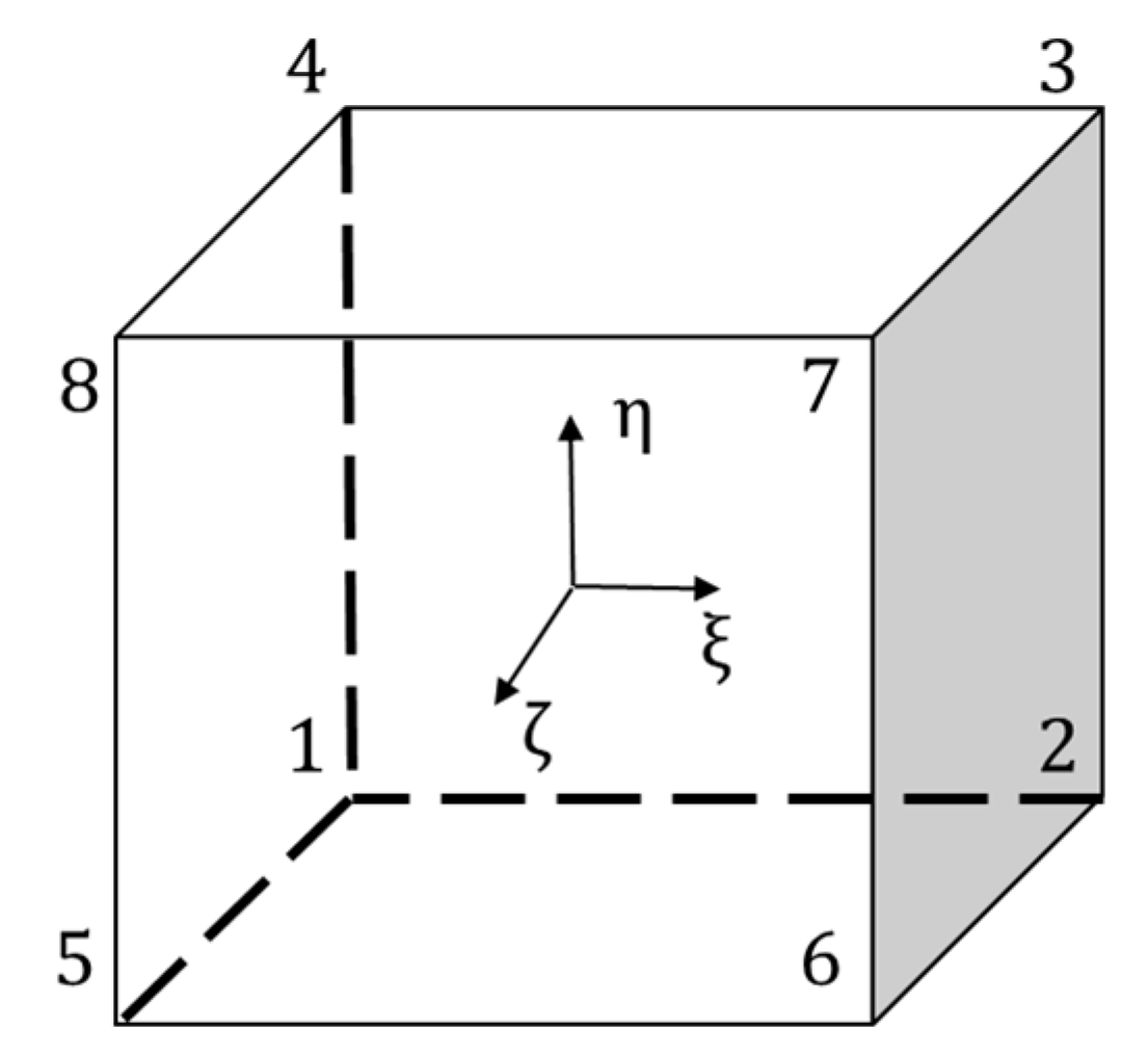
2.2. Isoparametric Hexagonal Element

In our analyses, the elemental stiffness matrix $k_e$ is defined using the eight-node isoparametric hexahedral element [49] shown in Figure 1.

The element stiffness matrix is obtained in the usual manner (see, e.g., the finite element text by Huebner et al. [49]) where element integrations are performed with Gauss quadrature as

$$\begin{array}{ll}{k}_e\left({\theta }_e\right)& ={{\displaystyle \iiint }}_{{\mathsf{\Omega }}_{\mathrm{e}}}{B}^{\mathrm{T}}{C}^{\prime }\left({\theta }_e\right)B\mathrm{d}\mathsf{\Omega }\\ & \approx {\displaystyle {\displaystyle \sum }_{\mathrm{i}=1}^{n_{gp}}}{\displaystyle {\displaystyle \sum }_{\mathrm{j}=1}^{n_{gp}}}{\displaystyle {\displaystyle \sum }_{\mathrm{k}=1}^{n_{gp}}}\left(W_i{W}_j{W}_{k}B{\left({\xi }_i,{\eta }_j,{\zeta }_k\right)}^{\mathrm{T}}{C}^{\prime }\left({\theta }_e\right)B\left({\xi }_i,{\eta }_j,{\zeta }_k\right)\left|J\left({\xi }_i,{\eta }_j,{\zeta }_k\right)\right|\right),\end{array}$$

(5)

where $n_{gp}$ is the number of Gauss points for the integrals in each of the three coordinate directions, and $B$ is the strain–displacement matrix defined by derivatives of the element shape functions in the usual manner. The element angle ${\theta }_{\mathrm{e}}$ is used to define the rotated constitutive matrix $C^{\prime }\left({\theta }_{\mathrm{e}}\right)$ in Equation (5) in terms of the original constitutive matrix $C$ as [50]

$$C^{\prime }\left({\theta }_e\right)=T{\left({\theta }_e\right)}^{-1}CT{\left({\theta }_e\right)}^{-\mathrm{T}}.$$

(6)

We assume that the plane formed by axes $\xi$ and $\eta$ in Figure 1 is the AM print plane, such that a rotation about the $\zeta$ axis by an angle $\theta$ with respect to the positive $\xi$ direction defines the material direction within the element. The resulting rotation matrix $T\left(\theta \right)$ for each element is evaluated through T⁻¹ as

$$T^{-1}\left(\theta \right)=\left[\begin{array}{cccccc}\cos {\left(\theta \right)}^2& \sin {\left(\theta \right)}^2& 0& 0& 0& -2\cos \left(\theta \right)\sin \left(\theta \right)\\ \sin {\left(\theta \right)}^2& \cos {\left(\theta \right)}^2& 0& 0& 0& 2\cos \left(\theta \right)\sin \left(\theta \right)\\ 0& 0& 1& 0& 0& 0\\ 0& 0& 0& \cos \left(\theta \right)& \sin \left(\theta \right)& 0\\ 0& 0& 0& -\sin \left(\theta \right)& \cos \left(\theta \right)& 0\\ \cos \left(\theta \right)\sin \left(\theta \right)& -\cos \left(\theta \right)\sin \left(\theta \right)& 0& 0& 0& \cos {\left(\theta \right)}^2-\sin {\left(\theta \right)}^2\end{array}\right].$$

(7)

We consider AM materials that may be modeled using transversely isotropic material symmetry [51]. Considering xyz-space, the transversely isotropic constitutive tensor $C$ having a primary axis in the x-direction may be written in terms of the elastic moduli E_x and E_y, the Poison’s ratios ${\nu }_{xy}$ and ${\nu }_{yx}$, and shear modulus G_xy, as follows [51]:

$$C={\left[\begin{array}{cccccc}\frac{1}{E_x}& -\frac{{\nu }_{xy}}{E_x}& -\frac{{\nu }_{xy}}{E_x}& 0& 0& 0\\ -\frac{{\nu }_{xy}}{E_x}& \frac{1}{E_y}& -\frac{{\nu }_{yz}}{E_y}& 0& 0& 0\\ -\frac{{\nu }_{xy}}{E_x}& -\frac{{\nu }_{yz}}{E_y}& \frac{1}{E_y}& 0& 0& 0\\ 0& 0& 0& \frac{2\left(1+{\nu }_{yz}\right)}{E_y}& 0& 0\\ 0& 0& 0& 0& \frac{1}{G_{xy}}& 0\\ 0& 0& 0& 0& 0& \frac{1}{G_{xy}}\end{array}\right]}^{-1}.$$

(8)

While Equation (8) may represent material microstructures produced by various additive processes, our focus is on carbon fiber/polymer composite produced with FFF and/or large-scale additive polymer deposition processes whose microstructures are composed of suspended carbon fibers that are highly aligned in the print direction. The above reduces to a 2D xy planar formulation by assuming a plane-stress condition, which is applied in our 2D examples below.

2.3. Design Sensitivities

Design derivatives, often referred to as design sensitivities, of the objective function (cf. Equation (1)) with respect to design variables in $\mathsf{\rho }$ and $\mathsf{\theta }$ required for the optimization are derived using the adjoint variable method (see, e.g., Tortorelli and Michaleris [52]). The adjoint variable method is employed here due to the large number of design variables present in the topology optimization problem. When compliance is the objective function as in Equation (1), the adjoint variable vector for a linear elastic structure is simply the nodal displacement vector U, which yields the design sensitivity of the compliance c with respect to the element density design variable ${\rho }_e$ given by Sigmund as follows [22]:

$$\frac{\partial c}{\partial {\rho }_e}=-p{\left({\rho }_e\right)}^{p-1}{u}_e^T{k}_e{u}_e,$$

(9)

where the resulting simplified expression is possible since the compliance may be computed on an element-by-element basis as in Equation (4). Similarly, the design sensitivity with respect to each element material orientation angle design variable ${\theta }_e$ is

$$\frac{\partial \mathrm{c}}{\partial {\theta }_e}={\rho }_e^p{u}_e^{\mathrm{T}}\left\{{{\displaystyle \iiint }}_{{\mathsf{\Omega }}_{\mathrm{e}}}{B}^{\mathrm{T}}\left(\frac{\partial T{\left({\theta }_e\right)}^{-1}}{\partial {\theta }_e}C\mathrm{T}{\left({\theta }_e\right)}^{-\mathrm{T}}+T{\left({\theta }_e\right)}^{-1}C\frac{\partial T{\left({\theta }_e\right)}^{-\mathrm{T}}}{\partial {\theta }_e}\right)B\mathrm{d}\mathsf{\Omega }\right\}{u}_e,$$

(10)

where it is assumed that the volume integration is performed with the same Gauss quadrature computation as that used to evaluate the finite element integrals in Equation (5) above. Derivatives of the inverse transformation matrix T⁻¹ are obtained by differentiating Equation (7) with respect to $\theta$.

During the topology optimization process, a checkerboard pattern is likely to occur, resulting in undesirable sub-optimal structure. To mitigate such an effect, a linear sensitivity filter [41,42] is employed which is written in terms of the compliance design sensitivity in Equation (9) as

$$\frac{\partial \widehat{c}}{\partial {\mathsf{\rho }}_{\mathrm{e}}}=\frac{{{\displaystyle \sum }}_{\mathrm{j}=1}^N{H}_{\mathrm{ij}}{\rho }_{\mathrm{j}}\frac{\partial c}{\partial {\rho }_{\mathrm{j}}}}{{\rho }_{\mathrm{i}}{{\displaystyle \sum }}_{\mathrm{j}=1}^N{H}_{\mathrm{ij}}},$$

(11)

where

$$H_{\mathrm{ij}}=r_{\min }-\mathrm{dist}\left(i,j\right).$$

(12)

In the above equations, $H_{\mathrm{ij}}$ is a weight factor computed as a linear function of the distance between the center of element $i$ to the center of neighboring element $j$, and r_min is the desired minimum member size in the final topology.

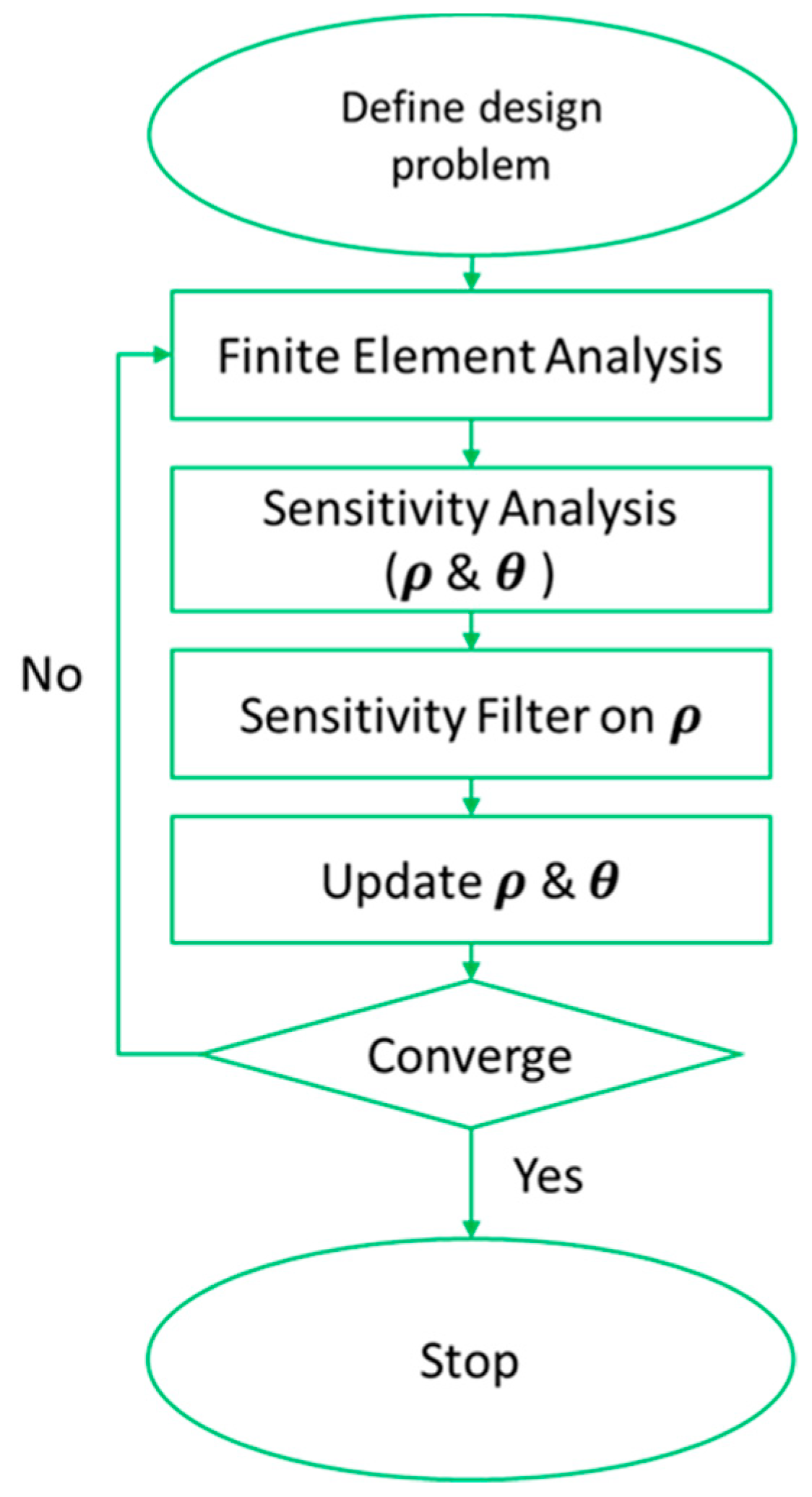
2.4. Optimization Process

Figure 2 illustrates the iterative topology optimization process used in our work. Firstly, the design domain and boundary conditions are defined, and the domain is discretized into quadrilateral elements in 2D or hexagonal elements in 3D. Secondly, the finite element analysis (FEA) procedure is performed to calculate the global displacement vector U by solving KU = F in Equation (2) where two-point Gauss quadrature (i.e., n_gp = 2) is used for the numerical integrations appearing in Equations (3) and (8). Thirdly, the compliance objective function in Equation (4) and its design sensitivities in Equations (7) and (8) are computed on an element-by-element basis where we use a penalization power of p = 3 and $r_{\min }$ is assigned a value of 1.5. Fourthly, the design sensitivities with respect to the density variables are filtered using a linear weighted-average function appearing in Equations (9) and (10). Fifthly, the objective function and design sensitivities are used by the Matlab optimizer function fmincon [53] to update the design variable vectors $\mathsf{\rho }$ and $\mathsf{\theta }$. During the iteration process, the allowable range for density variables is from ${\rho }_{\min }=$ ${10}^{-6}$ to 1. The complete finite element, design sensitivity analysis, and optimization process was performed in our custom Matlab code. To the best of our knowledge, there is no commercially available program for simultaneously computing optimal topology and material orientation for microstructures such as those produced in the FFF process.

The default Matlab fmincon solver interior-point algorithm was chosen as the optimization scheme in our examples where the optimal constrained nonlinear problem is solved by introducing an exterior barrier function into the objective function. A convergence criterion is defined to end computations when relative changes of design variables and objective function values between two iterations are smaller than 0.1%. Our use of Matlab nonlinear programming methods provides a more general approach for incorporating both material angle and density design variables into the topology optimization problem than is afforded by typical density-only approaches [4,32]. To reduce computational time for our topology optimizations, we used the parallel processing capabilities of Matlab when calculating the element stiffness matrices and solving the linear system of equations in our finite element analyses.

While optimality criteria-based methods enjoy extensive application in the topology optimization literature (see, e.g., development of the homogenization method and SIMP method described in Bendsøe and Sigmund [4]), little attention has been given to its use for determining optimal material orientations outside of homogenization method applications. When an optimal material orientation is desired, prior research updated density design variables with Equation (9) (and also Equations (11) and (12)) while computing a constant-density sub-optimal material orientation at each density iteration as in Soto and Yang [54,55]. It is expected that computational efficiencies could be gained through a study of minimization algorithms for our material density and orientation AM design approach; however, our focus here was firstly obtaining useful results for parts produced by AM.

3. CFAO Design Examples

Numerical examples are presented below to illustrate our CFAO topology optimization methodology. The first example considers a 2D print domain for a center-loaded simply supported beam where all loading is within the plane and all FFF layers are assumed to be printed in the same manner. Following this example, we present the static load testing of a structures printed to follow the 2D CFAO topology results. Finally, the second numerical example considers a 3D cantilever beam which is optimized for printing in each of three different directions. The study aims to quantify the effect of print direction on the elastic response of the optimized printed part. Additional examples that demonstrate the optimization procedure and the code may be found in Hoglund [56] and also Jiang [57].

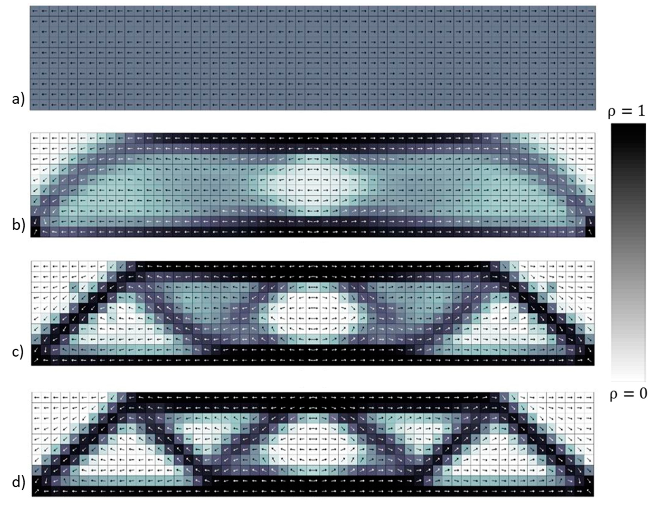
3.1. One-Dimensional (1D) CFAO Topology Optimization Example

To illustrate the applicability of the CFAO method to polymer composite FFF part design, a 2D topology optimization was considered here first based on the Messerschimitt–Bölkow–Blohm (MBB) beam (see, e.g., Bendsøe and Kikuchi [28]). The MBB beam is defined by the design domain appearing in Figure 3 where the topology optimization is expected to produce a truss-like structure as in prior topology optimization studies. In this example, the elastic modulus in the fiber direction was set to 5 units while the elastic modulus normal to the fiber direction was 1 unit. Poisson’s ratio of the major direction (greater Young’s modulus) was defined to be 0.3. We defined the topology optimization volume fraction constraint in Equation (2) with f = 0.5. In the following analysis, all elements contain both a density and a fiber angle design variable which define the topology optimization problem from Equations (1) and (2) having the number of design variables equal to twice the number of elements. The thickness of the model into the plane was set to h = 1 unit, and the applied load was 1 unit acting downward in the center of the design domain as shown. The topology optimization was performed with a half-symmetry finite element model having 30 elements in the horizontal direction and 10 elements in the vertical direction where each element was 1 unit by 1 unit square (note that results from the half-symmetry model are mirrored in Figure 4 to show the entire structure for better illustration).

Selected designs taken from iterations of the CFAO topology optimization appear in Figure 4. Elements in the figure appear dark as ${\rho }_e$ approaches unity (i.e., element full of material), and white as ${\rho }_e$ approaches zero (i.e., no material). Also shown in each element is an arrow indicating the fiber angle direction. Note that all ${\theta }_e$ are zero for the initial design and quickly change to become parallel to the direction of the dominant structure in the truss-like members. The topology of the structure emerges after approximately 25 iterations; however, the edge of the truss-like members become more distinct as the optimization concludes.

To better understand the effect of mesh size on the optimal layout and compliance, the topology optimization described above was repeated here using various mesh sizes. All parameters for these optimizations were the same as that given above except that the modulus in the fiber direction was set to 10 units and the Poisson’s ratio of the material was 0.36. The modulus normal to the fiber direction remained at 1 unit as before. We note that, in other work (see, e.g., Hoglund [56]), the optimal topology and fiber direction for the MBB beam was found to be nearly the same once the modulus ratio exceeded about 2 making these result comparable to those given above. Computed optimal topologies and fiber directions appear in Figure 5, and values of optimal compliance, central processing unit (CPU) time, and number of optimization iterations are given in

Table 1. Continuous fiber angle optimization (CFAO) Messerschimitt–Bölkow–Blohm (MBB) optimization results for various mesh sizes. CPU—central processing unit.

Mesh Size	Number of Design Variables	Number of Iterations	CPU Time (s)	Minimum Compliance
60 × 10	1200	78	188	13.6
90 × 15	2700	151	847	11.8
120 × 20	4800	169	2094	12.1
150 × 25	7500	241	6415	12.6
180 × 30	10,800	341	17,681	13.2

.

Computed values in Table 1 show that the compliance of the structure does not decrease with increased mesh density as one might expect. We note that there is no guarantee that the global minimum is achieved here due to the complexity of the nonconvex objective function. The optimization routine may instead converge to a local minimum at higher mesh sizes as opposed to finding the global minimum. The local minimum issue appears in related topology optimizations that also consider material orientation in a similar manner (see, e.g., References [44,58]), and should be addressed in future research in directional topology optimization.

Results in Figure 5 show that, as the mesh size increased, the optimal structure became increasingly complex. Although the sensitivity filter was designed to prevent mesh-dependency in SIMP topology optimizations [41], it may not be effective in preventing a local minimum from occurring in the simultaneous optimization of fiber direction and material distribution, even with implementation of a mesh-independent filter radius. The distribution of material in Figure 5 designs became noticeably different for mesh sizes higher than 120 × 20 mesh. In all cases, optimized fiber directions were aligned along the principal stress directions of the segments. For singly loaded structures, this follows the established theory that the alignment of the fibers should occur along the principal stress directions of the structure [59]. As expected, the number of optimization iterations and CPU time, shown in Table 1 (CPU time reported for an Intel i7-4930K CPU at 3.4 GHz and 64 GB random-access memory (RAM)), increased with mesh size and the number of design variables.

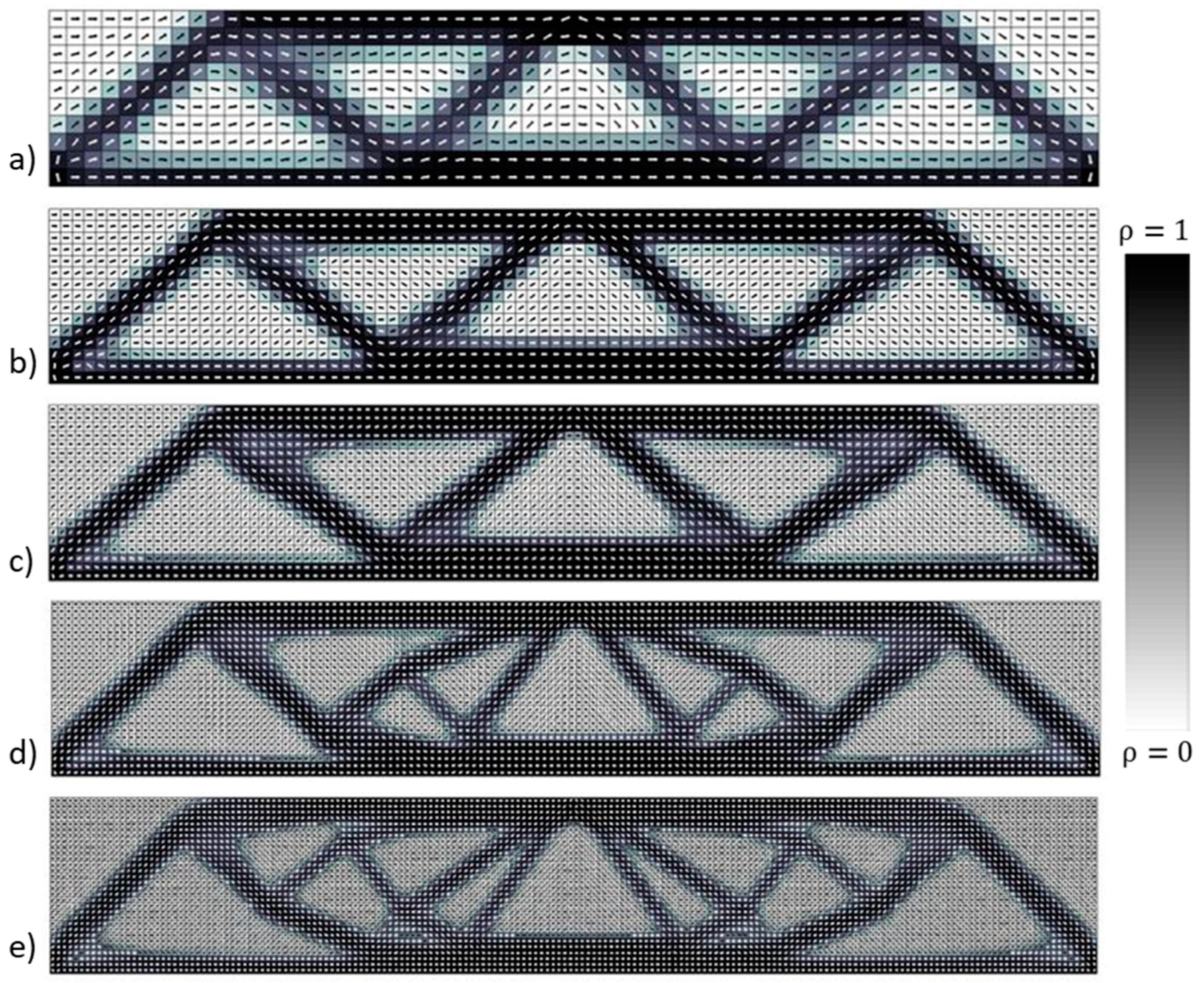
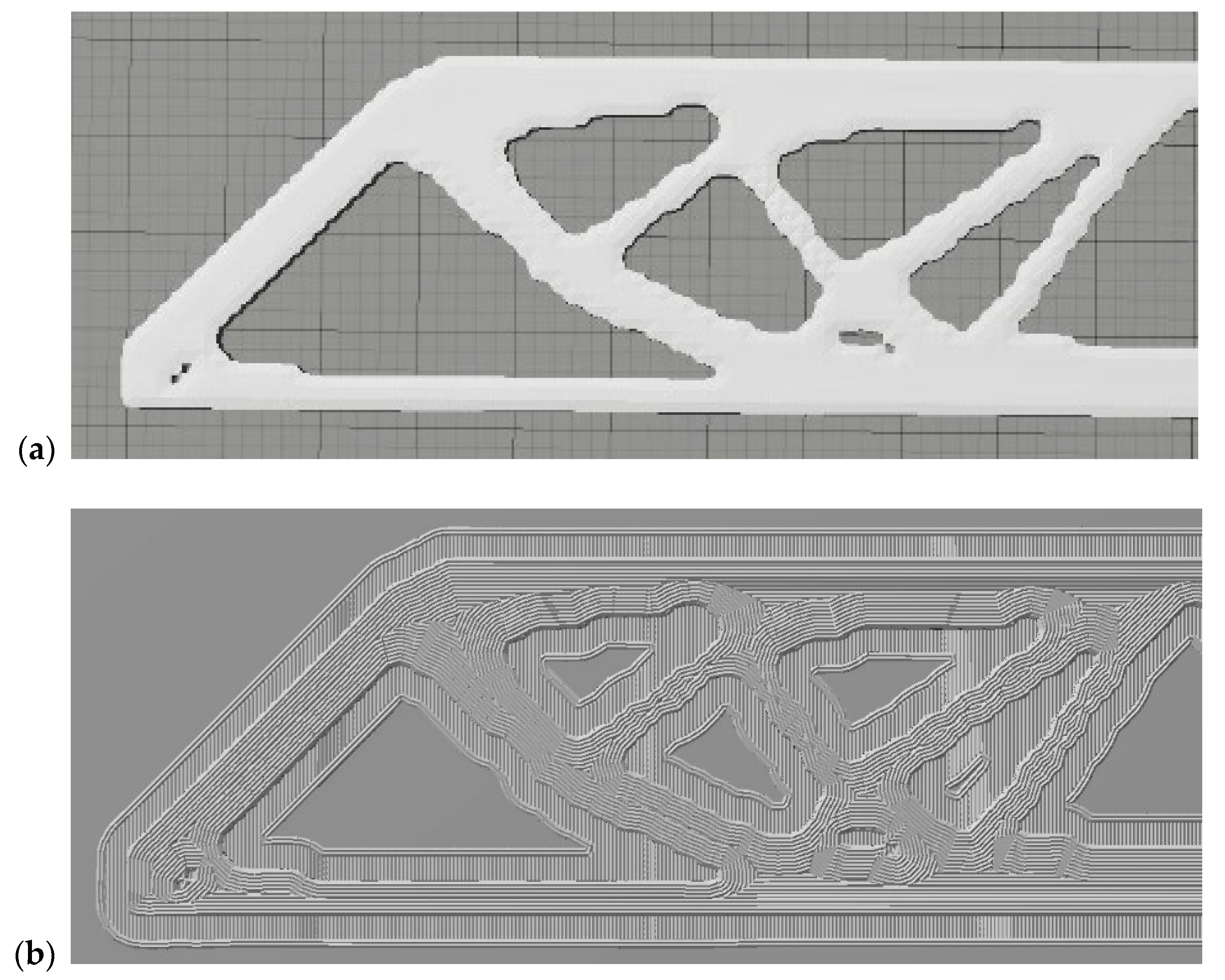
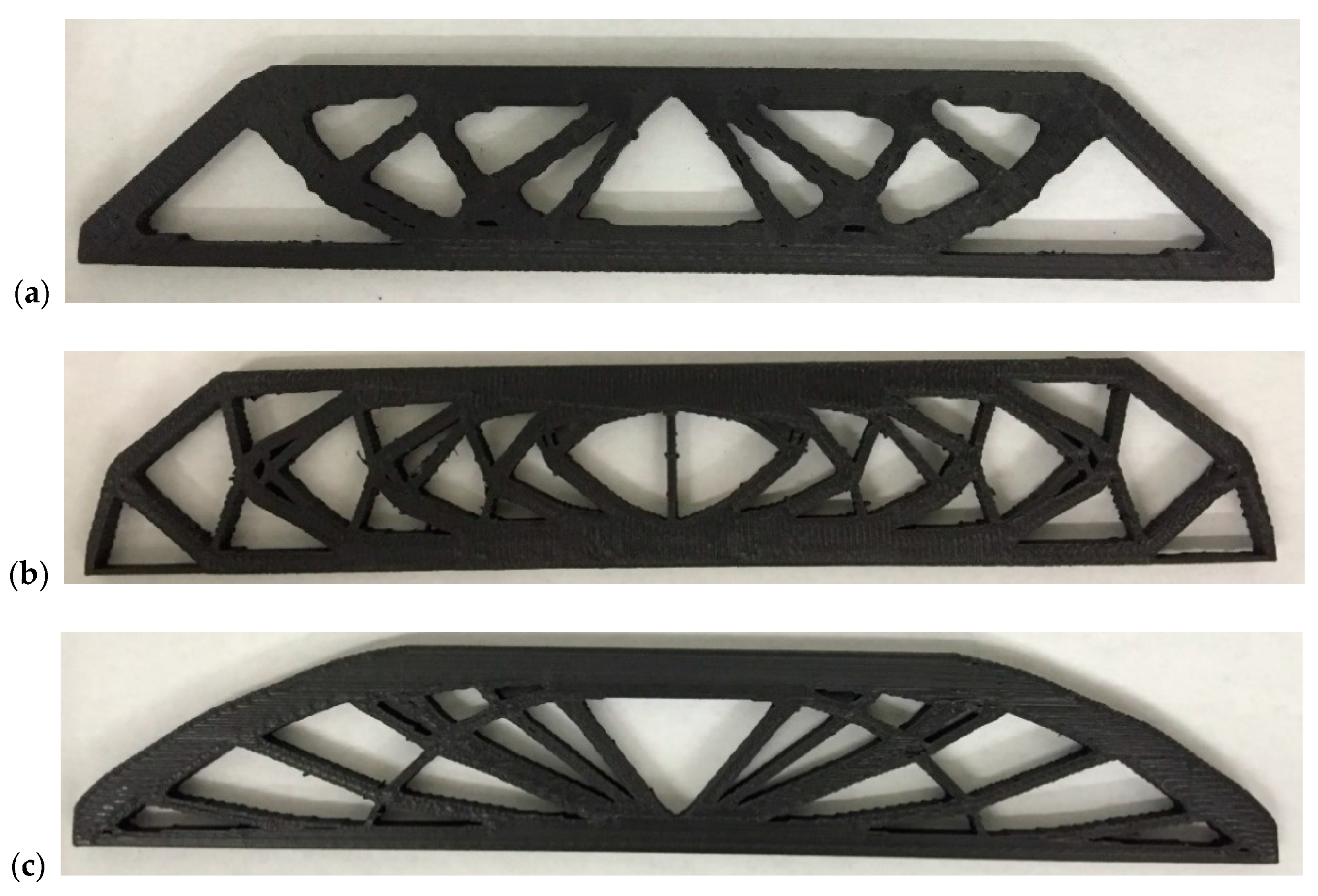
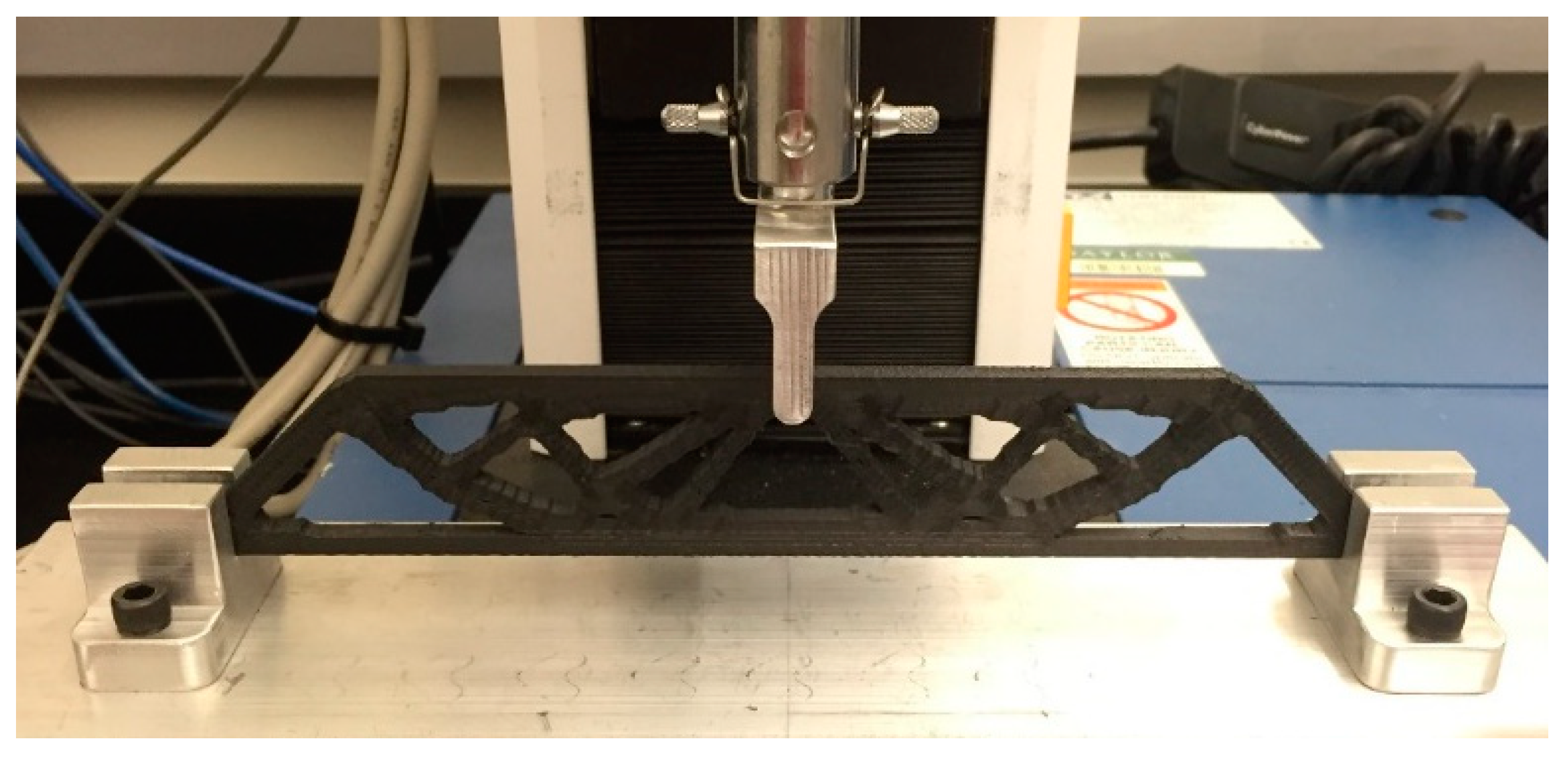
3.2. 2D CFAO Beam Experimental Verification of Computed Results

To further demonstrate the effectiveness of the CFAO method, optimized MBB beams from Section 3.1 were printed with varying fiber orientations using carbon-fiber-reinforced polylactic acid (PLA) marketed as 3DXMax CFR-PLA by 3DxTECH (3DXTECH, Byron Center, MI, USA). The filament contained approximately 15% carbon fiber by weight (with measured weight-averaged fiber length and aspect ratio of 72.8 μm and 9.4, respectively) in a 1.77-mm-diameter filament and had a published tensile strength of 47.9 MPa and a tensile modulus of 4.791 GPa. Our MBB beam structures were printed with a MakerBot Replicator 2.0 3D FFF printer with a hardened steel 0.6-mm-diameter nozzle. Nozzle temperature during printing was 220 °C and print bed heating was not used. Characterization of the same CFR-PLA including fiber length distribution, tensile strength for various print orientations, and micro structural analysis may be found in Jiang and Smith [19]. The geometry of the printed MBB beams was taken from the optimized result appearing in Figure 5e. The FFF structures were printed with 100% infill to reduce interbead voids within the material, and the 2D topologies were printed with a total part thickness of 5.5 mm with multiple identical layers having a thickness of 0.2 mm. We note that other CFR filaments such as CFR-ABS could have been used in this work; however, CRF-PLA is easier to print and provides the necessary structural attributes for verifying our topology results.

To produce a printable format of the topology optimizations, the code Top3dSTL_v3.m was used to convert the physical array of elemental densities to stl file format [60]. We used Top3dSTL_v3.m to translate the optimal density distributions to an STL file where each element represents a unit cube. The two-dimensional information for the planar MBB beam was retained while the thickness out-of-plane is modified to adjust for scaling of the part dimensions in the plane. Autodesk MeshMixer (AutoDesk, San Rafael, CA, USA) was used to smooth the edges of the CFAO structures prior to printing. This smoothing helped facilitate a printed part that had beads such as those appearing in Figure 6 with a primary orientation parallel to the edge of the truss-like members that resulted from the CFAO optimizations. To realize print paths that remained mostly parallel to the edge of the structure, a contour-parallel deposition strategy was employed. In this case, the strategy was implemented by specifying a high number of shell layers in the MakerBot Desktop software to ensure that all printed beads approximately aligned with the edges, particularly within the structural members that formed. Higher-quality print beads would likely result by developing more advanced methods for translating topology fiber angle to print path data; however, the method employed here proved sufficient for comparing the CFAO results to other optimal topologies. Figure 6 shows the model data (left half of beam only) at various stages during the processing of data for printing which includes the CFAO optimized topology and fiber angle, the smoothed image obtained with Autodesk MeshMixer, and the bead pattern print path as specified by the MakerBot Desktop. The resulting printed beam appears in Figure 7a. Figure 7b,c show similar optimized beams where the print direction was constrained to only horizontal and only vertical, respectively, as described elsewhere [45].

Printed CFAO optimized MBB beams were tested in three-point bending as shown in Figure 8 using an Instron (Instron, Norwood, MA, USA) tensile test machine with a 2-kN load cell. The load was applied to the top center of the printed beam in the same manner as that used in the CFAO optimization. The structural stiffness was computed from force and displacement data that were collected using the Bluehill 3 (Instron, Norwood, MA, USA) software. Loading was performed in the linear force–displacement range for the sample and testing was ended prior to sample failure.

Three samples of each of the three topologies in Figure 7 were printed and tested to obtain the stiffness results given in

Table 2. Measured stiffness (average of three samples each) of printed CFAO optimized beams with other horizontal (${\theta }_e=0$) and vertical (${\theta }_e$ = 90°) beams (cf. Reference [45]) included for comparison.

MBB Sample	Average Stiffness (N/m)	Standard Deviation (N/m)	Coefficient of Variation
Horizontal bead [45]	2.90 × 105	0.12 × 105	0.042
Vertical bead [45]	2.51 × 105	0.052 × 105	0.021
CFAO	3.26 × 105	0.015 × 105	0.0047

. Also shown in Table 2 are results from similar tests (three samples each) where optimal topologies were computed assuming a fixed horizontal bead path (i.e., ${\theta }_e=0$) and a fixed vertical bead path (i.e., ${\theta }_e$ = 90°) that appear in Figure 7b,c, respectively, as described in Reference [45]. Note that, in these structures with a fixed fiber angle, each element has a single density design variable, which simplifies the calculations and the process for creating the print file. The fixed angle optimizations provide a point of comparison to illustrate the effectiveness of the CFAO method. As shown in Table 2, samples optimized and printed with a horizontal bead were 15.5% stiffer than samples optimized and printed with a predominant vertical bead. This result is to be expected since horizontal stiffening is more efficient than vertical stiffening under the given bending load. Table 2 also shows that CFAO optimized MBB beams performed better than either horizontal or vertical optimized and printed beams. It is seen that the CFAO beam was 29.9% stiffer than the vertical optimized and printed structure and 12.4% stiffer than the horizontal optimized and printed structure. More information on details of the optimization and testing may be found in Hoglund [56].

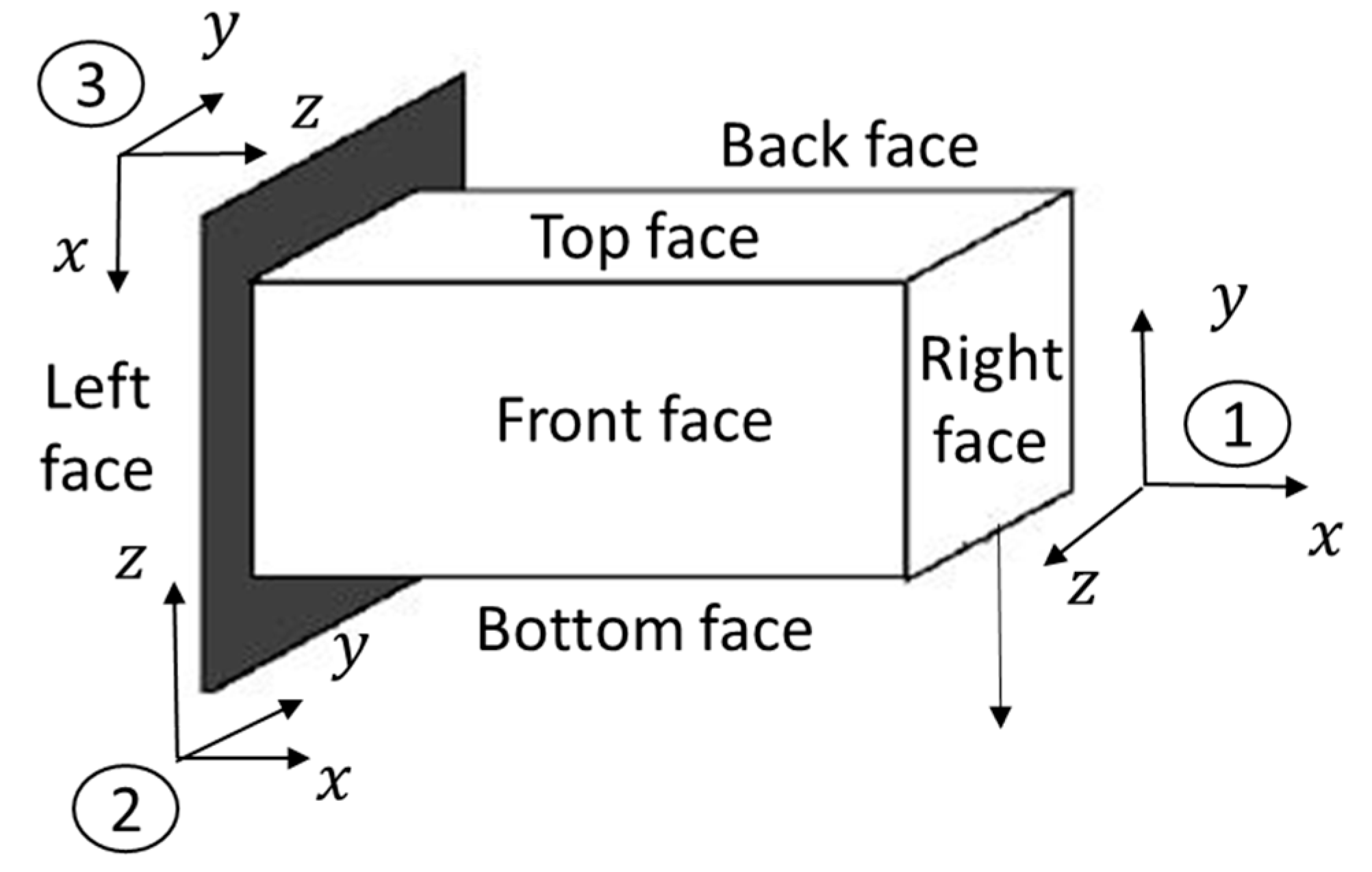
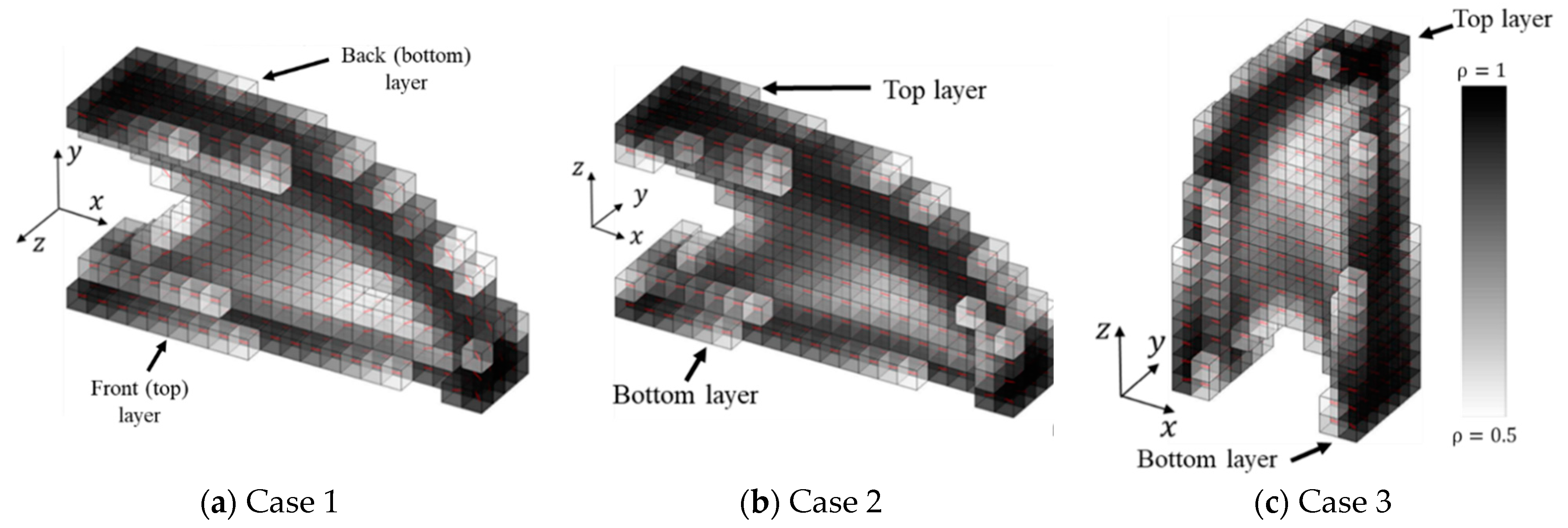
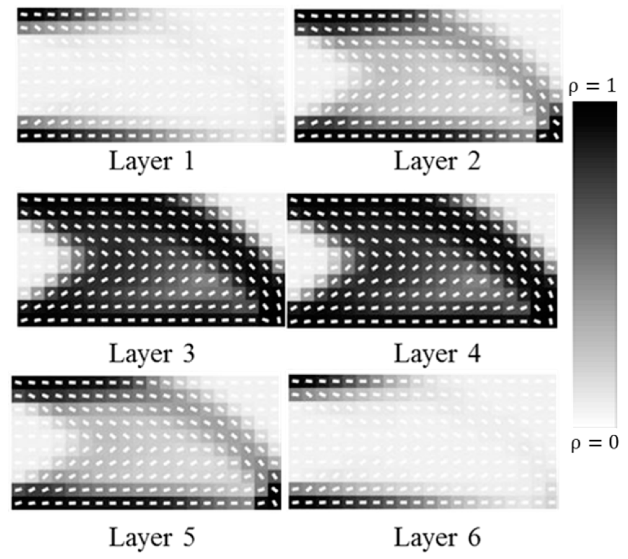
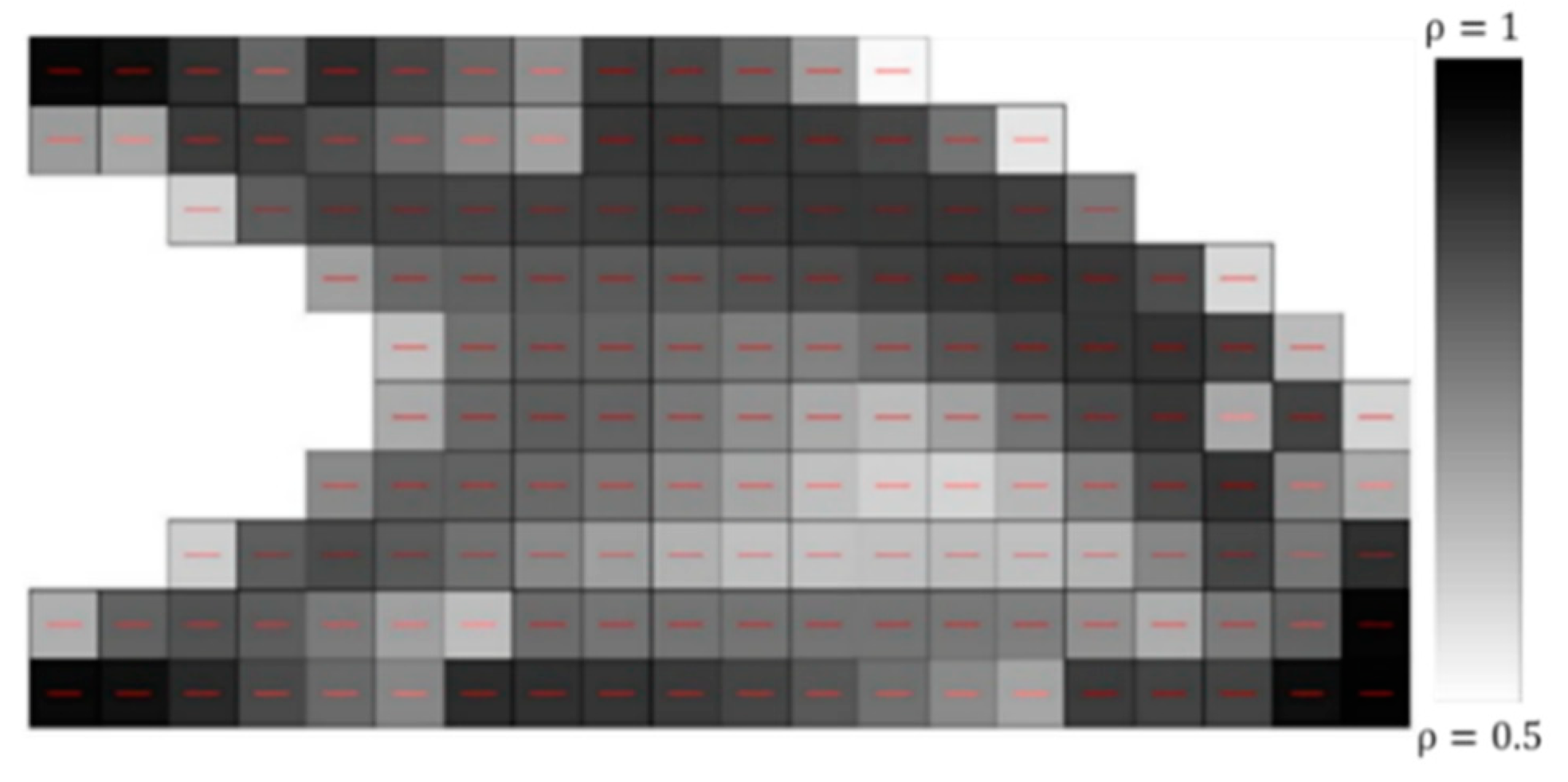
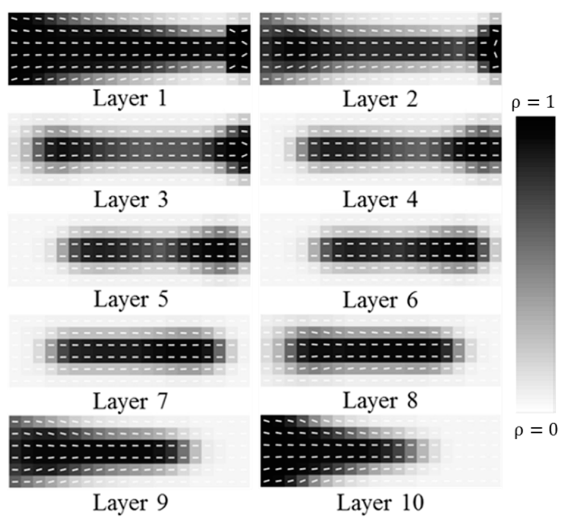
3.3. 3D CFAO Topology Optimization Example

In the 3D example problems presented here, material constants in Equation (6) were taken from the work by Heller et al. [25], who presented a computational method for predicting fiber orientation in a FFF nozzle. They investigated how die-swell affects fiber orientation and the polymer composite non-isotropic elastic properties after the fiber-filled polymer composite emerges from the nozzle during printing. Therefore, the elastic properties of the polymer composites within the extrudate swell region from Heller were used for constructing the C matrix in Equation (6) for our work. The examples below are based on FFF polymer composite filament having 15% fiber volume, with $E_f=240\mathrm{GPa}$, $v_f=0.2$, $E_m=2\mathrm{GPa}$, and $v_m=0.4$. The aspect ratio of the fiber was 15. These composite material properties were used with fiber orientation data from Heller et al. [25] to obtain the bead elastic constants appearing in

Table 3. Elastic properties from the extrudate swell region [25].

${\mathit{E}}_{\mathit{x}}\left(\mathbf{GPa}\right)$	${\mathit{E}}_{\mathit{y}}\left(\mathbf{GPa}\right)$	${\mathit{G}}_{\mathit{x}\mathit{y}}\left(\mathbf{GPa}\right)$	${\mathit{\upsilon }}_{\mathit{x}\mathit{y}}$	${\mathit{\upsilon }}_{\mathit{y}\mathit{z}}$
7.34	3.43	1.39	0.42	0.47

where the x-direction was along the axis of the bead (i.e., fiber direction in the topology optimization), and the y-direction was normal to the bead axis.

The three-dimensional example considered here was a cantilever beam with a unit load applied to its tip as shown in Figure 9. Topology optimizations were performed for each of three different print planes defined by the three sets of xy Cartesian planes appearing in Figure 9. The topology optimization was first performed assuming that AM deposition occurred from the back to the front face (labeled Case 1). A second optimization was then performed assuming that printing was done from the bottom to the top face (labeled Case 2). Finally, a third separate optimization was performed assuming that printing occurred from the left to right face (labeled Case 3). The definition of the density design variables for these optimizations was the same; however, the axis about which the material direction design variable ${\theta }_e$ was defined differed for each problem. It is well understood that the elastic response of a structure is significantly affected by print orientation. The examples shown here not only quantify the difference, but also demonstrate how print direction influences the optimal topology and optimal bead direction of a 3D printed structure.

The finite elements in these optimizations were hexahedral having a size of 1 m × 1 m × 1 m. The finite element model used in the topology optimizations for Cases 1, 2, and 3 had 20 × 10 × 6, 20 × 6 × 10, and 10 × 6 × 20 elements (i.e., length × width × height), respectively, yielding a total of 2400 design variables (1200 density and 1200 material angle design variables) for each optimization problem. A volume fraction of $f=0.4$ was assigned for the volume constraint in all optimizations, and the initial densities and material angles were assigned $0.4$ and 0 radians, respectively, where the all element material angles ${\theta }_e$ were measured in the xy plane as positive counter-clockwise from the positive x-axis. Loading and boundary conditions were the same for all three optimizations.

Figure 10, Figure 11, Figure 12, Figure 13, Figure 14, Figure 15 and Figure 16 show the optimized topology and element material angles computed for each of the three print plane directions described above. Output is presented in isometric, top, and front views. Figure 10 shows the isometric perspectives of the optimization result for Case 1, Case 2, and Case 3, printed in each of the directions shown in Figure 9. The optimal structures for all optimizations formed a shape in the form of an I-beam regardless of the print direction. In all cases, material was redistributed to the wider sides of the I-beam shape during the optimization, as indicated by the higher density (i.e., darker color) in each figure. This extra material gave the I-beam the needed stiffness to support the bending load.

In addition to the 3D isometric plots, the optimized structure appears in a view that is orthogonal to the print plane to better illustrate the material distribution and material angle for each layer of the structure. Figure 11 and Figure 12 show each layer of material distribution and material angle for Case 1. In Figure 11, the material angles all appear horizontal as expected since the view is sideways into the print plane. The optimal result was symmetric about the beam’s mid plane which was expected since the load was applied at the center of the right bottom edge, as shown in Figure 9. It is clear from Figure 12 that density and material angle appeared to be the same for layers 1 and 6, layers 2 and 5, and layers 3 and 4. Material angle plots in Figure 12 show that the optimal material orientation followed the outer contour of the structure for each layer where the dense material was distributed, which is very similar to 2D results given above and by Nomura et al. [44].

Figure 13 shows the front view of the optimized shape including the optimal layout of the structure and the orientation of the material angle for Case 2. Figure 14 shows a layer-by-layer plot for the material distribution and material angle for the Case 2 optimal result. Note that the direction of material angle tended to point toward the applied load, which was expected as the structure was modified during the optimization to support the tip load carried by the beam.

Figure 15 shows the front view of the optimized shape for the Case 3 optimization. Again, a cantilever beam structure was revealed as before. Figure 16 shows the material distribution and material orientation for each layer, where layer 1 is at the bottom and layer 20 at the top of the optimized structure. Fiber orientation symmetry existed in each layer by comparing the first three layers counting from the top to the three layers counting from the bottom.

Table 4. Topology result comparisons between Case 1, Case 2, and Case 3.

Case Study	Initial Compliance (Nm)	CPU Time (s)	Iterations	Optimized Compliance (Nm)
Case 1	30.27	246.3	78	3.48
Case 2	30.27	165.5	54	4.28
Case 3	37.86	144.2	47	5.66

presents the initial design compliance for each case, and provides output to compare the CPU time, the number of iterations, and the compliance for the three topology optimization cases presented above. All cases had dramatic improvement in stiffness design after the optimization process. The CPU time required to solve Case 1 was 48.8% and 70.8% more than Case 2 and Case 3, respectively. Similarly, Case 1 required 24 and 31 more optimization iterations than Cases 2 and 3, respectively. Case 1 yielded 23% and 63% lower optimal compliance than Case 2 and Case 3, respectively. In Case 1, material angle design variables allowed the preferred material direction to rotate in a plane that had a larger effect on the structure’s minimum compliance. However, for Case 2 and Case 3, the plane of material angle was normal to the direction of the force, resulting in an optimization that yielded less improvement in terms of the compliance. These results show that the relationship between the applied loads and print plane orientation has a significant effect on the outcome of the topology optimization.

4. Conclusions

This paper presented a topology optimization approach for non-isotropic microstructures produced with fiber-filled polymer composite AM techniques. Special attention was given to the unique properties for material orientation offered by AM as it relates to the layer-by-layer process of building structures. Our approach enhances the traditional SIMP approach by including fiber angle as a design variable and using the Matlab fmincon optimization tool to solve 2D and 3D finite-element-based topology optimization design problems. We considered the common topology optimization design problem of compliance minimization with a constraint on material usage. Design sensitivities were obtained using the adjoint variable method, and a sensitivity filter was implemented to avoid checkerboarding. Our optimization scheme was shown to compute design with oriented microstructures for planar problems and also more general 3D domains. In addition, a procedure was described to physically realize the optimized 2D planar structures. Static load testing showed that structures obtained using our CFAO technique performed better than those derived from a sub-optimal design space. The 3D example problems illustrated the significant difference in minimum compliance that can be obtained based on print direction. It was also shown that the case where the plane of material alignment was parallel with force direction gave the lowest compliance. Furthermore, printing the structure at different plane directions gave very different compliance results, which is important for designers when considering the potential loading scenarios. In our example, the minimum compliance was reduced by 63% by selecting a different print orientation. Finally, fiber orientation generally followed the outer contour of the dense material region for each layer. This work offers a starting point for future work on topology optimization with AM structures. Extending the design space to include more general shapes should be done, as well as incorporating print deformation into the topology optimization process. The addition of stress-based constraints and optimal support structures would also be valuable extensions of the work presented here.

References

1. Ahn, S.H.; Montero, M.; Odell, D.; Roundy, S.; Wright, P.K. Anisotropic Material Properties of Fused Deposition Modeling ABS. Rapid Prototyp. J. 2002, 8, 248–257. [Google Scholar] [CrossRef]
2. Bagsik, A.; Schöppner, V. Mechanical Properties of Fused Deposition Modeling Parts Manufactured with ULTEM* 9085. In Proceedings of the ANTEC 2011, Boston, MA, USA, 1–5 May 2011. [Google Scholar]
3. Ziemian, C.; Sharma, M.; Ziemi, S. Anisotropic Mechanical Properties of ABS Parts Fabricated by Fused Deposition Modelling. In Mechanical Engineering; Gokcek, M., Ed.; InTech Open: London, UK, 2012. [Google Scholar] [Green Version]
4. Bendsøe, M.P.; Sigmund, O. Topology Optimization; Springer: Berlin/Heidelberg, Germany, 2004. [Google Scholar]
5. Sundararajan, V.G. Topology Optimization for Additive Manufacturing of Customized Meso-Structures Using Homogenization and Parametric Smoothing Functions. Ph.D .Thesis, University of Texas at Austin, Austin, TX, USA, 2010. [Google Scholar]
6. Gaynor, A.T.; Meisel, N.A.; Williams, C.B.; Guest, J.K. Multiple-Material Topology Optimization of Compliant Mechanisms Created Via PolyJet Three-Dimensional Printing. J. Manuf. Sci. Eng. 2014, 136, 061015. [Google Scholar] [CrossRef]
7. Wang, X.; Xu, S.; Zhou, S.; Xu, W.; Leary, M.; Choong, P.; Qian, M.; Brandt, M.; Xie, Y.M. Topological Design and Additive Manufacturing of Porous Metals for Bone Scaffolds and Orthopaedic Implants: A Review. Biomaterials 2016, 83, 127–141. [Google Scholar] [CrossRef] [PubMed]
8. Langelaar, M. Topology Optimization of 3D Self-Supporting Structures for Additive Manufacturing. Addit. Manuf. 2016, 12, 60–70. [Google Scholar] [CrossRef]
9. Mass, Y.; Amir, O. Topology Optimization for Additive Manufacturing: Accounting for Overhang Limitations Using a Virtual Skeleton. Addit. Manuf. 2017, 18, 58–73. [Google Scholar] [CrossRef]
10. Zhang, P.; Toman, J.; Yu, Y.; Biyikli, E.; Kirca, M.; Chmielus, M.; To, A.C. Efficient Design-Optimization of Variable-Density Hexagonal Cellular Structure by Additive Manufacturing: Theory and Validation. J. Manuf. Sci. Eng. 2015, 137, 021004. [Google Scholar] [CrossRef]
11. Wohlers, T. Wohlers Report 2016; Wohlers Associates, Inc.: Fort Collins, CO, USA, 2016. [Google Scholar]
12. Perez, A.R.T.; Roberson, D.A.; Wicker, R.B. Fracture Surface Analysis of 3D-Printed Tensile Specimens of Novel ABS-Based Materials. J. Fail. Anal. Prev. 2014, 14, 343–353. [Google Scholar] [CrossRef] [Green Version]
13. Zhong, W.; Li, F.; Zhang, Z.; Song, L.; Li, Z. Short Fiber Reinforced Composites for Fused Deposition Modeling. Mater. Sci. Eng. A 2001, 301, 125–130. [Google Scholar] [CrossRef]
14. Gray, R.W.; Baird, D.G.; Bøhn, J.H. Thermoplastic Composites Reinforced with Long Fiber Thermotropic Liquid Crystalline Polymers for Fused Deposition Modeling. Polym. Compos. 1998, 19, 383–394. [Google Scholar] [CrossRef]
15. Shofner, M.L.; Lozano, K.; Rodríguez-Macías, F.J.; Barrera, E.V. Nanofiber-Reinforced Polymers Prepared by Fused Deposition Modeling. J. Appl. Polym. Sci. 2003, 89, 3081–3090. [Google Scholar] [CrossRef]
16. Hwang, S.; Reyes, E.I.; Moon, K.; Rumpf, R.C.; Kim, N.S. Thermo-Mechanical Characterization of Metal/Polymer Composite Filaments and Printing Parameter Study for Fused Deposition Modeling in the 3D Printing Process. J. Electron. Mater. 2014, 44, 771–777. [Google Scholar] [CrossRef]
17. Dul, S.; Fambri, L.; Pegoretti, A. Fused Deposition Modelling with ABS–Graphene Nanocomposites. Compos. Part Appl. Sci. Manuf. 2016, 85, 181–191. [Google Scholar] [CrossRef]
18. Tekinalp, H.L.; Kunc, V.; Velez-Garcia, G.M.; Duty, C.E.; Love, L.J.; Naskar, A.K.; Blue, C.A.; Ozcan, S. Highly Oriented Carbon Fiber–Polymer Composites via Additive Manufacturing. Compos. Sci. Technol. 2014, 105, 144–150. [Google Scholar] [CrossRef]
19. Jiang, D.; Smith, D.E. Anisotropic Mechanical Properties of Oriented Carbon Fiber Filled Polymer Composites Produced with Fused Filament Fabrication. Addit. Manuf. 2017, 18, 84–94. [Google Scholar] [CrossRef]
20. Ning, F.; Cong, W.; Qiu, J.; Wei, J.; Wang, S. Additive Manufacturing of Carbon Fiber Reinforced Thermoplastic Composites Using Fused Deposition Modeling. Compos. Part B Eng. 2015, 80, 369–378. [Google Scholar] [CrossRef]
21. Love, L.J.; Kunc, V.; Rios, O.; Duty, C.E.; Elliott, A.M.; Post, B.K.; Smith, R.J.; Blue, C.A. The Importance of Carbon Fiber to Polymer Additive Manufacturing. J. Mater. Res. 2014, 29, 1893–1898. [Google Scholar] [CrossRef]
22. Love, L.J. Utility of Big Area Additive Manufacturing (BAAM) for the Rapid Manufacture of Customized Electric Vehicles; ORNL/TM-2014/607; Oak Ridge National Lab. (ORNL): Oak Ridge, TN, USA, 2015. [Google Scholar]
23. Post, B.; Lloyd, P.D.; Lindahl, J.; Lind, R.F.; Love, L.J.; Kunc, V. The Economics of Big Area Addtiive Manufacturing. In Proceedings of the 27th Annual International Solid Freeform Fabrication Symposium, Austin, TX, USA, 8–10 August 2016. [Google Scholar]
24. Spinnie, N.K. Large Scale Fused Deposition Modeling: The Effect of Process Parameters on Bead Geometry. Master’s Thesis, Baylor University, Waco, TX, USA, 2016. [Google Scholar]
25. Heller, B.P.; Smith, D.E.; Jack, D.A. Effects of Extrudate Swell and Nozzle Geometry on Fiber Orientation in Fused Filament Fabrication Nozzle Flow. Addit. Manuf. 2016, 12, 252–264. [Google Scholar] [CrossRef]
26. Wang, Z.; Smith, D.E. Rheology Effects on Predicted Fiber Orientation and Elastic Properties in Large Scale Polymer Composite Additive Manufacturing. J. Compos. Sci. 2018, 2, 10. [Google Scholar] [CrossRef]
27. Suzuki, K.; Kikuchi, N. A Homogenization Method for Shape and Topology Optimization. Comput. Methods Appl. Mech. Eng. 1991, 93, 291–318. [Google Scholar] [CrossRef]
28. Bendsøe, M.P.; Kikuchi, N. Generating Optimal Topologies in Structural Design Using a Homogenization Method. Comput. Methods Appl. Mech. Eng. 1988, 71, 197–224. [Google Scholar] [CrossRef]
29. Bendsøe, M.P. Optimal Shape Design as a Material Distribution Problem. Struct. Optim. 1989, 1, 193–202. [Google Scholar] [CrossRef]
30. Mlejnek, H.P. Some Aspects of the Genesis of Structures. Struct. Optim. 1992, 5, 64–69. [Google Scholar] [CrossRef]
31. Zhou, M.; Rozvany, G.I.N. The COC Algorithm, Part II: Topological, Geometrical and Generalized Shape Optimization. Comput. Methods Appl. Mech. Eng. 1991, 89, 309–336. [Google Scholar] [CrossRef]
32. Sigmund, O. A 99 Line Topology Optimization Code Written in Matlab. Struct. Multidiscip. Optim. 2001, 21, 120–127. [Google Scholar] [CrossRef]
33. Andreassen, E.; Clausen, A.; Schevenels, M.; Lazarov, B.S.; Sigmund, O. Efficient Topology Optimization in MATLAB Using 88 Lines of Code. Struct. Multidiscip. Optim. 2011, 43, 1–16. [Google Scholar] [CrossRef]
34. Liu, K.; Tovar, A. An Efficient 3D Topology Optimization Code Written in Matlab. Struct. Multidiscip. Optim. 2014, 50, 1175–1196. [Google Scholar] [CrossRef]
35. Xie, Y.M.; Steven, G.P. A Simple Evolutionary Procedure for Structural Optimization. Comput. Struct. 1993, 49, 885–896. [Google Scholar] [CrossRef]
36. Tang, Y.; Kurtz, A.; Zhao, Y.F. Bidirectional Evolutionary Structural Optimization (BESO) Based Design Method for Lattice Structure to Be Fabricated by Additive Manufacturing. Comput.-Aided Des. 2015, 69, 91–101. [Google Scholar] [CrossRef]
37. Yang, R.J.; Chuang, C.H. Optimal Topology Design Using Linear Programming. Comput. Struct. 1994, 52, 265–275. [Google Scholar] [CrossRef]
38. Jia, H.P.; Jiang, C.D.; Li, G.P.; Mu, R.Q.; Liu, B.; Jiang, C.B. Topology Optimization of Orthotropic Material Structure. Mater. Sci. Forum. 2008, 575–578, 978–989. [Google Scholar] [CrossRef]
39. Bruyneel, M.; Fleury, C. Composite Structures Optimization Using Sequential Convex Programming. Adv. Eng. Softw. 2002, 33, 697–711. [Google Scholar] [CrossRef]
40. Lindgaard, E.; Lund, E. Optimization Formulations for the Maximum Nonlinear Buckling Load of Composite Structures. Struct. Multidiscip. Optim. 2011, 43, 631–646. [Google Scholar] [CrossRef]
41. Sigmund, O.; Petersson, J. Numerical Instabilities in Topology Optimization: A Survey on Procedures Dealing with Checkerboards, Mesh-Dependencies and Local Minima. Struct. Optim. 1998, 16, 68–75. [Google Scholar] [CrossRef]
42. Sigmund, O. Morphology-Based Black and White Filters for Topology Optimization. Struct. Multidiscip. Optim. 2007, 33, 401–424. [Google Scholar] [CrossRef]
43. Setoodeh, S.; Abdalla, M.M.; Gürdal, Z. Combined Topology and Fiber Path Design of Composite Layers Using Cellular Automata. Struct. Multidiscip. Optim. 2005, 30, 413–421. [Google Scholar] [CrossRef]
44. Nomura, T.; Dede, E.M.; Lee, J.; Yamasaki, S.; Matsumori, T.; Kawamoto, A.; Kikuchi, N. General Topology Optimization Method with Continuous and Discrete Orientation Design Using Isoparametric Projection. Int. J. Numer. Methods Eng. 2015, 101, 571–605. [Google Scholar] [CrossRef]
45. Hoglund, R.; Smith, D.E. Non-Isotropic Material Distribution Topology Optimization for Fused Deposition Modeling Products. In Proceedings of the 26th Annual Solid Freeform Fabrication Symposium, Austin, TX, USA, 12–14 August 2015. [Google Scholar]
46. Hoglund, R.; Smith, D.E. Continuous Fiber Angle Topology Optimization for Polymer Fused Filament Fabrication. In Proceedings of the 27th Annual International Solid Freeform Fabrication Symposium, Austin, TX, USA, 8–10 August 2016. [Google Scholar]
47. Jiang, D.; Smith, D.E. Topology Optimization for 3D Material Distribution and Orientation in Additive Manufaturing. In Proceedings of the 28th Annual International Solid Freeform Fabrication Symposium, Austin, TX, USA, 7–9 August 2017. [Google Scholar]
48. Xia, Q.; Shi, T. Optimization of Composite Structures with Continuous Spatial Variation of Fiber Angle through Shepard Interpolation. Compos. Struct. 2017, 182, 273–282. [Google Scholar] [CrossRef]
49. Huebner, K.H.; Dewhirst, D.L.; Byrom, T.G.; Smith, D.E. The Finite Element Method for Engineers; John Wiley & Sons: Hoboken, NJ, USA, 2001. [Google Scholar]
50. Barbero, E.J. Introduction to Composite Materials Design, 2nd ed.; CRC Press: Boca Raton, FL, USA, 2010. [Google Scholar]
51. Kollár, L.P.; Springer, G.S. Mechanics of Composite Structures; Cambridge University Press: Cambridge, UK, 2003. [Google Scholar]
52. Tortorelli, D.A.; Michaleris, P. Design Sensitivity Analysis: Overview and Review. Inverse Probl. Eng. 1994, 1, 71–105. [Google Scholar] [CrossRef]
53. Find Minimum of Constrained Nonlinear Multivariable Function—MATLAB Fmincon. Available online: https://www.mathworks.com/help/optim/ug/fmincon.html (accessed on 17 December 2016).
54. Soto, C.A.; Yang, R. Optimum Topology of Embossed Ribs in Stamped Plates. In Proceedings of the ASME Design Engineering Technical Conference Proceedings, Atlanta, GA, USA, 13–16 September 1998. [Google Scholar]
55. Soto, C.; Yang, R.-J. Optimum Layout of Embossed Ribs to Maximize Natural Frequencies in Plates. Des. Optim. Int. J. Prod. Process Improv. 1999, 1, 44–54. [Google Scholar]
56. Hoglund, R. An Anisotropic Topology Optimization Method for Carbon Fiber-Reinforced Fused Filament Fabrication. Master’s Thesis, Baylor University, Waco, TX, USA, 2016. [Google Scholar]
57. Jiang, D. Three Dimensional Topology Optimization with Orthotropic Material Orientation Design for Additive Manufacturing Structures. Master’s Thesis, Baylor University, Waco, TX, USA, 2017. [Google Scholar]
58. Stegmann, J.; Lund, E. Discrete Material Optimization of General Composite Shell Structures. Int. J. Numer. Methods Eng. 2005, 62, 2009–2027. [Google Scholar] [CrossRef]
59. Flow-INDUCED Alignment in Composite Materials, 1st ed. Available online: https://www.elsevier.com/books/flow-induced-alignment-in-composite-materials/papthanasiou/978-1-85573-254-4 (accessed on 20 December 2018).
60. Liu, K. Top3dSTL_v3, Top3d: An Efficient 3D Topology Optimization Program. Top3d. Available online: https://top3dapp.com/download-archive/ (accessed on 20 December 2018).
Figure 1. Isoparametric hexahedral element with node number.
Fibers 07 00014 g001
Figure 2. Flow chart for the continuous fiber angle optimization (CFAO) topology optimization process.
Fibers 07 00014 g002
Figure 3. Messerschimitt–Bölkow–Blohm (MBB) beam design space with boundary conditions and applied load.
Fibers 07 00014 g003
Figure 4. CFAO density and fiber angle results for the MBB beam after (a) 0 iterations (i.e., initial design), (b) 5 iterations, (c) 25 iterations, and (d) final iteration 48. Elements with density approaching unity appear dark, while those appearing white indicate zero density.
Fibers 07 00014 g004
Figure 5. CFAO optimization of MBB beam using various mesh sizes: (a) 60 × 10 elements, (b) 90 × 15 elements, (c) 120 × 20 elements, (d) 150 × 25 elements, and (e) 180 × 30 elements.
Fibers 07 00014 g005
Figure 6. CFAO optimized MBB print data (left half only) of the optimized density and fiber angle distribution (5400 element model) in Figure 5e: (a) MeshMixer smoothed STL file data, and (b) MakerBot Desktop print bead pattern.
Fibers 07 00014 g006
Figure 7. Printed optimized MBB beams: (a) CFAO optimized beam from Figure 4, (b) optimized for fixed horizontal print direction ( θ e = 0 ) (Adapted from Reference [45]), and (c) optimized for fixed vertical print direction ( θ e = 90°) (Adapted from Reference [45]).
Fibers 07 00014 g007
Figure 8. Mechanical test set up for CFAO optimized MBB beam.
Fibers 07 00014 g008
Figure 9. Cantilever beam with point load, printed in three different directions.
Fibers 07 00014 g009
Figure 10. Isometric views of optimal element density values for three different print directions: Cases 1, 2, and 3. Elements with ρ e 0.5 are not shown.
Fibers 07 00014 g010
Figure 11. Topology result for Case 1 (top view). Elements with ρ e 0.5 are not shown.
Fibers 07 00014 g011
Figure 12. Optimized material distribution and material angle, layer-by-layer plots for Case 1. Layer 1 corresponds to the back layer, and layer 6 corresponds to the front layer.
Fibers 07 00014 g012
Figure 13. Topology result for Case 2 (front view). Elements with ρ e ≤ 0.5 are not shown.
Fibers 07 00014 g013
Figure 14. Optimized material distribution and material orientation, layer-by-layer plots for Case 2. Layer 1 corresponds to the bottom layer, and layer 10 corresponds to the top layer.
Fibers 07 00014 g014
Figure 15. Topology result for Case 3 (front view). Elements with ρ e ≤ 0.5 are not shown.
Fibers 07 00014 g015
Figure 16. Optimized material distribution and material orientation, layer-by-layer plots for Case 3. Layer 1 corresponds to the bottom layer, and layer 20 corresponds to the top layer.
Fibers 07 00014 g016