Combined Transverse Steel-External FRP Confinement Model for Rectangular Reinforced Concrete Columns

Abstract

Recently, the need to increase the strength of reinforced concrete members has become a subject that civil engineers are interested in tackling. Of the many proposed solutions, fiber-reinforced polymer (FRP) materials have attracted attention due to their superior properties, such as high strength-to-weight ratio, high energy absorption and excellent corrosion resistance. FRP wrapping of concrete columns is done to enhance the ultimate strength due to the confinement effect, which is normally induced by steel ties. The existence of the two confinement systems changes the nature of the problem, thus necessitating specialized nonlinear analysis to obtain the column’s ultimate capacity. Existing research focused on a single confinement system. Furthermore, very limited research on rectangular sections was found in the literature. In this work, a model to estimate the combined behavior of the two systems in rectangular columns is proposed. The calculation of the effective lateral pressure is based on the Lam and Teng model and the Mander model for FRP wraps and steel ties, respectively. The model then generates stress-strain diagrams for both the concrete core and the cover. The model was developed for the analysis in extreme load events, where all possible contributions to the column’s ultimate capacity should be accounted for without any margin of safety. The model was validated against experiments, and the results obtained showed good agreement with almost all of the available experimental data.

1. Introduction

Columns are structural members that are essential to most structures. Columns transfer loads mainly through axial compression. Recently, the need to increase the strength of reinforced concrete columns has become a subject that structural engineers are interested in tackling. Of the many proposed solutions, fiber-reinforced polymer (FRP) material has attracted attention due to its superior properties, such as high strength-to-weight ratio, high energy absorption and excellent corrosion resistance. FRP wrapping of concrete columns is done to enhance the capacity and ductility of the column due to the confinement effect, which is normally induced by steel ties. The analysis of columns under extreme loading events requires accounting for all possible factors that contribute to the column’s ultimate capacity, including the confinement effect. The existence of the two confinement systems changes the nature of the problem, thus necessitating specialized nonlinear analysis to obtain the column capacity. There is a need to develop a less empirical model that predicts the behavior of the combined confinement system in rectangular columns where the lateral pressure is generally different in both directions. A 3D concrete plasticity treatment is made to accommodate various admissible stress paths.

Mirmiran et al. [1] investigated the effect of column parameters on FRP-confined concrete. Samaan et al. [2] presented an empirical model to predict the behavior of concrete columns confined with FRP tubes only. Mirmiran et al. [1] used the same equation for the compressive strength of confined concrete (f_cc) in columns wrapped with FRP. Campione and Miraglia [3] presented an analytical model to predict the behavior of concrete columns confined with FRP only under concentric compression. This model considered only square sections with and without rounded corners. Additionally, Campione and Miraglia [3] considered the determination of the ultimate confined strain in their model. They based their method on the energy balance approach proposed by Mander et al. [4]. They extended the approach to account for the presence of FRP in the section. Pulido et al. [5] presented a simplified model to predict the behavior of concrete columns confined with FRP only subjected to pure axial compression. The model consists of two linear segments that define the stress-strain relationship. The first point is taken to be the origin. The second point is defined at the break point, which corresponds to an axial strain of 0.002. The ultimate point consists of the ultimate confined strength and the ultimate confined strain. The proposed model was derived for rectangular sections with no rounded corners. The model also does not consider the aspect ratio effect. A constant shape factor of 0.75 was provided for all rectangular sections. Lam and Teng [6] presented an empirical model to predict the behavior of concrete columns confined with FRP only under pure axial compression. Assessment performed by the American Concrete Institute (ACI) Committee 440 task group [7] showed that this model was the most reliable for predicting the ultimate compressive strength and strain for circular and rectangular columns. As a result, this model has been adopted by the ACI Committee 440 for use in the ACI440.2R-08 guidelines [8]. This model is presented in detail under the concrete confinement models implemented in this paper.

Restrepol and De Vino [9] presented a model to predict the behavior of concrete columns confined with both transverse steel and FRP. They based the transverse steel confinement part in their model on the model of Mander et al. [4]. Wang and Restrepo [10] clarified that the confining FRP stress (f_f) should be obtained from the constitutive material properties. The model proposed by those authors predicted the confined strength only. No expressions were provided to predict the maximum confined strain or the stress-strain relationship. Chun and Park [11] presented their passive confinement model (PCM) to predict the behavior of concrete columns confined with both transverse steel and FRP. The model considers the change in Poisson’s ratio of the confined concrete. This change will affect the expansion rate of the concrete and, thus, the overall confinement. It should be noted that those authors did not specify what the calculated confinement pressure (f_l) corresponded to in the case of a noncircular section. It appears that the model only considers the confining pressure along the width of the section and ignores the pressure provided by the FRP and transverse steel along the depth of the section. Eid [12] developed a model to predict the stress-strain behavior of concrete confined with both transverse steel and FRP in rectangular sections. The model is an extension of a previous model developed by Eid and Paultre [13] for circular sections. The effective lateral pressure was based on the expression proposed by Sheikh and Uzumeri [14] and Mander et al. [4]. The ultimate confined concrete strength and strain are obtained based on the expressions proposed by Lam and Teng [6]. This model provided expressions for all necessary parameters. However, the interaction of the pressures in the x and y directions is not considered. The direction of the pressure that should be used in the analysis was not specified.

2. Confinement Models for Concrete

In this section, the confinement models that form the basis of the proposed combined model will be presented.

2.1. Mander Model for Concrete Confined with Transverse Steel

Mander et al. [4] developed a stress-strain model for concrete confined with transverse steel. The model can be applied for members under static or dynamic loading that is applied either monotonically or cyclically. The model is based on effective lateral pressures, which can be equal or unequal. This allows the model to accounts for the section’s geometry and, in turn, renders it applicable to both circular and rectangular sections.

Mander et al. based the stress-strain curve on equations suggested by Popovics [15]. The equations are as follows:

$$f_c=\frac{f_{cc}xr}{r-1+x^r}$$

(1)

$$x=\frac{{\mathsf{\epsilon }}_c}{{\mathsf{\epsilon }}_{cc}}$$

(2)

$$r=\frac{E_c}{E_c-E_{sec}}$$

(3)

$$E_{sec}=\frac{f_{cc}}{{\mathsf{\epsilon }}_{cc}}$$

(4)

where f_c = longitudinal compressive concrete stress; f_cc = compressive strength of confined concrete; ε_cc = strain at the compressive strength of confined concrete.

The strain at the compressive strength of confined concrete is obtained according to the following equation suggested by Richart et al. [16]:

$${\mathsf{\epsilon }}_{cc}={\mathsf{\epsilon }}_{co}\left(1+5\left(\frac{f_{cc}}{f_c^{\prime }}-1\right)\right)$$

(5)

where $f_c^{\prime }$= unconfined concrete strength; ε_co = strain corresponding to the unconfined concrete strength.

Figure 1 illustrates the proposed stress-strain model. The confined concrete curve illustrates the behavior under concentric axial loading. The ascending branch has an initial slope equal to the modulus of elasticity of concrete (E_c) that decreases as the stress increases until the stress reaches its peak at the confined compressive strength (f_cc). The slope becomes negative, and the stress decreases until the occurrence of the first hoop fracture. The descending branch represents the ductile region of the curve.

Figure 1. Stress-strain model proposed for concrete confined with steel ties.

Figure 1. Stress-strain model proposed for concrete confined with steel ties.

As stated earlier, effective lateral pressures were employed in this model. This approach was similar to the one used by Sheikh and Uzumeri [14]. Arching action leads to the development of portions of concrete in which confining stress is fully developed. Only on these portions can the maximum transverse pressure from the confining steel be exerted effectively. The area of the confined concrete is assumed to be the area within the centerlines of the perimeter hoop (A_cc). Figure 2 shows the effective confinement regions in rectangular sections. It is assumed that the arching action acts in the form of parabolas with an initial slope of 45°. This action occurs vertically between the transverse steel layers and horizontally between longitudinal bars.

Figure 2. Effectively-confined core for rectangular hoop.

Figure 2. Effectively-confined core for rectangular hoop.

Figure 2 above shows that the effective confined area is smaller than the core area; thus, the effective lateral pressure ($f_l^{\prime }$) is obtained as a percentage of the lateral pressure from the transverse reinforcement ($f_l$) as follows:

$$f_l^{\prime }=k_e{f}_l$$

(6)

$$k_e=\frac{A_e}{A_{cc}}$$

(7)

$$A_{cc}=A_c\left(1-{\mathsf{\rho }}_{cc}\right)=\text{area of concrete core}$$

(8)

where k_e = confinement effectiveness coefficient; A_e = area of effectively confined concrete core; ρ_cc = ratio of longitudinal steel to the area of the core.

The effectively confined core area is obtained by deducting the area of the horizontal and vertical parabolas shown in Figure 2. The effective area (A_e) is obtained as follows:

$$A_e=\left(b_c{d}_c-{\displaystyle \sum }_{i=1}^n\frac{{(w_i^{\prime })}^2}{6}\right)\left(1-\frac{s^{\prime }}{2b_c}\right)\left(1-\frac{s^{\prime }}{2d_c}\right)$$

(9)

where $w_i^{\prime }$ = ith clear distance between adjacent longitudinal bars; n = number of longitudinal bars.

Substituting back in the equation for the confinement effectiveness coefficient, the following equation is obtained:

$$k_e=\frac{\left(1-{{\displaystyle \sum }}_{i=1}^n\frac{{(w_i^{\prime })}^2}{6b_c{d}_c}\right)\left(1-\frac{s^{\prime }}{2b_c}\right)\left(1-\frac{s^{\prime }}{2d_c}\right)}{\left(1-{\rho }_{cc}\right)}$$

(10)

The steel ratios in each transverse direction are obtained as follows:

$${\mathsf{\rho }}_x=\frac{A_{sx}}{s{d}_c}$$

(11)

$${\mathsf{\rho }}_y=\frac{A_{sy}}{s{b}_c}$$

(12)

Next, the lateral confining pressures are obtained by:

$$f_{lx}={\mathsf{\rho }}_x{f}_{yh}$$

(13)

$$f_{ly}={\mathsf{\rho }}_y{f}_{yh}$$

(14)

Finally, the effective pressures are obtained as follows:

$$f_{lx}^{\prime }=k_e{\mathsf{\rho }}_x{f}_{yh}$$

(15)

$$f_{ly}^{\prime }=k_e{\mathsf{\rho }}_y{f}_{yh}$$

(16)

For strength determination, the constitutive model proposed by Willam and Warnke [17] is used. Further details are provided in the Formulations Section.

Finally, for the determination of the ultimate confined strain, Scott et al. [18] proposed to set it at the point at which first hoop fracture occurs. This is the point when the lateral pressure is provided by the steel drops and in turn is the end of the meaningful region of the confined curve. Mander et al. [19] proposed an energy balance approach to predict the ultimate confined strain. This is done by equating the ultimate strain energy capacity of the confining reinforcement per unit volume of concrete core (U_sh) to the difference in area between the confined (U_cc) and the unconfined (U_co) concrete stress-strain curves, in addition to the energy required to maintain the yielding of the longitudinal steel (U_sc). This is expressed in the following equation:

$$U_{sh}=U_{cc}+U_{sc}-U_{co}$$

(17)

Below are the expressions for each energy term. All equations are provided in SI units. The expressions for U_sh and U_co were estimated from experiments by Mander et al.:

$$U_{sh}={\mathsf{\rho }}_s{A}_{cc}{{\displaystyle \int }}_0^{{\mathsf{\epsilon }}_{sf}}{f}_{s}d{\mathsf{\epsilon }}_s={\mathsf{\rho }}_s{A}_{cc}·110 \text{MJ}/{\mathrm{m}}^3$$

(18)

$$U_{cc}=A_{cc}{{\displaystyle \int }}_0^{{\mathsf{\epsilon }}_{cu}}{f}_{c}d{\mathsf{\epsilon }}_c{U}_{sc}={\mathsf{\rho }}_{cc}{A}_{cc}{{\displaystyle \int }}_0^{{\mathsf{\epsilon }}_{cu}}{f}_{sl}d{\mathsf{\epsilon }}_c{U}_{co}=A_{cc}{{\displaystyle \int }}_0^{{\mathsf{\epsilon }}_{sp}}{f}_{c}d{\mathsf{\epsilon }}_c=0.017\sqrt{f_{co}^{\prime }} \text{MJ}/{\mathrm{m}}^3$$

(19)

Substituting back in the first equation, it simplifies to:

$$110{ \mathsf{\rho }}_s={{\displaystyle \int }}_0^{{\mathsf{\epsilon }}_{cu}}{f}_{c}d{\mathsf{\epsilon }}_c+{{\displaystyle \int }}_0^{{\mathsf{\epsilon }}_{cu}}{f}_{sl}d{\mathsf{\epsilon }}_c-0.017\sqrt{f_{co}^{\prime }} \text{MJ}/{\mathrm{m}}^3$$

(20)

2.2. Lam and Teng Model for Concrete Confined with FRP Wraps

Lam and Teng [6] developed a stress-strain model for concrete confined with fiber-reinforced polymer (FRP) wraps. Assessment performed by an ACI Committee 440 task group [7] showed that this model was the most reliable for predicting the ultimate compressive strength and strain for circular and rectangular columns. The equations for this model are as follows:

$$f_c=\{\begin{array}{c}{E}_c{\mathsf{\epsilon }}_c-\frac{{\left(E_c-E_2\right)}^2}{4f_c^{\prime }}{\mathsf{\epsilon }}_c^2, \text{for} 0\le {\mathsf{\epsilon }}_c\le {\mathsf{\epsilon }}_t^{\prime }\\ f_c^{\prime }+E_2{\mathsf{\epsilon }}_c,{ \text{for}\mathsf{\epsilon }}_t^{\prime }\le {\mathsf{\epsilon }}_c\le {\mathsf{\epsilon }}_{ccu}\end{array}$$

(21)

$$E_2=\frac{f_{cc}-f_c^{\prime }}{{\mathsf{\epsilon }}_{ccu}}$$

(22)

$${\mathsf{\epsilon }}_t^{\prime }=\frac{2f_c^{\prime }}{E_c-E_2}$$

(23)

Figure 3 illustrates the Lam and Teng stress-strain model. The upper curve illustrates the behavior under concentric axial loading. The first branch is parabolic, and its initial slope equals the modulus of elasticity of concrete (E_c). The second branch is linear and starts at the transition strain (${\epsilon }_t^{\prime }$) calculated above. The curve is continuous at the transition point, as there is no sudden change in the slope there. This behavior has been observed under sufficient FRP confinement. For that to hold, Lam and Teng [6] set a minimum confinement ratio limit ($f_{lf}/f_c^{\prime }$) of 0.07, while the ACI Committee 440 [8] increased it to 0.08. Spoelstra and Monti [20] were able to verify this limit for circular sections in their analytical model. In this work, the limit was taken to be 0.08. If the confinement ratio is below the limit, the Mander model (descending second branch) is used instead.

Figure 3. Stress-strain model for concrete confined with FRP.

Figure 3. Stress-strain model for concrete confined with FRP.

As for the ultimate axial strength and strain, Lam and Teng proposed the following equations:

$$f_{cc}=f_c^{\prime }+{\mathsf{\psi }}_{f}3.3{\kappa }_a{f}_l$$

(24)

$${\mathsf{\epsilon }}_{ccu}={\mathsf{\epsilon }}_c^{\prime }\left(A+12k_b\frac{f_l}{f_c^{\prime }}{\left(\frac{{\mathsf{\epsilon }}_{fe}}{{\mathsf{\epsilon }}_c^{\prime }}\right)}^{0.45}\right)\le 0.01$$

(25)

$\text{where} {\psi }_f=\{\begin{array}{c}1\left(\text{Lam and Teng}\right)\\ 0.95\left(\text{ACI} 440.2R-08\right)\end{array}{\kappa }_a=\frac{A_e}{A_c}{\left(\frac{b}{h}\right)}^2;{\kappa }_b=\frac{A_e}{A_c}{\left(\frac{h}{b}\right)}^{0.5}; {\epsilon }_{fe}=0.586{\epsilon }_{fu};$ $A=\{\begin{array}{c}1.75\left(\text{Lam and Teng}\right)\\ 1.5\left(\text{ACI} 440.2\mathrm{R}-08\right)\end{array}.$

ACI Committee 440 added an additional reduction factor to the strength equation (${\mathsf{\psi }}_f$) based on their judgment [8]. Similarly, a limitation on the value of ultimate strain was imposed by ACI440.2R-08 [8] to prevent excessive cracking, which leads to the loss of concrete integrity. If this limit is exceeded, the ultimate strain will be set to 0.01, and the corresponding stress value will be set as the new ultimate strength by maintaining the calculated second slope (E₂).

In order to extend their model to rectangular sections, Lam and Teng [6] proposed the addition of shape factors (${\kappa }_a$ and ${\kappa }_b$). They also converted the rectangular section to an equivalent circular section, as shown in Figure 4. The equivalent diameter is calculated as follows:

$$D=\sqrt{b^2+h^2}$$

(26)

The effectively-confined concrete area was assumed to be transcribed by parabolas with an initial slope equal to that of the adjacent diagonal. The confined area ratio is obtained from the following expression:

$$\frac{A_e}{A_c}=\frac{1-\frac{\left(\left(\frac{b}{h}\right){\left(h-2r_c\right)}^2+\left(\frac{h}{b}\right){\left(b-2r_c\right)}^2\right)}{3A_g}-{\mathsf{\rho }}_g}{1-{\rho }_g}$$

(27)

$\text{where} r_c=\text{radius of rounded corners};$ ρ_g = longitudinal reinforcement ratio.

Lastly, the lateral pressure provided by the FRP confinement in the equivalent circular section is computed as follows:

$$f_l=\frac{2n{t}_f{E}_f{\mathsf{\epsilon }}_{fe}}{D}$$

(28)

Figure 4. Lam and Teng equivalent circular section.

Figure 4. Lam and Teng equivalent circular section.

3. Present Combined Confinement Model

As previously mentioned, the Mander model [4] was developed for concrete confined with transverse steel only, while the Lam and Teng model [6] was developed for concrete confined with FRP only. This limits their application in reinforced concrete columns in which both types of reinforcement exist. These columns are subjected to two different confining pressures from steel and FRP. To account for the interaction between the two confining systems, a model to estimate the combined behavior of the two systems is proposed here. The proposed model combines the models proposed by Mander and Lam and Teng and allows for the prediction of the confined strength of concrete columns confined with both transverse steel and FRP wraps.

The expression for the lateral confinement pressure is replaced with two lateral pressures in the x and y directions. This formulation accounts for the contribution of both transverse steel and FRP inside the core (f_le) and only FRP in the cover (f_lf), as shown in Figure 5. The expressions are as follows:

$$f_{lxf}=k_f\frac{2n{t}_f{E}_f{\mathsf{\epsilon }}_{fe}}{h}$$

(29)

$$f_{lyf}=k_f\frac{2n{t}_f{E}_f{\mathsf{\epsilon }}_{fe}}{b}$$

(30)

$$f_{lxe}=k_f\frac{2n{t}_f{E}_f{\mathsf{\epsilon }}_{fe}}{h}+k_e{\mathsf{\rho }}_x{f}_{yh}$$

(31)

$$f_{lye}=k_f\frac{2n{t}_f{E}_f{\mathsf{\epsilon }}_{fe}}{b}+k_e{\mathsf{\rho }}_y{f}_{yh}$$

(32)

$\text{where} k_f=\frac{1-\frac{\left(\left(\frac{b}{h}\right){\left(h-2r_c\right)}^2+\left(\frac{h}{b}\right){\left(b-2r_c\right)}^2\right)}{3A_g}-{\mathsf{\rho }}_g}{1-{\mathsf{\rho }}_g}$; $k_e=\frac{\left(1-{{\displaystyle \sum }}_{i=1}^n\frac{{(w_i^{\prime })}^2}{6b_c{d}_c}\right)\left(1-\frac{s^{\prime }}{2b_c}\right)\left(1-\frac{s^{\prime }}{2d_c}\right)}{\left(1-{\rho }_{cc}\right)}$.

Figure 5. Effective Horizontal pressure of the confined rectangular section.

Figure 5. Effective Horizontal pressure of the confined rectangular section.

The values of the ultimate confined strength of the core and the cover are then calculated based on the constitutive model developed by Willam and Warnke [17]. The procedure is described in detail in the next section.

Under the framework of the combined model, the appropriate model (Mander model [4] or Lam and Teng model [6]) for the specific case is applied based on the confinement ratio provided by the FRP. If the ratio ($f_{lf}/f_c^{\prime }$) is greater than 0.08, the ascending second branch is confirmed, and the Lam and Teng model will be used to calculate the stress-strain curve’s parameters for the core and the cover. Otherwise, the Mander model will be used to compute these parameters. The confinement ratio limit of 0.08 was provided by ACI440.2R-08 [8].

After computing the appropriate model’s parameters, stresses are computed using the applied model’s equation for both the core and the cover. As the cover will always have a lower ultimate strain value due to its lower confinement pressure, in a few cases, there will be a strain level at which cover stress will be zero, while the core is still active and sound. This is not reasonable, because the existence of the FRP prevents concrete cover spalling. Accordingly, it is assumed that the stress-strain curve remains flat after reaching the ultimate strain, i.e., when ultimate strain for the cover is exceeded, cover stress remains constant from that point until the ultimate strain value for the core is reached. This is only applicable to cases where the Lam and Teng model is used. For the Mander model, the ultimate confined strain value is obtained from Equation (20) and is not dependent on the confining pressure values. As a result, the ultimate strain for both core and cover is obtained to be the same. This behavior is illustrated in Figure 6.

Figure 6. Confinement models for core and cover.

Figure 6. Confinement models for core and cover.

4. Confined Concrete Compressive Strength Determination

The constitutive model developed by Willam and Warnke [17] was chosen to determine the confined concrete compressive strength for rectangular columns in both the Mander model and the Lam and Teng model. Mander adopted the model and calibrated it using results from triaxial tests conducted by Schickert and Winkler [21]. The equations for the ultimate surface meridians are as follows:

$$T=0.069232-0.661091\overline{{\mathsf{\sigma }}_{oct}}-0.04935{\left(\overline{{\mathsf{\sigma }}_{oct}}\right)}^2$$

(33)

$$C=0.122965-1.150502\overline{{\mathsf{\sigma }}_{oct}}-0.315545{\left(\overline{{\mathsf{\sigma }}_{oct}}\right)}^2$$

(34)

$\text{where} \overline{{\mathsf{\sigma }}_{oct}}=\frac{{\sigma }_{oct}}{f_{co}^{\prime }};$ ${\mathsf{\sigma }}_{oct}=\text{octahedral normal stress};$ $f_{co}^{\prime }=\text{unconfined compressive strength}.$

On the other hand, Lam and Teng [6] derived an empirical equation to determine the strength. ACI Committee 440 [8] adopted this equation with the addition of a reduction factor (${\psi }_f=0.95$):

$$f_{cc}=f_c^{\prime }+{\mathsf{\psi }}_{f}3.3{\kappa }_a{f}_l$$

(35)

$\text{where} {\kappa }_a=\frac{A_e}{A_c}{\left(\frac{b}{h}\right)}^2;$ $f_l=\text{equivalent circular section lateral pressure}.$

The equation above was extended to rectangular sections by implementing the shape factor (${\kappa }_a$) and the equivalent circular section lateral pressure ($f_l$), as explained earlier. The problem with applying this approach for the analysis is that it causes a discontinuity in the combined model between having no FRP in the section and including FRP. The combined model utilizes the Mander model when there is no FRP in the section. As stated earlier, Mander utilized the triaxial approach, which does not necessitate converting the section into an equivalent circular section. Upon including FRP, the combined model utilizes the Lam and Teng model if the confinement ratio exceeds 0.08, and at this time, using the equivalent circular section could cause an unpredicted jump or drop in the ultimate strength. Additionally, as the Lam and Teng model is based on the analysis of a circular section, it is inherently limited to the C surface meridian (θ = 60°) and assumes equal lateral stresses (σ₂ = σ₃ = f_l), which is not the case in non-square columns. This prevents the model from capturing all possible states of stress. In order to avoid these issues, it was decided to implement the Willam and Warnke [17] model for all cases in the combined model. In order to evaluate the applicability of this approach, the compressive strengths for two specimens were obtained by the authors [22] using the Lam and Teng empirical equation [6] and the Willam and Warnke model based on Schickert and Winkler data [21].

From this evaluation, it is observed that the triaxial constitutive model overestimated the confined compressive strength when compared to the Lam and Teng model. In order to improve the results, the triaxial constitutive model was recalibrated using Lam and Teng’s empirical equation for the square section case (SC); Table 1 and Table 2. This is due to the fact that the Lam and Teng empirical equation was heavily calibrated against experiments of columns wrapped with FRP. A rectangular section case (CR) was added for comparison. Next is an explanation of the procedure followed to recalibrate the model.

Table 1. Calibration specimens’ geometric, FRP and concrete properties. SC, square section case.

Code	b	h	Cover	rc	Ef	εfu	tf	f′c
	(mm)	(mm)	(mm)	(mm)	(MPa)	%	(mm)	(MPa)
CR	300	450	30	30	20495	2	1.27	19
SC	300	300	25.4	40	213944	1.45	0.15	25

Table 1. Calibration specimens’ geometric, FRP and concrete properties. SC, square section case.

Code	b	h	Cover	rc	Ef	εfu	tf	f′c
	(mm)	(mm)	(mm)	(mm)	(MPa)	%	(mm)	(MPa)
CR	300	450	30	30	20495	2	1.27	19
SC	300	300	25.4	40	213944	1.45	0.15	25

Table 2. Calibration specimens’ steel properties.

Code	Bars in x	Bars in y	fy	fyt	El	Et	dl	dt	s
			(MPa)	(MPa)	(MPa)	(MPa)	(mm)	(mm)	(mm)
CR	2	3	439	365	199948	202947	20	9.91	180
SC	2	2	550	414	199948	199948	24.9	9.65	279

Table 2. Calibration specimens’ steel properties.

Code	Bars in x	Bars in y	fy	fyt	El	Et	dl	dt	s
			(MPa)	(MPa)	(MPa)	(MPa)	(mm)	(mm)	(mm)
CR	2	3	439	365	199948	202947	20	9.91	180
SC	2	2	550	414	199948	199948	24.9	9.65	279

The model defines two ultimate strength meridian surfaces for concrete, compression (C) and tension (T). The failure surface is obtained using interpolation between the two ultimate meridian surfaces. Five control points are used to define the ultimate meridian surfaces, which are the uniaxial compressive strength (f’_co), the uniaxial tensile strength (f’_t), the biaxial compression point (f_cb) and the defined triaxial points on the C and T curves. Calculation details for these points are provided by Elwi and Murray [23] and are summarized in Table 3. Figure 7 illustrates the ultimate curves on the octahedral plane and provides the locations of the control points. This plane is defined by the normalized octahedral normal stress and normalized octahedral shear stress, as expressed in the following equations:

$$\overline{{\mathsf{\sigma }}_{oct}}=\frac{{\mathsf{\sigma }}_{oct}}{f_{co}^{\prime }}$$

(36)

$$\overline{{\mathsf{\tau }}_{oct}}=\frac{{\mathsf{\tau }}_{oct}}{f_{co}^{\prime }}$$

(37)

${\text{where} \mathsf{\sigma }}_{oct}=\text{octahedral normal stress};$ ${\mathsf{\tau }}_{oct}=\text{octahedral shear stress};$ $f_{co}^{\prime }=$unconfined compressive strength.

Table 3. Surface meridians’ control point summary.

Control Parameter	$\overline{{\mathsf{\sigma }}_{\mathit{o}\mathit{c}\mathit{t}}}$	$\overline{{\mathsf{\tau }}_{\mathit{o}\mathit{c}\mathit{t}}}$
$f_{co}^{\prime }$	$-1/3$	$\sqrt{2}/3$
$f_t^{\prime }$	${\mathsf{\alpha }}_t/3$a	$\sqrt{2}{\mathsf{\alpha }}_t/3$b
$f_{cb}^{\prime }$	$-2{\mathsf{\alpha }}_c/3$	$\sqrt{2}{\mathsf{\alpha }}_c/3$
Triaxial on C	User-Defined	User-Defined
Triaxial on T	User-Defined	User-Defined

Note: ^a ${\mathsf{\alpha }}_t=f_t^{\prime }/f_{co}^{\prime }$; ^b ${\mathsf{\alpha }}_c=f_{cb}^{\prime }/f_{co}^{\prime }$.

Table 3. Surface meridians’ control point summary.

Control Parameter	$\overline{{\mathsf{\sigma }}_{\mathit{o}\mathit{c}\mathit{t}}}$	$\overline{{\mathsf{\tau }}_{\mathit{o}\mathit{c}\mathit{t}}}$
$f_{co}^{\prime }$	$-1/3$	$\sqrt{2}/3$
$f_t^{\prime }$	${\mathsf{\alpha }}_t/3$a	$\sqrt{2}{\mathsf{\alpha }}_t/3$b
$f_{cb}^{\prime }$	$-2{\mathsf{\alpha }}_c/3$	$\sqrt{2}{\mathsf{\alpha }}_c/3$
Triaxial on C	User-Defined	User-Defined
Triaxial on T	User-Defined	User-Defined

Note: ^a ${\mathsf{\alpha }}_t=f_t^{\prime }/f_{co}^{\prime }$; ^b ${\mathsf{\alpha }}_c=f_{cb}^{\prime }/f_{co}^{\prime }$.

Figure 7. Ultimate strength curves C and T on the octahedral plane.

Figure 7. Ultimate strength curves C and T on the octahedral plane.

The present calibration was based on the experimental dataset provided by Kupfer et al. [24]. This dataset was chosen over the Schickert and Winkler dataset [21] because the specimens tested by Kupfer et al. [24] had higher octahedral stresses, which is usually the case in FRP confined columns. The FRP confinement effect is added to that of steel, which increases the octahedral stress. The properties and ultimate strength surfaces obtained by Elwi and Murray [23] for this dataset are provided in Table 4.

Table 4. Calibration data properties and ultimate surfaces.

${\mathit{f}}_{\mathit{c}\mathit{o}}^{\mathbf{\prime }}=$31.57 MPa	${\mathsf{\alpha }}_{\mathit{c}}\mathbf{=}\mathbf{1.15}$	${\mathsf{\alpha }}_{\mathit{t}}\mathbf{=}\mathbf{0.091}$
$T=0.063046-0.662701\overline{{\mathsf{\sigma }}_{oct}}-0.049435{(\overline{{\mathsf{\sigma }}_{oct}})}^2$
$C=0.11356-1.173709\overline{{\mathsf{\sigma }}_{oct}}-0.300524{(\overline{{\mathsf{\sigma }}_{oct}})}^2$

Table 4. Calibration data properties and ultimate surfaces.

${\mathit{f}}_{\mathit{c}\mathit{o}}^{\mathbf{\prime }}=$31.57 MPa	${\mathsf{\alpha }}_{\mathit{c}}\mathbf{=}\mathbf{1.15}$	${\mathsf{\alpha }}_{\mathit{t}}\mathbf{=}\mathbf{0.091}$
$T=0.063046-0.662701\overline{{\mathsf{\sigma }}_{oct}}-0.049435{(\overline{{\mathsf{\sigma }}_{oct}})}^2$
$C=0.11356-1.173709\overline{{\mathsf{\sigma }}_{oct}}-0.300524{(\overline{{\mathsf{\sigma }}_{oct}})}^2$

For recalibration, the user-defined triaxial point was obtained from the Lam and Teng ultimate strength equation. This point is located on the C curve, as the Lam and Teng model utilizes the equivalent circular section concept in which the lateral pressures are equal. The obtained C strength surface is shown in Figure 8.

Figure 8. Upadted C strength surface obtained after calibration.

Figure 8. Upadted C strength surface obtained after calibration.

It is observed in Figure 8 that the surface can be represented using a bilinear curve. As the final point on the T curve cannot be obtained directly from Lam and Teng’s equation, the following procedure was formulated to obtain it:

(1)

Determine the intercept of the original data T surface.

(2)

Fit the updated C surface based on the obtained T intercept, the uniaxial compressive strength and the triaxial point obtained from Lam and Teng’s equation.

(3)

Calculate the new slope of the second branch of the C surface ($m_C^{\prime }$).

(4)

Determine the new slope of the second branch of the T surface ($m_T^{\prime }$) using the original KHR slope ratio (R) as follows:

$$m_T^{\prime }=m_C^{\prime }·R$$

(38)

$\text{where} R=\frac{m_T}{m_C}.$

(5)

Fit the updated T surface based on the uniaxial tensile strength, biaxial compression point and the obtained triaxial point on T.

(6)

Verify the new T intercept matches the original. If not, repeat Steps 2–6 using the updated T intercept.

Based on the procedure above (summarized in Figure 9), the updated C and T surface equations were obtained. Figure 10 plots the following bilinear curves:

$$C=\{\begin{array}{c}0.107795-1.09083\overline{{\mathsf{\sigma }}_{oct}} , \text{for} \overline{{\mathsf{\sigma }}_{oct}}>-0.333 \\ 0.336883-0.40357\overline{{\mathsf{\sigma }}_{oct}} , \text{for} \overline{{\mathsf{\sigma }}_{oct}}\le -0.333\end{array}$$

(39)

$$T=\{\begin{array}{c}0.061898-0.62637\overline{{\mathsf{\sigma }}_{oct}} , \text{for} \overline{{\mathsf{\sigma }}_{oct}}>-0.767\\ 0.229132-0.40824\overline{{\mathsf{\sigma }}_{oct}}, \text{for} \overline{{\mathsf{\sigma }}_{oct}}\le -0.767\end{array}$$

(40)

Next, using the updated model, the compressive strength was recalculated for the two specimens, as shown in Figure 11 and Figure 12.

Figure 9. Triaxial model calibration procedure.

Figure 9. Triaxial model calibration procedure.

Figure 10. Recalibrated ultimate strength surfaces C and T.

Figure 10. Recalibrated ultimate strength surfaces C and T.

Figure 11. Updated compressive strength vs. number of plies for specimen SC.

Figure 11. Updated compressive strength vs. number of plies for specimen SC.

Figure 12. Updated compressive strength vs. number of plies for specimen CR.

Figure 12. Updated compressive strength vs. number of plies for specimen CR.

Figure 11 shows excellent matching between the updated constitutive model and the Lam and Teng strength equation for the square section. This is expected, as the model was calibrated based on this section. For the rectangular section, Figure 12 shows an immense improvement in the new model when compared to the original. This new calibration was adopted in this study for use within the framework of the combined model.

5. Numerical Approach

For the purpose of this study, a numerical procedure was implemented to determine the confined concrete strength. The procedure is summarized in the following steps:

(1)

Determine $f_{lx}^{\prime }$ and $f_{ly}^{\prime }$ as described earlier. The values are then are converted to negative values that represent the major and intermediate principal stresses (σ₁, σ₂), so that σ₁ > σ₂.

(2)

Assume an initial value for the confined compressive strength (f_cc), which represents the minor principal stress (σ₃).

(3)

Calculate the octahedral normal stress (σ_oct), octahedral shear stress (τ_oct) and the lode angle (θ) as follows:

$${\mathsf{\sigma }}_{oct}=\frac{1}{3}\left({\mathsf{\sigma }}_1+{\mathsf{\sigma }}_2+{\mathsf{\sigma }}_3\right)$$

(41)

$${\mathsf{\tau }}_{oct}=\frac{1}{3}{[{\left({\mathsf{\sigma }}_1-{\mathsf{\sigma }}_2\right)}^2+{\left({\mathsf{\sigma }}_2-{\mathsf{\sigma }}_3\right)}^2+{\left({\mathsf{\sigma }}_1-{\mathsf{\sigma }}_3\right)}^2]}^{\frac{1}{2}}$$

(42)

$$\cos \mathsf{\theta }=\frac{{\mathsf{\sigma }}_1-{\mathsf{\sigma }}_{oct}}{\sqrt{2}{\mathsf{\tau }}_{oct}}$$

(43)

(4)

Determine the ultimate stress meridian surfaces, T (θ = 0°) and C (θ = 60°) using the updated equations for the bilinear curves derived in the previous section:

$\mathit{\text{If}} \left|\overline{{\mathsf{\sigma }}_{oct}}\right|<0.333:$

$$C=0.107795-1.09083\overline{{\mathsf{\sigma }}_{oct}}$$

(44)

$\text{else}:$

$$C=0.336883-0.40357\overline{{\mathsf{\sigma }}_{oct}}$$

(45)

$\mathit{\text{If}} \left|\overline{{\mathsf{\sigma }}_{oct}}\right|<0.767:$

$$T=0.061898-0.62637\overline{{\mathsf{\sigma }}_{oct}}$$

(46)

$\text{else}:$

$$T=0.229132-0.40824\overline{{\mathsf{\sigma }}_{oct}}$$

(47)

$\text{where} \overline{{\mathsf{\sigma }}_{oct}}=\frac{{\mathsf{\sigma }}_{oct}}{{f\prime }_c}$.

(5)

Determine the octahedral shear stress (τoct) using the interpolation function obtained by Willam and Warnke [17]:

$$\overline{{\tau }_{oct}}=C\frac{0.5D/\cos \mathsf{\theta }+\left(2T-C\right){\left(D+5T^2-4TC\right)}^{\frac{1}{2}}}{D+{\left(2T-C\right)}^2}$$

(48)

$$D=4\left(C^2-T^2\right){\cos }^2\mathsf{\theta }$$

(49)

$${\mathsf{\tau }}_{oct}=f{\prime }_c\overline{{\mathsf{\tau }}_{oct}}$$

(50)

(6)

Recalculate the confined compressive strength (fcc) as follows:

$$f_{cc}={\mathsf{\sigma }}_3=\frac{{\mathsf{\sigma }}_1+{\mathsf{\sigma }}_2}{2}-\sqrt{4.5{\mathsf{\tau }}_{oct}^2-0.75{\left({\mathsf{\sigma }}_1-{\mathsf{\sigma }}_2\right)}^2}$$

(51)

If the value obtained at the end matches that of the assumed initial value, then convergence is achieved. Otherwise, the obtained value is set as the initial value, and the process is repeated until convergence is attained. The procedure is summarized in Figure 13.

Figure 13. Confined compressive strength determination procedure.

Figure 13. Confined compressive strength determination procedure.

6 Results and Discussion

6.1. Comparison with Experiments

Eid [12,25] conducted a test program, which consisted of six square reinforced concrete specimens with a 150 × 150 mm cross-section. The specimens were divided into two groups based on the tie spacing. Each group had an unwrapped control specimen and two specimens wrapped with CFRP. Table 5 and Table 6 provide the details for four of these specimens (set 1).

Table 5. Common properties for set 1 specimens.

f′c	dl	dt	rc	c
(MPa)	(mm)	(mm)	(mm)	(mm)
30	8	6	15	15

Table 5. Common properties for set 1 specimens.

f′c	dl	dt	rc	c
(MPa)	(mm)	(mm)	(mm)	(mm)
30	8	6	15	15

Table 6. Section properties for set 1 specimens.

Code	s, (mm)	n (ply)
C30S100N2	100	2
C30S100N4	100	4
C30S50N2	50	2
C30S50N4	50	4

Table 6. Section properties for set 1 specimens.

Code	s, (mm)	n (ply)
C30S100N2	100	2
C30S100N4	100	4
C30S50N2	50	2
C30S50N4	50	4

These specimens were analyzed using the proposed model, and the stress-strain curves were obtained and compared to the experimental results, as shown in Figure 14, Figure 15, Figure 16 and Figure 17.

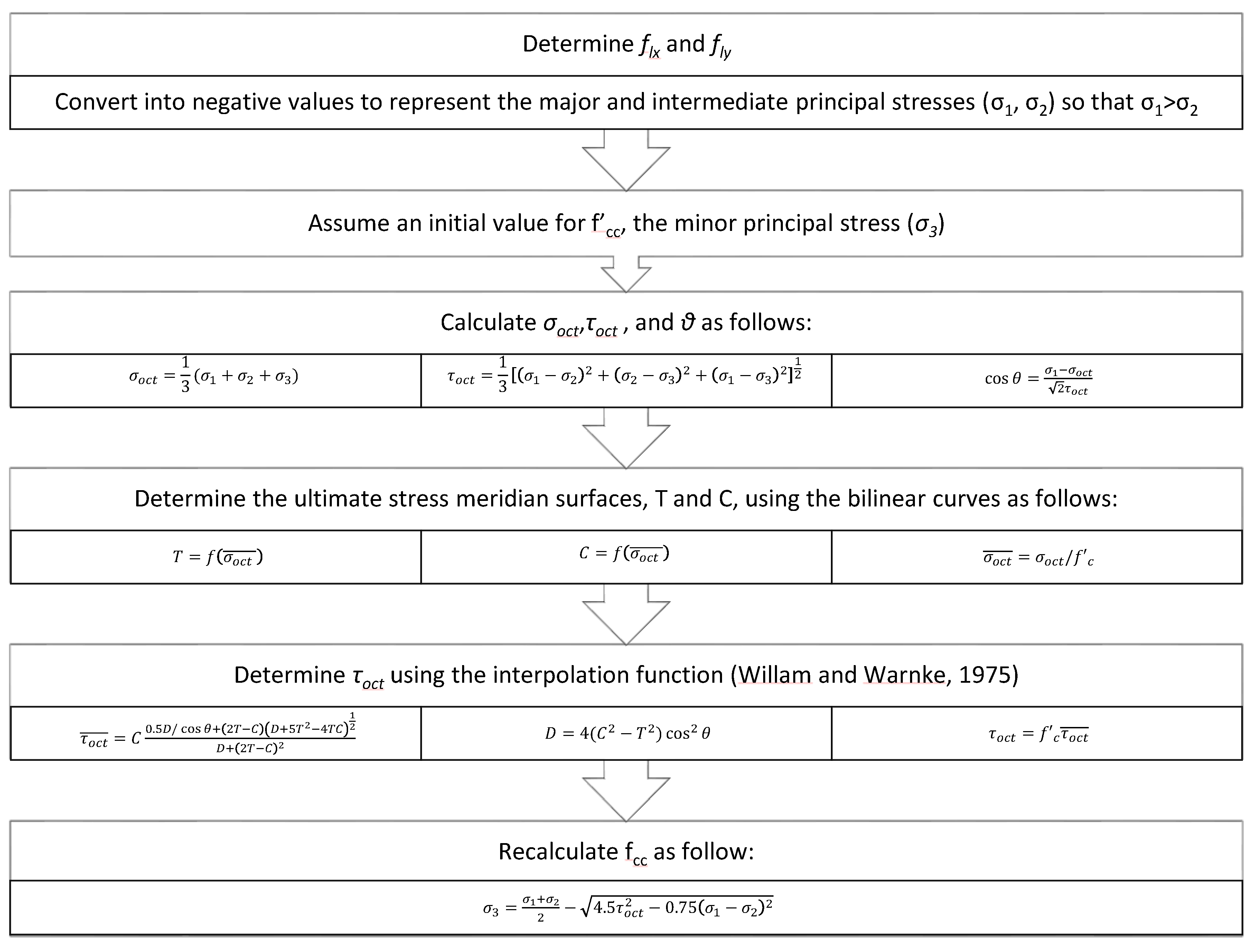
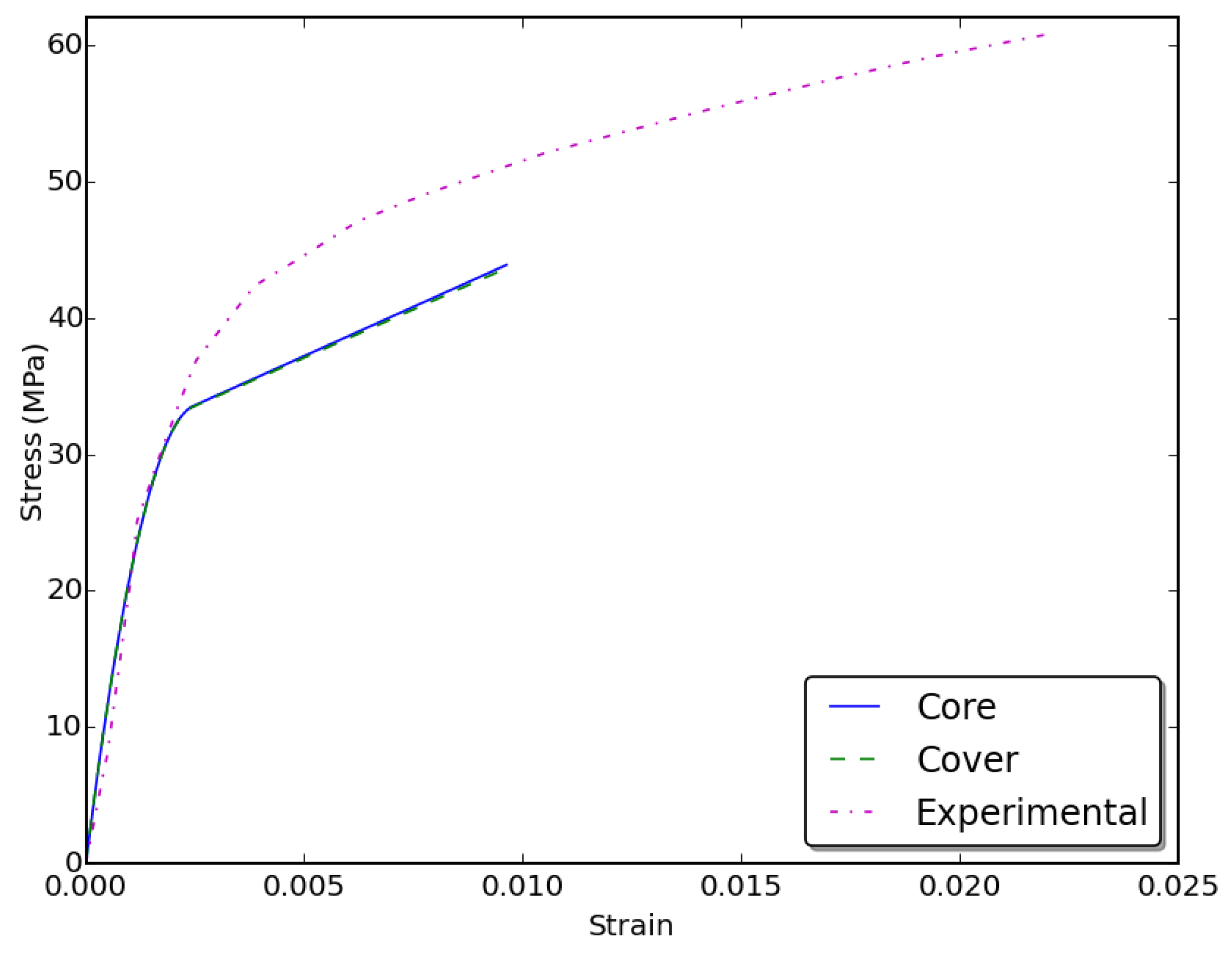
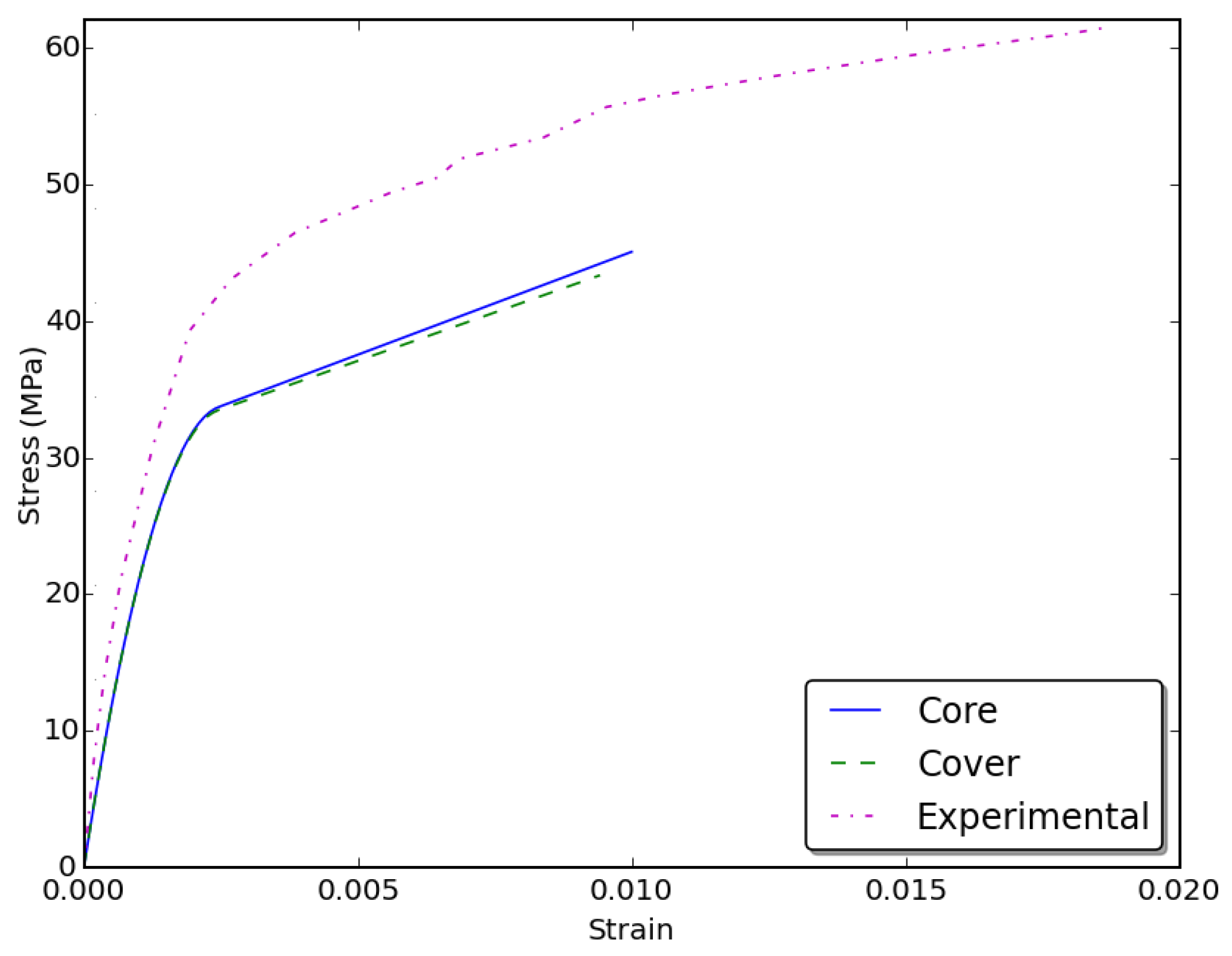
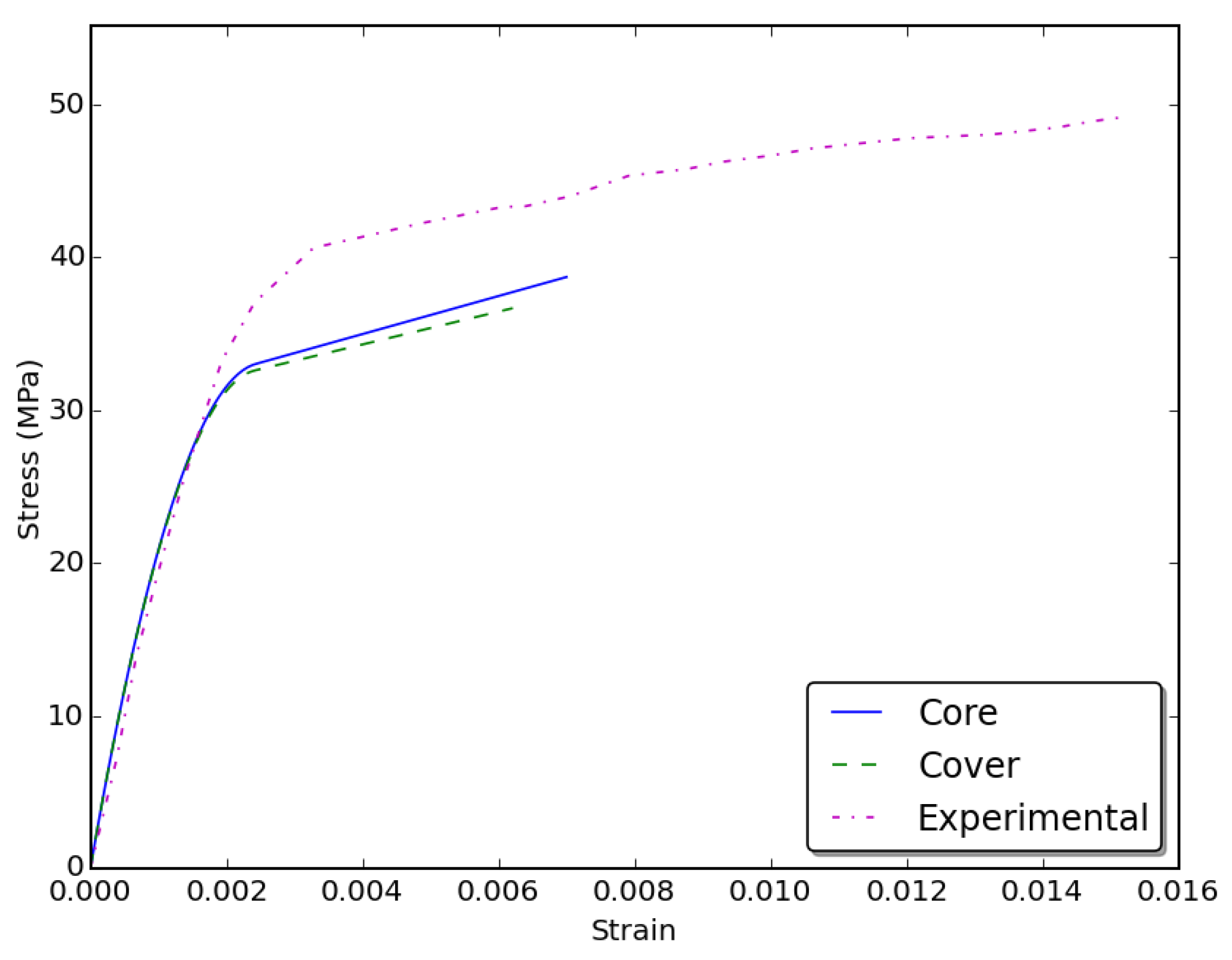
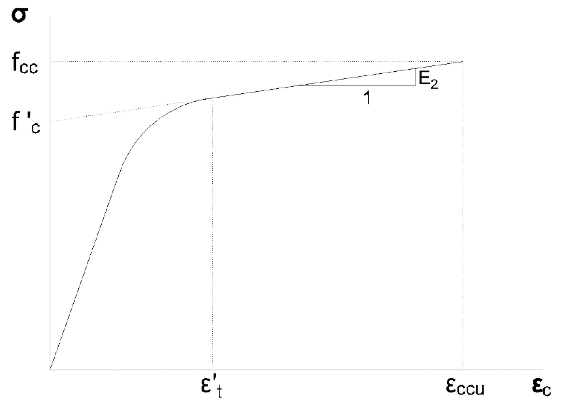
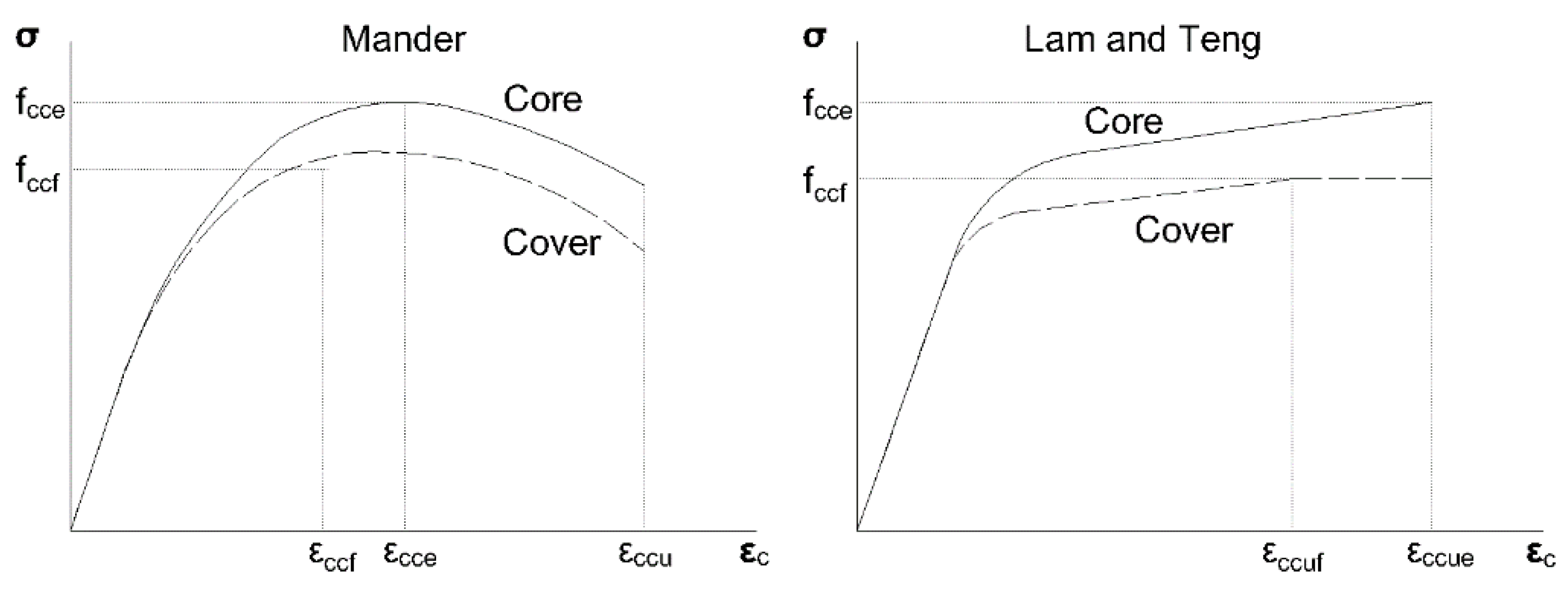
Overall, Figure 14, Figure 15, Figure 16 and Figure 17 indicate that the model provided reasonable results. For all four specimens, the slope of the first branch matched that of the experiment well. The slope of the second branch obtained from the model is close to that obtained from experimental data. However, the present model provided conservative results for the second branch of the stress-strain curve based on Lam and Teng’s equation calibration. It might also be observed that for these four cases, the cover and core stress-strain curves were very close. This is not always the case, as the curves vary depending on the specimen’s properties. To illustrate that, two samples with a 254 × 508 mm cross-section were analyzed. The section had a clear cover of 25.4 mm. Longitudinal reinforcement consisted of four bars in the x direction and five bars in the y direction of Size #8. Transverse reinforcement was provided by #3 rectilinear bars. Concrete compressive strength was taken to be 27.58 MPa, while the yield stress of longitudinal and transverse steel was 413.69 MPa. Tie spacing was taken to be 50.8 mm and 25.4 mm for the first and second samples, respectively. The stress-strain curves were obtained using the proposed model for both the core and the cover for Samples 1 and 2, as shown in Figure 18 and Figure 19, respectively.

Figure 14. Stress-strain curves for Specimen C30S100N4.

Figure 14. Stress-strain curves for Specimen C30S100N4.

Figure 15. Stress-strain curves for specimen C30S50N4.

Figure 15. Stress-strain curves for specimen C30S50N4.

Figure 16. Stress-strain curves for Specimen C30S100N2.

Figure 16. Stress-strain curves for Specimen C30S100N2.

Figure 17. Stress-strain curves for Specimen C30S50N2.

Figure 17. Stress-strain curves for Specimen C30S50N2.

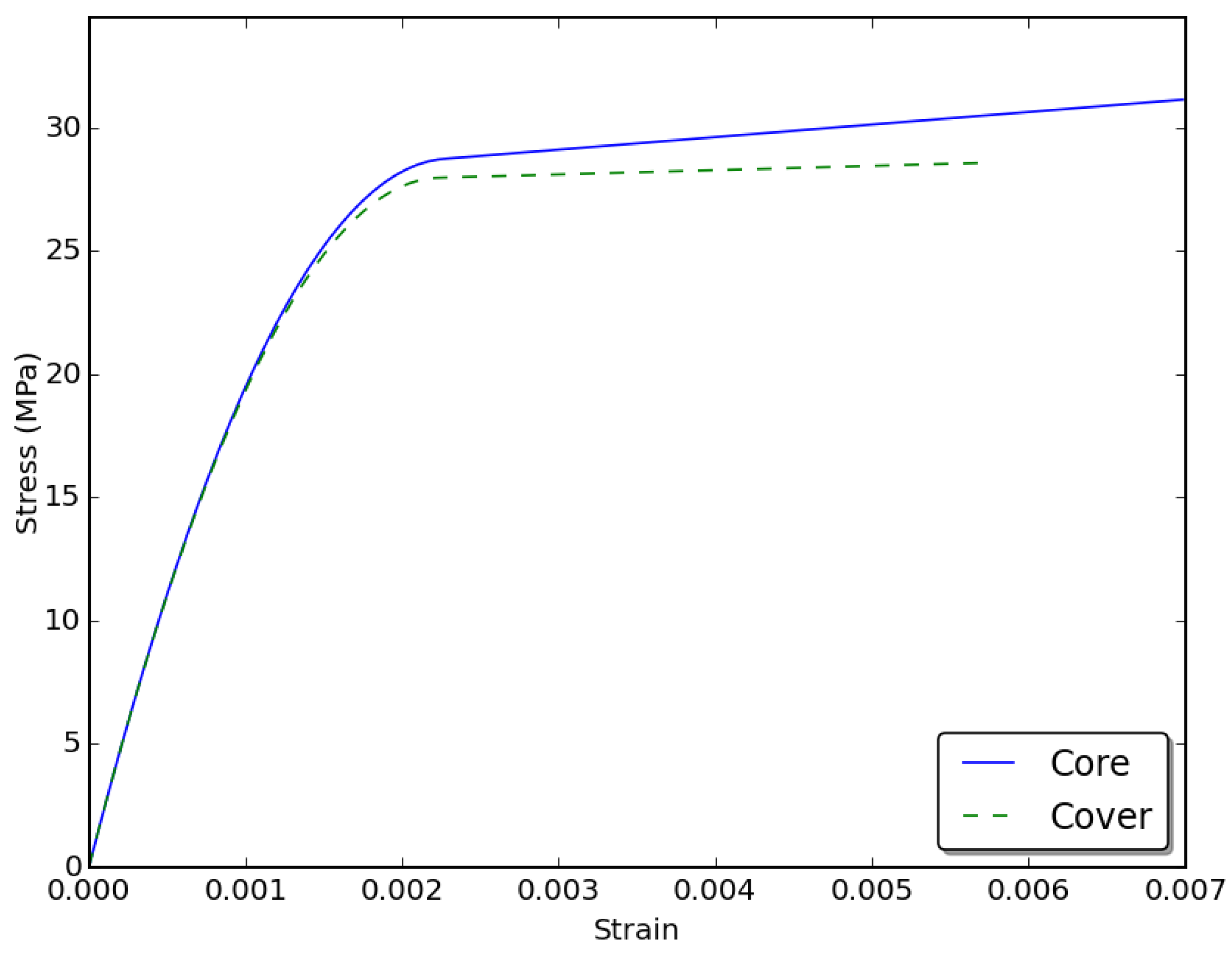
Figure 18. Stress-strain curve for Sample 1, s = 50.8 mm.

Figure 18. Stress-strain curve for Sample 1, s = 50.8 mm.

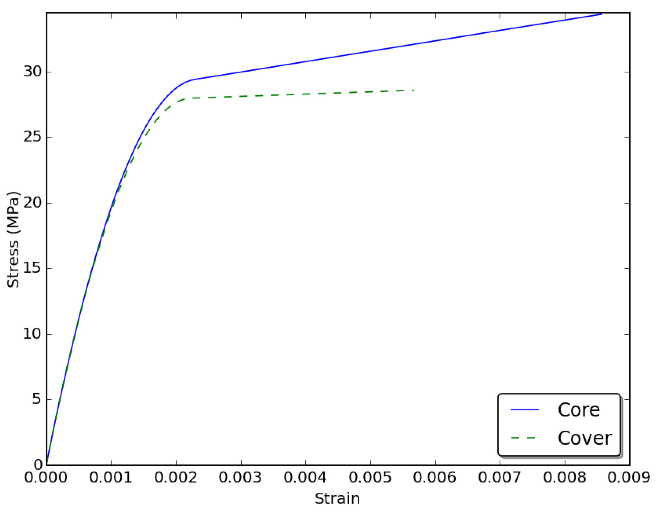
Figure 19. Stress-strain curve for Sample 1, s = 25.4 mm.

Figure 19. Stress-strain curve for Sample 1, s = 25.4 mm.

From Figure 18 and Figure 19, a considerable difference between the core and cover curves is observed. The difference is more significant when the transverse reinforcement is spaced closely. These two cases justify the independent consideration for the cover and core behaviors by the proposed model.

Wang and Hsu [26] investigated the axial load strength of rectangular and square reinforced compression members confined with GFRP jackets and steel ties. A total of six columns were prepared for testing (set 2). Three columns had a square section of 300 × 300 mm, and the remaining three had a rectangular section of 300 × 450 mm. Square sections had four 20-mm diameter Grade 430 steel bars with a bar at each corner. The bars were supported by rectilinear ties made of 10-mm diameter Grade 300 steel bars. The rectangular section had six 20-mm Grade 430 steel bars distributed uniformly. Rectilinear ties, made of 10-mm diameter Grade 300 steel bars, supported bars at the corners and connected the two bars at the midsection. Common properties are provided in Table 7. For each section type, there was an unconfined specimen (no FRP wraps), a section with two layers of FRP and a section with six layers of FRP. Properties for the steel reinforcement are provided in Table 8. Properties for the FRP jackets are provided in Table 9. Section-specific properties are provided in Table 10. All notations used are defined in Table 11.

Table 7. Common properties for set 2 specimens.

f′c	dl	Al	dt	At	rc	cc	s′
(MPa)	(mm)	(mm2)	(mm)	(mm2)	(mm)	(mm)	(mm)
19.03	20.07	314.19	9.91	78.71	29.97	29.97	180.09

Table 7. Common properties for set 2 specimens.

f′c	dl	Al	dt	At	rc	cc	s′
(MPa)	(mm)	(mm2)	(mm)	(mm2)	(mm)	(mm)	(mm)
19.03	20.07	314.19	9.91	78.71	29.97	29.97	180.09

Table 8. Steel properties for set 2 specimens.

Rebar Type	Es (GPa)	fy (MPa)	εu (%)
Longitudinal	200	439	6.67
Transverse	203	365	19

Table 8. Steel properties for set 2 specimens.

Rebar Type	Es (GPa)	fy (MPa)	εu (%)
Longitudinal	200	439	6.67
Transverse	203	365	19

Table 9. FRP properties for set 2 specimens.

Fiber Type	tf (mm)	Ef (GPa)	εf (%)	ffu (MPa)
GFRP	1.27	20.5	2	375

Table 9. FRP properties for set 2 specimens.

Fiber Type	tf (mm)	Ef (GPa)	εf (%)	ffu (MPa)
GFRP	1.27	20.5	2	375

Table 10. Section properties for set 2 specimens.

Code	b	h	Bars in x	Bars in y	n	flf/f′c	Pmax
	(mm)	(mm)			ply		(kN)
CS0	300	300	2	2	0	-	2128.83
CS2	300	300	2	2	2	0.151	2527.17
CS6	300	300	2	2	6	0.454	4028.44
CR0	300	450	2	3	0	-	3270.78
CR2	300	450	2	3	2	0.119	3601.06
CR6	300	450	2	3	6	0.356	4497.82

Table 10. Section properties for set 2 specimens.

Code	b	h	Bars in x	Bars in y	n	flf/f′c	Pmax
	(mm)	(mm)			ply		(kN)
CS0	300	300	2	2	0	-	2128.83
CS2	300	300	2	2	2	0.151	2527.17
CS6	300	300	2	2	6	0.454	4028.44
CR0	300	450	2	3	0	-	3270.78
CR2	300	450	2	3	2	0.119	3601.06
CR6	300	450	2	3	6	0.356	4497.82

Table 11. Notations for specifications.

Symbol	Description	Symbol	Description
b	Section width	fy	Longitudinal steel yield stress
h	Section height	f′c	Concrete compressive strength
cc	Clear cover	fyt	Transverse steel yield stress
rc	Radius of rounded corners	El	Longitudinal steel modulus of elasticity
Ef	FRP modulus of elasticity	Et	Transverse steel modulus of elasticity
εfu	FRP rupture strain	dl	Longitudinal bar diameter
tf	FRP ply thickness	Al	Longitudinal bar area
n	Number of FRP plies	dt	Transverse bar diameter
flf/f′c	Confinement ratio	At	Transverse bar area
Pmax	Maximum applied axial load	s′	Clear tie spacing

Table 11. Notations for specifications.

Symbol	Description	Symbol	Description
b	Section width	fy	Longitudinal steel yield stress
h	Section height	f′c	Concrete compressive strength
cc	Clear cover	fyt	Transverse steel yield stress
rc	Radius of rounded corners	El	Longitudinal steel modulus of elasticity
Ef	FRP modulus of elasticity	Et	Transverse steel modulus of elasticity
εfu	FRP rupture strain	dl	Longitudinal bar diameter
tf	FRP ply thickness	Al	Longitudinal bar area
n	Number of FRP plies	dt	Transverse bar diameter
flf/f′c	Confinement ratio	At	Transverse bar area
Pmax	Maximum applied axial load	s′	Clear tie spacing

The analysis on these specimens was performed using “KDOT Column Expert” confined columns analysis software, in which the proposed model was implemented. The axial capacity of each specimen was obtained and compared to the experimental results, as shown in Figure 18 and Figure 19.

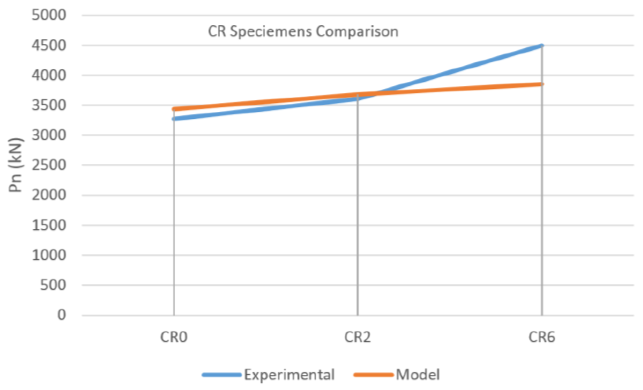
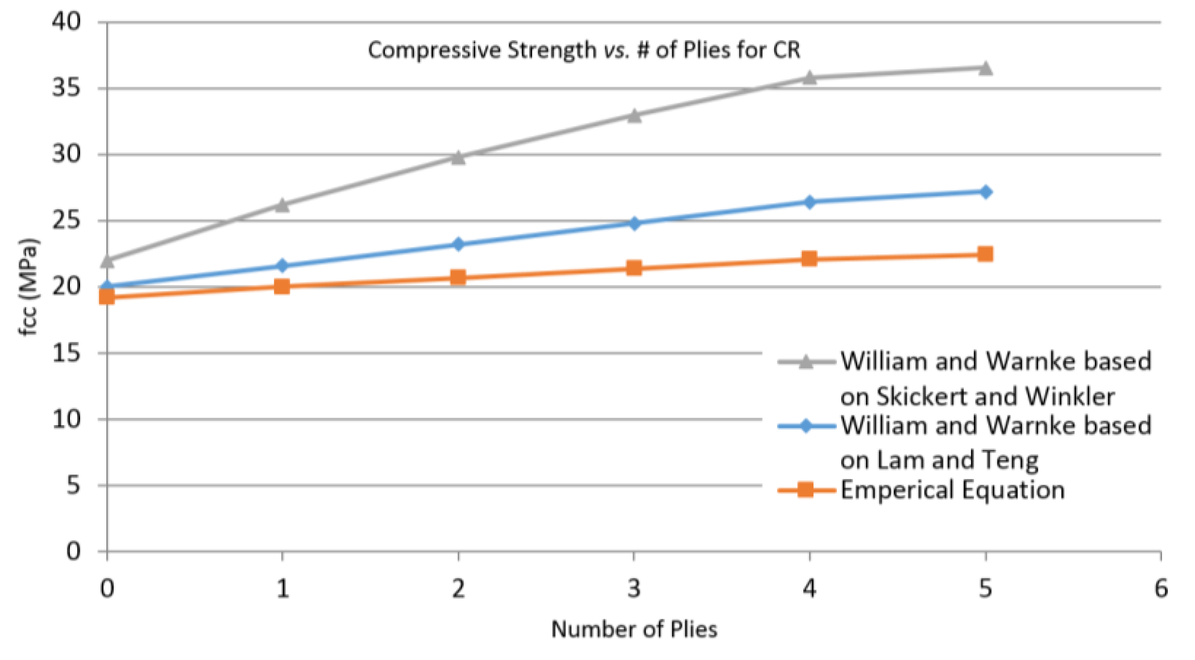
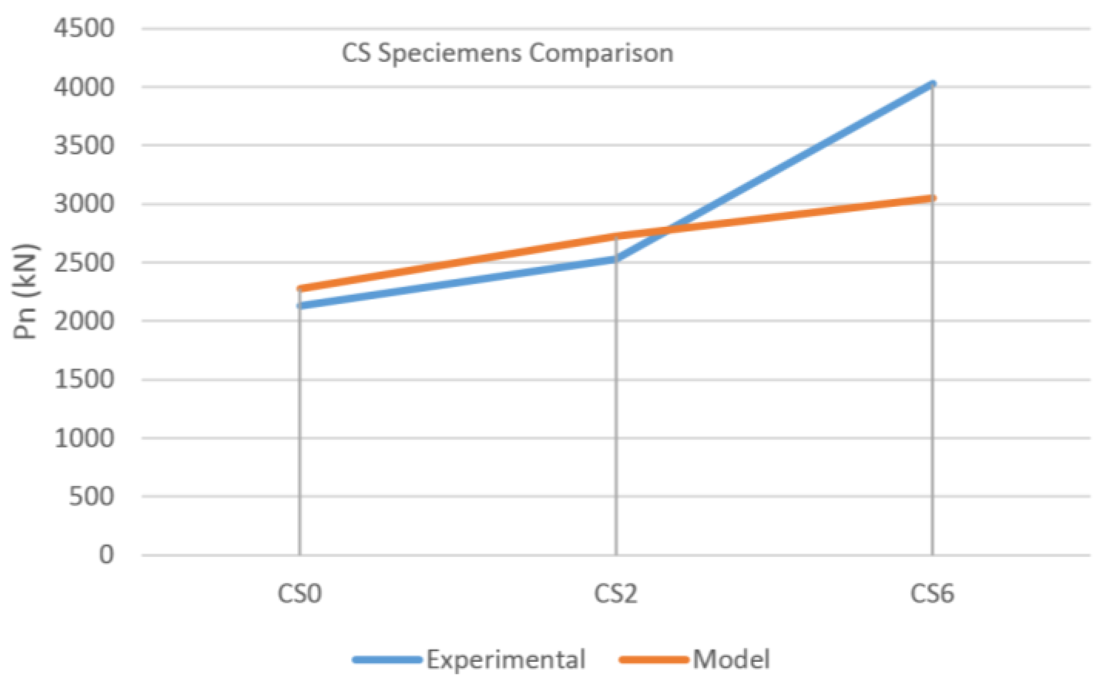
Figure 20 and Figure 21 show that the results obtained for unwrapped specimens and specimens with two wraps were very close to the results obtained for experiments. For specimens with six plies, the model provided conservative estimates for the axial capacity. As the main objective of developing this model was for extreme loading events analysis, obtaining somewhat conservative results is of most importance, as no reduction factors will be implemented in the extreme event analysis. It is observed that as expected, the axial capacity increased as the number of plies increased. The rate of the increase in the axial capacity using the model was lower than that obtained from experiments. Overall, the model provided reasonable results for the axial capacity for these specimens.

Figure 20. Analytic vs. experimental axial capacity comparisons for square specimens.

Figure 20. Analytic vs. experimental axial capacity comparisons for square specimens.

Figure 21. Analytic vs. experimental capacity comparisons for rectangular specimens.

Figure 21. Analytic vs. experimental capacity comparisons for rectangular specimens.

6.2. Parametric Study

In order to validate the proposed approach and observe the behavior of the combined model and the programmed algorithm, a parametric study was conducted. The common properties are provided in Table 12. They include the compressive strength (f’_c), clear cover (cc), radius of rounded corners (r_c), ties bar size and their clear spacing (s’), yield strength (f_y) and modulus of elasticity (E_s) for both longitudinal and lateral reinforcement and FRP properties, such as modulus of elasticity (E_f), rupture strain (ε_fu) and ply thickness (t_f).

Table 12. Common properties for the parametric study.

Property	f′c (MPa)	cc (mm)	rc (mm)	Tie Size	s’ (mm)	fy (MPa)	Es (MPa)	Ef (MPa)	εfu	tf (mm)
Value	27.58	25.4	25.4	#3	38.1	413.69	199948	229940	0.015	0.127

Table 12. Common properties for the parametric study.

Property	f′c (MPa)	cc (mm)	rc (mm)	Tie Size	s’ (mm)	fy (MPa)	Es (MPa)	Ef (MPa)	εfu	tf (mm)
Value	27.58	25.4	25.4	#3	38.1	413.69	199948	229940	0.015	0.127

The properties for the longitudinal reinforcement, which was one of the variables, are provided in Table 13. This table provides the sections’ dimensions, their bar sizes, their count along the x and y-axes and the steel ratio (ρ).

Table 13. Section geometry and longitudinal reinforcement details.

Section (mm)	Bar Size	Bars in x	Bars in y	ρ
305 × 305	#5	4	4	0.0258
305 × 610	#4	4	5	0.0292
305 × 915	#8	4	6	0.0293
305 × 1220	#8	4	8	0.0312

Table 13. Section geometry and longitudinal reinforcement details.

Section (mm)	Bar Size	Bars in x	Bars in y	ρ
305 × 305	#5	4	4	0.0258
305 × 610	#4	4	5	0.0292
305 × 915	#8	4	6	0.0293
305 × 1220	#8	4	8	0.0312

All sections listed above were analyzed while varying the number of FRP layers from zero to four. The proposed model was then used to obtain the axial capacity (P_n) for each section. These values are provided in Table 14. The percentage difference (PD) is also shown and was calculated between the specific number of wraps in question and the unwrapped specimen’s capacity.

At the first glance, it appears from the data shown in Table 14 that adding more FRP layers to some cases (shaded in gray in the table) does not increase the axial capacity of the section. In order to investigate, compressive strength values for both the core (f_cce) and the cover (f_ccf) were computed for two sample cases of 305 × 610 mm and 305 × 1220 mm sections. Extracted parameters are listed in Table 15.

Table 14. Parametric study results. PD, percentage difference.

Section, mm	n	Pn, kN	PD	Section, mm	n	Pn, kN	PD
305 × 305	0	4147.39	-	305 × 915	0	11,771.24	-
	1	4389.51	0.06		1	11,834.58	0.01
	2	4571.08	0.10		2	11,897.93	0.01
	3	4671.97	0.13		3	11,897.93	0.01
	4	4732.46	0.14		4	11,961.31	0.02
305 × 610	0	8135.26	-	305 × 1220	0	15,644.44	-
	1	8261.82	0.02		1	15,726.91	0.01
	2	8346.20	0.03		2	15,726.91	0.01
	3	8388.37	0.03		3	15,726.91	0.01
	4	8388.37	0.03		4	15,726.91	0.01

Table 14. Parametric study results. PD, percentage difference.

Section, mm	n	Pn, kN	PD	Section, mm	n	Pn, kN	PD
305 × 305	0	4147.39	-	305 × 915	0	11,771.24	-
	1	4389.51	0.06		1	11,834.58	0.01
	2	4571.08	0.10		2	11,897.93	0.01
	3	4671.97	0.13		3	11,897.93	0.01
	4	4732.46	0.14		4	11,961.31	0.02
305 × 610	0	8135.26	-	305 × 1220	0	15,644.44	-
	1	8261.82	0.02		1	15,726.91	0.01
	2	8346.20	0.03		2	15,726.91	0.01
	3	8388.37	0.03		3	15,726.91	0.01
	4	8388.37	0.03		4	15,726.91	0.01

Table 15. Extracted analysis parameters.

Section	305 × 610 mm		305 × 1220 mm
nf	3	4	1	2	3	4
flf/f′c	0.082	0.109	0.015	0.03	0.044	0.059
fcce (MPa)	35.78	35.58	32.06	32.11	32.16	32.13
fccf (MPa)	28.48	28.75	27.64	27.7	27.76	27.81

Table 15. Extracted analysis parameters.

Section	305 × 610 mm		305 × 1220 mm
nf	3	4	1	2	3	4
flf/f′c	0.082	0.109	0.015	0.03	0.044	0.059
fcce (MPa)	35.78	35.58	32.06	32.11	32.16	32.13
fccf (MPa)	28.48	28.75	27.64	27.7	27.76	27.81

Before proceeding, it is observed that the confined compressive strength has dropped for the first case from 35.78 MPa to 35.58 MPa and for the second case from 32.16 MPa to 32.13 MPa as the number of FRP layers is increased from 3–4 layers in each case. This occurred even though the confining pressure has increased since the number of FRP layers increased. The cause of this issue is the restriction on the ultimate strain imposed by ACI440.2R-08 [8]. In these two instances, the strain obtained exceeded 0.01, and thus, a new f_cc value corresponding to this ultimate strain is calculated.

For the first case, as the confinement ratio (f_lf/f′_c) is greater than 0.08, the model used is the Lam and Teng model with an ascending second branch. Detailed calculations will be provided to verify the results obtained from the program for this case. The areas are calculated as follows:

$$b_c=b-2cc-d_t=305-50.8-9.53=244.67 \text{mm}$$

$$h_c=h-2cc-d_t=610-50.8-9.53=549.67 \text{mm}$$

$$A_{core}=b_c·h_c-n·A_s=134,488-14\times 387.1=129,068.4{ \text{mm}}^2$$

$$A_{cover}=b·h-b_c·h_c=186,050-134488=51,562{ \text{mm}}^2$$

$\text{where} b_c=\text{confined core width};$ $h_c=\text{confined core depth};$ $cc=\text{clear cover};$ $d_t=\text{tie diameter};$ n = number of longitudinal bars; $A_s=\text{longitudenal bar area};$ $f_y=$yield stress for longitudinal reinforcement.

Using the extracted value from Table 15 and the calculated areas, the axial capacity is calculated as follows:

$$P_n=f_{cce}·A_{core}+f_{ccf}·A_{cover}+f_y·n·A_s$$

P₃ = 35.78 × 129068.4 + 28.48 × 51562 + 414 × 14 × 387.1 = 8330.2 × 10³ N

$$P_4=35.58\times 129068.4+28.75\times 51562+414\times 14\times 387.1=8318.3 \times {10}^3 N$$

$\text{where} P_3=\text{axial capacity of specimen with three layers}$; $P_4=$axial capacity of specimen with four layers.

As can be seen from the calculation, the capacity has actually dropped when the number of FRP layers was increased. The values are very close (the percentage difference is 0.14%) and are smaller than the step size used by the incremental solver, which caused the program to provide the same results for both sections. Similarly, for the second case, the change in confined strength values is very small due to the high aspect ratio. In this case, the Mander model is used, since the confinement ratio is below 0.08. The small change in confined strength is not significant enough for the solver and results in an axial capacity difference that is smaller than the step size. This again causes the program to output the same axial capacity for all sections under this case. Calculation details for the second case are shown below:

$$b_c=b-2cc-d_t=305-50.8-9.53=244.67 \text{mm}$$

$$h_c=h-2cc-d_t=1220-50.8-9.53=1159.67 \text{mm}$$

$$A_{core}=b_c·h_c-n·A_s=283,736.5-20\times 509.7=273,543 {\text{mm}}^2$$

$$A_{cover}=b·h-b_c·h_c=372,100-283,736.5=88,363.5 {\text{mm}}^2$$

$$P_3=32.16\times 273,543+27.76\times 88,363.5+414\times 20\times 509.7=15,470.4 \times {10}^3 \text{N}$$

$$P_4=32.13\times 273,543+27.81\times 88,363.5+414\times 20\times 509.7=15,466.64 \times {10}^3 \text{N}$$

Overall, the results shown in Table 14 were reasonable. Generally, the axial capacity has mostly increased as the number of FRP layers increased. It is observed that the increase in axial capacity due to the addition of FRP is diminished in sections with higher aspect ratios. This is expected because the FRP confinement effect is highly dependent on the aspect ratio. It is concluded that the proposed model functions properly and provides reasonable results.

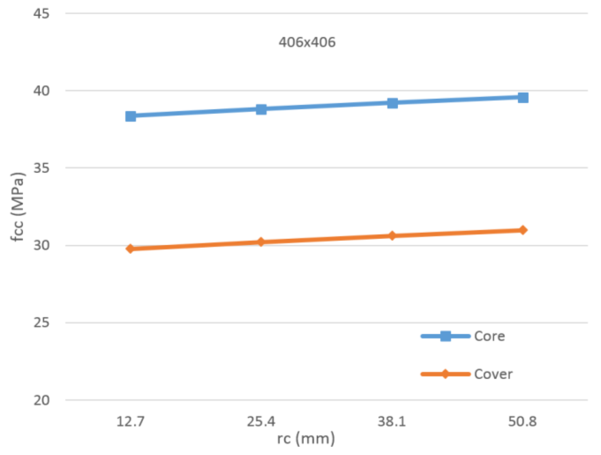
Additionally, another parametric study was conducted to evaluate the effect of the radius of rounded corners (r_c) parameter on the axial capacity. Two sections were chosen for this analysis, namely 406 × 406 mm and 406 × 812 mm. The number of FRP plies was fixed at two CFRP plies. The evaluated radius of rounded corners values were 12.7 mm, 25.4 mm, 38.1 mm and 50.8 mm. The minimum radius of rounded corner was taken to be 12.7 mm as per the provisions of ACI440.08-2R [8]. For each of the sections analyzed, the confined compressive strength was obtained for both the core and the cover, as shown in Figure 22 and Figure 23.

Figure 22. Core and cover confined strengths for the section of 406 × 406 mm.

Figure 22. Core and cover confined strengths for the section of 406 × 406 mm.

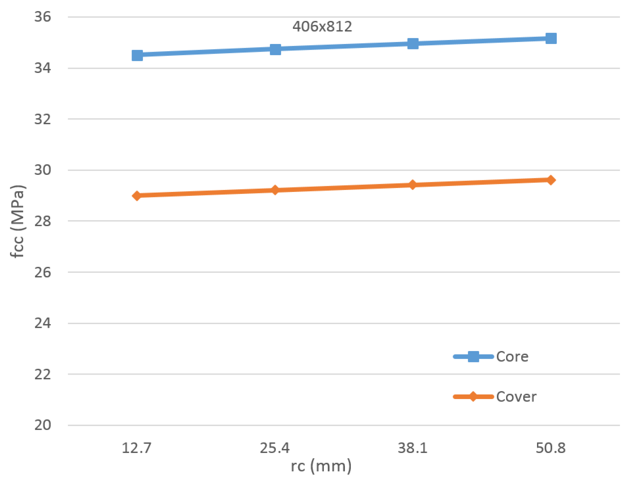
Figure 23. Core and cover confined strengths for the section of 406 × 812 mm.

Figure 23. Core and cover confined strengths for the section of 406 × 812 mm.

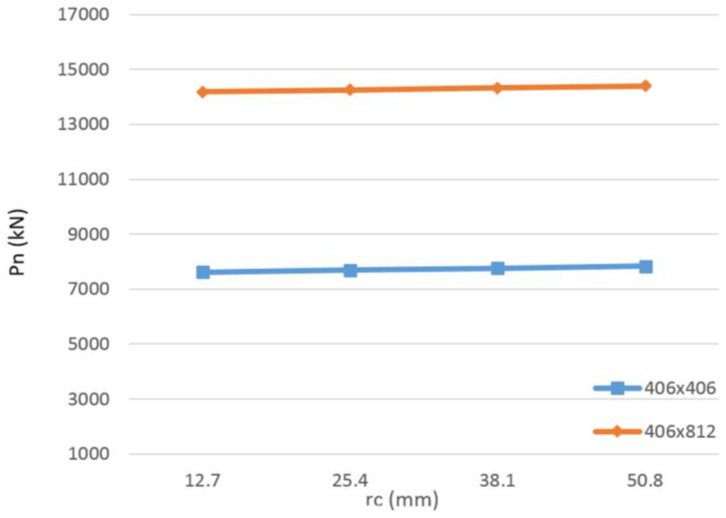
As expected, the confined strength increased as the radius of rounded corners increased. The trend was observed to be closely linear (R² = 99%). A considerable difference between the core and the cover strengths was also observed. The increase in the confined strength for the cover from the least to highest radius of rounded corner was obtained to be 4.04% and 2.12% for the square and rectangular sections, respectively. In addition to the confined strength values, the axial capacity of the section (P_n) was also obtained, as shown in Figure 24. The behavior observed was similar to that of the confined strength. For the square section, each increase of 12.7 mm in the radius of rounded corners resulted in an increase of approximately 1% in the axial capacity. This increase was obtained to be approximately 0.5% in the rectangular section. Overall, the increase in the radius of rounded corners provided a small increase in the confined strength and, thus, the axial capacity of the sections.

Figure 24. Axial capacity variation for sections of 406 × 406 mm and 406 × 812 mm.

Figure 24. Axial capacity variation for sections of 406 × 406 mm and 406 × 812 mm.

Additionally, in order to demonstrate the effect of the confinement parameters, a 406 × 406 mm specimen with the properties provided in Table 12 was analyzed. The ultimate capacity of the section was obtained for the unconfined case, steel confinement only (Mander [4]), FRP confinement only (Lam and Teng [6]) and combined confinement (present model). The capacities were obtained to be 3703 kN, 3981 kN, 4365 kN and 4835 kN, respectively. The proposed model provided increases in the ultimate capacity of approximately 21% and 11% from the individual steel and FRP cases, respectively. It should be noted that the combined effect of the confinement depends on the parameters of the individual confinement systems, that is the steel and FRP, and improvement in the ultimate capacity will vary based on these parameters.

7. Conclusions

In this study, a model was proposed to combine FRP and steel confinement in rectangular reinforced concrete columns. From previously-conducted research, the Mander model [4] was found to be the most suitable confinement model for transverse steel. Based on the conducted literature review and the recommendations of the special report by the ACI Committee 440 task group on FRP confinement [7], the Lam and Teng [6] model was found to be the most suitable confinement model for FRP. A triaxial constitutive model for confined concrete was calibrated and implemented in the proposed combined model. The proposed model was then used to obtain stress-strain curves and the axial capacities for experimental cases found in the literature. The proposed model results showed good agreement with the experimental data. Additionally, the results were shown to be conservative for most of the tested cases. Furthermore, a parametric study was conducted after validating the proposed model. The objective of the parametric study was to examine the behavior of the model for cases beyond what was validated with experiments and ensure its consistency. The model provided reasonable results, and its consistency was validated based on them. It is concluded that the combined confinement model is a viable tool to accurately model confinement in rectangular concrete columns with both transverse steel and FRP.