Article

Electrochemical Impedance Spectroscopy and Equivalent Circuit Modeling of Low-Impedance Lithium-Ion Battery Cells for Electric Vehicles

1
Department of Mechanical Engineering, George Mason University, Fairfax, VA 22030, USA
2
Reliability Engineering Services, Ansys Part of Synopsys, Beltsville, MD 20705, USA
3
Center for Collision Safety and Analysis, George Mason University, Manassas, VA 20110, USA
*
Author to whom correspondence should be addressed.
These authors contributed equally to the work.
Coatings 2026, 16(8), 930; https://doi.org/10.3390/coatings16080930
Submission received: 8 April 2026 / Revised: 20 June 2026 / Accepted: 22 July 2026 / Published: 4 August 2026

Abstract

Accurate electrochemical impedance spectroscopy (EIS) characterization of low-impedance (<1 mΩ) lithium-ion battery cells used in electric vehicles is challenging because resistance and inductance in the measurement pathway can be comparable to the intrinsic cell impedance. This study investigates an EV-grade, large-format commercial lithium-ion pouch cell using a four-terminal EIS configuration and a custom connection fixture designed to maintain low and consistent contact resistance and reduce measurement-pathway effects. The EIS measurements shows good repeatability, and their linearity was confirmed using the Kramers–Kronig validity test. Impedance spectra acquired under selected state-of-charge (SOC) and temperature conditions were interpreted using an equivalent circuit model comprising an effective series inductance, an ohmic resistance, a constant phase element, a charge-transfer resistance, and a generalized Warburg element. Bayesian optimization followed by Nelder–Mead refinement was applied for parameter identification. The selected model represents the measured inductive, interfacial, and diffusion-related features as effective lumped responses rather than as a unique mechanistic decomposition. Across the SOC conditions investigated, the fitted ohmic resistance and charge-transfer resistance generally decreased as the temperature increased from 25 °C to 40 °C. By reducing the measurement errors related to the connection method rather than relying solely on instrument-side accuracy improvements, this work provides a practical approach for EIS measurements of milliohm-scale battery cells. These results establish a foundation for future temperature-compensated impedance diagnostics and further investigation of interfacial and transport behavior in EV battery cells.

1. Introduction

Lithium-ion batteries (LIBs) have been widely adopted in electric vehicles (EVs) due to their high energy density and prolonged cycle life [1,2]. The safe operation of lithium-ion batteries requires a battery management system (BMS), an electronic control system designed to maintain the battery within its optimal operating conditions and prevent critical issues such as overcharging, over-discharging, and thermal runaway [3,4]. Conventional BMS in EVs primarily rely on measurements of cell voltage, current, and temperature to estimate the battery’s state of charge (SOC) and state of health (SOH). This approach provides limited accuracy due to its lack of direct insight into the electrochemical processes within the battery cells [5]. In recent years, the integration of EIS into onboard BMS has shown significant potential [6,7,8,9] for addressing these limitations.
EIS is a non-destructive testing technique that provides detailed insights into the internal electrochemical processes within battery cells. By applying a small-amplitude AC voltage (or current) signal across a range of frequencies and measuring the resulting current (or voltage) response, the battery’s impedance characteristics can be accurately determined. The impedance spectrum reflects different electrochemical reactions at the electrode–electrolyte interface, including charge transfer, adsorption, desorption, diffusion, double-layer effect, solid electrolyte interface (SEI) growth, lithium plating, and other related phenomena [10,11]. EIS data can be used to estimate the state of charge (SOC) and state of health (SOH), characterize performance degradation, and predict potential battery failure [12,13,14]. An equivalent circuit model (ECM) is used to interpret the impedance spectrum, where each circuit component corresponds to a specific electrochemical process occurring within the battery [15,16]. EIS enables more accurate diagnosis of SOC and SOH, since it is directly related to the electrochemical processes [17].
The classical EIS technique typically employs a three-electrode system [18,19], which remains widely used for testing electrochemical kinetics in half-cell configurations and for measuring commercial battery cells with relatively high impedance (>10 mΩ) [20,21,22,23]. However, high-performance LIBs in EVs typically exhibit very low impedance in the range of 1–10 mΩ [17,24,25]. It has been reported that such low impedance can lead to reduced accuracy and repeatability issue in EIS measurements [26]. In such cases, a four-electrode system, also known as Kelvin sensing, offers higher accuracy and is recommended [27,28]. The four-electrode configuration uses two electrodes for current injection and two separate electrodes for voltage measurement, isolating the voltage measurement from current-carrying leads. This setup reduces the influence of test leads’ impedance on the measurement, as the voltage sensing electrode carries negligible current. Consequently, the measured voltage drop is attributed solely to the measured electrochemical system. This approach is necessary for accurately characterizing low-impedance cells.
The impedance of test leads and contact resistance are the major contributors to measurement error. For example, a 1 m long 14 American wire gauge (AWG) solid core copper wire has a resistance of approximately 8 mΩ, and the resistance of alligator clips is around 10 mΩ. Beyond the four-electrode method, the key point to further improve measurement accuracy is to reduce the resistance and inductance of the test leads. The following methods have been reported in the literature, including the use of coaxial [29] or low-resistance conductors [30], shortened or geometrically arranged leads [16], four-terminal sensing [31], reduced mutual inductance [32], and high-current excitation [33].
An equivalent circuit model is commonly used to interpret EIS results by providing an electrical circuit representation of the underlying electrochemical processes. The simplest steady-state equivalent circuit model of a battery consists of a voltage source in series with an internal resistor ( R i ). A lower internal resistance is desirable for high-performance cells, as it allows more electrical power to be delivered to the external circuit and generating less heat within the battery.
The theoretical foundation for EIS modeling is rooted in linear systems theory, developed by Oliver Heaviside in the 19th century. This framework enabled the representation of dynamic systems using linear differential equations and frequency-domain analysis. Later, Warburg extended the concept of impedance to electrochemical systems, introducing models for electrified interfaces and diffusion processes [29]. With the advancement of potentiostat and frequency response analyzers, EIS has been applied to a broad range of systems and phenomena, including ionic and electronic conduction heterogeneous reactions, and mass transport processes [30]. The impedance characteristics of common electrical components used in ECMs are summarized in Table 1. The Randles circuit is widely used to model the transient electrochemical behavior of a battery under non-steady-state conditions; the double-layer capacitance ( C d l ) is connected in parallel with a series combination of the charge-transfer resistance ( R c t ) and the Warburg impedance ( W ), and this parallel network is placed in series with the solution resistance ( R s ) [31]. Physically, R c t represents the charge-transfer processes at the electrode–electrolyte interface, C d l accounts for charge accumulation within the electrochemical double layer, and the Warburg element stands for the frequency-dependent diffusion of ions in the electrolyte.
The advanced equivalent circuit model introduces fractional-order elements, i.e., the constant phase element ( C P E ) and the generalized Warburg element ( W G ), in addition to the integer-order components, C d l , R c t , and R s . The C P E can be considered a non-ideal capacitor that accounts for surface energy distribution heterogeneity and non-ideal geometric features [32,33]. The classic Randles circuit is typically modified by replacing the ideal capacitor with a C P E . The impedance of C P E is shown in Table 1, where α is the C P E exponent and Q is the C P E parameter [34], j is the imaginary number unit, and ω is the angular frequency. When α = 1 , the C P E is an ideal capacitor. The Warburg element is used to characterize mass diffusion phenomena, and it varies depending on diffusion method and boundary conditions. Four types of Warburg elements are frequently used: ideal Warburg, finite-diffusion Warburg (finite-length), finite-space Warburg, and generalized diffusion Warburg. The ideal Warburg represents a semi-infinite linear diffusion and appears as a straight line with a slope of 45 ° in a Nyquist plot. In contrast, the finite Warburg impedance accounts for diffusion over a limited space or length, where the terminus of diffusion is not infinitely far from the electrode as in the ideal Warburg. Specifically, finite-length Warburg ( W s ) corresponds to a transmission boundary condition, while finite-space diffusion ( W o ) corresponds to a reflective boundary condition. A generalized Warburg element is applied in anomalous diffusion, where deviations from ideal behavior occur [35,36,37,38]. γ , used in the generalized Warburg element, represents the parameter of mesoporous electrode roughness; when γ is 1, the electrode is absolutely smooth [36,39,40]. The generalized Warburg element can be expressed as the equation in Table 1. T is the characteristic diffusion time(s), where T = L 2 / D , T is the diffusion length, and D is the diffusion coefficient. In the present lumped ECM implementation, however, T is treated as a model-dependent frequency-scaling parameter and is not assumed a priori to represent the solid-state lithium-ion diffusion time directly.
Table 1. Commonly used electric components in equivalent circuit model.
NameImpedanceRepresentation in Nyquist Citation
Solution resistance Z R s = R s Intersection of the real axis
Charge-transfer resistance Z R c t = R c t Diameter of semicircle
Double layer capacitor Z C d l = j ω C d l Vertical line goes up as frequency gets lower[31]
Solid-electrolyte interface resistance Z R s e i = R s e i Intersection of the small semicircle to the real axis
Solid-electrolyte interface capacitor Z C s e i = j ω C s e i Vertical line goes up as frequency gets lower[31]
Constant phase element Z C P E = 1 Q j ω α Line with slope (slope depending on α )[41]
Classic Warburg Z w = σ j ω 45° line in low-frequency region[29]
Finite-length Warburg Z W s = R w j T ω tanh j T ω Transition from 45° line to semicircle[42]
Finite-space Warburg Z W o = R w j T ω coth j T ω Transition from 45° line to vertical line[43]
Generalized Warburg Z W G = R w ( j T ω ) γ / 2 coth [ ( j T ω ) γ / 2 ] Line with angle between 0° and 90° depending on γ / 2 [43,44]
Inductance Z L = j ω L Move plot downward
After selecting an ECM model with physical meaning, accurate characterization of EIS modeling parameters is critical for correlating with experimental data. Several optimization algorithms have been reported for extracting ECM parameters from EIS results, including the Levenberg–Marquardt algorithm (LM) [45], differential evolution algorithm (DE) [46], random mutation differential evolution (RMDE) [47], particle swarm optimization (PSO) [48], simulate annealing (SA) [49], genetic algorithm (GA) [50] and Monté Carlo method [51]. However, these optimizations are not considered data-driven methods. As a data-driven approach, Bayesian optimization (BO) constructs a surrogate model based on a Gaussian process [52]. This sequential method leverages all historical data. The next sampling point is selected by balancing exploration and exploitation through an acquisition function. In this study, Bayesian optimization followed by Nelder–Mead refinement was applied to identify the parameters of the selected ECM for the measured low-impedance EV-cell spectra.
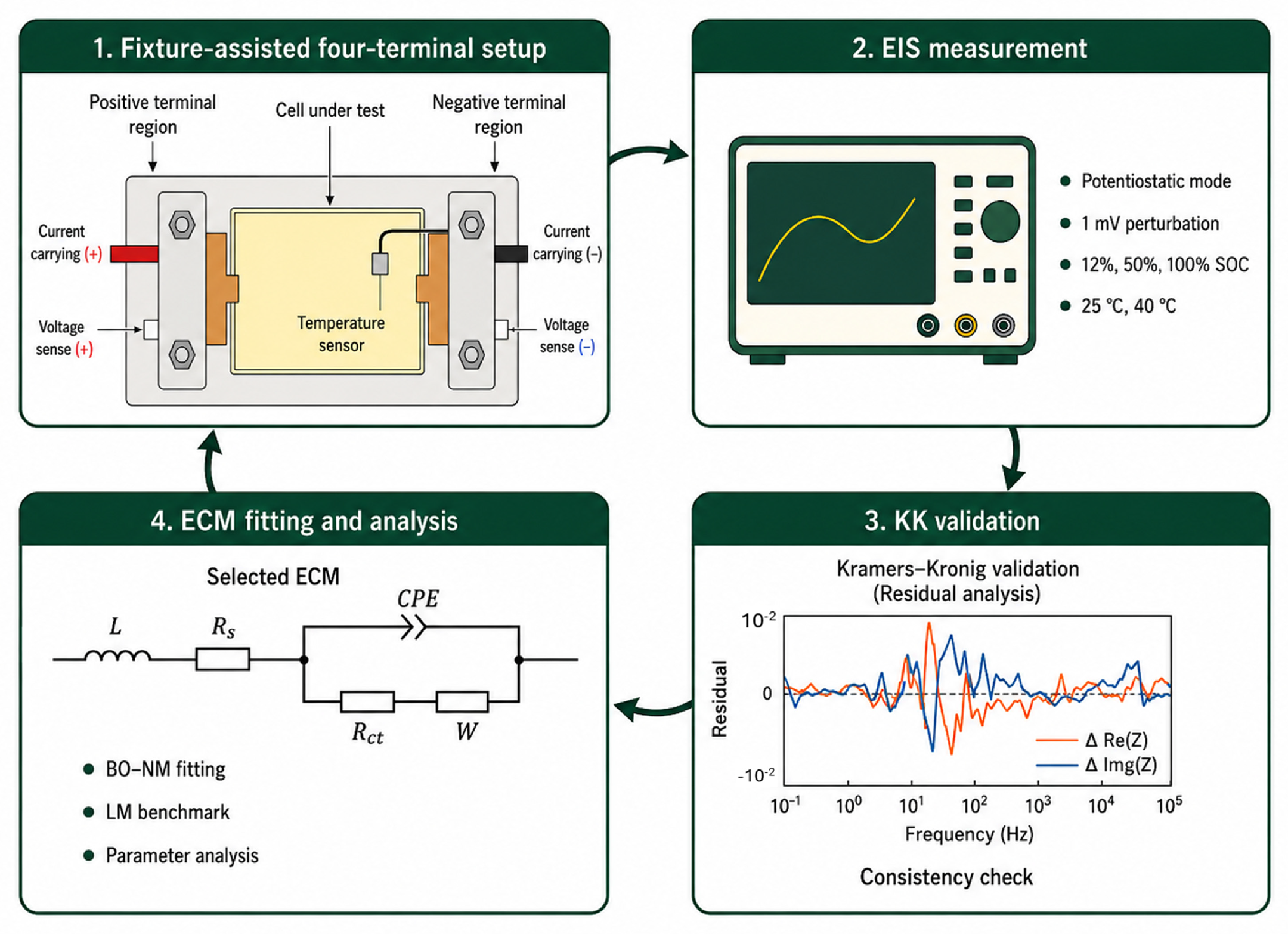
The primary objective of this work is to characterize commercial LIBs with impedance values around 1 mΩ. EIS measurements were performed on an EV cell placed inside a thermal chamber, under varying states of charge and temperatures, using an EIS analyzer together with a battery cycler. A customized connection fixture was employed to connect the test leads to the battery cell. The Bode and Nyquist plots were generated with an excitation signal of 1 mV. An equivalent circuit model was developed to interpret the EIS results, including the solution resistance R s , charge transfer resistance R c t , constant phase element C P E and generalized Warburg diffusion element W G . Bayesian optimization was used for ECM parameter characterization. This data-driven optimization framework is proposed as an effective method for identifying ECM parameters for EV battery characterization. Our results provide a comprehensive view of the impedance spectrum and ECM characterization for a high-performance commercial lithium-ion battery cell. The work is illustrated in Figure 1.

2. Methodology

2.1. EIS Test Setup

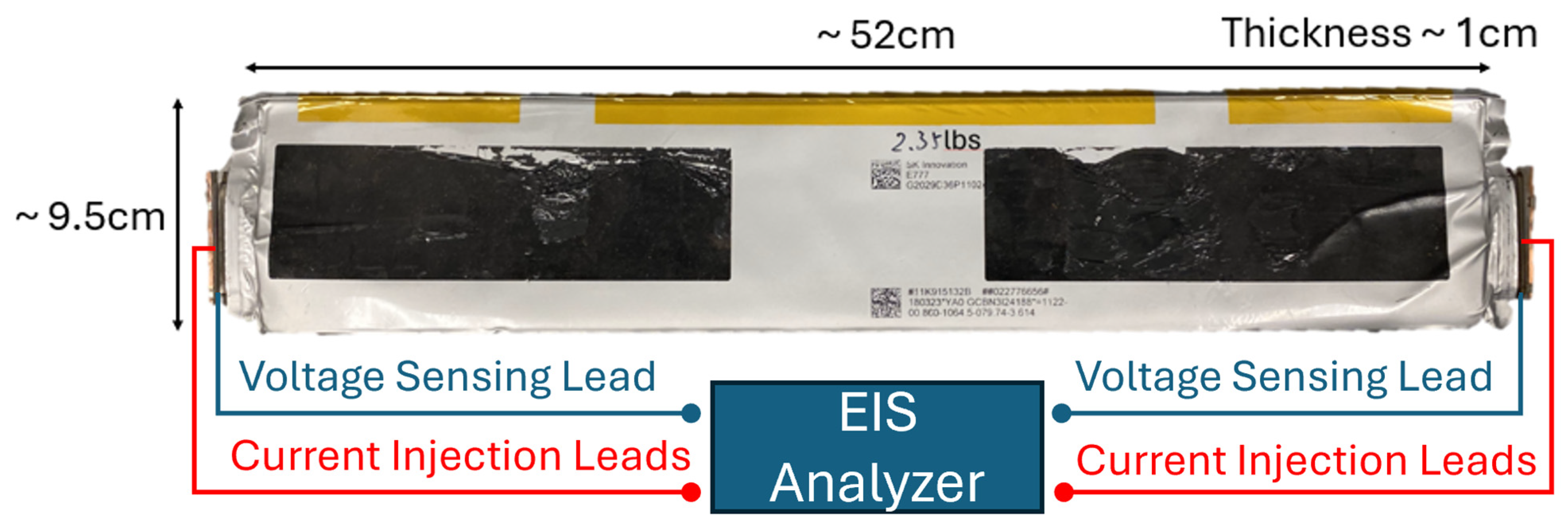
A large-format commercial lithium-ion pouch cell was obtained from a battery pack disassembled from an electric vehicle. [53]. Each cell weighs approximately 1.07   k g   ( 2.35   l b s . ) and measures 52 cm in length, 9.5 cm in width, and 1 cm in thickness, as shown in Figure 2. The EV cell has a nominal capacity of 78 Ah with a fully charged voltage of 4.15 V and a discharge cut-off voltage of 3.15 V. Cells were placed in a thermal chamber to maintain temperature stability during measurements. Thermocouples were used to measure the air and the cell temperature to ensure consistent temperature throughout the test. The state of charge, temperature, and number of repeated tests are summarized in Table 2.
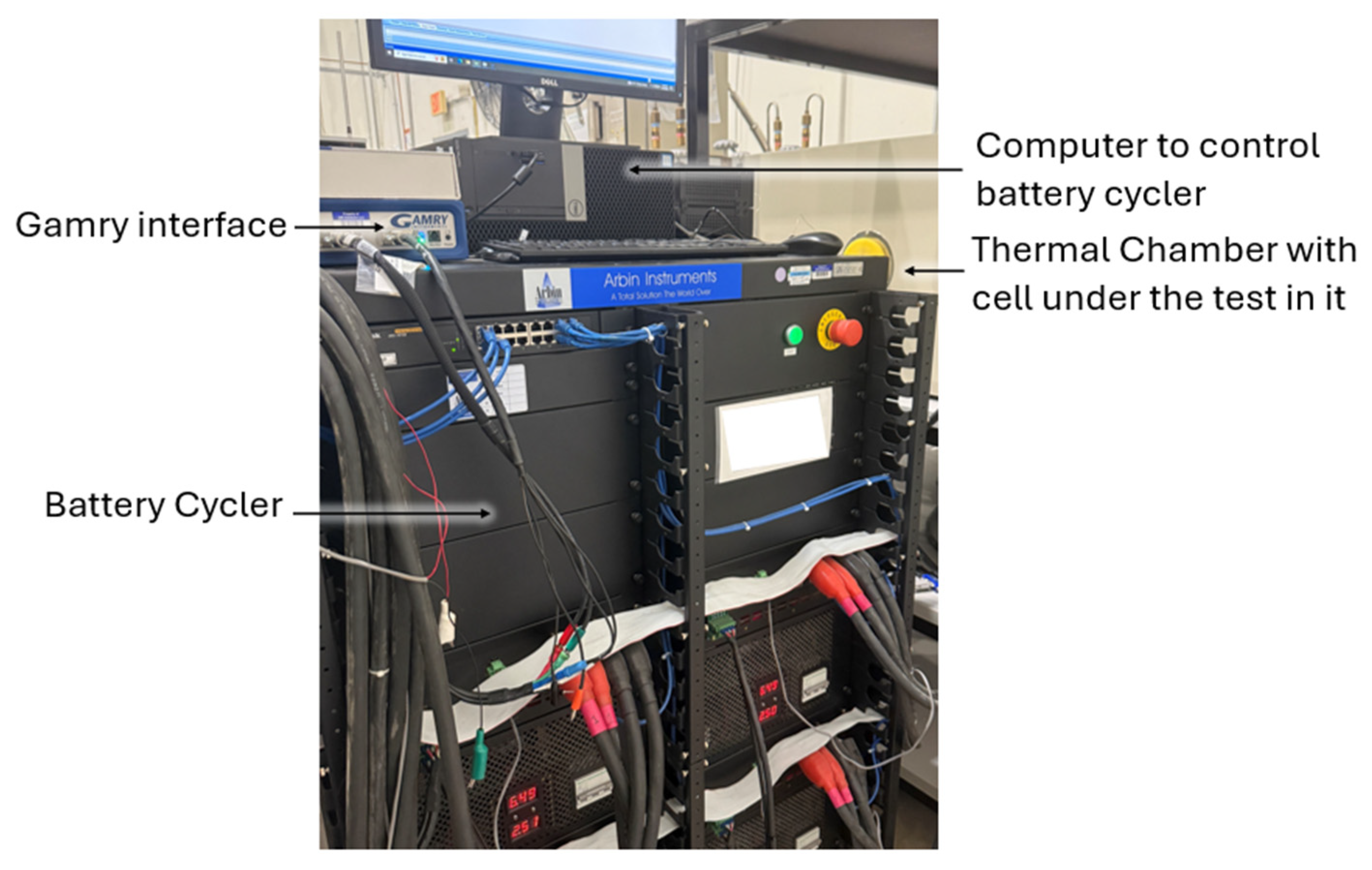
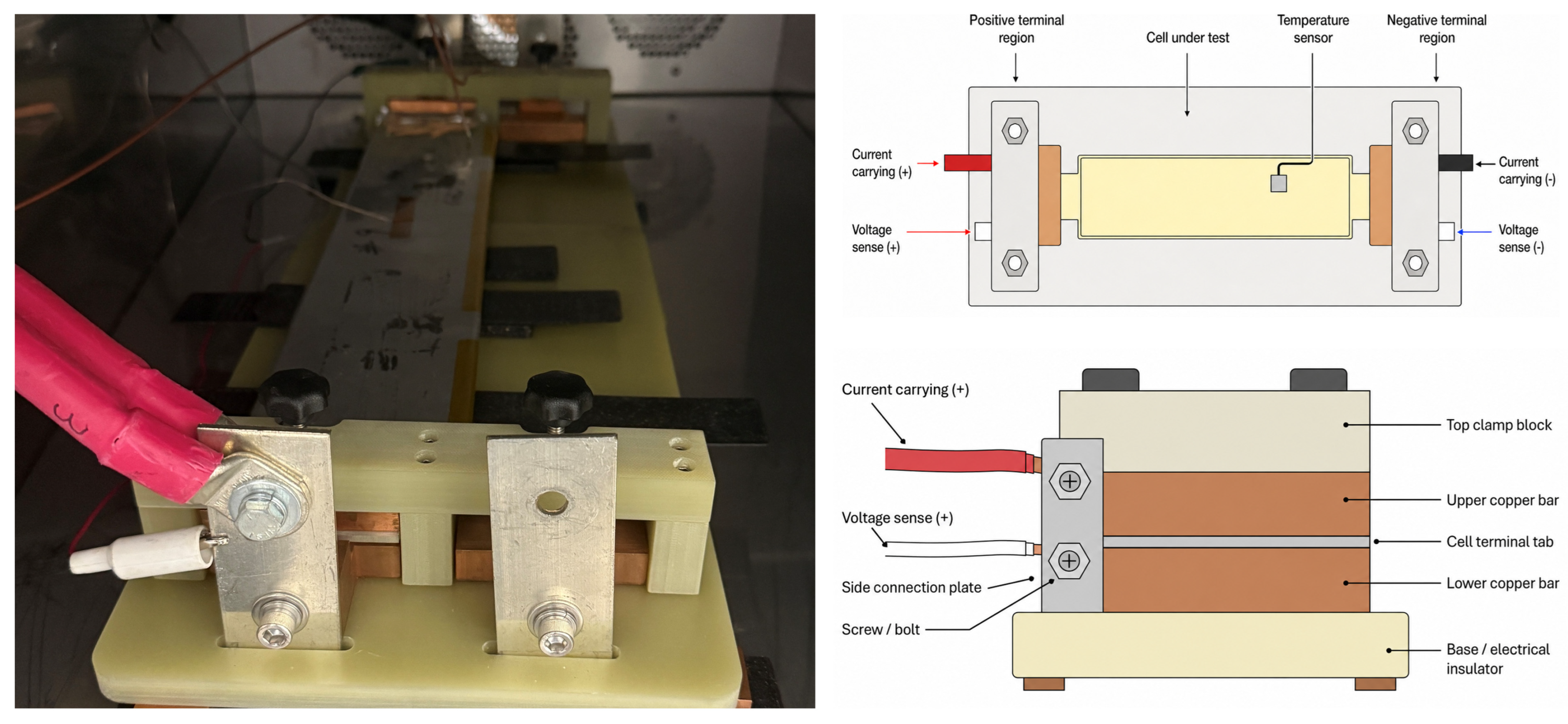
EIS tests were performed using a Gamry 5000P potentiostat/galvanostat (Gamry Instruments, Inc., Warminster, PA, USA) in conjunction with an Arbin battery cycler (500 A, 5 V) [54], as seen in Figure 3. EIS data were collected over a frequency range of 0.01 Hz to 10 kHz, with an amplitude of 1 mV.
Measurements were conducted using a four-terminal (Kelvin) configuration. Two leads were used to supply the current, and two separate leads were used to measure the voltage, as illustrated in Figure 2. The typical fixture designs are stated here:
(a)
A coaxial cable can be used as the test lead. Compared to solid core wires, coaxial cables exhibit lower inductance per unit length and maintain a consistent characteristic impedance. Their inherent shielding capability suppresses external electromagnetic interference while preserving signal integrity during measurements [29]. However, they generally have higher capacitance per unit length due to the closer proximity of the inner and outer conductors and the dielectric material within the cable, which should be considered in the design of the EIS analyzer.
(b)
Using thick solid core copper wire can reduce internal resistance and inductance [30].
(c)
Twisting the test lead can be used to cancel out inductance effects [16]. However, this approach can introduce repeatability issues, as maintaining a consistent twisting configuration across different tests is challenging. If the test lead is a coaxial cable, twisting can damage the cable’s shielding layer and add noise to the signal.
(d)
Shortening the test lead can also help, but it is generally unsuitable for coaxial cables, as shortening them may cause early signal reflections and introduce additional noise.
(e)
Minimizing the inductive effect of nearby metallic objects can further improve EIS measurement accuracy. A non-conductive test table, such as wood or plastic, is recommended [31]. The test leads also need to be as far apart as possible to minimize their mutual inductance effects [32].
(f)
Current-controlled (galvanostatic) mode is commonly recommended for a more accurate EIS measurement [32]. However, we observed that the galvanostatic mode can sometimes introduce additional errors in some EIS analyzers, likely arising from limitations in the feedback control accuracy to maintain a constant current. For low impedance measurement, the voltage-control (potentiostatic) mode can sometimes be more accurate.
(g)
A large excitation current can be used to enhance the magnitude of the response signal. This is achievable with an integrated or supplementary module of the EIS analyzer. However, using a large current may alter the cell configuration and violate the linearity assumption in classic EIS theory [33].
(h)
Minimizing the contact resistance between the battery and test leads is also critical, as the contact resistance is often the dominant source of EIS measurement errors. An alligator clip is not suitable for connecting the test subject to the EIS analyzer. The typical contact resistance between an alligator clip and the cell terminal is around 10 mΩ, which is an order of magnitude higher than the cell impedance of 1 mΩ. The contact resistance of an alligator clip can vary each time it is attached depending on the position where it is placed and the number of teeth in contact with the battery terminals. A specialized fixture is therefore required to connect the test leads to the battery for EIS measurement of ultra-low-impedance cells.
In the research, both the current injection and voltage measurement were connected to the battery’s positive and negative terminals with a custom fixture. In the original battery module, the cell terminals were laser-welded to a copper plate for electric connection. To disassemble cells from the module, the copper plate was cut, and the remaining sections attached to the cell were mechanically polished to obtain a flat surface in contact with the test fixture. The cell remained intact with its pouch unopened during the test. A regular open/short calibration was performed to remove parasitic contributions from the wiring and fixture: (1) Open calibration was conducted with no load attached, capturing the parasitic capacitance and inductance of the test leads and fixture. (2) Short calibration was performed by directly shorting the fixture terminals using a copper bar, allowing quantification of residual series resistance and inductance. The analyzer applies frequency-dependent compensation based on the open/short calibration to reduce residual contributions from the wiring and fixture. This procedure is particularly important for low-impedance measurements, where uncompensated series resistance and inductive contributions can be comparable to the measured cell response. This calibration procedure is particularly critical for low-impedance systems, where wiring and contact effects can otherwise exceed the intrinsic cell impedance. The custom connection fixture was designed as an adaptable four-terminal contact architecture for large-format pouch cells rather than as a standardized holder with fixed dimensions. In the present configuration, the testing leads in contact with be battery terminals were made from solid copper bar to improve surface contact using a screw-fastened clamping arrangement. The current-carrying leads and voltage-sensing leads were connected separately at the clamped terminal region to preserve the Kelvin sensing configuration and reduce the influence of lead and contact resistance on the measured impedance. The fixture was mounted on an electrically insulating base, and shims were used to maintain a stable and level contact geometry. Thermocouples were positioned to monitor both the cell and surrounding air temperatures during testing. Because commercial pouch cell terminal geometries and packaging dimensions vary substantially, the dimensions of the contact bars, screw spacing, and supporting structure can be adjusted to match the specific cell under investigation. The key design requirements are a large and stable metal-to-metal contact area, mechanically secure screw-fastened compression, separation of current and voltage-sensing paths, and electrical insulation of the terminal assembly. Open/short calibration was performed after assembly of the measurement pathway, with a copper bar used for short calibration to account for residual resistance and inductive contributions from the leads and the fixture. The diagram is shown in Figure 4. Following each SOC adjustment, the cell was rested under open-circuit conditions for 60 min before EIS measurement. A 15 min rest period was used between consecutive EIS tests with the same SOC and temperature. The open-circuit voltage (OCV) was recorded before each test, as seen in Table 2. For repeated tests at the same condition, the maximum OCV difference (ΔOCV) ranged from 3.2 to 9.9 mV across different SOC and temperature combinations. These rest periods were selected to balance measurement accuracy and test efficiency.
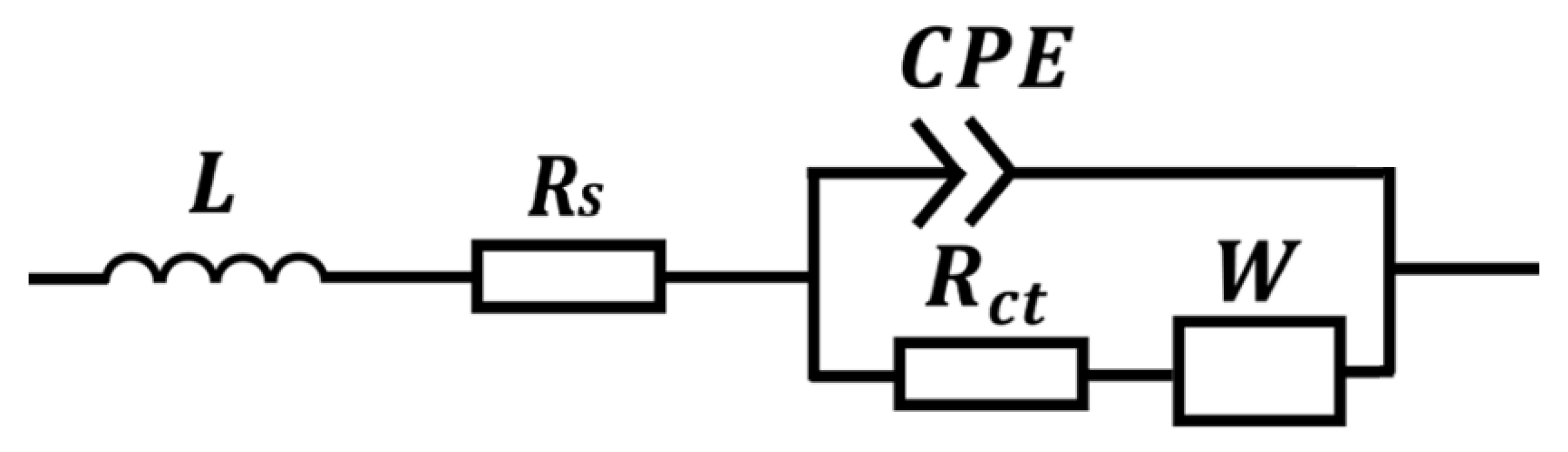
Following fixture-assisted EIS acquisition, the measured spectra were first assessed using the KK validity test and subsequently interpreted using the ECM shown in Figure 5.

2.2. Kramers–Kronig Validation

For a linear, causal, stable, and time-invariant electrochemical system, the real and imaginary parts of the impedance are not independent but are linked by the Kramers–Kronig (KK) relations. Agreement between the measured and KK-reconstructed spectra provides a consistency check for the quality of the EIS data under the assumptions of linearity, causality, stability, and time invariance. The Kramers–Kronig relations are a set of integral transforms connecting the real and imaginary parts of any linear, causal, and stable system’s impedance:
Re Z ω = Z + 2 π P 0 ω   Im Z ω ω 2 ω 2 d ω
Im [ Z ( ω ) ] = 2 ω π P 0 Re [ Z ( ω ) ] Z ω 2 ω 2 d ω
where Z   is a real number that corresponds to the ohmic resistance of the system. P denotes the Cauchy principal value. Direct application of these integrals is sensitive to noise, frequency truncation, and the number of frequency points used in the EIS measurement. Schönleber et al. proposed a robust linear KK approach, providing a practical validation method for battery EIS data [55]. The implementation of his method is briefly summarized here: the battery impedance is expressed as a series connection of N R C parallel RC branches, where each RC branch corresponds to a characteristic time constant, plus a series resistance R and optional inductance L :
Z ( ω ) = R + k = 1 N R C R k 1 + j ω τ k + j ω L
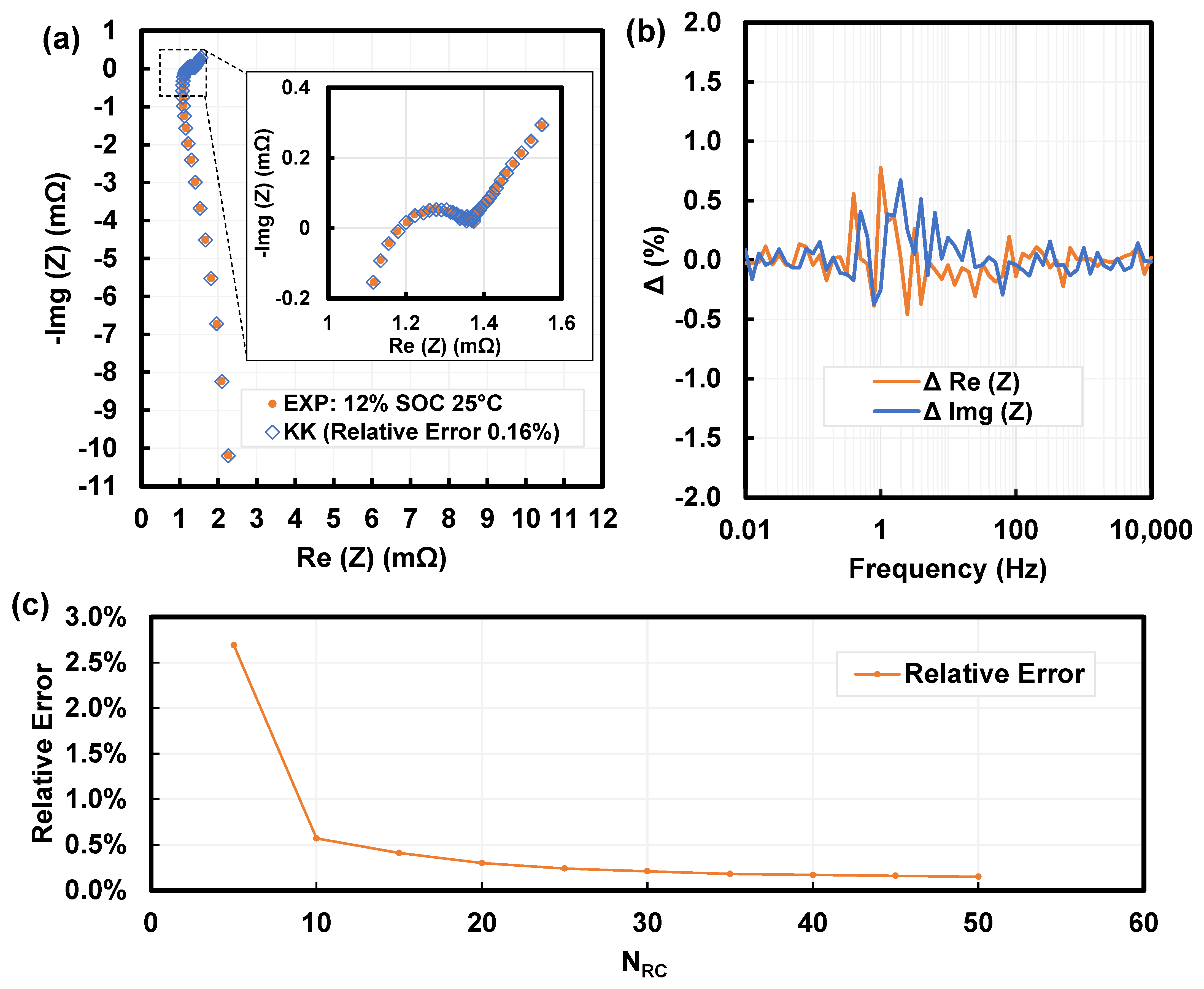
where Z ω is the complex impedance of the system with respect to frequency ω . R k is the resistance of the k -th RC element, τ k is the corresponding time constant, and L is the inductance that is used to capture high-frequency inductive effects. j = 1 is the imaginary unit. The capacity value C k = τ k / R k in each RC branch is determined by the time constants τ k . Notice τ k should be logarithmically spaced across the measured frequency range. An insufficient number of RC elements ( N R C ) may leads to underfitting of the impedance data, while an excessive N R C may overfit measurement noise, resulting in misleading residuals in both cases. In this work, we adopted N R C = 50 as a practical balance. It is seen that the KK fit result does not have obvious underfitting or overfitting, as shown in Figure 6 and Appendix A.
τ k = τ min τ max τ min k 1 N 1
τ m i n = 1 / ω m a x and   τ m a x = 1 / ω m i n
Let Z e x p = R e Z e x p + j I m Z e x p be the measured impedance in experiment. Z e x p , 1 , Z e x p , 1 , Z e x p , N e x p denotes the total N e x p sampled frequency in the test data.
Define a linear system:
b = A x
With:
b = R e Z e x p , 1 , I m Z e x p , 1   ,   R e Z e x p , N , I m   Z e x p , N T
x = [ R , L , R 1 , , R N ] T
A = 1 0 ϕ 1 ( ω 1 ) ϕ N ( ω 1 ) 0 ω 1 ϕ 1 ( ω 1 ) ϕ N ( ω 1 ) 1 0 ϕ 1 ( ω M ) ϕ N ( ω M ) 0 ω M ϕ 1 ( ω M ) ϕ N ( ω M )
where:
ϕ k ω i =   R e ϕ k ω i = 1 1 + ( ω i τ k ) 2
ϕ k ω i = I m ϕ k ( ω i ) = ω i τ k 1 + ( ω i τ k ) 2
The linear system is solved using regularized least squares to find x :
x = a r g   m i n x   A x b 2
And the fitted x is used to compute the KK-consistent impedance Z K K . The real and imaginary residuals quantify the deviation from KK consistency:
Δ Z = Re [ Z exp ] Re [ Z KK ]
Δ Z = Im [ Z exp ] Im [ Z KK ]
Relative residual norm is defined as:
r e l _ e r r o r = [ Δ Z ; Δ Z ] 2 [ R e [ Z e x p ] ; I m [ Z e x p ] ] 2
Percentage residuals can also be calculated:
Z % = 100 Δ Z Re [ Z exp ] , Δ Z % = 100 Δ Z Im [ Z exp ]
This allows the assessment of EIS data quality.

2.3. EIS Equivalent Circuit Parameter Identification

Accurate identification of equivalent circuit model parameters with clear physical meaning is essential for interpreting EIS data. To maintain model simplicity and interpretability, ECM parameters were kept constant across different states of charge and temperatures whenever feasible.
The selected ECM, consisting of a series inductance and solution resistance followed by a CPE in parallel with a charge-transfer resistance/generalized Warburg branch, was chosen according to the characteristic features of the measured spectra, shown in Figure 5. A classical Randles-type model with an ideal double-layer capacitor and ideal semi-infinite Warburg element would not explicitly represent the depressed semicircular response and the approximately 60° low-frequency diffusion-related tail observed in the present spectra. Therefore, the ideal capacitor was replaced with a CPE to represent non-ideal interfacial behavior, while a generalized Warburg element was adopted to describe the non-ideal diffusion response. A series inductance was retained to account for the high-frequency inductive contribution associated with the low-impedance cell measurement configuration. In addition, no separate SEI-related RC branch was introduced because no clearly distinguishable second semicircle was resolved in the measured spectra. Nevertheless, the selected ECM should be interpreted as an effective lumped representation rather than a unique mechanistic decomposition, since different circuit topologies may produce similar fitting quality over a limited frequency range. The impedance equation and ECM diagram are shown in Table 3 and Figure 5.
The data used for ECM fitting covered a frequency range from 0.01   H z to 251   H z . Notice that the effective series inductance L need to be included in ECM of low-impedance EV-cell. This is because the inductive contributions from the cell terminals, large metallic current collectors, fixture–cell interconnections, and measurement leads can be comparable in magnitude to the milliohm-scale impedance response of the cell. This inductive segment is not interpreted as an electrode–electrolyte interfacial process.
Bayesian optimization was employed to identify the global optimum of the ECM parameters [56]. Once the global solution was obtained, it was further refined using Nelder–Mead simplex method [57], a local optimization technique. Bayesian optimization was implemented using an open-source library [58], while the Nelder–Mead simplex method was executed via the SciPy [59] package.
The Gaussian process used in BO is defined as:
f θ ~ N m θ , k θ , θ
where m θ is the prior mean function, and k θ , θ is the covariance between θ and θ . In this work, the prior mean is set to zero, which is a common and practical assumption when the true mean is unknown. The corresponding covariance matrix is given in Equation (18). The covariance matrix is constructed using Matérn kernel, which is embedded in the open-source implementation. In this work, θ is a vector of model parameter, for example L ,   R s , R c t , Q , α , R w , T , γ / 2 .
Since the prior meaning is not known, then we simply assume the prior mean is zero, which is a practical procedure [60]. The Gaussian process exhibits the useful property that any new point θ t + 1 is joint Gaussian with f t + 1 = f ( θ t + 1 ), which implies:
f 1 : t f t + 1   ~   N   0 , K k k T k ( θ t + 1 , θ t + 1 )
where:
K = k ( θ 1 , θ 1 ) k ( θ 1 , θ t ) k ( θ t , θ 1 ) k ( θ t , θ t )
and:
k = [ k θ t + 1 , θ 1   k θ t + 1 , θ 2 k ( θ t + 1 , θ t ) ] T
For Gaussian processes (GPs), the predictive probabilistic surrogate distribution at unexplored locations in the domain is given. Following the procedure of Rasmussen et al. [61], the probabilistic surrogate distribution for unexplored locations is given by:
P   ( f t + 1   |   D t + 1 , θ t + 1 )   ~   N   ( u ( θ t + 1 ) ,   σ 2 ( θ t + 1 ) )
where:
u ( θ t + 1 )   =   k T K 1 f 1 : t
and:
σ 2 ( θ t + 1 )   =   k ( θ t + 1 , θ t + 1 )     k T K 1   k .
To find the next sampling point θ t + 1 , the lower confidence bounds (LCBs) are optimized by Equation (24), where κ is the hyperparameter to balance the exploration and exploitation:
α L C B =   u ( θ t + 1 )     κ   σ ( θ t + 1 )
Root mean squared error (RMSE) is used as the residual metric to quantify the difference between theorical model and the experimental data. The detailed Bayesian and Nelder–Mead optimization implementation follows the procedure documented in the literature [62].

3. Result

3.1. EIS Experimental Data Kramers–Kronig Validity

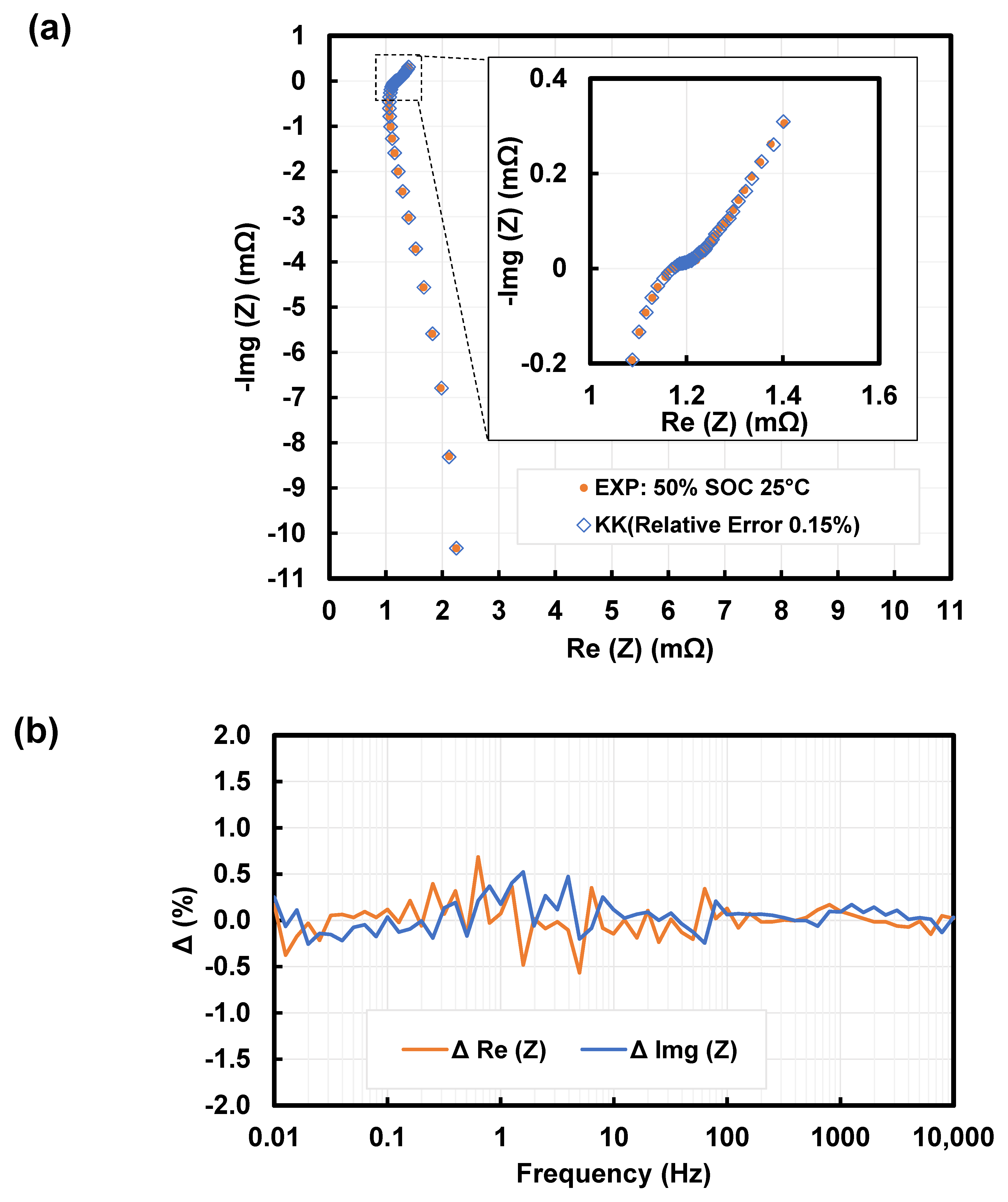
The linear Kramers–Kronig (KK) validity test is performed for all experimental data [55]. As seen in Figure 6 and in Appendix A, KK-reconstructed impedance closely matches the measured data in the Nyquist plot. The overall relative error for the KK result is around 0.15%. The maximum residual over the measured frequency range remains within ±0.5% for both the real and imaginary components. These results indicate that the measured spectra are consistent with the KK requirements over the entire frequency range (0.1 Hz–10 kHz). Minor biased trends are observed in the mid-frequency range (0.1 Hz–10 Hz); However, the relative error associated with KK compliance remains very small. Considering the low impedance magnitude of the cell (on the order of 1 mΩ), the observed deviations are considered acceptable. The Nyquist overlays in this subsection are provided only to visualize the agreement between the measured and KK-reconstructed impedance spectra. KK compliance is assessed quantitatively using the real and imaginary residuals and the overall relative error; no geometric interpretation of the Nyquist response is made from these validation plots.

3.2. EIS Experimental Data and Fitting Result

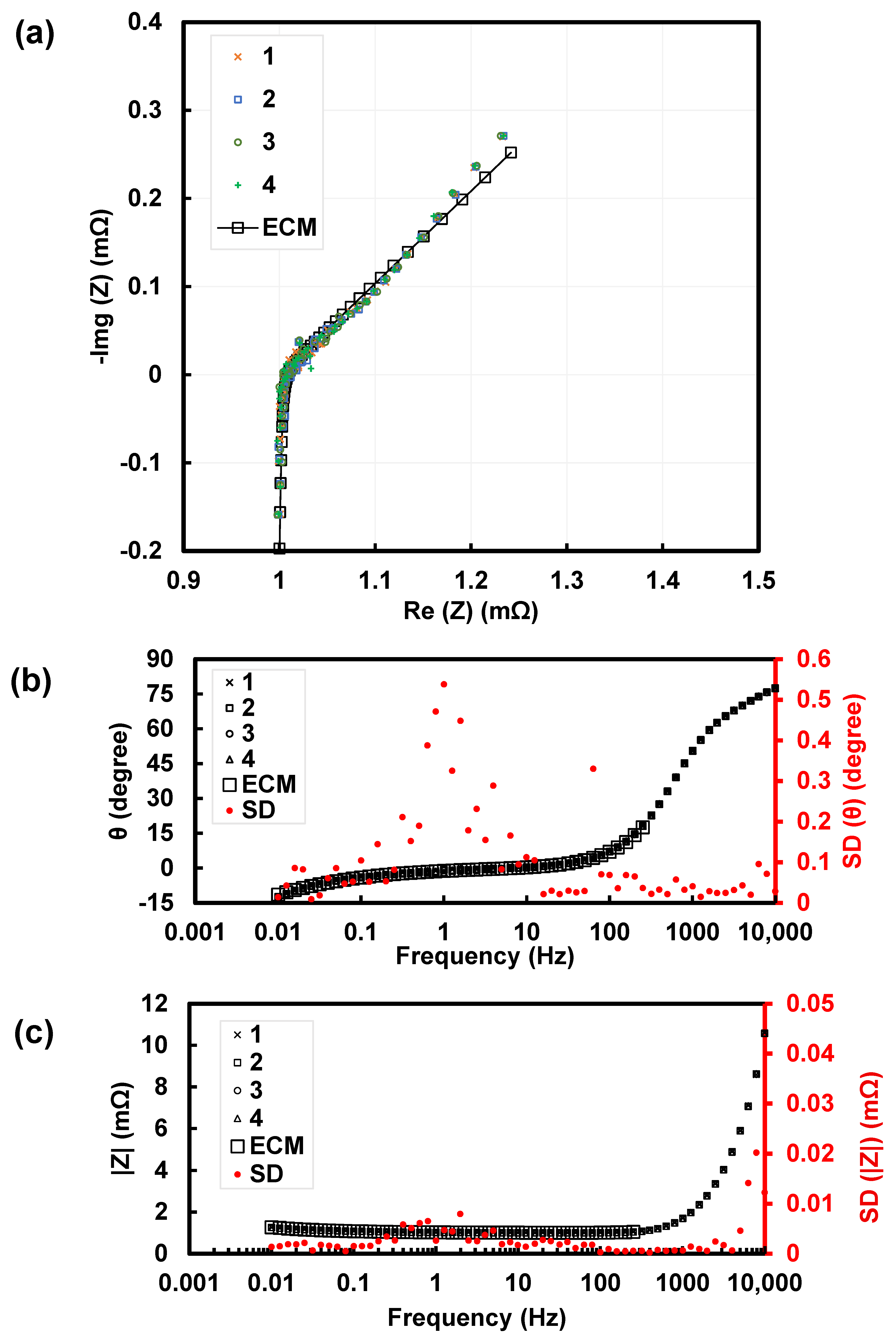
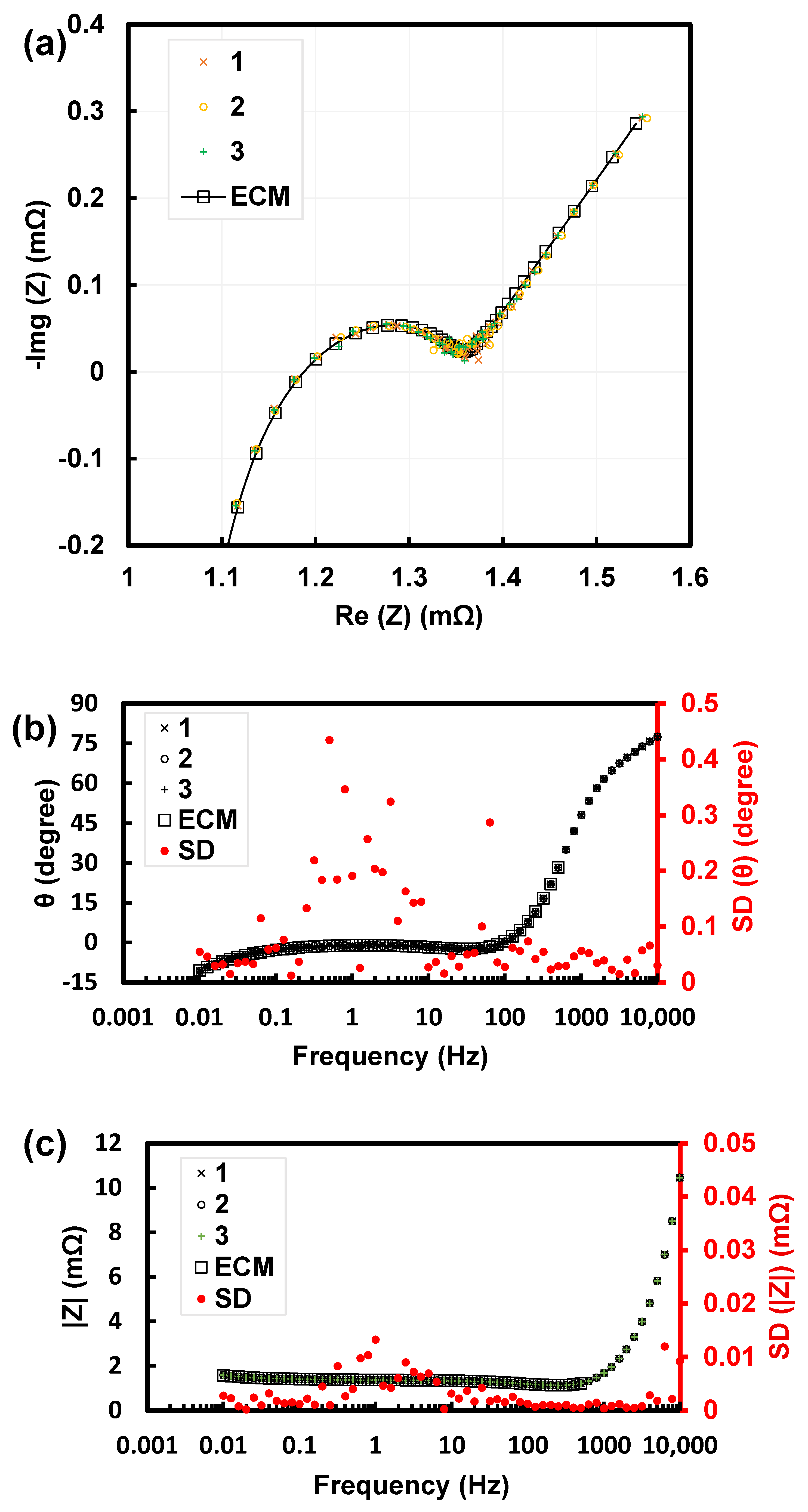
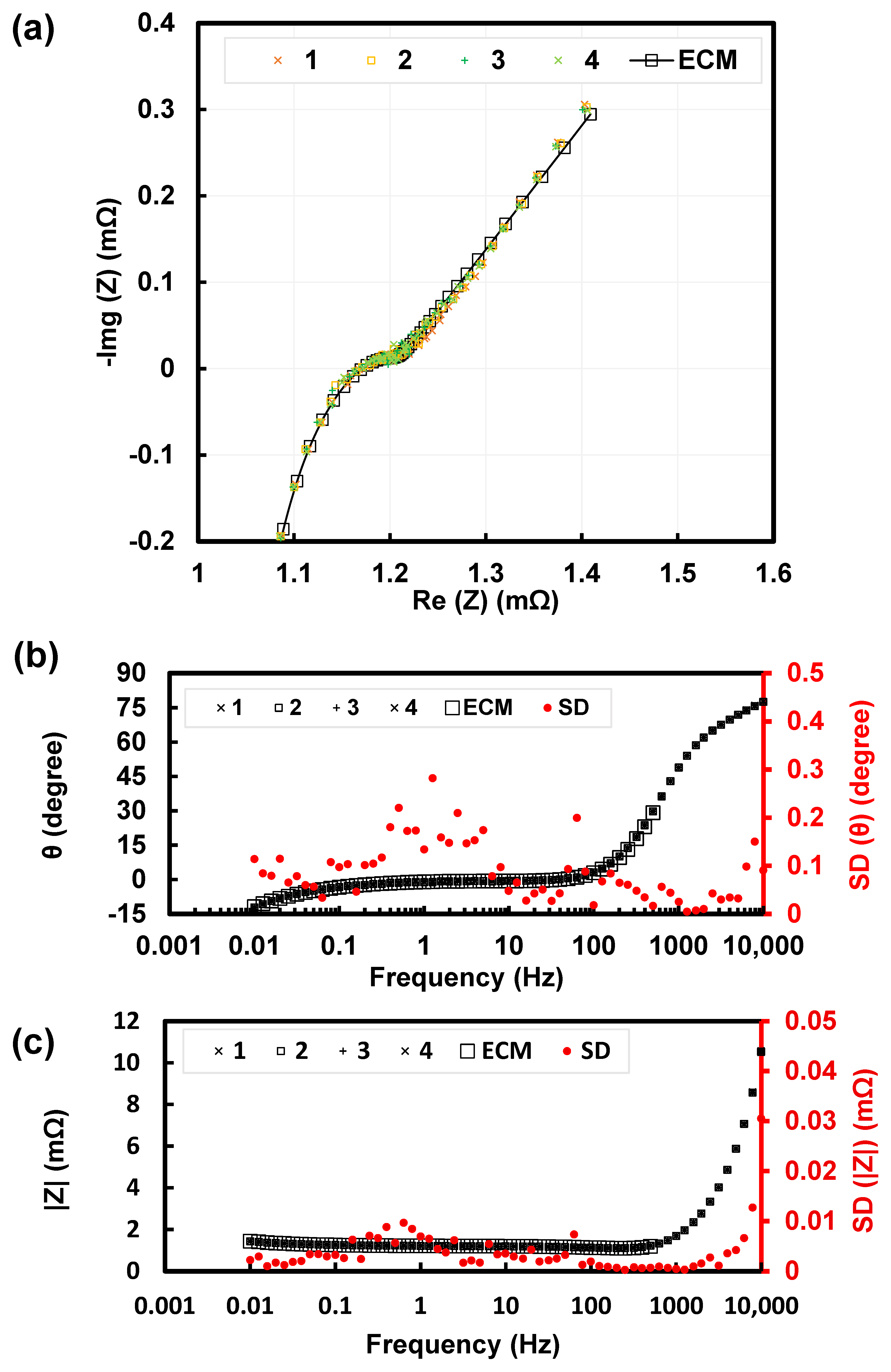
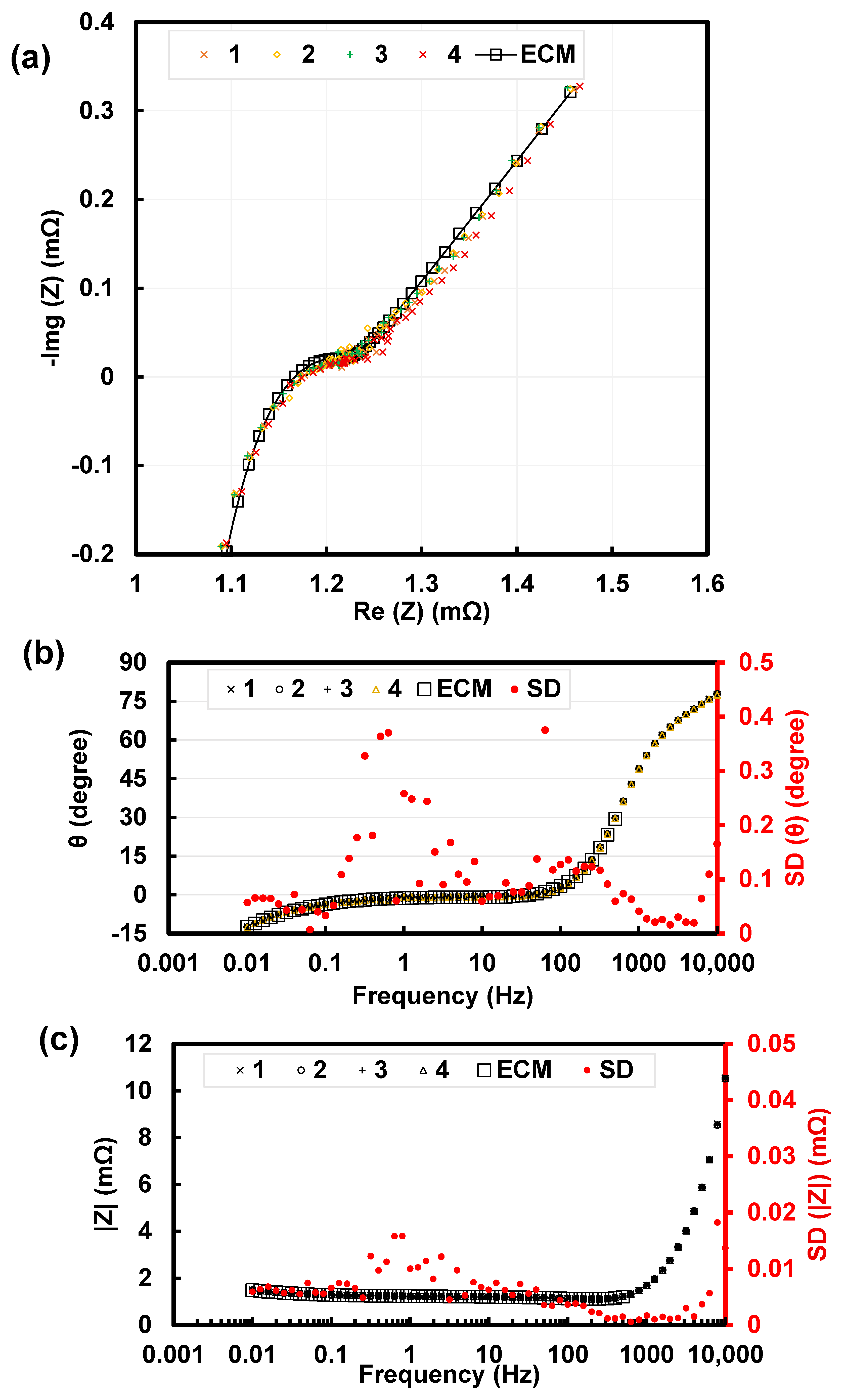
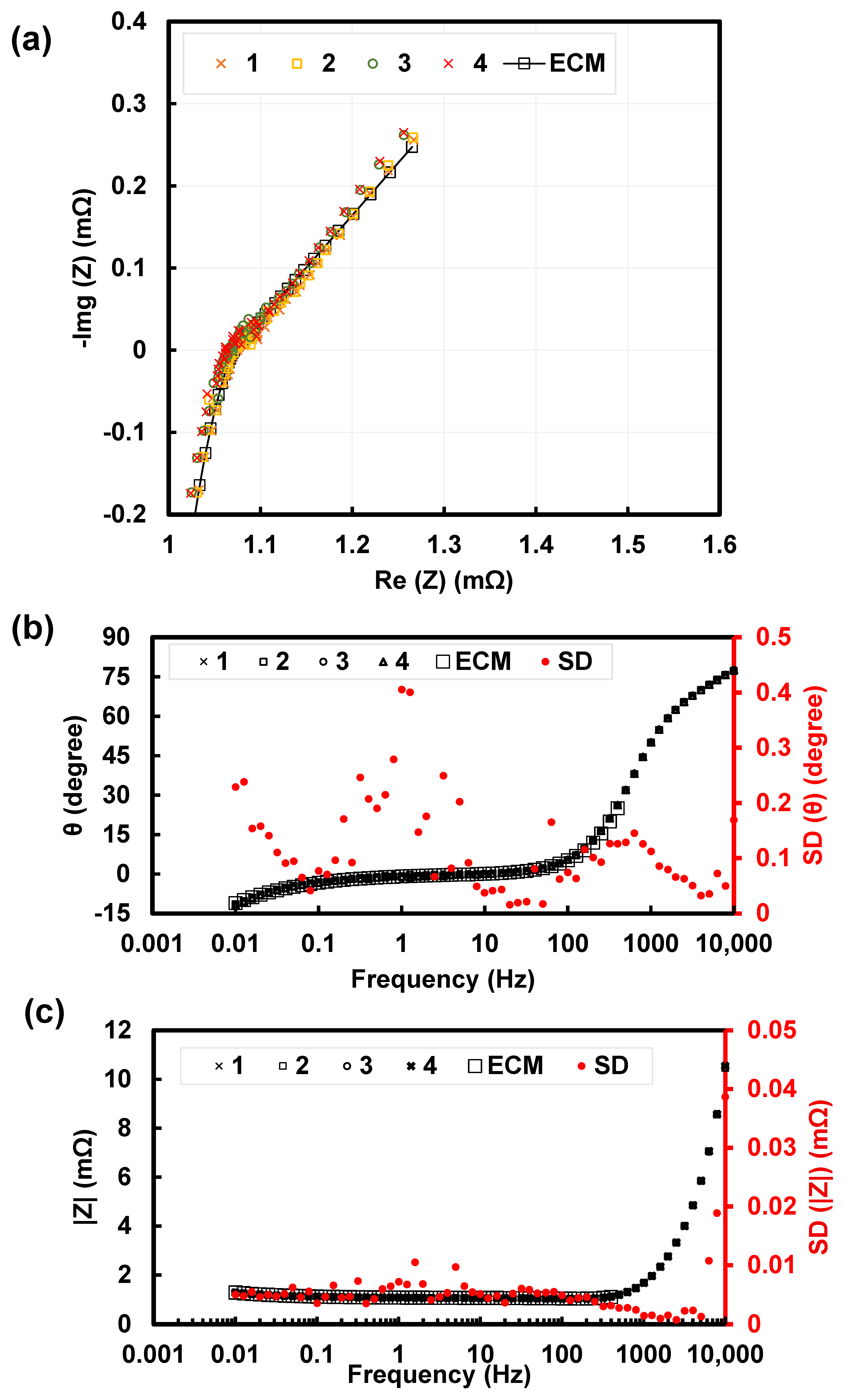
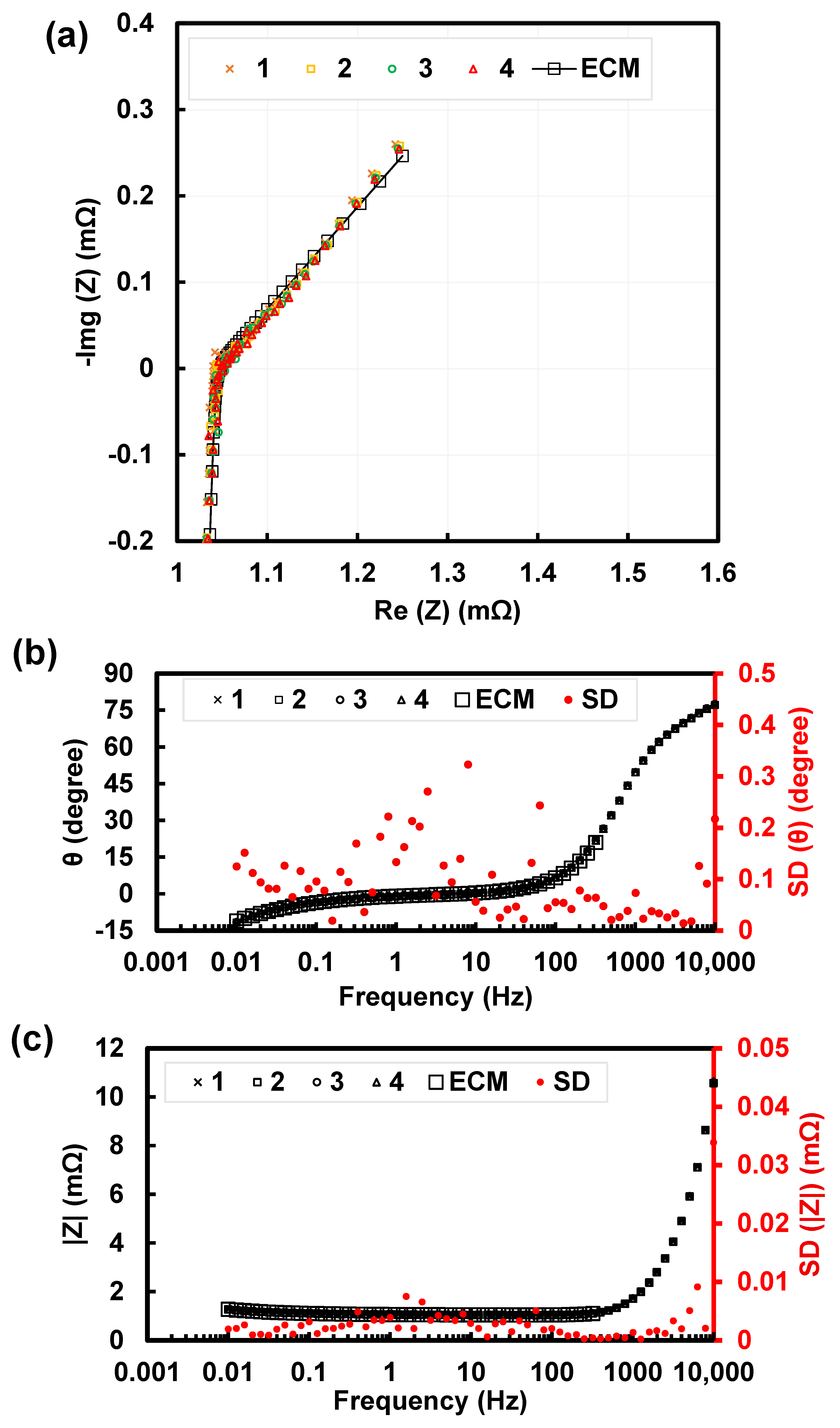
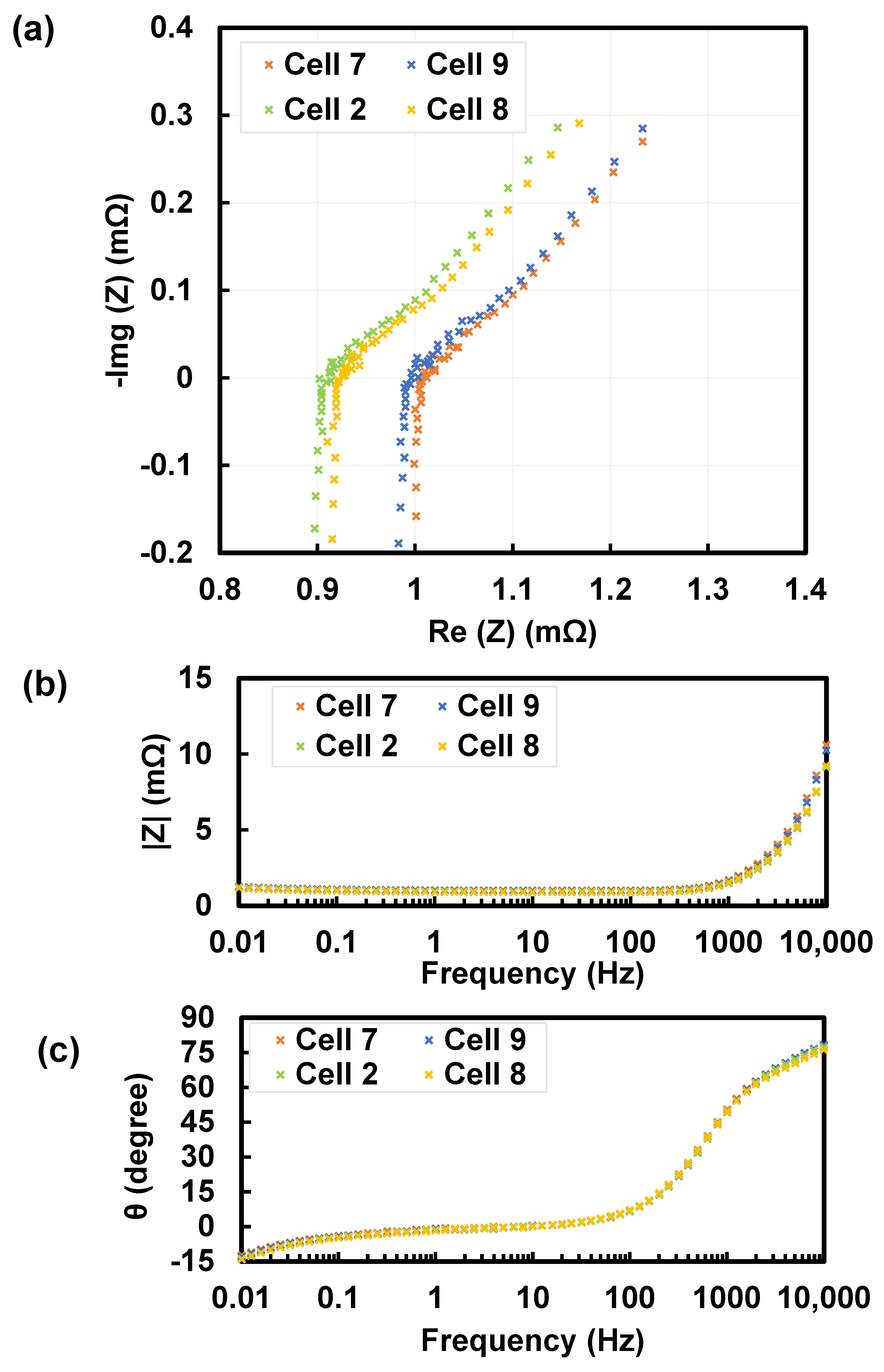
EV cells were tested under the following SOC and temperature conditions, as summarized in Table 2: 12% SOC at 25 °C, 50% SOC at 25 °C, 100% SOC at 25 °C, 50% SOC at 40 °C, and 100% SOC at 40 °C. The corresponding impedance spectrum is shown in Figure 7, Figure 8, Figure 9, Figure 10, Figure 11 and Figure 12, respectively. The numbers in the figure refer to the number of repeated tests conducted on the same cell under identical test conditions. To evaluate the test repeatability, at each frequency point j , the standard deviation (SD) of magnitude and phase angle are calculated as:
S D Z ( j ) = 1 n i = 1 n Z i j Z ¯ i j 2 ,   where   Z ¯ i j 1 n i = 1 n Z i ( j )
S D θ ( j ) = 1 n i = 1 n θ i ( j ) θ ¯ ( j ) 2 ,   where   θ ¯ ( j ) 1 n i = 1 n θ i ( j )
where Z i ( j ) and θ i ( j ) are the impedance magnitude and phase angle values from the i -th repeated test at frequency point j , Z ( j ) and θ ¯ ( j ) are the mean values at frequency point j , and n = 4 is the number of repeated tests. The standard deviation at each frequency is shown in Figure 7, Figure 8, Figure 9, Figure 10, Figure 11 and Figure 12. The maximum standard deviation for the phase angle and magnitude is below 0.1 ° and 0.05 mΩ, respectively, across all frequencies. We observe that the part of the test data at higher frequencies (251 Hz–10 kHz) still has very good repeatability.
The average standard deviation for magnitude and phase angle across all frequency points is:
S D ¯ Z = 1 m j = 1 m s Z ( j )
S D ¯ θ = 1 m j = 1 m s θ j
where m = 61 is the total number of frequency sampling points, S D ¯ Z represents the average standard deviation of impedance magnitude (in mΩ), and S D ¯ θ represents the average standard deviation of phase angle (in degrees). These values are summarized in Table 4. The small standard deviation of phase angle and magnitude among repeated tests demonstrated excellent repeatability of the test data, as shown in Figure 7, Figure 8, Figure 9, Figure 10, Figure 11 and Figure 12.
In a Nyquist plot, the positive of the y-axis typically represents the negative imaginary component of the impedance. Therefore, the upper half of the Nyquist plot corresponds to capacitive behavior, while the lower half indicates inductive behavior. Part (b) and (c) display the Bode plots, where the phase angle and magnitude are plotted as functions of frequency, respectively. The fitted spectra include the response from 0.01   H z up to 251   H z . In this range, the measured impedance has entered the negative imaginary region, allowing the series inductance term in the ECM to be identified. Because the impedance magnitude of the tested EV pouch cell is in the sub-milliohm to milliohm range, this inductive contribution is non-negligible for accurate representation of the measured spectrum. Nevertheless, the inductive segment is treated as an effective high-frequency electrical contribution and is not used to infer charge-transfer or diffusion-related electrochemical behavior.
For the 12% SOC at 25 °C case, the tested frequency range spans from 0.01   H z to 10   k H z , as shown in the Bode plots in Figure 7. In the Nyquist plots, the imaginary axis begins at approximately 0.2   m . The Nyquist curve intersects the real axis at around 125   H z , marking the beginning of a semicircular arc. The peak of the semicircle corresponds to a frequency between 20   H z and 30   H z , and the arc terminates near 1   H z . Beyond this point, the curve transitions into a straight line, representing the Warburg diffusion element. Due to the presence of inductance in our model, the entire diagram is shifted downward, placing the center of the semicircle below the real axis. In Nyquist plots, the battery response progresses from high to low frequency as the data points move from the lower left to the upper right along the curve. Approximately, the intersection of the semicircle to the real axis represents the solution resistance, while the diameter for the semicircle corresponds to the charge-transfer resistance. The fitted values of T are substantially larger than the characteristic times normally associated with solid-state lithium-ion diffusion. In the generalized Warburg expression used here, T determines the frequency scale through the product ω T . For the fitted values reported in Table 5, the corresponding finite-length transition lies far below the measured frequency range. Consequently, the generalized Warburg element remains close to its fractional power-law regime over the available data. The linear segment in the upper right indicates the generalized Warburg diffusion process at low frequencies. The classical semi-infinite Warburg diffusion is represented by a line at 45° at lower frequency. However, in our case, the line is approximately 60°. This phenomenon is believed to be caused by diffusion in the porous electrodes [35]; similar behavior has also been reported in high-capacity commercial lithium-ion batteries [63]. Further investigation is needed to fully explain this phenomenon.
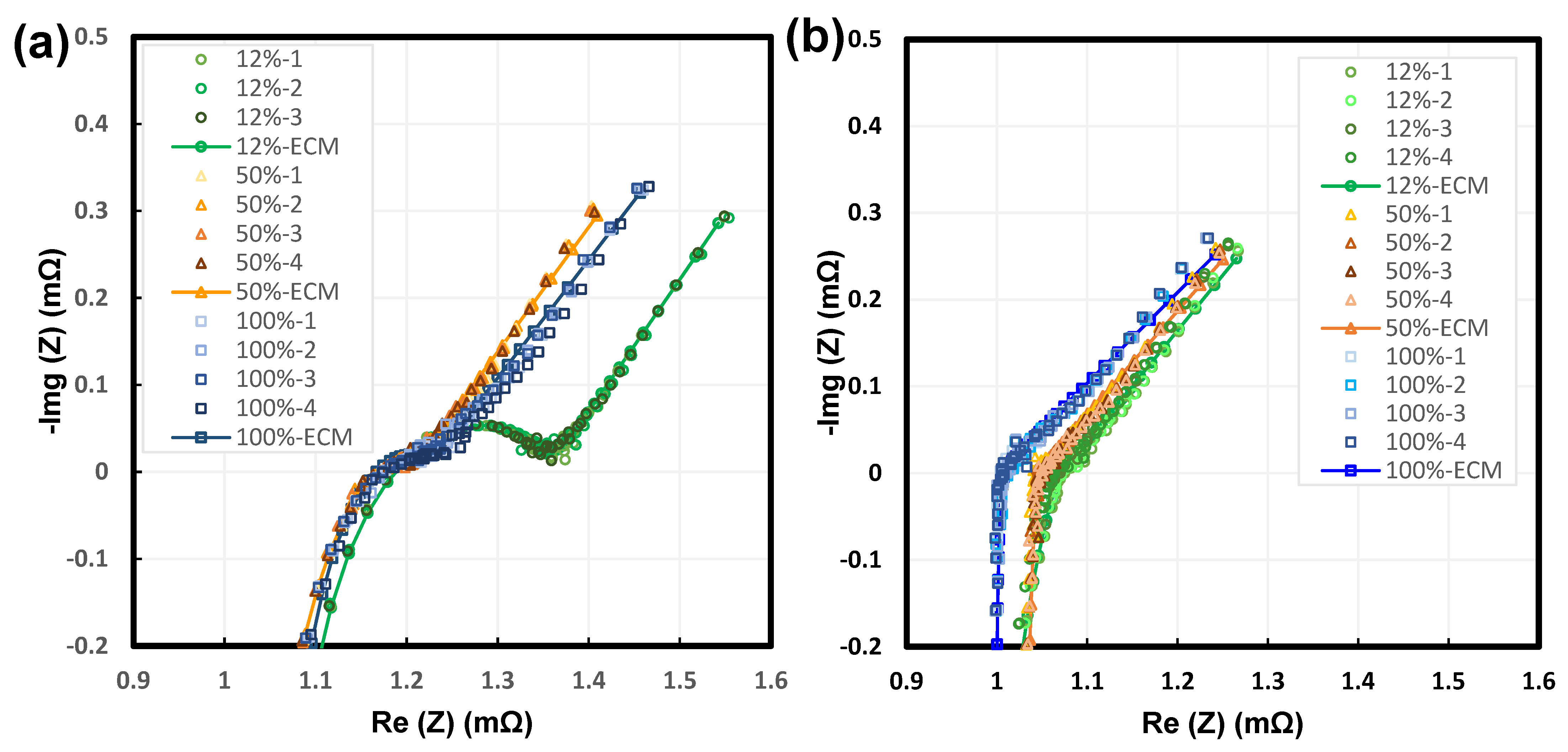
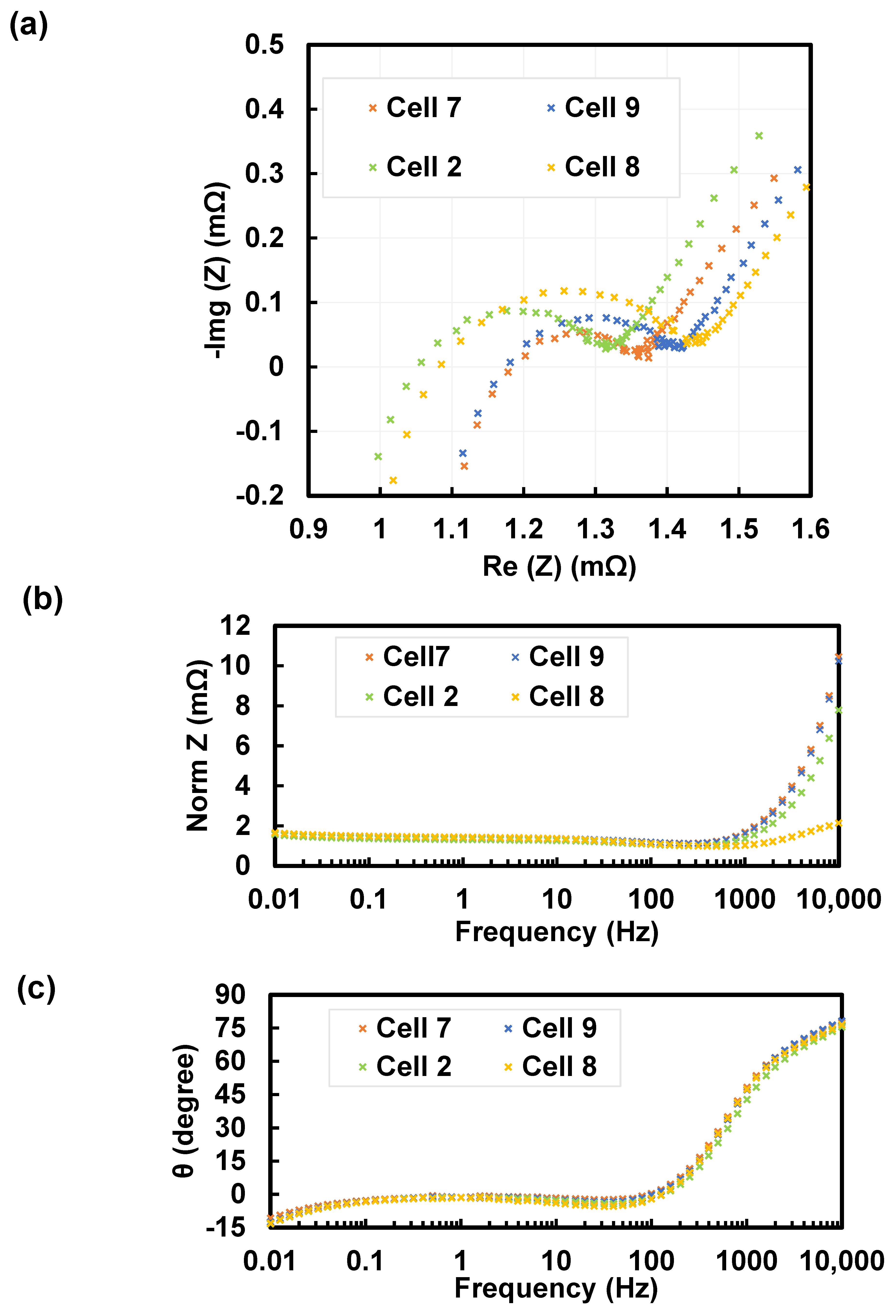
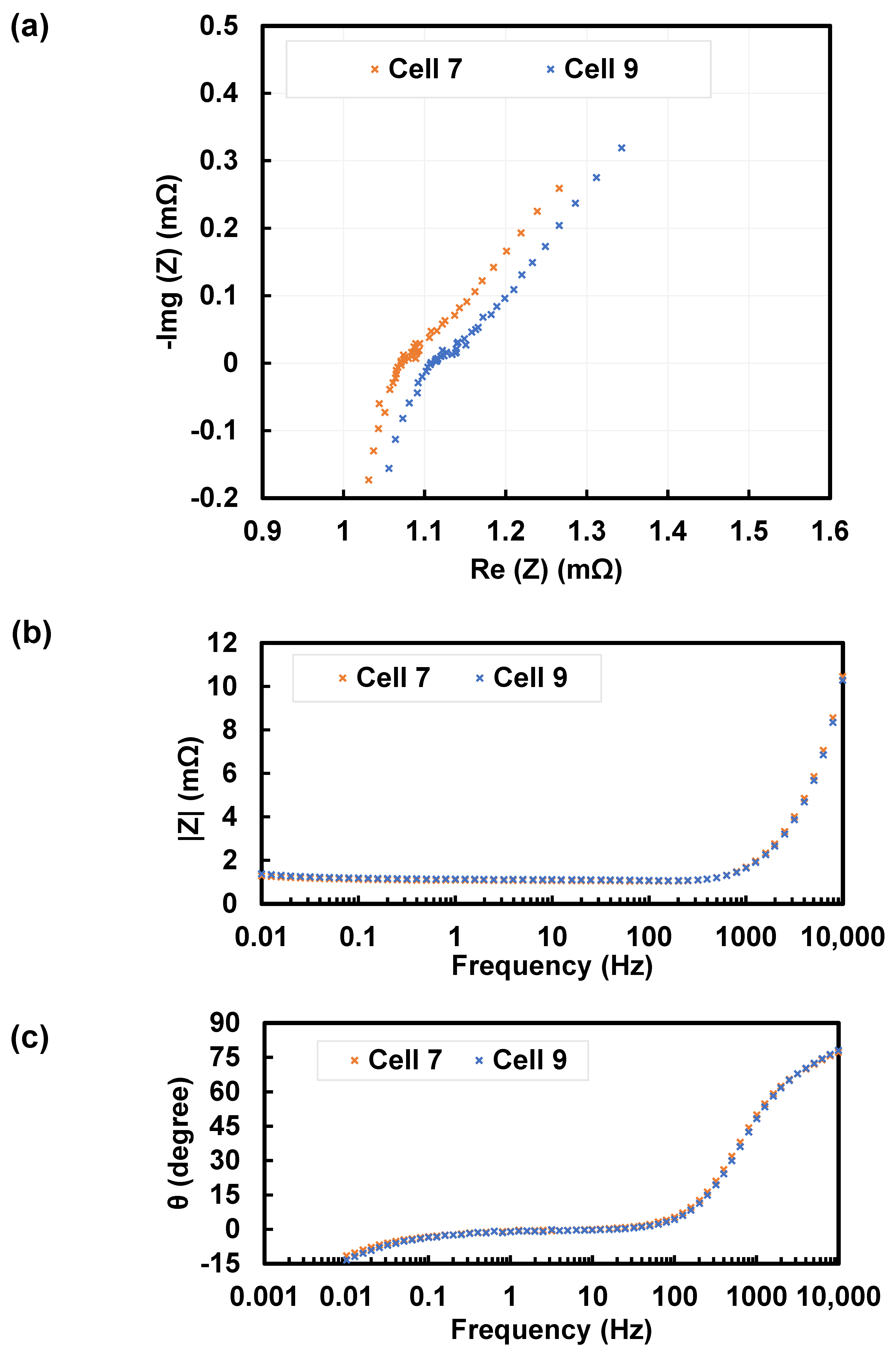
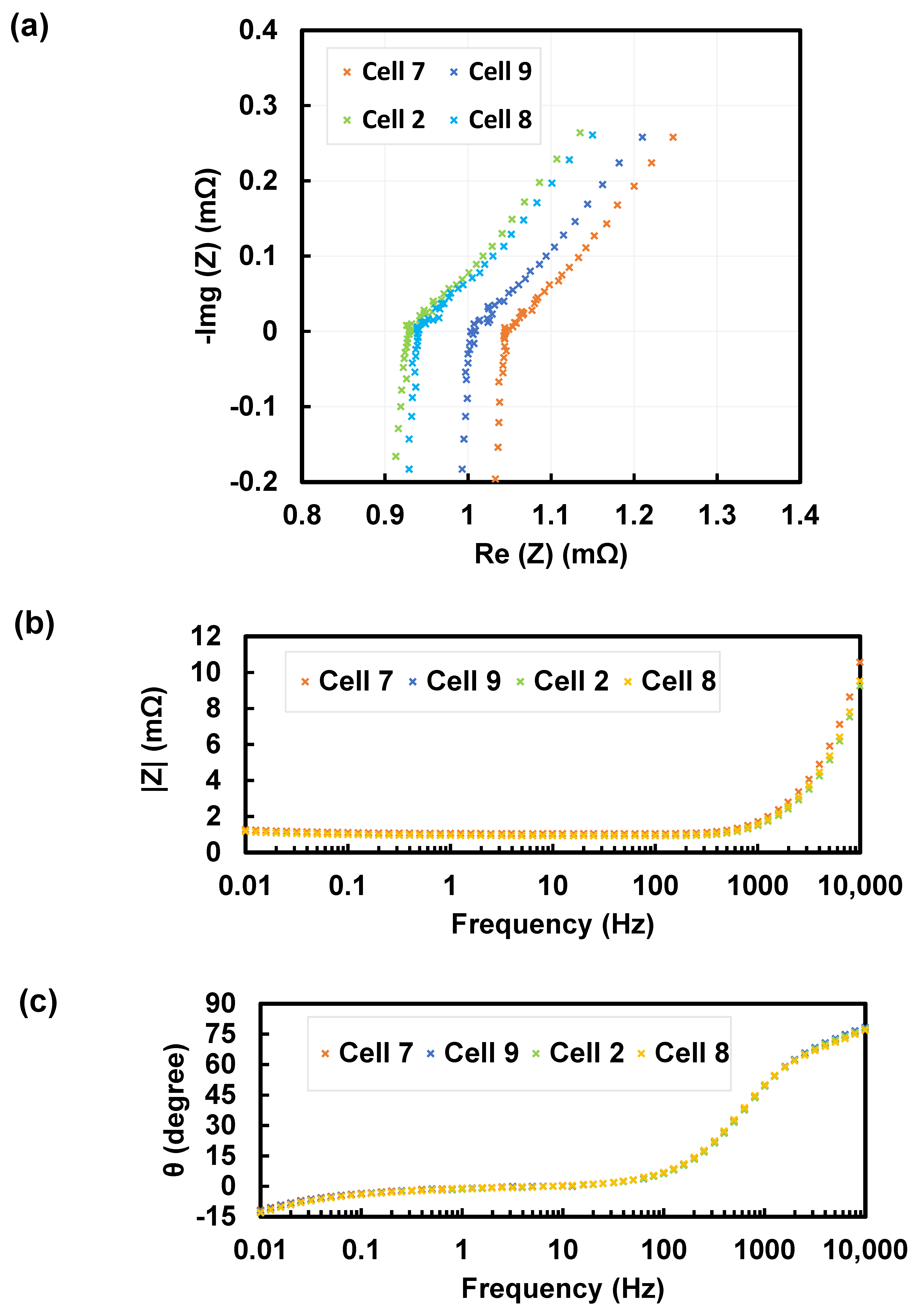
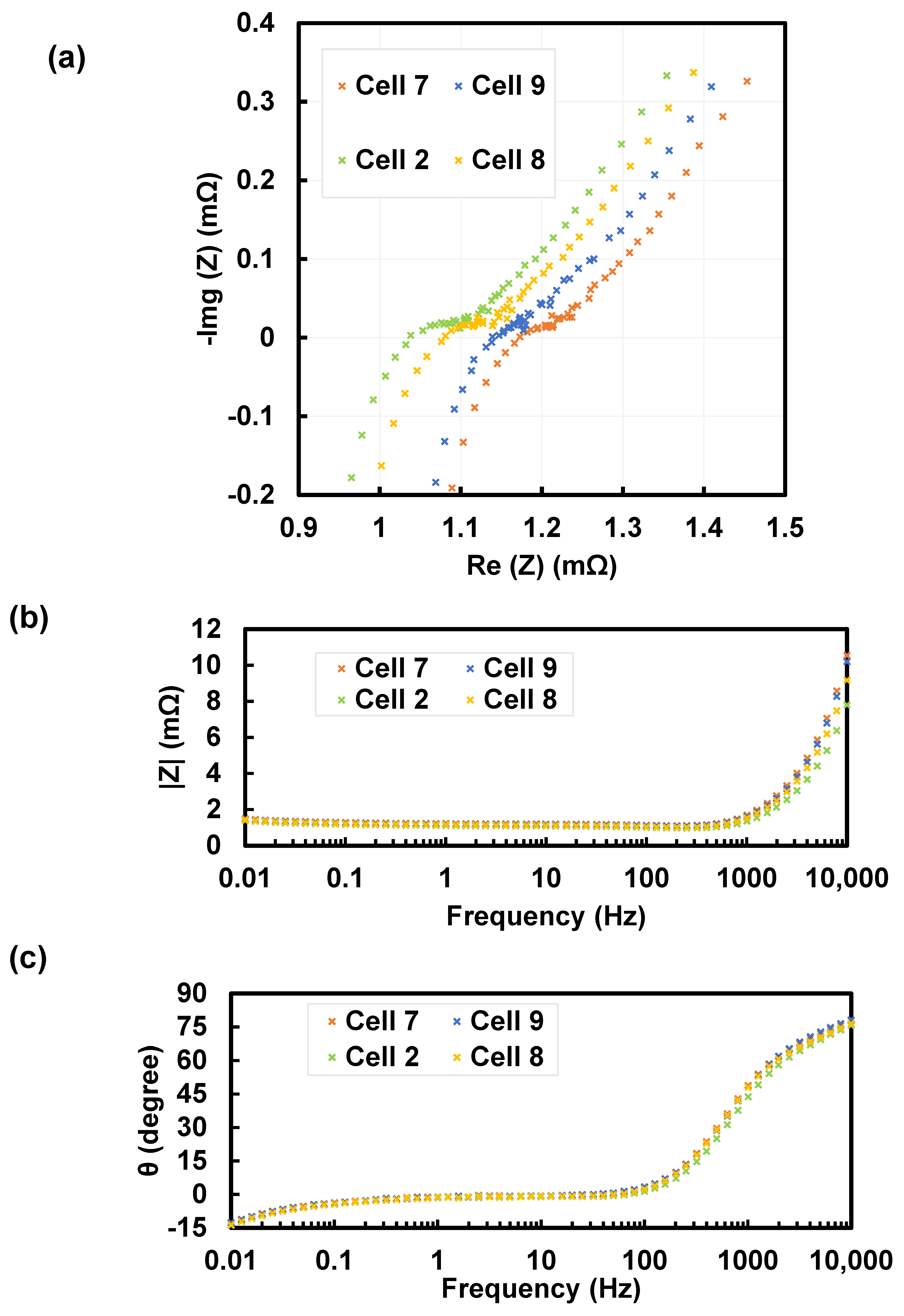
The Bode and Nyquist plots of other SOC and temperature conditions show similar trends. In general, higher SOC and temperature result in a smaller semi-circle on the Nyquist plot. The simple cell-to-cell variability comparison is presented in Appendix B. A preliminary quantitative inter-cell dispersion study based on ECM parameters is presented in Appendix C. The effective ohmic resistance R s exhibited relatively limited dispersion across the evaluated conditions, with CV values below 7%. In contrast, the relative dispersion of R c t increased markedly at 40 °C, where the fitted resistance became very small, suggesting that both inter-cell differences and relative fitting uncertainty may become more influential in resolving the weak charge-transfer feature. The diffusion-related parameters R w and T showed substantial dispersion and are therefore interpreted cautiously in inter-cell comparisons. Measurements at 12% SOC and 40 °C were available only for Cell 7 and Cell 9; this condition was excluded from the quantitative four-cell summary and is presented descriptively only. Because the cells were obtained from a disassembled EV battery pack and their prior operating histories and storage conditions were not independently controlled, these statistics describe observed inter-cell dispersion in the as-is condition rather than intrinsic manufacturing uniformity.

3.3. ECM Model Parameters and Sensitivity Study

Section 3.2 demonstrates strong agreement between battery EIS measurements and analytical solutions. As we can see from these figures, diffusion effects modeled with a generalized Warburg element closely approximate the experimental data. The fits are particularly accurate at high frequencies (10–50 Hz), with most data points aligning well with the fitted curves. Although some noise is present at mid-range frequencies (0.2–10 Hz), the curve still effectively represents the signals. It is important to note that the median value of the test data was used for fitting rather than the mean. This method is best used to account for slight variations in testing conditions across repeated experiments. According to robust statistics, the median provides a more reliable estimate of central tendency than the mean in such scenarios [64].
Table 5 summarizes the ECM parameters, and residuals of the fitting results relative to the test data, fitted by Bayesian optimization. EV cells were tested under five conditions: 12% SOC at 25 °C, 50% SOC at 25 °C, 100% SOC at 25 °C, 50% SOC at 40 °C, and 100% SOC at 40 °C. The solution resistance R s and charge-transfer resistance R c t decrease with increasing temperature. This phenomenon is consistent with common understanding, since resistivity typically decreases with increasing temperature due to enhanced ionic mobility in the electrolyte. The inductor L is independent of state of charge and temperature. The inductance is believed to be caused by the large amount of metal foil used in the battery. The constant phase element (CPE) shows minimal sensitivity to temperature and SOC variations within the tested range, which is similar to the literature findings [65]. Similarly, the inductive effects arising from the metal foils inside the pouch cell are also largely unaffected by temperature and SOC.
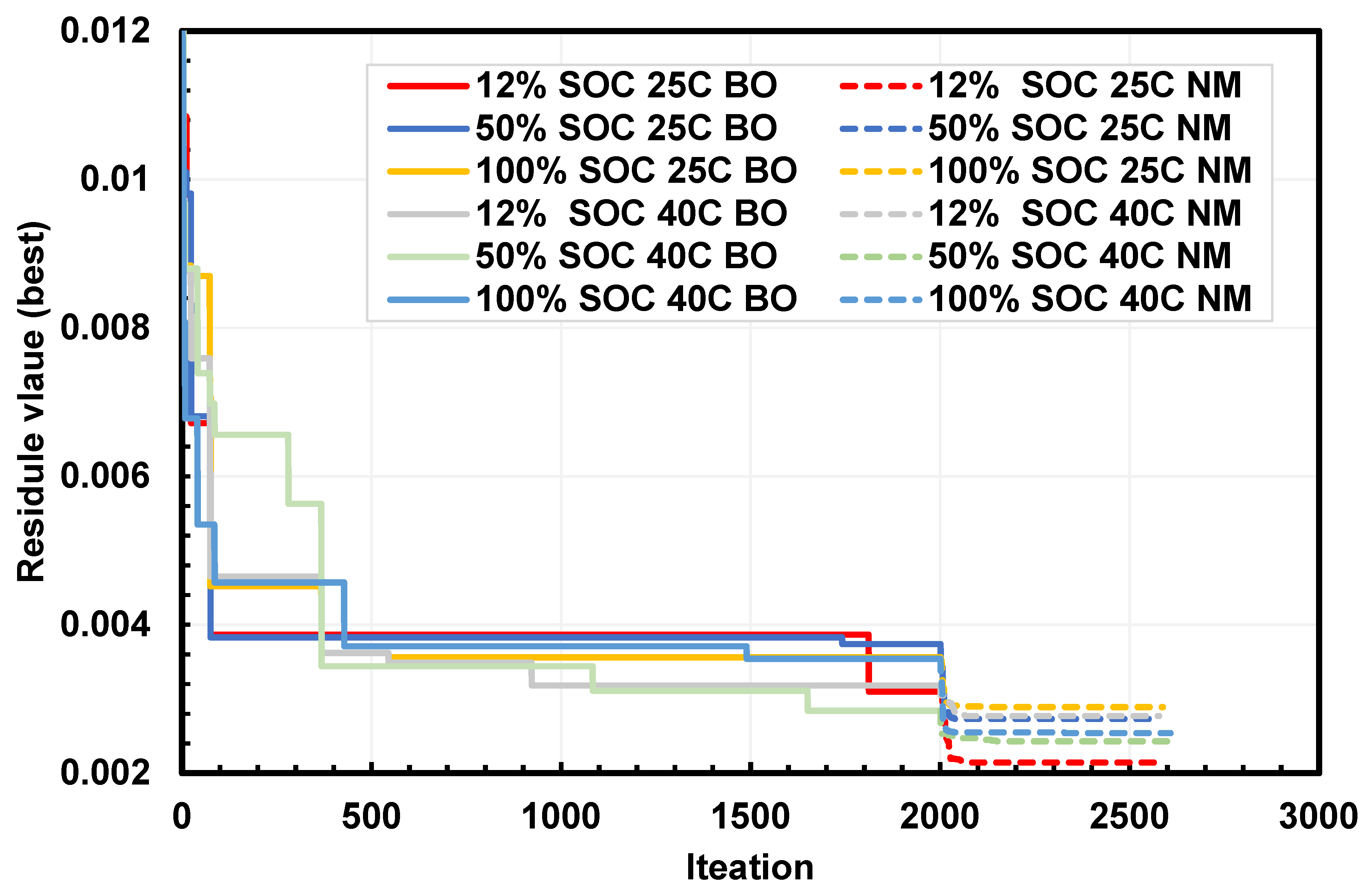
The residual value convergence histories showed similar qualitative behaviors, as shown in Figure 13. The solid line is the Bayesian optimization history, which represents the best value in the optimization history. It significantly reduces the residual value and provides a good starting point for local optimization to refine the parameters. The Nelder–Mead method, a local optimization technique, is indicated by the dash line. The global optimization was configured to run for 2000 iterations to generate a suitable starting point for local optimization, which allows the Nelder–Mead method to converge more efficiently.
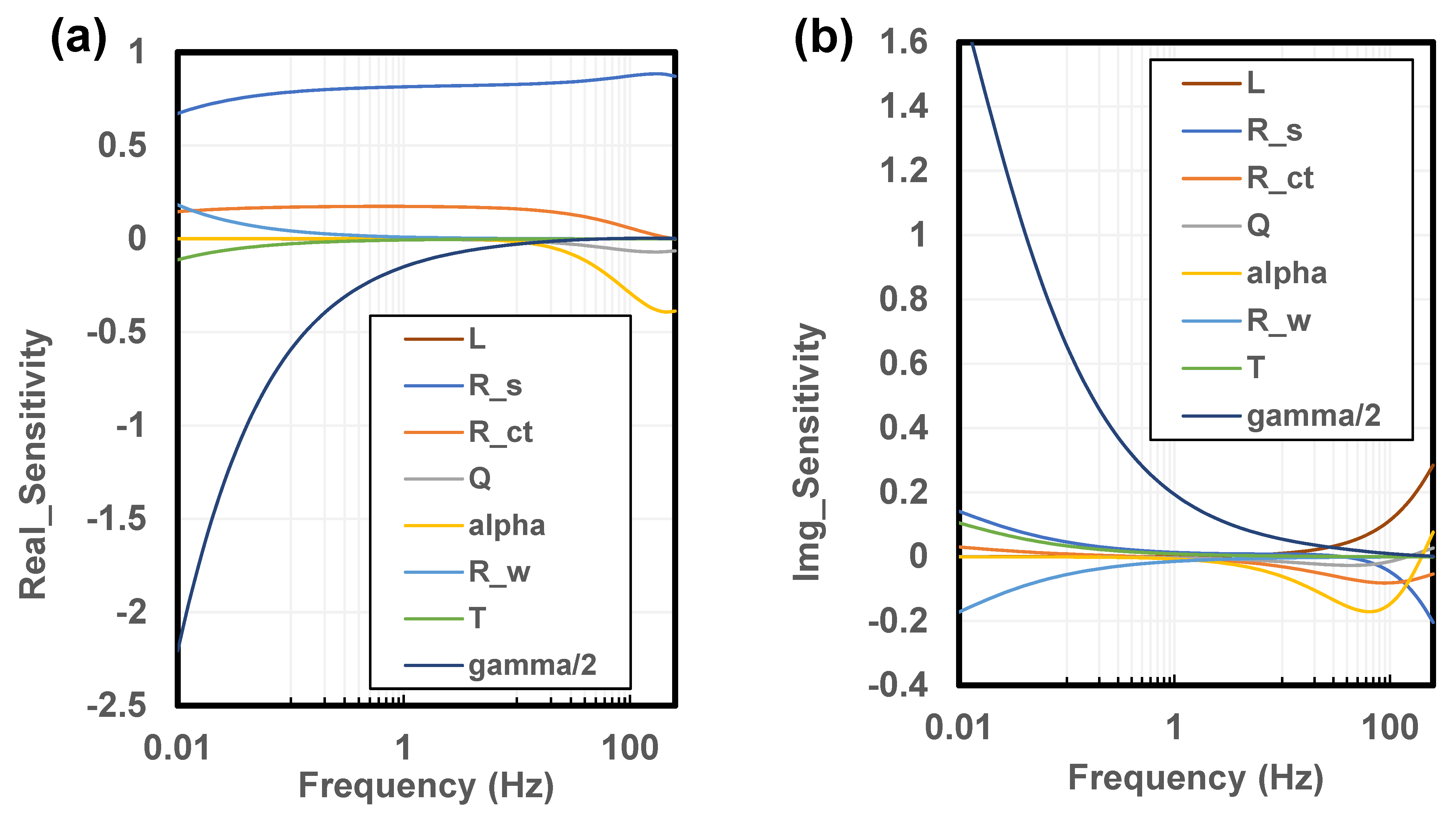
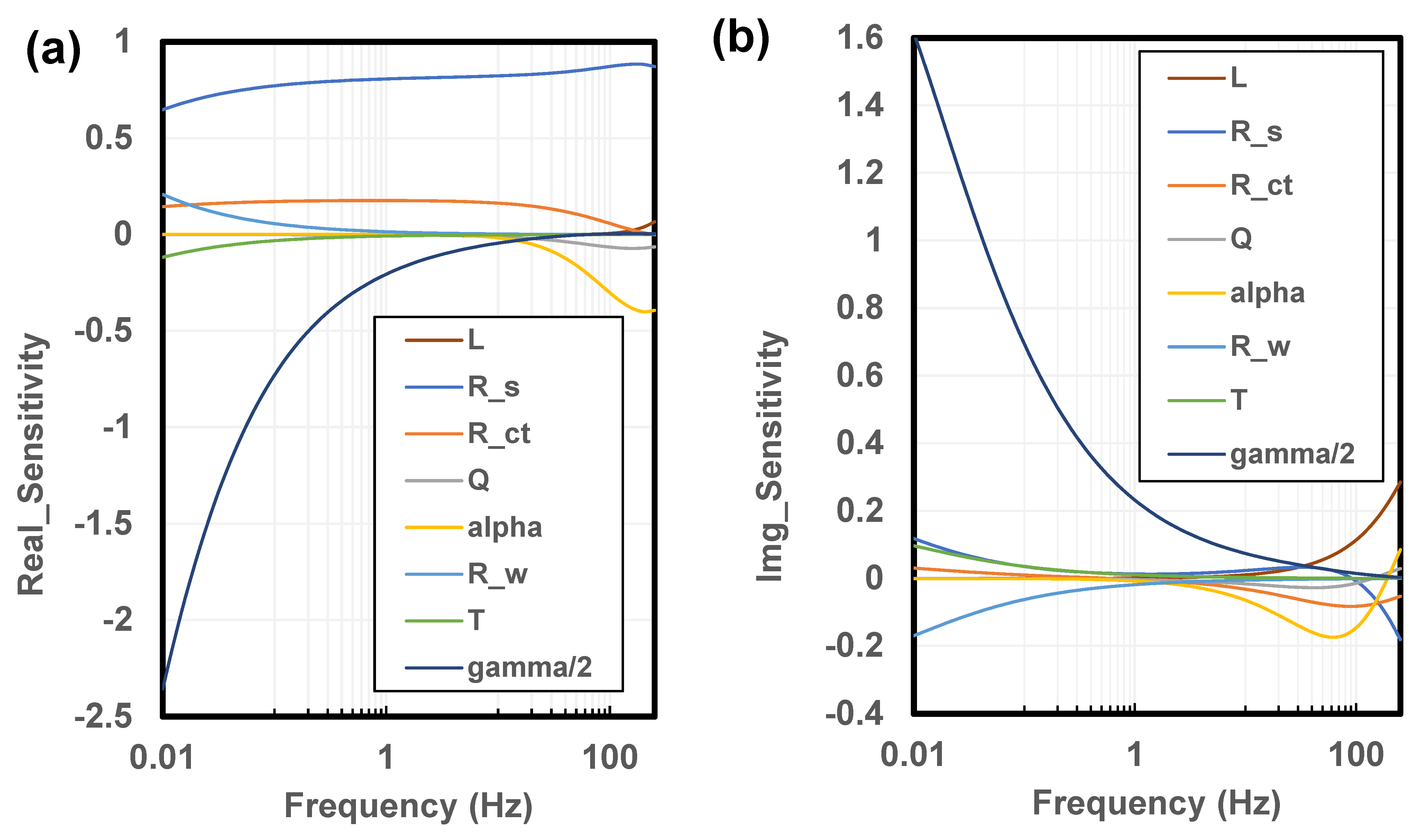
Figure 14 presents the typical frequency-dependent relative sensitivities of the model impedance to each circuit parameter, evaluated by:
S θ i Z = θ i Z Z θ i
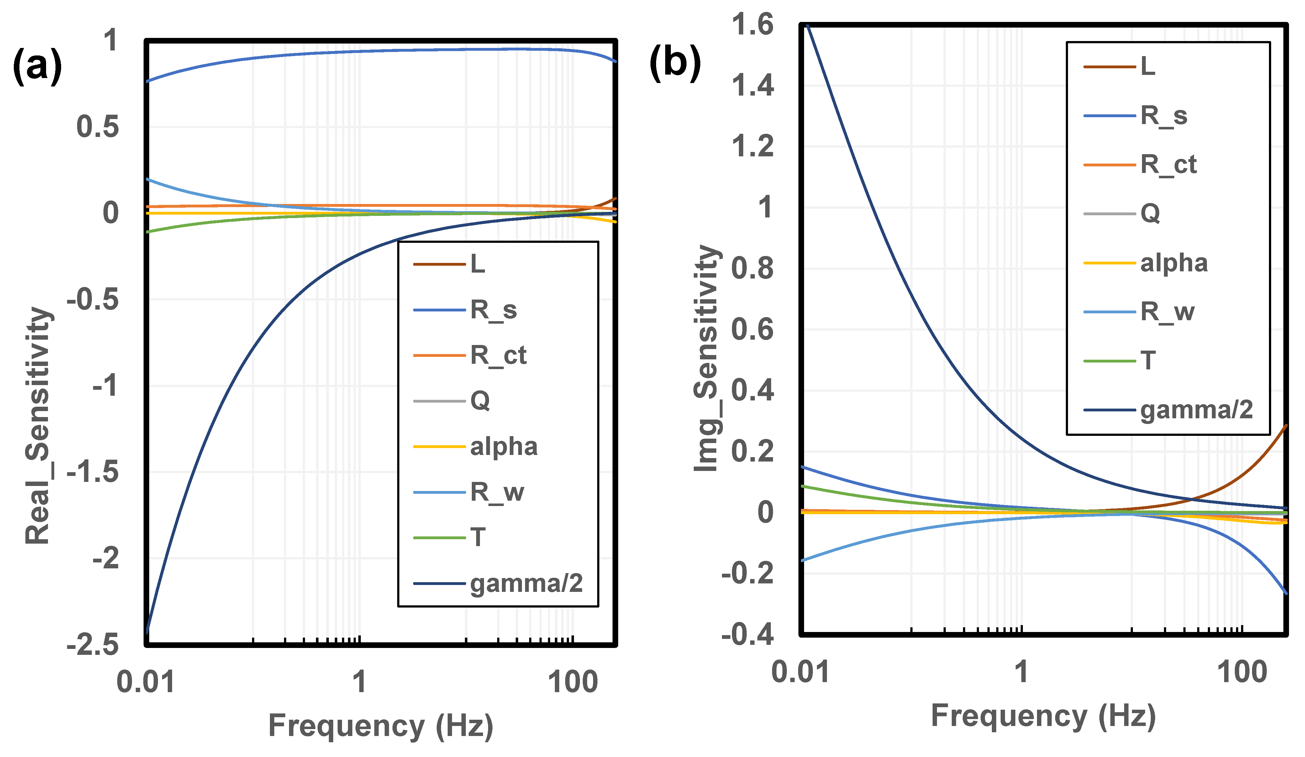
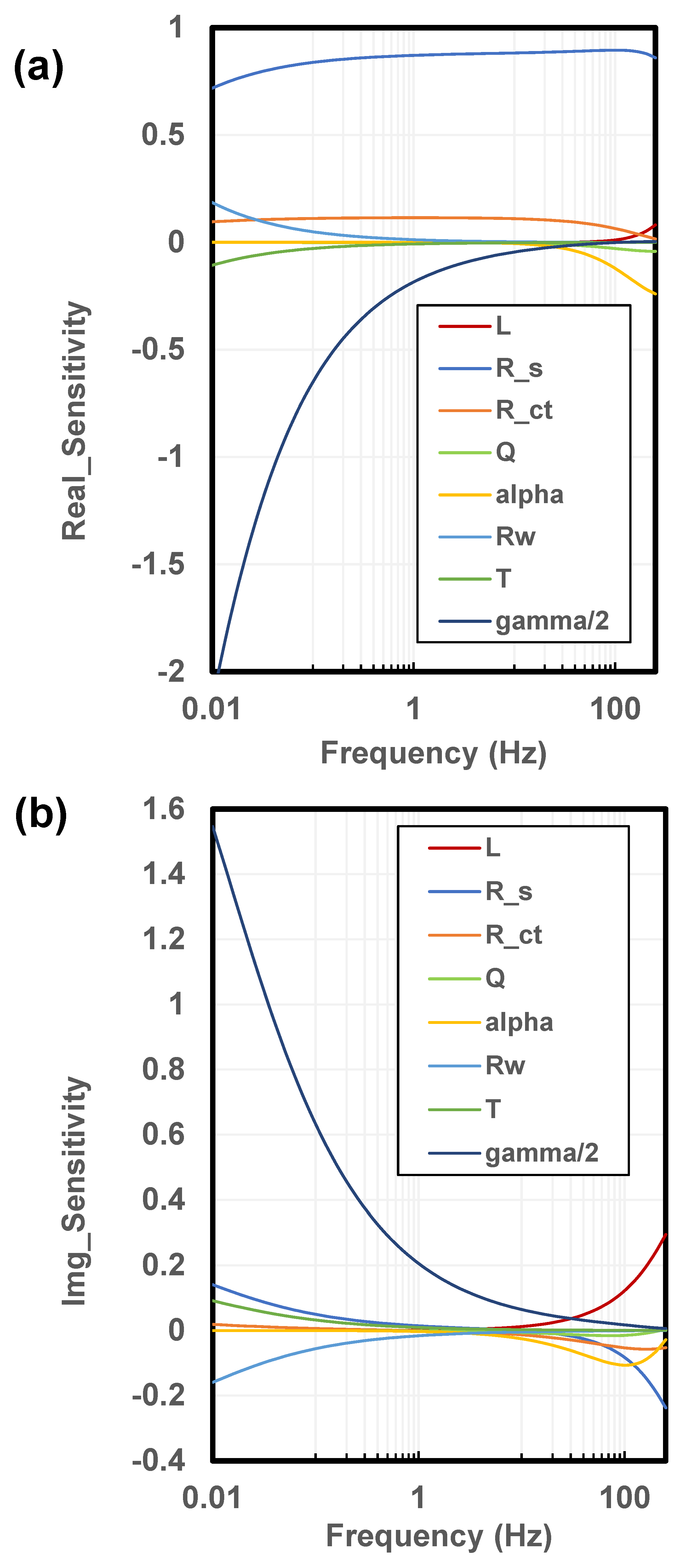
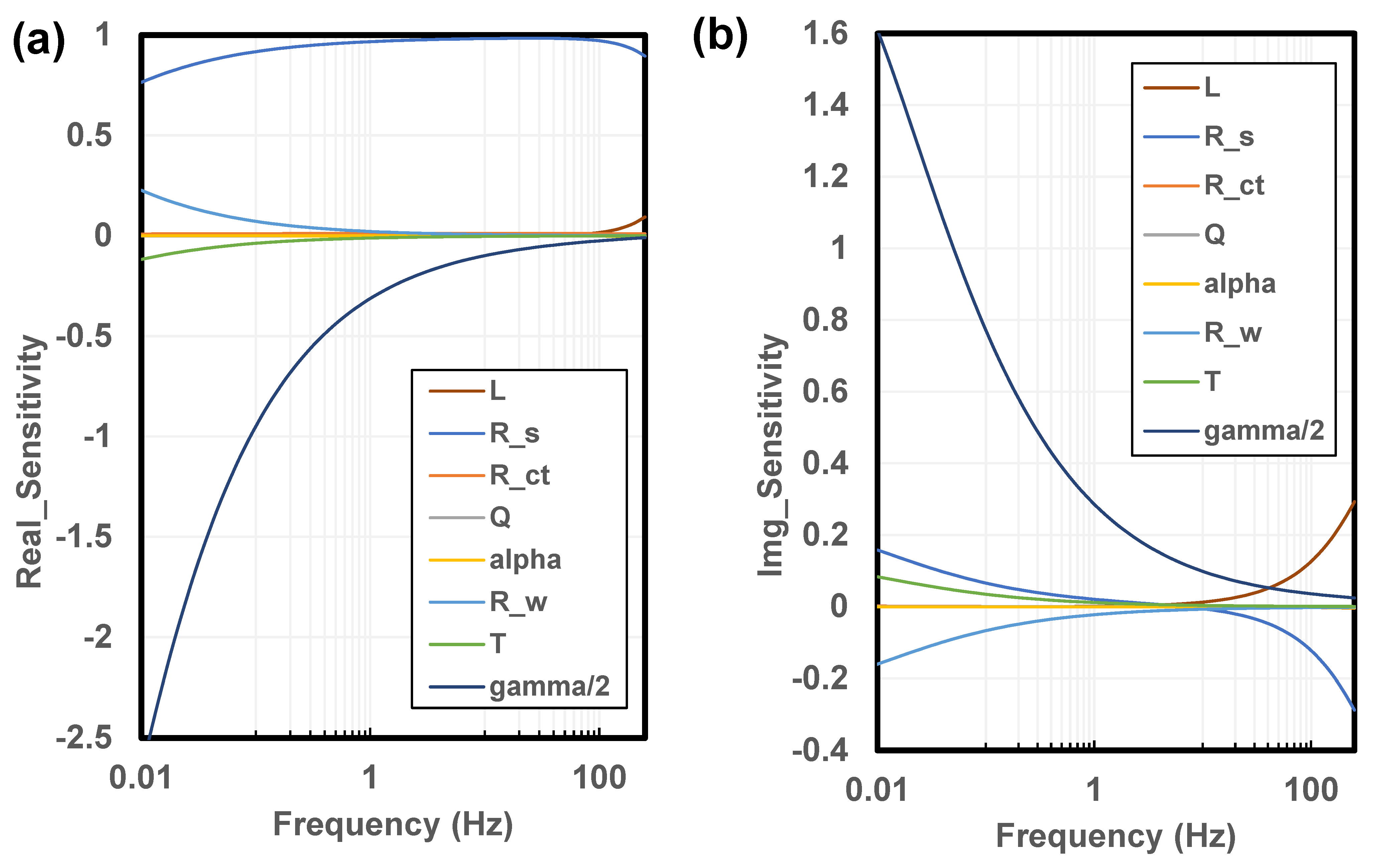
where S is the sensitivity function, θ i is the analyzed parameter, and Z is impedance. The function comes from [66]. The solution resistance exhibits a large and nearly frequency-independent sensitivity, indicating strong identifiability and dominant control of the real part of impedance. The charge-transfer resistance shows moderate sensitivity primarily in the mid-frequency range, consistent with its role in determining the diameter of the Nyquist semicircle. In contrast, CPE parameters display weaker and strongly frequency-dependent sensitivities, reflecting their influence on impedance dispersion. Diffusion-related parameters exhibit localized sensitivity at low frequencies, with the fractional diffusion exponent showing the largest sensitivity among all parameters. Sensitivity analyses were conducted for all investigated SOC and temperature conditions, and similar qualitative parameter-response trends were observed, as shown in Appendix E.

4. Discussion

In this paper, we studied the impedance spectrum and equivalent circuit model of a typical EV battery cell. A specialized battery fixture was designed to reduce contact resistance, enabling accurate EIS measurements for low-impedance batteries. A thermal chamber and battery cycler were used to measure EIS under varying temperatures and states of charge. An equivalent circuit model with well-defined physical meaning was chosen to interpret the EIS results. Bayesian optimization was used to fit the ECM parameters. It was observed that the CPE element and inductance are not significantly affected by changes in state of charge or temperature. The solution resistance and charge-transfer resistance both decrease as temperature increases. In this section, we focus on the significance of EIS findings in relation to experimental observations and model parameters.

4.1. EIS Experiment

The tested EV cells exhibit one of the lowest impedances reported for lithium-ion batteries in the EIS literature. It is interesting to see that some low impedance cell EIS data has no semicircles representing SEI [67,68,69,70,71], while others shows a second semi-circle attributed to the SEI [72,73]. In the present case, no distinct second semicircle attributable to an SEI-related contribution was resolved in the measured spectra. This may reflect either a comparatively small SEI contribution or overlap between SEI-related and charge-transfer responses within the measured frequency range. It is also seen that most of these low-impedance cells have a generalized Wartburg element, represented by a straight line with a non-45° angle [71,72]. This may be caused by the lack of testing data at very low frequencies. It is seen that a generalized Warburg element turns into a finite-space Warburg element when testing frequency reached the 0.001   H z range [69]. In our case, the lowest frequency is 0.01   H z .
Our results show a significant inductive effect on EIS data, as evidenced by the entire semicircle shifting toward the negative imaginary axis in the Nyquist plot. This behavior is likely caused by the large amount of metal foil used in the battery’s current collectors, which is substantially greater than in typical cylindrical batteries of smaller capacity. The observed high-frequency inductive response is attributed to the effective current pathway of the large-format pouch cell and the measurement connection, including contributions from current collectors, terminals, fixture contacts, and leads. This interpretation is further supported by observation that the inductance element in ECM model is largely unaffected by temperature variations.
Our EIS results show good repeatability and consistency, as seen in Figure 15. We found that to achieve accurate measurements for cells with impedance in the 1 mΩ range, the contact resistance between the battery terminals and test leads must be both small and stable from test to test. This is achieved by a custom-designed battery fixture that connects the terminals to the testing leads. The importance of the low-impedance battery fixture is demonstrated in Appendix D. EIS measurements were conducted on a precision resistor both with and without the fixture for comparison. Battery EIS data obtained using alligator clips are also presented. It is important to note that we did not use galvanostatic mode or high-current measurements. A potentiostatic perturbation amplitude of 1 mV was selected to limit disturbance to the low-impedance cell while maintaining a measurable response. The KK analysis supports the consistency of the spectra obtained under this condition. However, because a separate amplitude-dependence or harmonic distortion analysis was not performed, the present study does not independently establish the linear response range of the tested cell in the EIS theory. We do not find the potentiostatic mode has inferior accuracy compared to the galvanostatic mode for our equipment, contrary to the findings reported in the literature [74]. In theory, if current control is facilitated via a PID controller, the accuracy of the controller may also influence the precision of the measurement, which may offset many advantages associated with the current control mode. In fact, we observed that potentiostatic mode yielded enough accuracy for our GAMRY 5000P (Gamry Instruments, Inc., Warminster, PA, USA). Compared to previously reported EIS experiments, our experimental design did not require the application of high current to the system. This aspect is particularly important because one of the fundamental assumptions of EIS is that the system under investigation remains linear, stable, and time-invariant during the measurement. Applying high currents can lead to nonlinear responses, such as electrode polarization, heating effects, or electrochemical side reactions, which violate the linearity assumption and compromise the validity of the impedance data.
In addition, for the low-impedance cell investigated in this study, unstable terminal contact can introduce a contribution comparable to the measured cell impedance. The custom fixture was therefore designed to provide a stable, low-resistance connection for four-terminal EIS measurements.
The high contact resistance caused by a loose connection also introduces an inductance effect that will pollute the response signal and cause repeatability issues.
This is particularly important at low frequencies, where measurement artifacts tend to be more pronounced. Many conventional EIS test setups exhibit relatively high contact and lead resistances, which can obscure subtle electrochemical features and reduce the fidelity of equivalent-circuit modeling. Therefore, our low-resistance configuration plays a critical role in enhancing the quality and reliability of the EIS data. Alligator clips often introduce significant errors in EIS measurements due to unstable contact resistance, as well as parasitic inductance and capacitance. They are also susceptible to electromagnetic interference. These issues can distort system responses, leading to inaccurate impedance spectra and poor reproducibility. For accurate EIS measurements, it is recommended to use a battery holder with low contact resistance and a stable, screw-fastened connection between the test leads and the battery.
In addition to the measurement accuracy, another challenge of EIS measurement is the voltage range. High-voltage EIS measurement on the module and pack level is necessary to develop ECM models for EVs. The current electrochemical workstation normally has a DC voltage range of less than 10   V , which makes the measurement of battery modules (e.g., 30   V ) infeasible. Future development should focus on extending the capabilities of existing equipment or developing new systems to enable EIS measurements on multi-cell battery modules.

4.2. EIS Model

The selected ECM was designed to represent the principal features resolved in the measured spectra: an effective series inductive contribution at high frequency, an ohmic contribution, a depressed interfacial semicircle, and a non-ideal diffusion-related low-frequency response. The CPE and generalized Warburg terms should therefore be interpreted as effective elements representing distributed interfacial and transport behavior rather than direct measurements of individual microscopic properties. The inductive contribution is retained because it is non-negligible for the milliohm-scale response of the tested pouch cell and its measurement pathway.
The extracted ECM parameters provide potential diagnostic features for future battery management applications. In the present results, both the solution resistance R s and charge-transfer resistance R c t exhibit clear temperature dependence across the investigated SOC conditions, with lower values generally observed at elevated temperature. This behavior is relevant to battery management because impedance-based diagnostic features must be interpreted with temperature compensation rather than treated as temperature-independent indicators. In a practical BMS framework, R s may serve as an effective descriptor of changes in the overall ohmic response, while R c t may provide information related to interfacial kinetic behavior. When calibrated over broader SOC, temperature, aging, and operating-condition ranges, these parameters could potentially contribute to SOC/SOH estimation and abnormal-condition detection.
It is worth emphasizing that the inter-cell discrepancy must be considered in the design of future battery management applications. As shown in Appendix B, noticeable differences in the EIS responses were observed among cells within the same battery module. As shown in Figure 7, Figure 8, Figure 9, Figure 10, Figure 11 and Figure 12, the repeatability tests yielded very small standard deviations. Therefore, the discrepancies observed in Appendix B are attributed to intrinsic cell-to-cell variability rather than measurement uncertainty. Appendix C quantitatively compares the cell-to-cell discrepancy with the fitted ECM models. For example, the coefficient of variation for R c t increased substantially at 40 °C, as shown in Appendix C. Therefore, establishing R c t as a quantitatively standalone diagnostic parameter should be carried out on each cell, not taking average values. Future research also requires validation using a larger number of cells, controlled aging histories, and a more comprehensive uncertainty analysis for developing the EIS-based BMS. In addition, the selected ECM provides an effective parameterized representation for future investigations of electrode–electrolyte interfacial phenomena, particularly through the evolution of R c t , CPE-related parameters, and diffusion-related terms. These parameters should be interpreted as lumped descriptors of the impedance response rather than unique measurements of individual microscopic processes.
Notice that the EIS curve in the Nyquist plot has a negative slope when frequency goes higher than 499 Hz, as seen in Figure 6. Current ECM models are not suitable to model the battery high-frequency behavior (251 Hz to 10 kHz), where the cell largely behaves like an inductor.
The summary of tests and ECM fittings results with different SOC and temperature are presented in Figure 15.

4.3. Optimization

The BO-NM procedure was used in this study as a global-to-local parameter-identification strategy for the selected ECM. Bayesian optimization was employed to explore the bounded parameter space and identify a suitable candidate solution, which was subsequently refined using the Nelder–Mead method. Future work should focus on the method comparison between BO-NM method with other mainstream EIS fitting methods.

5. Conclusions

The major contributions of this paper include the following: (1) A specially designed battery fixture that enables accurate EIS measurements for low-impedance cells in the 1 mΩ range. (2) Bayesian optimization is applied to fit ECM parameters based on EIS data. (3) We present the impedance spectrum and corresponding ECMs for typical Li-ion battery cells used in EVs, which supports the development of future onboard EIS systems for battery diagnostics. (4) We find that charge-transfer resistance, solution resistance, and diffusion time are sensitive to both temperature and SOC, offering valuable insights for electrochemical battery testing.
The specially designed fixture is critical for minimizing contact resistance during EIS measurements. An adaptable four-terminal fixture architecture was developed to provide stable terminal contact, separated current-carrying and voltage-sensing pathways, and a measurement configuration compatible with open/short calibration. Because this design addresses the practical connection interface between the cell and the measurement system rather than relying solely on instrument-side improvements, it offers a potentially transferable engineering solution for low-impedance EIS measurements using systems capable of Kelvin sensing and appropriate calibration. Our results show that the EIS measurement for a battery with 1 mΩ internal resistance can be performed without relying solely on high-current excitation or instrument-side improvements.
The selected ECM represents the principal features of the measured spectra through an effective series inductance, an ohmic resistance, a CPE/charge-transfer branch, and a generalized diffusion-related element. The inductive-response segment retained in the fitting was used to identify the effective series inductance associated with the low-impedance cell measurement pathway and was not interpreted as an electrode–electrolyte interfacial process. Across the investigated SOC conditions, the fitted ohmic resistance and charge-transfer resistance exhibited clear temperature dependence and generally decreased at 40 °C relative to 25 °C. These observations indicate that such parameters may serve as temperature-compensated impedance features in future battery diagnostic and management applications, although their suitability for quantitative diagnostic applications depends on parameter identifiability, inter-cell variability, and validation over broader operating conditions.
The BO-NM procedure was applied as a parameter-identification approach for the selected ECM. A broader comparison with additional fitting methods remains important for future work. The method of using custom-designed fixtures reduces the error in the EIS measurement. The effective ECM framework provides a basis for future studies of aging, fault-related behavior, and electrode–electrolyte interfacial and transport phenomena in commercial EV cells. Further validation using additional cells with controlled aging histories, quantitative repeatability metrics, broader operating conditions, and alternative cell formats and chemistry are required before extending this approach to onboard or module-level applications.


6. Further Work

Future work should focus on building this ECM into a multi-physic finite element analysis for battery safety study. Future ECM should also include inductance properties on the high-frequency side, where the line in the Nyquist plot is extended to the lower right. The physical explanation of high-frequency battery behavior (251 Hz to 10 kHz) needs to be investigated. Higher temperature, including the battery thermal runaway temperature, should be studied for its EIS diagram. Non-classical Warburg diffusion theory should be investigated to explain the physical meaning of a low-frequency slope greater than 45° in the low-frequency region of the Nyquist plot. The BO-NM method needs to be quantified for its effectiveness against other EIS fitting methods.

Author Contributions

Conceptualization, M.R.A., V.C., C.-D.K. and L.W.; Methodology, S.W., M.R.A., V.C., C.-D.K. and L.W.; Software, S.W., C.-D.K. and L.W.; Validation, S.W., M.R.A., V.C. and L.W.; Formal analysis, S.W., M.R.A., V.C. and L.W.; Investigation, S.W., M.R.A., V.C., C.-D.K. and L.W.; Resources, S.W., M.R.A., V.C., C.-D.K. and L.W.; Data curation, S.W., M.R.A., V.C. and L.W.; Writing—original draft, S.W., M.R.A. and L.W.; Writing—review & editing, S.W., V.C. and L.W.; Visualization, S.W., M.R.A., V.C. and L.W.; Supervision, M.R.A., V.C., C.-D.K. and L.W.; Project administration, M.R.A., V.C., C.-D.K. and L.W.; Funding acquisition, V.C., C.-D.K. and L.W. All authors have read and agreed to the published version of the manuscript.

Funding

This research was in part funded by American Chemical Council Life Cycle Analysis Program.

Data Availability Statement

Data is contained within this article.

Acknowledgments

This work was in part supported by the American Chemical Council Life Cycle Analysis Program under the leadership of Muys Wesley and William Thomas Hollowell. The authors gratefully acknowledge their support and guidance. The authors gratefully acknowledge Teng Long (ORCID: 0000-0001-9573-5816) for his essential technical guidance and substantial contributions to the development, implementation, and application of the Bayesian optimization and Nelder–Mead algorithms for EIS parameter identification. His expertise and instruction were very important in establishing the optimization framework used in this study.

Conflicts of Interest

Authors Masoud Rostami Angas and Vidyu Challa were employed by the company Reliability Engineering Services, Ansys Part of Synopsys. The remaining authors declare that the research was conducted in the absence of any commercial or financial relationships that could be construed as potential conflicts of interest.

Appendix A. The KK Validity Results

The KK validity result for “Cell 7” at a different state of charge and temperature is summarized in Figure A1, Figure A2, Figure A3, Figure A4 and Figure A5. In total, 50 parallel RC networks were used in the KK fit.
Figure A1. Linear Kramers–Kronig validation of experimental EIS at 50% SOC and 25 °C. Nyquist plot (a) and frequency-dependent relative errors of real and imaginary impedance (b). Overall relative error = 0.15%.
Coatings 16 00930 g0a1
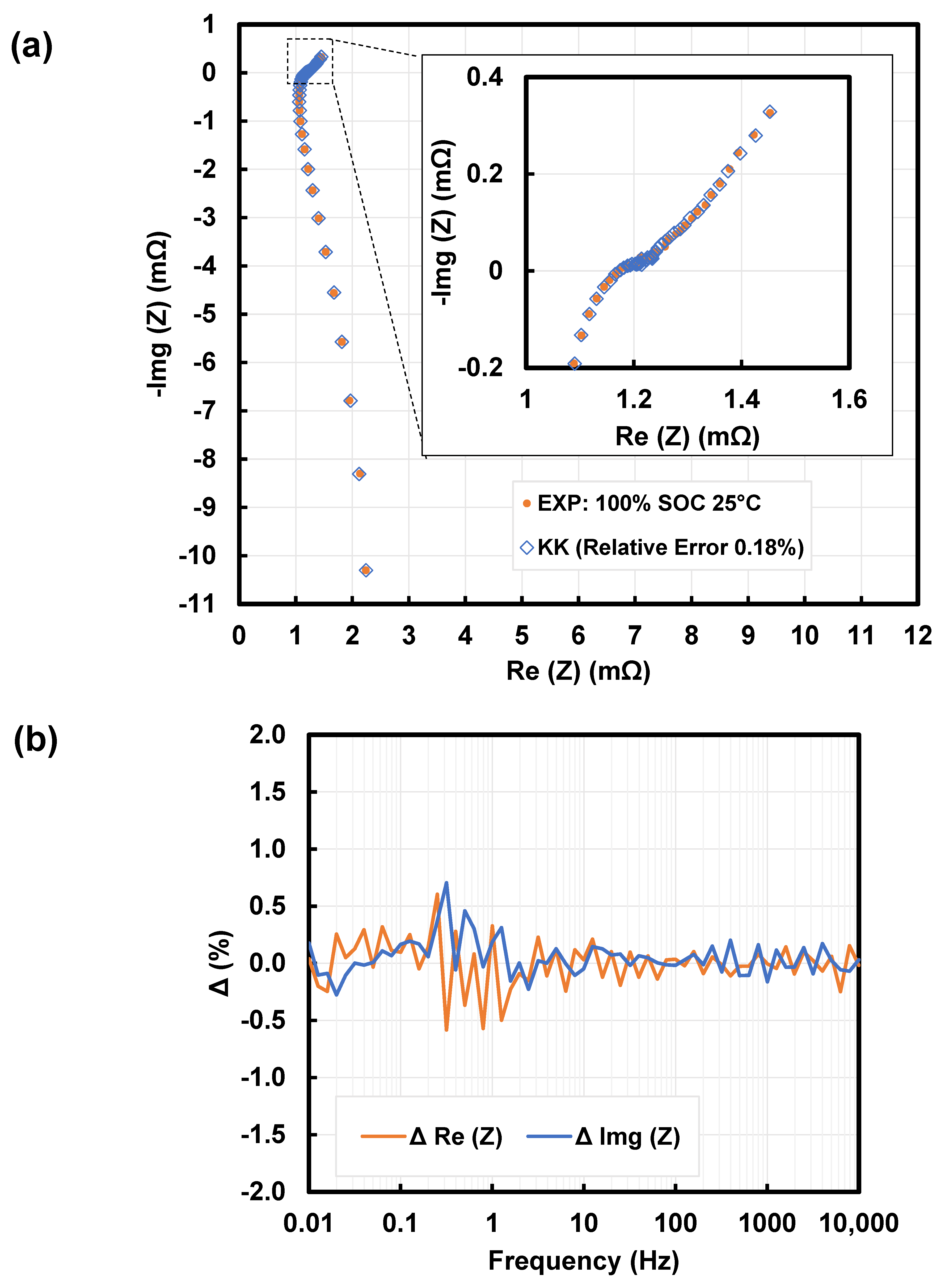
Figure A2. Linear Kramers–Kronig validation of experimental EIS at 100% SOC and 25 °C. Nyquist plot (a) and frequency-dependent relative errors of real and imaginary impedance (b). Overall relative error = 0.18%.
Coatings 16 00930 g0a2
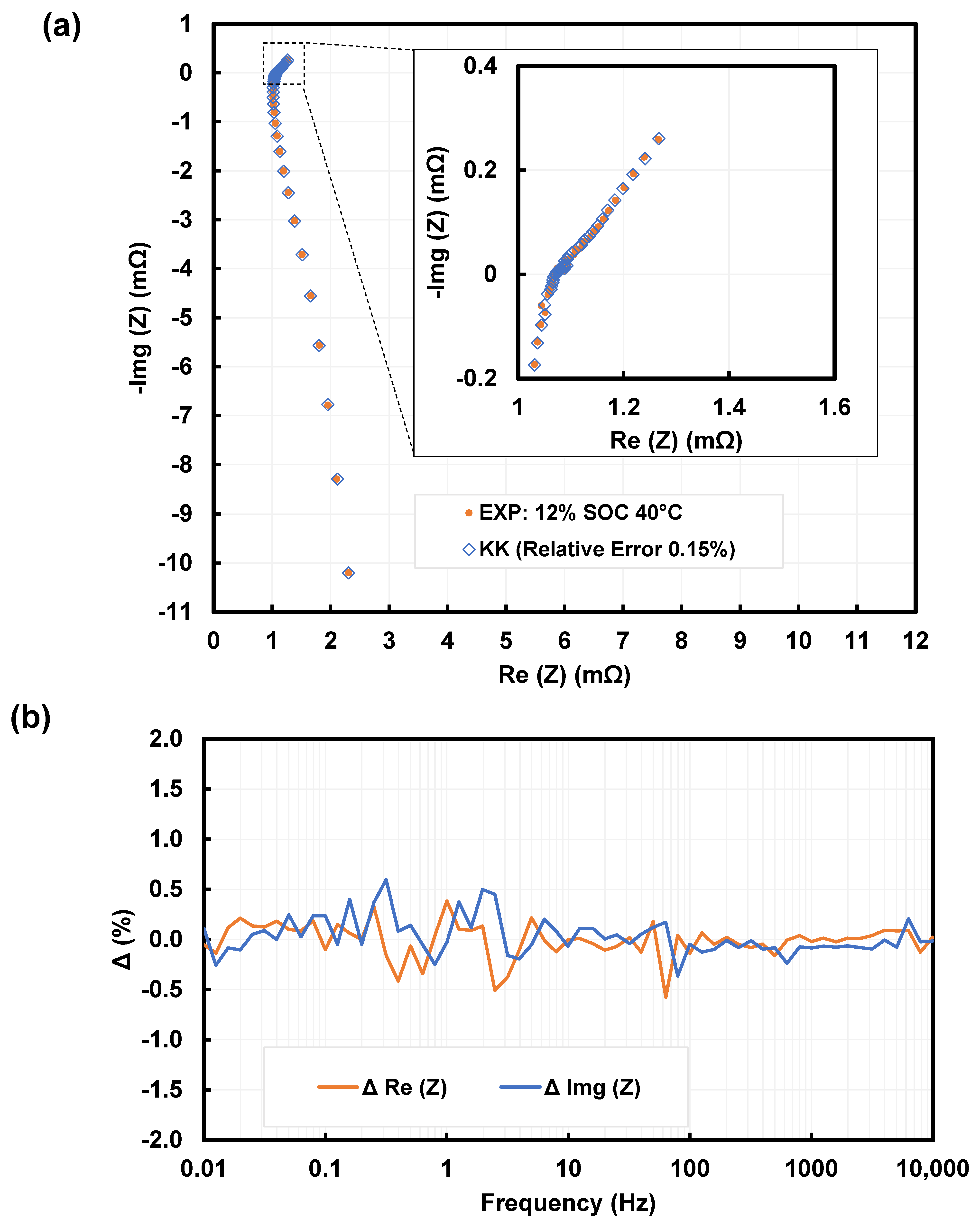
Figure A3. Linear Kramers–Kronig validation of experimental EIS at 12% SOC and 40 °C. Nyquist plot (a) and frequency-dependent relative errors of real and imaginary impedance (b). Overall relative error = 0.15%.
Coatings 16 00930 g0a3
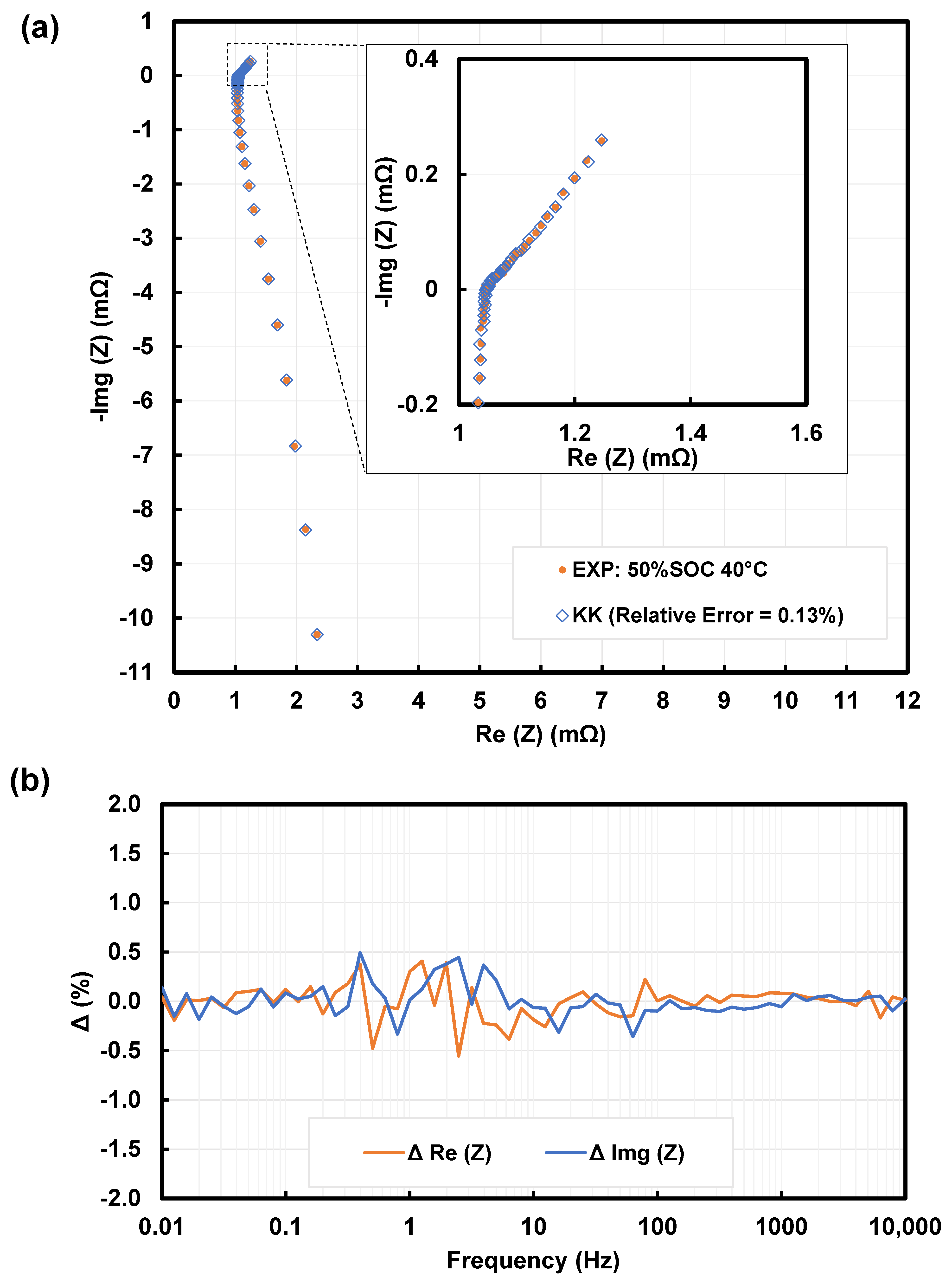
Figure A4. Linear Kramers–Kronig validation of experimental EIS at 50% SOC and 40 °C. Nyquist plot (a) and frequency-dependent relative errors of real and imaginary impedance (b). Overall relative error = 0.13%.
Coatings 16 00930 g0a4
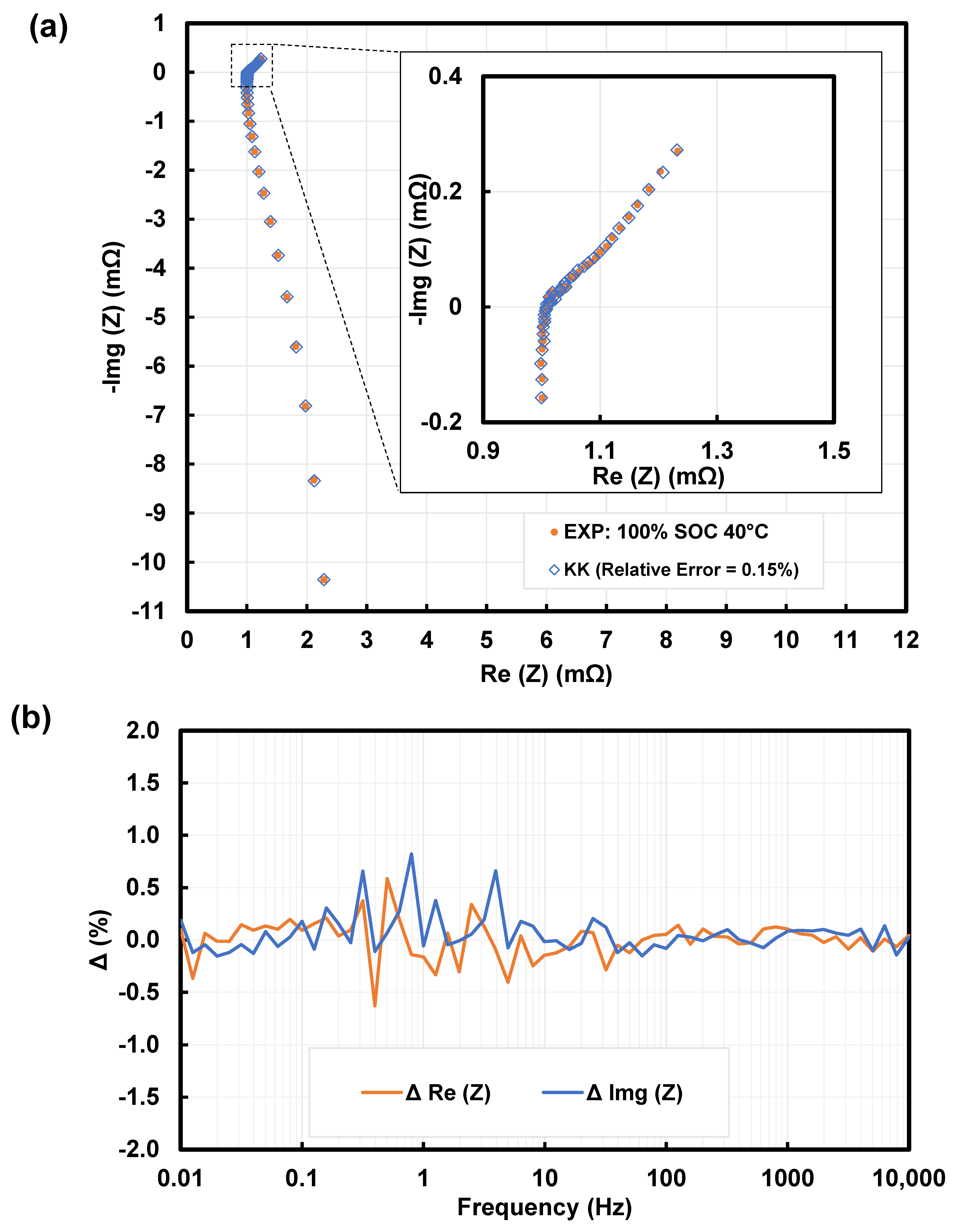
Figure A5. Linear Kramers–Kronig validation of experimental EIS at 100% SOC and 40 °C. Nyquist plot (a) and frequency-dependent relative errors of real and imaginary impedance (b). Overall relative error = 0.15%.
Coatings 16 00930 g0a5

Appendix B. The Discrepancy Among Different Cells

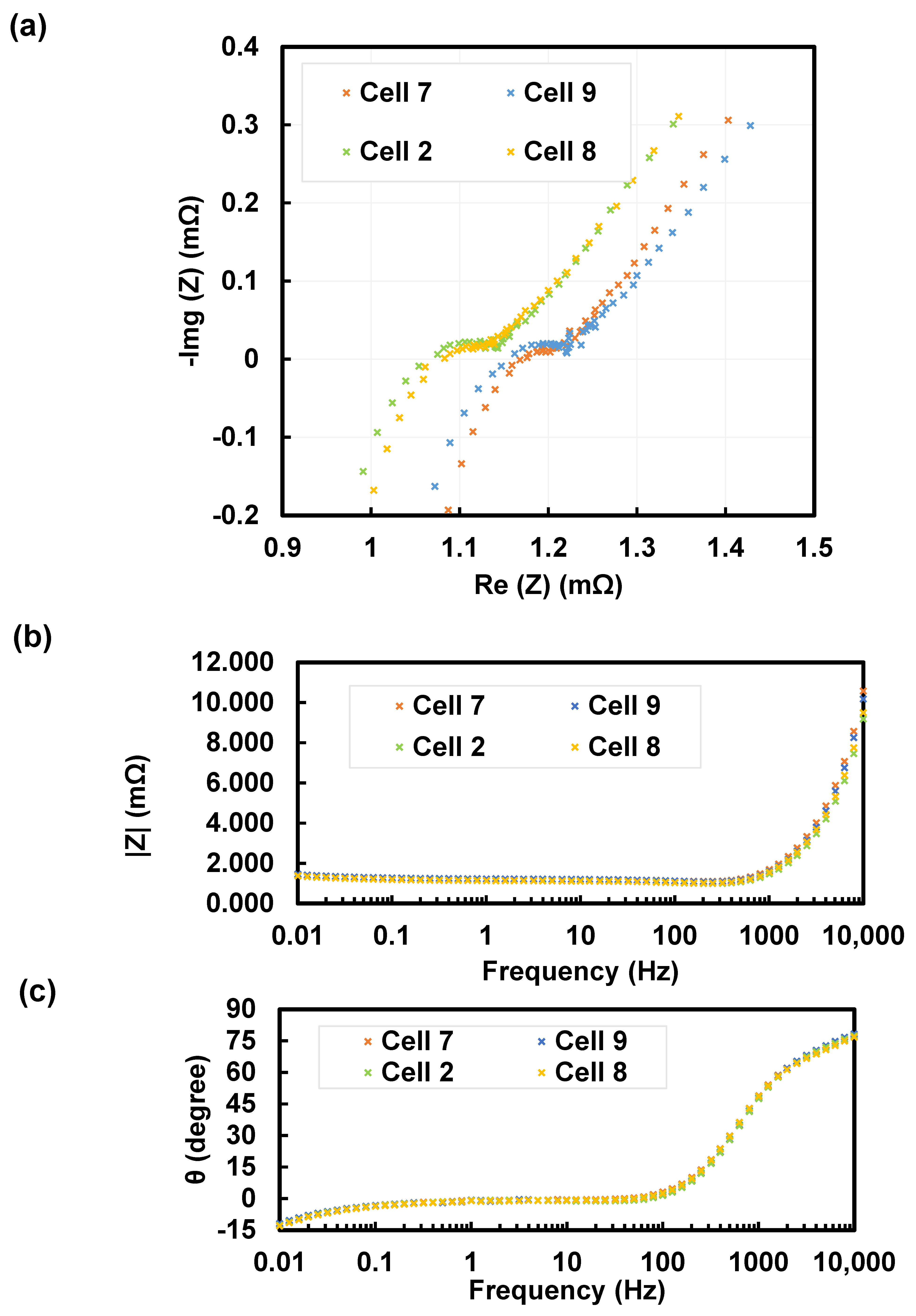
This appendix summarizes the differences between different cells within the same battery module. Four cells were disassembled from the same battery module and are tested under identical conditions. For each cell, multiple tests were conducted following the same procedures described in previous sections. The results showed excellent repeatability. Therefore, for simplicity and clarity, only one representative test result per cell under each test condition is presented. The results presented in the preceding sections were obtained from tests conducted on Cell 7.
Figure A6. Nyquist plot (a) and Bode plot (b,c) of 12% SOC, 25 °C.
Coatings 16 00930 g0a6
Figure A7. Nyquist plot (a) and Bode plot (b,c) of 12% SOC, 40 °C.
Coatings 16 00930 g0a7
Figure A8. Nyquist plot (a) and Bode plot (b,c) of 50% SOC, 25 °C.
Coatings 16 00930 g0a8
Figure A9. Nyquist plot (a) and Bode plot (b,c) of 50% SOC, 40 °C.
Coatings 16 00930 g0a9
Figure A10. Nyquist plot (a) and Bode plot (b,c) of 100% SOC, 25 °C.
Coatings 16 00930 g0a10
Figure A11. Nyquist plot (a) and Bode plot (b,c) of 100% SOC, 40 °C.
Coatings 16 00930 g0a11

Appendix C. The Preliminary Cell Discrepancy Evaluation with ECM

The multi-cell ECM fitting results are presented here as a rough method to evaluate the cell-to-cell discrepancy. The average ECM parameter of four cells (“Cell 2”, “Cell 7”, “Cell 8” and “Cell 9”) are presented in Table A1.
x ¯ = 1 N i = 1 N x i
where x i stands for the ECM parameter of i -th cell, x ¯ represents the mean value of ECM parameter, and N = 4 stands for the four tested cells. Standard deviation σ of the ECM parameter is shown in Table A2.
σ = 1 N i = 1 N x i x ¯ 2
The coefficient of variation C V is shown in Table A3.
C V = σ x ¯ × 100 %
Table A1. Mean value of 4 cells’ ECM parameter.
ECM Parameter Fit by BO-NM (Unit)12% SOC 25 °C50% SOC 25 °C100% SOC 25 °C50% SOC 40 °C100% SOC 40 °C
L ( H ) 1.8625 × 10⁻⁷
R s (Ω)9.5232 × 10−49.3010 × 10−49.2724 × 10−49.4148 × 10−49.3535 × 10⁻⁴
R c t (Ω)4.2985 × 10−42.4859 × 10−42.2607 × 10−43.3753 × 10−51.5879 × 10⁻⁵
Q ( Ω 1 s α ) 26.635
α 0.72491
R w (Ω)49.46836.05624.02541.73115.695
T ( s ) 1.1493 × 1094.3384 × 1097.7941 × 1091.1586 × 10112.6630 × 1010
γ / 2 0.663000.611130.563870.543030.51249
Table A2. Standard deviation of 4 cells’ ECM parameter.
ECM Parameter Fit by BO-NM (Unit)12% SOC 25 °C50% SOC 25 °C100% SOC 25 °C50% SOC 40 °C100% SOC 40 °C
L ( H ) 2.0907 × 10⁻⁸
R s (Ω)6.3373 × 10−55.6942 × 10−56.1331 × 10−53.7002 × 10−54.3408 × 10⁻⁵
R c t (Ω)7.8502 × 10−52.2761 × 10−52.2716 × 10−52.6587 × 10−51.5912 × 10⁻⁵
Q ( Ω 1 s α ) 2.7692
α 0.025195
R w (Ω)80.96141.98028.01656.85112.114
T ( s ) 1.9927 × 1097.1293 × 1091.2752 × 10102.1779 × 10113.0095 × 1010
γ / 2 1.8371 × 10−26.8795 × 10−35.8654 × 10−37.9042 × 10−37.2182 × 10⁻³
Table A3. Coefficient of variation of 4 cells’ ECM parameter.
ECM Parameter Fit by BO-NM (Unit)12% SOC 25 °C50% SOC 25 °C100% SOC 25 °C50% SOC 40 °C100% SOC 40 °C
L ( H ) 11.2252%
R s (Ω)6.6546%6.1222%6.6143%3.9302%4.6409%
R c t (Ω)18.2627%9.1560%10.0482%78.7688%100.2091%
Q ( Ω 1 s α ) 10.3930%
α 3.4756%
R w (Ω)163.6657%116.4303%116.6143%136.2318%77.1839%
T ( s ) 173.3818%164.3303%163.6109%187.9720%113.0115%
γ / 2 2.7710%1.1257%1.0402%1.4556%1.4085%

Appendix D. The Influence of Testing Lead Contact Resistance on EIS

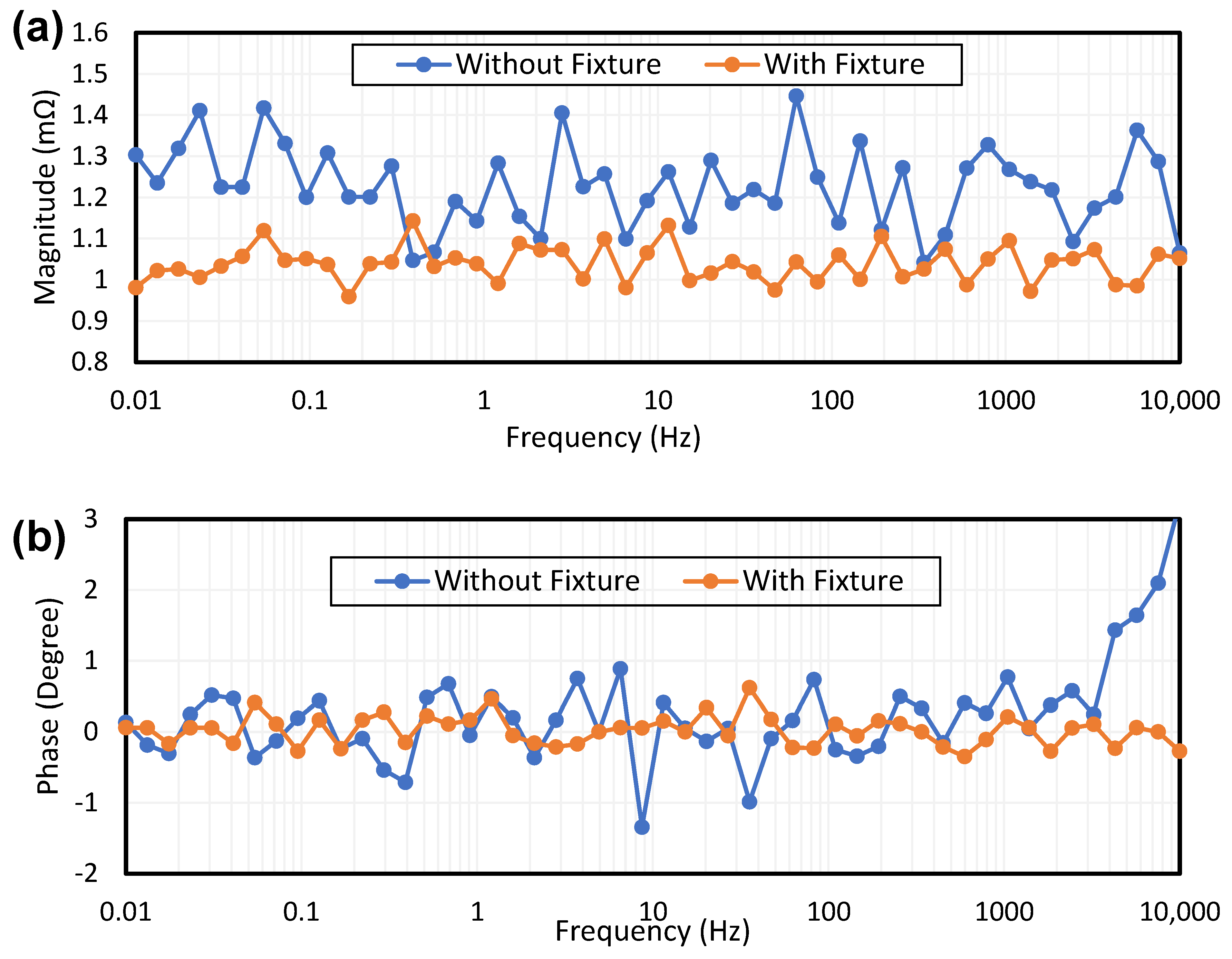
Reducing the contact impedance between battery and analyzer leads is critical for accurate EIS measurement in the low-impedance range. To demonstrate this point, a precision low-value resistor (1 mΩ, ±1% tolerance) was characterized using the same Gamry 5000P analyzer and the identical measurement configuration in four-electrode potentiostatic mode, as used for the battery tests. Measurements were performed both with and without the custom fixture to isolate the effect of the connection method. Across five repeated measurements, the custom fixture reduced the standard deviation of the measured real impedance by approximately 57% and reduced the absolute measurement error from 0.25 mΩ (alligator clips) to below 0.05 mΩ, confirming that the fixture enables sub-milliohm resolution under the same analyzer settings. These results demonstrate that the low-impedance fixture is essential for achieving accurate and repeatable milliohm-level EIS measurements.
Figure A12. Nyquist plot for precision resistor tested with and without fixture (a) Magnitude error (b) Phase angle error.
Coatings 16 00930 g0a12
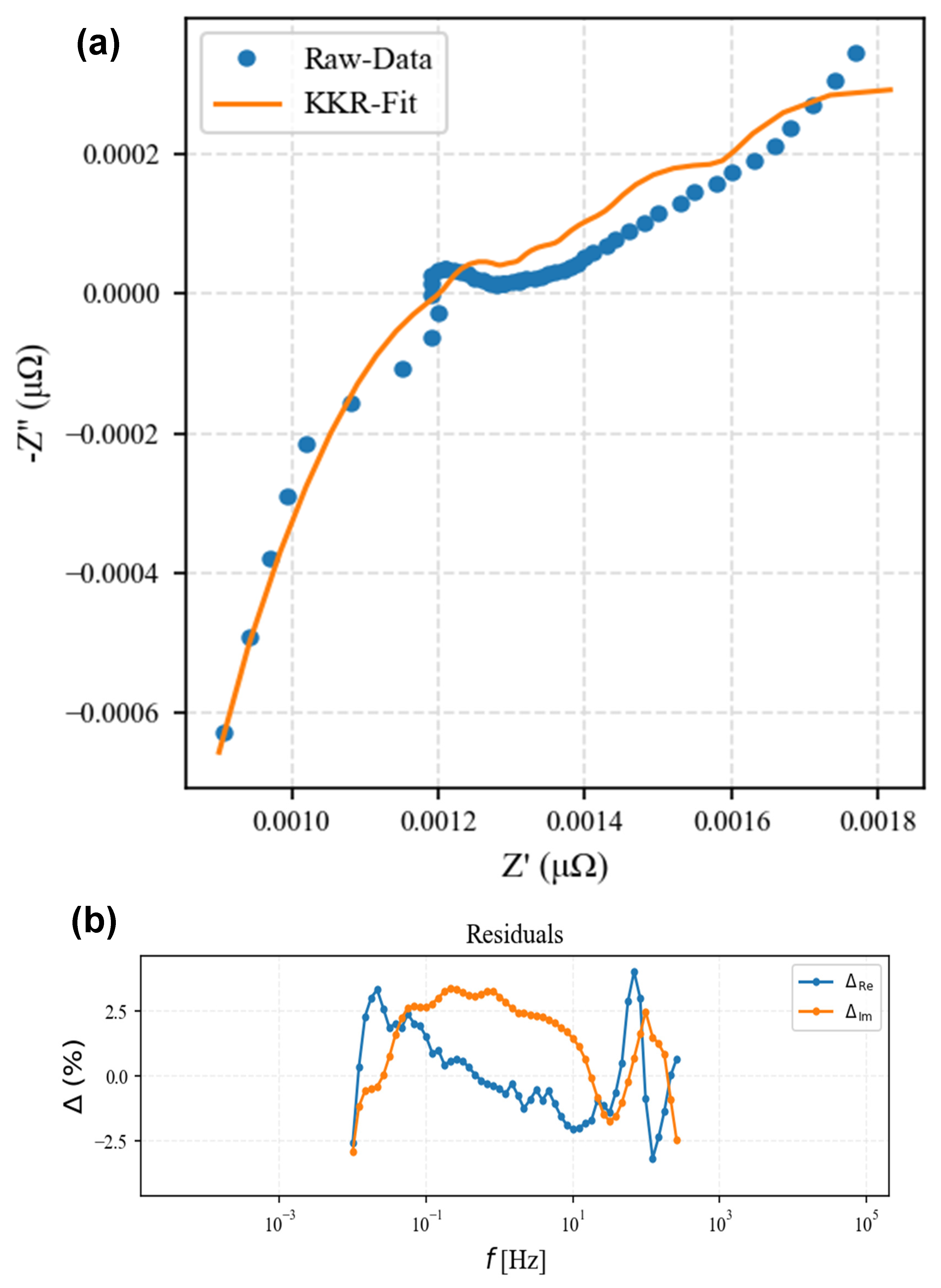
Kramers–Kronig (KK) validation was performed on data acquired using a conventional alligator-clip connection (without the custom fixture). As shown in Appendix B Figure A7, these measurements exhibit larger KK residuals, reaching approximately ±2%–3% across a broad frequency range, with significant frequency-dependent structure. The corresponding Nyquist plot shows noticeable distortion and increased noise in the imaginary component, indicating that contact effects significantly impact the measured impedance. Moreover, the test results could not be reliably reproduced due to variations in contact impedance associated with the alligator clip. In contrast, measurements obtained using the custom fixture exhibit consistently lower KK residuals (as seen in Figure A12) and excellent repeatability (as seen in Figure A6, Figure A7, Figure A8, Figure A9, Figure A10 and Figure A11). These results underscore the critical importance of employing a custom low-impedance fixture to ensure reliable measurements of low-impedance battery cells.
Figure A13. (a) Impedance spectrum (b) KK validation for battery EIS without fixture.
Coatings 16 00930 g0a13

Appendix E. ECM Parameter Sensitivity

Figure A14. ECM model sensitivity analysis for (a) real part (b) imaginary part at 50% SOC, 25 °C.
Coatings 16 00930 g0a14
Figure A15. ECM model sensitivity analysis for (a) real part (b) imaginary part at 100% SOC, 25 °C.
Coatings 16 00930 g0a15
Figure A16. ECM model sensitivity analysis for (a) real part (b) imaginary part at 12% SOC, 40 °C.
Coatings 16 00930 g0a16
Figure A17. ECM model sensitivity analysis for (a) real part (b) imaginary part at 50% SOC, 40 °C.
Coatings 16 00930 g0a17
Figure A18. ECM model sensitivity analysis for (a) real part (b) imaginary part at 100% SOC, 40 °C.
Coatings 16 00930 g0a18

References

  1. Liu, K.; Liu, Y.; Lin, D.; Pei, A.; Cui, Y. Materials for Lithium-Ion Battery Safety. Sci. Adv. 2018, 4, eaas9820. [Google Scholar] [PubMed]
  2. Goodenough, J.B.; Kim, Y. Challenges for Rechargeable Li Batteries. Chem. Mater. 2010, 22, 587–603. [Google Scholar] [CrossRef]
  3. Rezvanizaniani, S.M.; Liu, Z.; Chen, Y.; Lee, J. Review and Recent Advances in Battery Health Monitoring and Prognostics Technologies for Electric Vehicle (EV) Safety and Mobility. J. Power Sources 2014, 256, 110–124. [Google Scholar] [CrossRef]
  4. Gaberšček, M. Understanding Li-Based Battery Materials via Electrochemical Impedance Spectroscopy. Nat. Commun. 2021, 12, 6513. [Google Scholar] [CrossRef] [PubMed]
  5. Farmann, A.; Waag, W.; Sauer, D.U. Adaptive Approach for On-Board Impedance Parameters and Voltage Estimation of Lithium-Ion Batteries in Electric Vehicles. J. Power Sources 2015, 299, 176–188. [Google Scholar] [CrossRef]
  6. Christensen, A.; Adebusuyi, A. Using On-Board Electrochemical Impedance Spectroscopy in Battery Management Systems. In Proceedings of the 2013 World Electric Vehicle Symposium and Exhibition (EVS27); IEEE: New York, NY, USA, 2013; pp. 1–7. [Google Scholar]
  7. Olarte, J.; Martínez de Ilarduya, J.; Zulueta, E.; Ferret, R.; Fernández-Gámiz, U.; Lopez-Guede, J.M. A Battery Management System with EIS Monitoring of Life Expectancy for Lead–Acid Batteries. Electronics 2021, 10, 1228. [Google Scholar] [CrossRef]
  8. Zhang, M.; Liu, Y.; Li, D.; Cui, X.; Wang, L.; Li, L.; Wang, K. Electrochemical Impedance Spectroscopy: A New Chapter in the Fast and Accurate Estimation of the State of Health for Lithium-Ion Batteries. Energies 2023, 16, 1599. [Google Scholar] [CrossRef]
  9. Liu, Y.; Wang, L.; Li, D.; Wang, K. State-of-Health Estimation of Lithium-Ion Batteries Based on Electrochemical Impedance Spectroscopy: A Review. Prot. Control Mod. Power Syst. 2023, 8, 41. [Google Scholar] [CrossRef]
  10. Tatara, R.; Karayaylali, P.; Yu, Y.; Zhang, Y.; Giordano, L.; Maglia, F.; Jung, R.; Schmidt, J.P.; Lund, I.; Shao-Horn, Y. The Effect of Electrode-Electrolyte Interface on the Electrochemical Impedance Spectra for Positive Electrode in Li-Ion Battery. J. Electrochem. Soc. 2018, 166, A5090. [Google Scholar] [CrossRef]
  11. Hu, W.; Peng, Y.; Wei, Y.; Yang, Y. Application of Electrochemical Impedance Spectroscopy to Degradation and Aging Research of Lithium-Ion Batteries. J. Phys. Chem. C 2023, 127, 4465–4495. [Google Scholar] [CrossRef]
  12. Li, S.E.; Wang, B.; Peng, H.; Hu, X. An Electrochemistry-Based Impedance Model for Lithium-Ion Batteries. J. Power Sources 2014, 258, 9–18. [Google Scholar] [CrossRef]
  13. Shao, B.; Zhong, J.; Tian, J.; Li, Y.; Chen, X.; Dou, W.; Liao, Q.; Lai, C.; Lu, T.; Xie, J. State-of-Health Estimation of Lithium-Ion Batteries Based on Electrochemical Impedance Spectroscopy Features and Fusion Interpretable Deep Learning Framework. Energies 2025, 18, 1385. [Google Scholar] [CrossRef]
  14. Zhang, S.; Hosen, M.S.; Kalogiannis, T.; Mierlo, J.V.; Berecibar, M. State of Health Estimation of Lithium-Ion Batteries Based on Electrochemical Impedance Spectroscopy and Backpropagation Neural Network. World Electr. Veh. J. 2021, 12, 156. [Google Scholar] [CrossRef]
  15. Magar, H.S.; Hassan, R.Y.A.; Mulchandani, A. Electrochemical Impedance Spectroscopy (EIS): Principles, Construction, and Biosensing Applications. Sensors 2021, 21, 6578. [Google Scholar] [CrossRef] [PubMed]
  16. Wang, S.; Zhang, J.; Gharbi, O.; Vivier, V.; Gao, M.; Orazem, M.E. Electrochemical Impedance Spectroscopy. Nat. Rev. Methods Primers 2021, 1, 301–350. [Google Scholar] [CrossRef]
  17. Howey, D.A.; Yufit, V.; Mitcheson, P.D.; Offer, G.J.; Brandon, N.P. Impedance Measurement for Advanced Battery Management Systems. In Proceedings of the 2013 World Electric Vehicle Symposium and Exhibition (EVS27); IEEE: Barcelona, Spain, 2013; pp. 1–7. [Google Scholar]
  18. Levi, M.D.; Dargel, V.; Shilina, Y.; Aurbach, D.; Halalay, I.C. Impedance Spectra of Energy-Storage Electrodes Obtained with Commercial Three-Electrode Cells: Some Sources of Measurement Artefacts. Electrochim. Acta 2014, 149, 126–135. [Google Scholar] [CrossRef]
  19. Juarez-Robles, D.; Chen, C.-F.; Barsukov, Y.; Mukherjee, P.P. Impedance Evolution Characteristics in Lithium-Ion Batteries. J. Electrochem. Soc. 2017, 164, A837. [Google Scholar] [CrossRef]
  20. Illig, J.; Schmidt, J.P.; Weiss, M.; Weber, A.; Ivers-Tiffée, E. Understanding the Impedance Spectrum of 18650 LiFePO4-Cells. J. Power Sources 2013, 239, 670–679. [Google Scholar] [CrossRef]
  21. Guo, J.; Li, Y.; Meng, J.; Pedersen, K.; Gurevich, L.; Stroe, D.-I. Understanding the Mechanism of Capacity Increase during Early Cycling of Commercial NMC/Graphite Lithium-Ion Batteries. J. Energy Chem. 2022, 74, 34–44. [Google Scholar] [CrossRef]
  22. Andre, D.; Meiler, M.; Steiner, K.; Wimmer, C.; Soczka-Guth, T.; Sauer, D.U. Characterization of High-Power Lithium-Ion Batteries by Electrochemical Impedance Spectroscopy. I. Experimental Investigation. J. Power Sources 2011, 196, 5334–5341. [Google Scholar] [CrossRef]
  23. Teliz, E.; López-Vázquez, C.; Díaz, V. Degradation Study for 18650 NMC Batteries at Low Temperature. Electrochim. Acta 2024, 475, 143540. [Google Scholar] [CrossRef]
  24. Wang, X.; Wei, X.; Dai, H.; Wu, Q. State Estimation of Lithium Ion Battery Based on Electrochemical Impedance Spectroscopy with On-Board Impedance Measurement System. In Proceedings of the 2015 IEEE Vehicle Power and Propulsion Conference (VPPC); IEEE: New York, NY, USA, 2015; pp. 1–5. [Google Scholar]
  25. Stanciu, T.; Stroe, D.-I.; Teodorescu, R.; Swierczynski, M. Extensive EIS Characterization of Commercially Available Lithium Polymer Battery Cell for Performance Modelling. In Proceedings of the 2015 17th European Conference on Power Electronics and Applications (EPE’15 ECCE-Europe); IEEE: New York, NY, USA, 2015; pp. 1–10. [Google Scholar]
  26. Barai, A.; Chouchelamane, G.H.; Guo, Y.; McGordon, A.; Jennings, P. A Study on the Impact of Lithium-Ion Cell Relaxation on Electrochemical Impedance Spectroscopy. J. Power Sources 2015, 280, 74–80. [Google Scholar] [CrossRef]
  27. Fang, J.; Shen, W.; Cheng, S.H.S.; Ghashghaie, S.; Shahzad, H.K.; Chung, C.Y. Four-Electrode Symmetric Setup for Electrochemical Impedance Spectroscopy Study of Lithium–Sulfur Batteries. J. Power Sources 2019, 441, 227202. [Google Scholar] [CrossRef]
  28. Anderson, E.L.; Bühlmann, P. Electrochemical Impedance Spectroscopy of Ion-Selective Membranes: Artifacts in Two-, Three-, and Four-Electrode Measurements. Anal. Chem. 2016, 88, 9738–9745. [Google Scholar] [CrossRef] [PubMed]
  29. Warburg, E. Ueber Das Verhalten Sogenannter Unpolarisirbarer Elektroden Gegen Wechselstrom. Ann. Der Phys. 1899, 303, 493–499. [Google Scholar] [CrossRef]
  30. Macdonald, D.D. Reflections on the History of Electrochemical Impedance Spectroscopy. Electrochim. Acta 2006, 51, 1376–1388. [Google Scholar] [CrossRef]
  31. Randles, J.E.B. Kinetics of Rapid Electrode Reactions—Discussions of the Faraday Society; RSC Publishing: Cambridge, UK, 1947; Available online: https://pubs.rsc.org/en/content/articlelanding/1947/df/df9470100011 (accessed on 2 May 2025).
  32. Córdoba-Torres, P.; Mesquita, T.J.; Nogueira, R.P. Relationship between the Origin of Constant-Phase Element Behavior in Electrochemical Impedance Spectroscopy and Electrode Surface Structure. J. Phys. Chem. C 2015, 119, 4136–4147. [Google Scholar] [CrossRef]
  33. Lasia, A. The Origin of the Constant Phase Element. J. Phys. Chem. Lett. 2022, 13, 580–589. [Google Scholar] [CrossRef] [PubMed]
  34. Balaguera, E.H.; Allagui, A. Limit Capacitance of the Constant Phase Element. J. Energy Storage 2024, 90, 111801. [Google Scholar] [CrossRef]
  35. Huang, J. Diffusion Impedance of Electroactive Materials, Electrolytic Solutions and Porous Electrodes: Warburg Impedance and Beyond. Electrochim. Acta 2018, 281, 170–188. [Google Scholar] [CrossRef]
  36. Kant, R.; Kumar, R.; Yadav, V.K. Theory of Anomalous Diffusion Impedance of Realistic Fractal Electrode. J. Phys. Chem. C 2008, 112, 4019–4023. [Google Scholar] [CrossRef]
  37. Brett, C.M.A. Electrochemical Impedance Spectroscopy in the Characterisation and Application of Modified Electrodes for Electrochemical Sensors and Biosensors. Molecules 2022, 27, 1497. [Google Scholar] [CrossRef] [PubMed]
  38. Wang, F.; Tang, M. Thermodynamic Origin of Reaction Non-Uniformity in Battery Porous Electrodes and Its Mitigation. J. Electrochem. Soc. 2020, 167, 120543. [Google Scholar] [CrossRef]
  39. Guo, Z.; Ren, X.; Li, L.; He, R.; Gao, Y. Hierarchical Porous Electrode Impedance Model Based on Diffusion Dynamics and the Electrode Morphology and Prediction of Electric Double-Layer Structures. ACS Appl. Energy Mater. 2023, 6, 508–518. [Google Scholar] [CrossRef]
  40. Bisquert, J.; Compte, A. Theory of the Electrochemical Impedance of Anomalous Diffusion. J. Electroanal. Chem. 2001, 499, 112–120. [Google Scholar] [CrossRef]
  41. Brug, G.J. The Analysis of Electrode Impedances Complicated by the Presence of a Constant Phase Element. J. Electroanal. Chem. Interfacial Electrochem. 1984, 176, 275–295. [Google Scholar] [CrossRef]
  42. Franceschetti, D.R.; Macdonald, J.R.; Buck, R.P. Interpretation of Finite-Length-Warburg-Type Impedances in Supported and Unsupported Electrochemical Cells with Kinetically Reversible Electrodes. J. Electrochem. Soc. 1991, 138, 1368–1371. [Google Scholar] [CrossRef]
  43. Diard, J.-P.; Le Gorrec, B.; Montella, C. Linear Diffusion Impedance. General Expression and Applications. J. Electroanal. Chem. 1999, 471, 126–131. [Google Scholar] [CrossRef]
  44. Jorcin, J.-B.; Orazem, M.E.; Pébère, N.; Tribollet, B. CPE Analysis by Local Electrochemical Impedance Spectroscopy. Electrochim. Acta 2006, 51, 1473–1479. [Google Scholar] [CrossRef]
  45. Montero-Rodríguez, J.; Schroeder, D.; Krautschneider, W.; Starbird, R. Equivalent Circuit Models for Electrochemical Impedance Spectroscopy of PEDOT-Coated Electrodes. In Proceedings of the 6th IEEE Germany Student Conference; IEEE: New York, NY, USA, 2015. [Google Scholar]
  46. González, F.; Greiner, D.; Mena, V.; Souto, R.M.; Santana, J.J.; Aznárez, J.J. Fitting Procedure Based on Differential Evolution to Evaluate Impedance Parameters of Metal–Coating Systems. Eng. Comput. 2019, 36, 2960–2982. [Google Scholar] [CrossRef]
  47. Zhang, L.; Wang, X.; Dai, H.; Wei, X. A Novel Fitting Method of Electrochemical Impedance Spectroscopy for Lithium-Ion Batteries Based on Random Mutation Differential Evolution Algorithm. SAE Int. J. Electrified Veh. 2022, 11, 231–246. [Google Scholar] [CrossRef]
  48. Sardar, S.A.; Iqbal, S.; Park, J.; Han, S.; Kim, W.Y. Field Data Retrieval for Electric Vehicles and Estimating Equivalent Circuit Model Parameters via Particle Swarm Optimization. Technologies 2025, 13, 91. [Google Scholar] [CrossRef]
  49. Habte, B.T.; Jiang, F. Effect of microstructure morphology on Li-ion battery graphite anode performance: Electrochemical impedance spectroscopy modeling and analysis. Solid State Ion. 2018, 314, 81–91. [Google Scholar] [CrossRef]
  50. Kazilas, M.C.; Skordos, A.A.; Partridge, I.K. Parameter Estimation in Equivalent Circuit Analysis of Dielectric Cure Monitoring Signals Using Genetic Algorithms. Inverse Probl. Sci. Eng. 2005, 13, 157–176. [Google Scholar] [CrossRef]
  51. Kubisa, S.; Warsza, Z.L. Identification of Parameters of the Capacitor Equivalent Scheme Using Monte Carlo Methods. In Proceedings of the Automation 2017; Szewczyk, R., Zieliński, C., Kaliczyńska, M., Eds.; Springer International Publishing: Cham, Switzerland, 2017; pp. 165–177. [Google Scholar]
  52. Frazier, P.I. A Tutorial on Bayesian Optimization. arXiv 2018, arXiv:1807.02811. [Google Scholar]
  53. EVSpecification. 2023 Volkswagen ID.4 Pro S—Specification and Price. 2025. Available online: https://www.vw.com/en/models/id-4.html (accessed on 19 June 2026).
  54. Gamry Instrument. Interface 5000P Potentiostat/Galvanostat/ZRA Operator’s Manual; Gamry Instrument: Warminster, PA, USA, 2021. [Google Scholar]
  55. Schönleber, M.; Klotz, D.; Ivers-Tiffée, E. A Method for Improving the Robustness of Linear Kramers-Kronig Validity Tests. Electrochim. Acta 2014, 131, 20–27. [Google Scholar] [CrossRef]
  56. Long, T.; Wang, L.; Kan, C.-D.; Lee, J.D.; Long, T.; Wang, L.; Kan, C.-D.; Lee, J.D. Online Hyperparameter Tuning in Bayesian Optimization for Material Parameter Identification: An Application in Strain-Hardening Plasticity for Automotive Structural Steel. AppliedMath 2026, 6, 6. [Google Scholar] [CrossRef]
  57. Gao, F.; Han, L. Implementing the Nelder-Mead Simplex Algorithm with Adaptive Parameters. Comput. Optim. Appl. 2012, 51, 259–277. [Google Scholar] [CrossRef]
  58. Nogueira, F. Bayesian Optimization: Open Source Constrained Global Optimization Tool for Python. 2014. Available online: https://github.com/bayesian-optimization/bayesianoptimization (accessed on 19 June 2026).
  59. Virtanen, P.; Gommers, R.; Oliphant, T.E.; Haberland, M.; Reddy, T.; Cournapeau, D.; Burovski, E.; Peterson, P.; Weckesser, W.; Bright, J.; et al. SciPy 1.0: Fundamental Algorithms for Scientific Computing in Python. Nat. Methods 2020, 17, 261–272. [Google Scholar] [CrossRef] [PubMed]
  60. De Ath, G.; Fieldsend, J.E.; Everson, R.M. What Do You Mean? The Role of the Mean Function in Bayesian Optimisation. arXiv 2020, arXiv:2004.08349. [Google Scholar]
  61. Rasmussen, C.E.; Williams, C.K.I. Gaussian Processes for Machine Learning; The MIT Press: Cambridge, MA, USA, 2005; ISBN 978-0-262-18253-9. [Google Scholar]
  62. Long, T.; Wang, L.; Kan, C.-D.; Lee, J.D.; Long, T.; Wang, L.; Kan, C.-D.; Lee, J.D. A Novel Approach for Modeling Strain Hardening in Plasticity and Its Material Parameter Identification by Bayesian Optimization for Automotive Structural Steels Application. AppliedMath 2025, 5, 104. [Google Scholar] [CrossRef]
  63. Wu, L.; Gong, Y.; Song, S.; Zhao, Y.; Wang, X.; Li, F.; Tang, X.; Sun, Y.; Zhang, X.; Sun, X.; et al. Low-Frequency Characteristics and Fractional-Order Impedance Model for Electrochemical Impedance Spectroscopy in Large-Capacity Lithium-Ion Batteries. J. Energy Storage 2025, 134, 118222. [Google Scholar] [CrossRef]
  64. Huber, P.J. Robust Estimation of a Location Parameter. In Breakthroughs in Statistics: Methodology and Distribution; Kotz, S., Johnson, N.L., Eds.; Springer: New York, NY, USA, 1992; pp. 492–518. ISBN 978-1-4612-4380-9. [Google Scholar]
  65. Ma, J.; Wang, H.; Zheng, C.; Tao, Z.; Fu, Y.; Bai, H.; Xiao, H. Effects of Temperature on the Parameters of the Electrochemical Impedance Spectroscopy for Lithium-Ion Batteries. J. Phys. Conf. Ser. 2023, 2557, 012028. [Google Scholar] [CrossRef]
  66. Santoni, F.; De Angelis, A.; Moschitta, A.; Carbone, P.; Galeotti, M.; Cinà, L.; Giammanco, C.; Di Carlo, A. A Guide to Equivalent Circuit Fitting for Impedance Analysis and Battery State Estimation. J. Energy Storage 2024, 82, 110389. [Google Scholar] [CrossRef]
  67. Barai, A.; Uddin, K.; Widanage, W.D.; McGordon, A.; Jennings, P. A Study of the Influence of Measurement Timescale on Internal Resistance Characterisation Methodologies for Lithium-Ion Cells. Sci. Rep. 2018, 8, 21. [Google Scholar] [CrossRef] [PubMed]
  68. He, R.; He, Y.; Xie, W.; Guo, B.; Yang, S. Comparative Analysis for Commercial Li-Ion Batteries Degradation Using the Distribution of Relaxation Time Method Based on Electrochemical Impedance Spectroscopy. Energy 2023, 263, 125972. [Google Scholar] [CrossRef]
  69. Ezpeleta, I.; Freire, L.; Mateo-Mateo, C.; Nóvoa, X.R.; Pintos, A.; Valverde-Pérez, S. Characterisation of Commercial Li-Ion Batteries Using Electrochemical Impedance Spectroscopy. ChemistrySelect 2022, 7, e202104464. [Google Scholar] [CrossRef]
  70. Meddings, N.; Heinrich, M.; Overney, F.; Lee, J.-S.; Ruiz, V.; Napolitano, E.; Seitz, S.; Hinds, G.; Raccichini, R.; Gaberšček, M.; et al. Application of Electrochemical Impedance Spectroscopy to Commercial Li-Ion Cells: A Review. J. Power Sources 2020, 480, 228742. [Google Scholar] [CrossRef]
  71. Morali, U.; Erol, S. Analysis of Electrochemical Impedance Spectroscopy Response for Commercial Lithium-Ion Batteries: Modeling of Equivalent Circuit Elements. Turk. J. Chem. 2020, 44, 602–613. [Google Scholar] [CrossRef] [PubMed]
  72. Deleebeeck, L.; Veltzé, S. Electrochemical Impedance Spectroscopy Study of Commercial Li-Ion Phosphate Batteries: A Metrology Perspective. Int. J. Energy Res. 2020, 44, 7158–7182. [Google Scholar] [CrossRef]
  73. Erol, S. Equivalent Circuit Model for Electrochemical Impedance Spectroscopy of Commercial 18650 Lithium-Ion Cell Under Over-Discharge and Overcharge Conditions. Electroanalysis 2024, 36, e202300232. [Google Scholar] [CrossRef]
  74. Gamry Instrument. EIS: Potentiostatic or Galvanostatic Mode? Gamry Instrument: Warminster, PA, USA, 2025. [Google Scholar]
Figure 1. Schematic workflow of fixture-assisted four-terminal EIS characterization and ECM analysis for a low-impedance EV pouch cell, including controlled EIS measurement, KK−based data−quality validation, and BO−NM parameter identification with an LM benchmark.
Coatings 16 00930 g001
Figure 2. NCM712 cell is connected to EIS analyzer with 4-terminal sensing method.
Coatings 16 00930 g002
Figure 3. Gamry 5000P potentiostat/galvanostat interface with Arbin battery cycle (left).
Coatings 16 00930 g003
Figure 4. Cell terminal connection fixture.
Coatings 16 00930 g004
Figure 5. Equivalent circuit model for EV cells in study.
Coatings 16 00930 g005
Figure 6. Typical linear Kramers–Kronig validation of experimental EIS at 12% SOC and 25 °C: (a) Nyquist plot with an enlarged view; (b) frequency-dependent relative residuals of the real and imaginary impedance components; and (c) overall relative error as a function of the number of parallel RC elements.
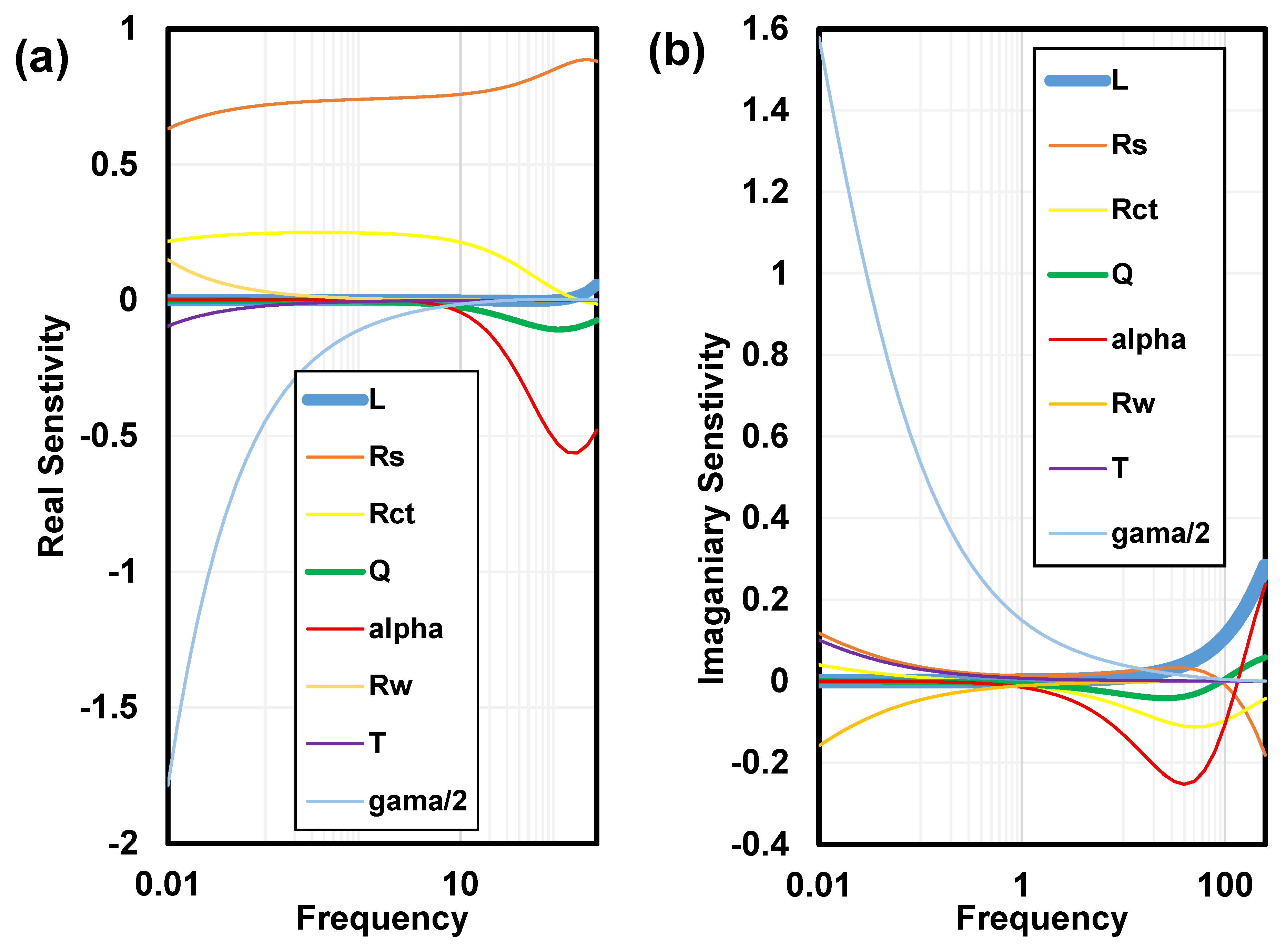
Coatings 16 00930 g006
Figure 7. Nyquist plot and ECM fitting results (a) and Bode plots (b,c) for three repeated EIS tests of an EV cell at 12% SOC and 25 °C. Standard deviation (SD) is calculated from 3 repeated tests at each frequency point.
Coatings 16 00930 g007
Figure 8. Nyquist plot and ECM fitting results (a) and Bode plots (b,c) for 4 repeated EIS tests of an EV cell at 50% SOC and 25 °C. Standard deviation (SD) is calculated from 4 repeated tests at each frequency point.
Coatings 16 00930 g008
Figure 9. Nyquist plot and ECM fitting results (a) and Bode plots (b,c) for 4 repeated EIS tests of an EV cell at 100% SOC and 25 °C. Standard deviation (SD) is calculated from 4 repeated tests at each frequency point.
Coatings 16 00930 g009
Figure 10. Nyquist plot and ECM fitting results (a) and Bode plots (b,c) for 4 repeated EIS tests of an EV cell at 12% SOC and 40 °C. Standard deviation (SD) is calculated from 4 repeated tests at each frequency point.
Coatings 16 00930 g010
Figure 11. Nyquist plot and ECM fitting results (a) and Bode plots (b,c) for 4 repeated EIS tests of an EV cell at 50% SOC and 40 °C. Standard deviation (SD) is calculated from 4 repeated tests at each frequency point.
Coatings 16 00930 g011
Figure 12. Nyquist plot and ECM fitting results (a) and Bode plots (b,c) for 4 repeated EIS tests of an EV cell at 100% SOC and 40 °C. Standard deviation (SD) is calculated from 4 repeated tests at each frequency point.
Coatings 16 00930 g012
Figure 13. Bayesian optimization (BO) and Nelder–Mead (NM) simplex optimization convergence history.
Coatings 16 00930 g013
Figure 14. ECM parameter sensitivity study based on 1% perturbation on 12% SOC at 25 °C. (a) The real part sensitivity, (b) The imaginary part sensitivity.
Coatings 16 00930 g014
Figure 15. Nyquist plots of EIS test data and ECM fitting results for “Cell 7” at 25 °C (a) and 40 °C (b). The percentage in each label denotes the state of charge, and the number at the end denotes the repeated test number of the same testing condition.
Coatings 16 00930 g015
Table 2. SOC, Temperature, number of repeats, and OCV for each experiment. Unit: volt.
TemperatureSOC1234ΔOCV
25 °C12%3.5927143.5941893.590987 0.003202
50%3.6548013.6527623.6510863.6493750.005426
100%4.0646474.0621874.0597184.0547210.009926
40 °C12%3.5917653.589893.5883173.5863460.005419
50%3.6512473.6496443.6459763.6444130.006834
100%4.0763174.0736894.0707374.0682830.008034
Table 3. Electric components in equivalent circuit model.
NameSymbolImpedance
Inductance L Z L = j ω L
Solution resistance R s Z R s = R s
Charge-transfer resistance R c t Z R c t = R c t
Constant phase element C P E Z C P E = 1 / Q j ω α
Generalized Warburg W 1 Z W G = R w ( j T ω ) γ / 2 coth [ ( j T ω ) γ / 2 ]
Battery ECM Z E C M Z E C M = Z L + Z R s + 1 1 Z C P E + 1 Z R c t   +   Z W G
Table 4. Average standard deviation for repeated tests on the same condition for “Cell 7”.
12% SOC 25 °C50% SOC 25 °C100% SOC 25 °C12% SOC 40 °C50% SOC 40 °C100% SOC 40 °C
Repeated tests344444
S D ¯ Z (mΩ)3.1130 × 10−33.7829 × 10−36.1336 × 10−35.5275 × 10−32.9744 × 10−32.8596 × 10−3
S D ¯ θ (Degree)8.9629 × 10−28.8745 × 10−21.0895 × 10−11.1894 × 10−19.5011 × 10−21.0643 × 10−1
Table 5. ECM parameters fit by BO + Nelder–Mead.
ECM Parameter Fit by BO (Unit)12% SOC 25 °C50% SOC 25 °C100% SOC 25 °C12% SOC 40 °C50% SOC 40 °C100% SOC 40 °C
L ( H ) 2.0454 × 10⁻⁷
R s (Ω)1.0186 × 10−39.9411 × 10−49.9609 × 10−49.4680 × 10−49.8900 × 10−49.6912 × 10−4
R c t (Ω)3.3843 × 10−42.1081 × 10−42.1467 × 10−41.2492 × 10−45.3384 × 10−53.2149 × 10−5
Q ( Ω 1 s α ) 22.506
α 0.76824
R w (Ω)25.30734.77321.54520.51834.97321.767
T ( s ) 7.9847 × 1082.1592 × 1093.7968 × 1093.5104 × 1091.9761 × 10103.3041 × 1010
γ / 2 0.632460.613130.564780.577070.553690.51469
Residual2.14 × 10−32.73 × 10−32.89 × 10−32.77 × 10−32.43 × 10−32.54 × 10⁻³
Disclaimer/Publisher’s Note: The statements, opinions and data contained in all publications are solely those of the individual author(s) and contributor(s) and not of MDPI and/or the editor(s). MDPI and/or the editor(s) disclaim responsibility for any injury to people or property resulting from any ideas, methods, instructions or products referred to in the content.