Abstract
We implemented deep learning models to examine the accuracy of predicting a single feature (sheet resistance) of thin films of indium-doped zinc oxide deposited via plasma sputter deposition by feeding the spectral data of the plasma to the deep learning models. We carried out 114 depositions to create a large enough dataset for use in training various artificial neural network models. We demonstrated that artificial neural networks could be implemented as a model that could predict the sheet resistance of the thin films as they were deposited, taking in only the spectral emission of the plasma as an input with the objective of taking a step toward digital manufacturing in this area of material engineering.
1. Introduction
Transparent conductive oxides (TCO) are materials which have attracted a significant amount of attention due to their vast application areas. They are an essential part of various optoelectronic devices, such as light emitting diodes (LEDs), thin-film solar cell modules, flat panel displays and flexible electronics. Physical vapor deposition (sputtering) under vacuum is one of the proven industrial methods of depositing thin films of these materials [1]. During the sputter deposition of materials, the sputtering conditions govern the way that the atoms are deposited and laid on the substrate surface as a thin film coating. The arrangement of the atoms in materials such as TCOs will ultimately define the work function, electron affinity, band-gap and all relevant functional parameters of the as-deposited material. Unlike standard laboratory chemical reactions, which give significant parameters of choice to alter during the reaction, the plasma sputter deposition technique can only be altered in terms of the operating chamber pressure, plasma power, the trajectory angle of sputtered atoms and distance between the magnetron and the substrate surface, etc. For example, researchers who apply this technique for TCO preparation usually report their findings by stating the condition of the sputtering process, such as chamber pressure, plasma power and the gas composition of the chamber during deposition. Furthermore, when moving from one sputter machine to another, depending on the dimensions of the chamber, size of the targets and a few other design related issues, TCO coatings with different properties can be obtained, even if the sputtering conditions are maintained, according to an earlier report. As such, to achieve a particular thin film with certain features and functionality, multiple trial and error experimental runs are required to fine tune a machine to produce a specific desired coating. This means that, to fully digitize the sputter deposition process, significant constrains will arise. This study focused on the spectral emissions of the plasma, using them to predict the properties of the thin films deposited via the process. Certainly, the plasma in the sputtering procedure is the core of the reaction and fundamental to the deposition of the thin film. However, characterizing a plasma through optical spectroscopy is nothing new [2,3,4,5,6,7,8]. The diagnosis of laboratory plasma is usually carried out by optical emission spectroscopy (OES), through which numerous analytical techniques are established to determine certain plasma properties, such as electron density, plasma temperature, element recognition and qualification of elements present in the plasma.
Such fundamental plasma physics-related investigations are complex; extensive expertise, as well as time and effort, are required to assess them. We briefly looked into the concept of the plasma temperature calculation to appreciate these complexities.
The radiative behaviour of the atomic constituents of any plasma can only be predicted if the expected population of its possible states are known and the atoms obey the Boltzmann distribution for every possible state and radiation energy density to assume a thermal equilibrium condition is present [4,5,6,7,8,9]. However, creating such a condition in the laboratory would be almost impossible. As such, the concept of local thermal equilibrium (LTE) condition was considered. LTE can be described as a state where Boltzmann and Saha equations, which govern the distribution of energy level excitation and ionization temperature, are equal to the Maxwell–Boltzmann distribution of free electron velocities [8,9,10]. Achieving the LTE condition depends on defining the plasma by a common temperature T and the existence of sufficient large electron density. McWhirter proposed a criterion where there is a need for a critical amount of electron density for LTE conditions to exist [11,12,13,14].
The temperature of ions and electrons in the plasma are directly proportional to their random average kinetic energy, while Maxwell distribution governs the distribution of velocities for each particle when thermal equilibrium conditions apply. Under the LTE conditions, the same temperature is assumed for electrons, ions and atoms in the plasma and the plasma temperature is (considered) the temperature of the electrons [4].
From the plasma spectral emissions, two spectral lines can be chosen from the same species (for example argon) and ionization stage, where there is a large difference in the upper energy level. Ultimately, by taking a ratio (I1)/(I2) of the intensities of the selected lines, the temperature of the electron can be calculated in electron volts [15].
This method is the simplest method of calculating the temperature of the plasma and its accuracy is conditional on using two lines with a maximum difference in their upper energy states.
Another feature of the plasma: the electron density can be calculated using various methods, two of which are (1) applying the Stark broadening relationships or (2) applying the Saha-Boltzmann equation. The Stark broadening is caused by the electric field of electrons and ions interfering, which results in the broadening of the spectral line. The interference of the mentioned electric fields causes fluctuations in the field of plasma as the radiating atoms are surrounded by the interfering electrons and ions. The electric field of the electrons or ions causes a perturbation of energy levels close to the continuum while simultaneously affecting the external applied electric field—which ultimately causes the observed spectral broadening [15,16,17].
2. Modelling Background
Since the 1980s, there have been many attempts to model the magnetron sputtering discharge. These models can be classified into purely mathematical models or analytical models. Theoretical models can be subclassified into kinetic models, fluid models or plasma physics-based models. These models need to include the calculations of the electric field based on the applied external voltage and distribution of the charged plasma species. The sputtering process can be classified into three stages: ejection of the particles from the target, particle transport and, finally, condensation on the substrate surface. This means the complete model of this process needs to describe discharge physics, plasma physics and material surface interactions. Some of the models that have been implemented to date are summarized as follows:
- 1.
- Analytical models rely on simple analytical formulae to describe the behaviour of the glow discharge parameters, such as the current and voltage. They are simple and easy to calculate; however, they suffer from accuracy and are only applicable for limited ranges of deposition conditions [16].
- 2.
- Pathway models are based on a simple approach of following the sputtered and working gas species within the discharge to gain understanding of the discharge processes in pulsed magnetron sputtering discharges. It was originally developed to determine the ionized fraction of the film-forming material arriving at the substrate and to explain the low deposition rate observed in some discharges [17].
- 3.
- Fluid models define the plasma as a continuum and are based on continuity and transport equations for the various discharge species, along with the Poisson equation, in order to obtain a self-consistent electric field distribution. The fluid model has an advantage in terms of easy computing. However, the validity of using a fluid model to describe a magnetron sputtering discharge has been questioned [18].
- 4.
- Ionization region models are based on defining an ionization region which is volume-averaged and time dependent. The region is the visually observed bright glowing plasma near the surface of the target. Via this model, the time evolution of neutral and charged species and the electron temperature in pulsed magnetron sputtering discharges can be calculated. The model is constrained by experimental parameter inputs—such as the geometry and the working gas pressure, the working gas, sputter yields and target species—and a reaction system setup for these species, in the sense that it first needs to be adapted to an existing discharge and then fitted using two or three parameters to reproduce the measured discharge current and voltage waveforms [19,20].
- 5.
- Hybrid models, as the name suggests, intend to combine the precision of kinetic models with the computational simplicity of the fluid model. In the magnetron sputtering discharge, the secondary electrons are emitted from the cathode target surface and accelerated to high energies within the cathode sheath. Often, the electrons are split up into two groups: the so-called fast electrons, with energy above the threshold for inelastic collisions, which are treated with a kinetic Monte Carlo model, and slower electrons that are described with a fluid model. In the hybrid approach, the ions and bulk electrons are treated by the fluid description and the fast electrons are treated by the particle model [21]. However, this approach has been criticised by Kolev and Bogaerts [22].
- 6.
- In Direct Monte Carlo simulations, several test particles, representing many plasma species, are followed. The movement of the test particles is influenced by applied forces and collisions with other particles. Direct Monte Carlo simulations have been used to predict the spatial distribution of the ionization [23] and ion trajectories [24] in a planar magnetron sputtering discharge.
- 7.
- Boltzmann solver is based on numerically solving the Boltzmann equation to obtain the electron energy distribution within the discharge. This is an accurate and widely implemented model in discharge physics. However, in the magnetron sputtering discharge, the Boltzmann equation includes a Lorentz force term that leads to mathematical complexity. Therefore, this approach has only been applied successfully in the case of a cylindrical magnetron sputtering discharge that consisted of a coaxial inner cathode and an outer anode [25,26,27,28].
- 8.
- Monte Carlo collisional simulations are based on the same principle as the discussed Monte Carlo simulations. The trajectories of many individual species are calculated applying Newton’s laws, and their collisions are treated by assigning random numbers [29]. Furthermore, the electric field distribution is also calculated self-consistently from the positions of the charged species using the Poisson equation. This approach provides spatial distribution of the charged particles projected onto a grid, along with the electric field across the discharge, illustrating charge density distribution, from which the electric field distribution can be calculated. It is the most powerful numerical method to explore the magnetron sputtering discharge. However, it relies on significant computational power as it tries to describe the detailed behaviour of charged species along with solving the Poisson equation [30].
All of these are methods that require precise expertise in the field of plasma physics and statistical mechanics. However, at operational levels and where industrial scale deposition is considered, such an extensive and detailed knowledge of plasma physics and implementation of complex mathematical models will be impossible to implement.
Furthermore, the ionization processes in magnetron sputtering discharges seem not to be uniformly distributed along the racetrack. Magnetron sputtering processes are known to demonstrate inhomogeneous plasma with distinct regions of increased light intensity that seem to float along the racetrack. The appearance of rotating dense plasma, referred to as spokes, have been known for a few decades [31,32,33].
The spokes are independent of the magnetron configuration and have been observed with both circular and rectangular or linear magnetron targets [34,35,36,37]. As such, the plasma may seem inhomogeneous.
These inhomogeneities smooth out at high discharge currents to yield azimuthally homogeneous plasma [38,39], where power densities are above 3 kW·cm2. The reason for this observation can be explained through electron heating, resulting from a combination of acceleration of secondary electrons and pure Ohmic heating [40].
At the same time, the addition of a reactive gas leads to compound formation on the target surface, referred to as surface poisoning, which affects other parameters of the sputtering discharge, such as the secondary electron emission yield, the sputter yield, and the plasma composition near the target. It can even lead to alternation of the spoke shape [41] and decrease of discharge voltage upon addition of reactive gas, which can be correlated with an increase in the secondary electron emission [42,43].
In addition to instabilities propagating along the target surface (i.e., spokes), the plasma may also exhibit other instabilities. In particular, the plasma can oscillate in a direction normal to the target surface, which has been termed breathing instability [44,45]. Spokes and breathing instability usually superimpose [44].
Electrons arriving at a spoke reach a region of higher potential, and are thus energized, enabling them to cause localized excitation and ionization. This suggests that images of spokes can be taken as approximate images of the potential distribution [46]. Recent measurements by Held et al. indicated that the spokes had a higher plasma density, electron temperature and plasma potential than the surrounding plasma [47].
2.1. A New Approach
The objective of this article and our research was to push all the mentioned complexities into the black box of an artificial neural network. With modern computing powers and artificial intelligence (AI)-based data assessment methodologies, we aimed to explore implementing an alternative approach in plasma diagnostics during the sputter deposition process to assess the qualitative parameters of thin films as they were deposited. We believe that artificial intelligence and deep learning can be the answer, if the objective is to fully automate and digitise the industrial-scale sputtering process.
Artificial Neural Networks (ANNs) are the core of deep learning. They are powerful, scalable, versatile and highly complex, yet easy to implement with high level application programming interfaces (APIs) such as KERAS and TENSORFLOW in Python programming language. The origins of ANNs can be dated back to the 1940s; however, their complexity and subsequent need of powerful computing restricted their application. Today, with the emergence of modern powerful and fast computers and commercial entities such as Google and Facebook, along with the availability of large digital databanks, we are observing an explosive emergence of ANNs and they are outperforming all existing machine learning models that were once ahead in terms of popularity and application, such as support vector machines (SVM). Some theoretical limitations associated with ANNs, such as the model getting locked in local minima of a function, seem to be benign in practice. In fact, multidimensional data with their complex function gradients are least affected by the local minima restriction.
The unit constructs of ANNs are supposedly a mimic of biological neurons and their interactive connections. However, the mysterious and extremely complex nature of biological neurons is at another level of excellence yet to be explored by neurologists. As such, the term neuron as used in describing ANNs is only a term used for description purposes. The term perceptron for each unit is a more realistic description of the ANNs constituents. The perceptron was invented in 1957 by Frank Rosenblatt. The perceptron computes a weighted sum of its inputs and applies a function to the weighted sum. Figure 1 illustrates the basic mathematical operation of a single preceptron. For an in depth understanding of artifical neural networks and deep learning, see [48,49].
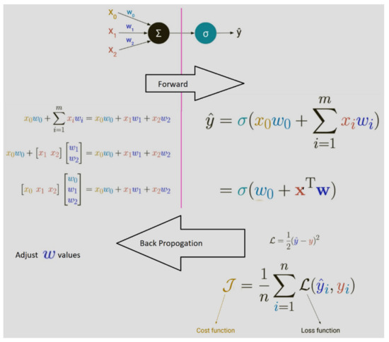
Figure 1.
A simple representation of the operation of single perceptron fed with three data (X0,X1,X2) inputs to give an output (ŷ) which needs to be close to a known (y) value. The perceptron will apply weights to the inputs, sum up and apply a function (σ) on the outcome, and will adjust the weights through a forward and backward loop by implementing a loss function (error factor) until the selected weights result in ŷ being as close as possible to y value.
Ultimately, ANNs are a multilayer of perceptron’s constituting input layers, hidden layers and output layers. When an ANN contains a deep stack of hidden layers, it is referred to as a deep neural network (DNN).
The idea is to feed multi-dimensional data (vector) via the input neurons of a DNN leading to an output value from the output layers. This output will be simultaneously compared with experimental outputs and the model will train itself by adjusting the weights (Figure 2) associated with the perceptron at each layer. The model learns through the process of back propagation, introduced by David Rumelhart [49], which in its core implements Gradient Descent to compute the gradient of the networks error. Detailed discussion of the theory and mechanism of deep learning is beyond the scope of this article, as it is an exponentially growing field in computer science and artificial intelligence. In this article, we explored the feasibility of implementing deep learning models as a step toward digitising the sputtering process.
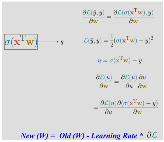
Figure 2.
A simplified illustration of the backpropagation process and adjustment of weights by a perceptron. New weights are calculated by subtracting the old weight from the product of the learning rate and the derivative of the loss function.
The concept of this experimental trial is illustrated in Figure 3, where, during the deposition of the films, the spectral data from the plasma was gathered. Once the deposition was complete, the sheet resistance of the film was calculated via a four-point probe measurement system.
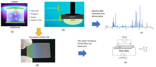
Figure 3.
Illustration of the sputtering process and the experimental concept. Spectral data of the plasma is collected during the deposition process and the sheet resistance of the deposited films are measured. σ is the sheet resistance, V: voltage, I: current, w is the width and L is the length of sample region to be measured. (a) is illustrating plasma deposition; (b) is illustrating the method by which spectral data were collected via a collimator and optical fibre; (c) is the spectral data; (d) is a sample substrate coated with the thin film; (e) represents the method of sheet resistance calculation.
In our experiments, the spectral emissions at each 0.2 nm of the spectral data or area under emission peaks at 100 nm intervals acted as the ‘x’ values described in Figure 1 and the sheet resistance of the film served as the ‘y’ value.
2.2. ANN Modelling
Figure 4 visualises the theoretical concept of our experiments with direct ANN models. The spectral data, in form of the vectors containing the area under the peaks in linearly spaced 100 nm spectral gaps or in the form of vectors composed of emission intensity at each 0.2 nm interval segment of the plasma spectrum, were fed into a deep network of perceptrons (neurons). The actual sheet resistance of the films associated with each spectral data vector was also fed into the neural network to enable the learning process of the model.
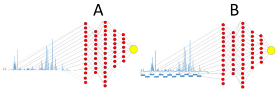
Figure 4.
Illustration of the theoretical concept. (A) In this approach, spectral data of the plasma in form of point-by-point spectral intensity values are fed into a neural network model and (B) in this approach, spectral data of the plasma in the form of area under the peaks at certain intervals (50 nm windows) are fed into a neural network model. The model is also fed with the sheet resistance values, physically measured to enable the model to learn from the spectral data to predict the sheet resistance value. (The shape and size of the neural network does not represent the actual models developed and is only for illustration).
Once the model was trained, it was provided with spectral data without film sheet resistance to predict the conductivity of the film, purely based on the spectral emissions of the plasma as the film was being deposited.
2.3. CNN Modelling
In a separate attempt, we converted the spectral data of the plasma emission into an image by converting the emission intensity vectors into a matrix. This matrix could then be converted into an image where each spectral data point acted as a pixel of the image. We then used these images to train a convolutional neural network model and predicted the sheet resistance of the films associated with each deposition. Convolution is a mathematical operation wherein a signal is convolved with a kernel and, in CNNs, it technically reflects implementing a cross-correlation. The kernels (of filter maps) extracted feature maps from the signal. In our experiments, the spectrum of the plasma was converted into an image and, using various random kernels in a CNN model, features were extracted from the image and ultimately used for regression analysis when they were converted into a flat single vector (see Figure 5). These kernels were initially randomly chosen during the model training and were learned through a gradient descent process. Ultimately, the convolutional approach was intended to reduce the data size and focus on important features from the data. Discussing the mathematics and structure of these models was beyond the scope of this work; however, for further reading refer to [50,51,52,53].

Figure 5.
Illustration of implementation of a convolutional neural network linked to a regression multilayer ANN model for predicting the sheet resistance of the thin films from an image generated from the spectral emission of the plasma.
3. Experimental
Deep learning requires large data banks. Data, in the form of feature columns and expected output columns in large quantities, are required for training these models. As such, the main task of our research was to gather a large enough data bank by continuously operating a sputtering deposition system, obtaining spectral data and measuring an output value associated with the samples prepared during the experiments—in this case, the sheet resistance of the thin films. The data implemented in this article were the result of continuous operation of a machine over a period of one year. Thanks to the ongoing extensive research conducted by data science researchers who have advanced the progress on deep learning models, these models are now powerful and easy to implement. Nonetheless, large datasets are fundamental to their implementation and, as such, data acquisition remained at the core of this research.
3.1. The Instruments
The sputtering instrument used for these experiments was a V6000 unit that was manufactured by Scientific Vacuum Systems limited (SVS Ltd., Wokingham, UK) with a vacuum chamber of ~40 cm × 40 cm × 40 cm dimesnsion with three 6” confocal magnetrons holding targets of the choice materials to be deposited. The distance between the target surface and substrate (centre to centre) was 15 cm at 45° angle. The working gas used in the experiment was a 95% argon −5% hydrogen (Ar + H) single-source mixed-gas cylinder.
During each deposition procedure, spectral data from the plasma was obtained by placing an in-vacuum collimator optic probe (Plasus GmbH, Mering, Germany) at a right angle to the glow of the plasma. The probe was installed on the magnetron so that it horizontally collected light from ~1.5 cm away from the surface of the target and at 4 cm from the edge of the target. The collected light was then guided to a Plasus Emicon Spectrometer (Mering, Germany), which generated a detailed spectral plot of the emission. Emicon software (Plasus GmbH, Mering, Germany) coupled to the spectrometer logged the spectral data of the plasma and was also programmed to calculate the area under the peak of the spectral window segments (see Figure 4). A Jeti Specbos 1201 spectrometer (Jena, Germany) was used as secondary spectral monitoring system.
3.2. The Experiments and Results
As discussed, deep learning models rely on significant amounts of data for training; hence, the core of our research involved carrying out as many depositions of indium-doped zinc oxide (IZO) thin films as possible, gathering spectral data from the plasma and physically measuring a single feature of the prepared sample (sheet resistance) to be predicted by deep learning models. An important parameter of a transparent conductive oxide to be considered is the sheet resistance of the thin films, hence we focused only on this property of the films.
Overall, 114 samples were prepared. Each coating deposition carried out for a period of one hour using 300 watts of radio frequency-based plasma power under ambient temperatures. The substrate was rotating at 10 rpm. The working gas was an Argon/Hydrogen mix (Argon 95%, Hydrogen 5%) from a single cylinder source. The parameter that was changed during the coating of the samples was the chamber working pressure which, as discussed earlier, can significantly alter the microenvironment of the plasma and sputtered atoms. Thin film depositions were carried out under working pressures of 1 × 10⁻³, 1.5 × 10⁻³, 1.9 × 10⁻³, 2.1 × 10⁻³, 2.7 × 10⁻³, 3.3 × 10⁻³ and 4.1 × 10⁻³ mbar.
Multiple samples were prepared under the above pressures and the spectral data from the plasma were gathered. After each deposition, the sheet resistance of the films was measured using a Jandel RM3000 four-point probe system.
The data were tabulated such that each row represented a sample, the last column represented the calculated sheet resistance and other columns, from start to end, represented the signal intensity that the spectrometer had calculated at each emission wavelength point to precision of 0.2 nm.
Figure 6 demonstrates the spectral peaks of the plasma under four different pressures in a comparative presentation. It illustrates the emission peaks spectra and their associated intensity, comparing 2.1 mbar against 3.7 mbar and 1 mbar against 4.1 mbar.
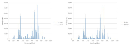
Figure 6.
Spectral emission from the sputtering plasma under various chamber pressures. Comparing chamber pressures of 2.1 mbar and 3.7 mbar (left) and comparing 1 mbar and 4.1 mbar chamber pressures (right). The objective is to have the model learn the spectral features of the plasma and predict the sheet resistance of the thin films of indium-doped zinc oxide thin films purely from these spectral features, without the need for delving into complex plasma physics models.
We undertook three approaches toward preparing and implementing the data to train our neural network models: (a) an ANN-based integral approach with 50 nm spectral windows, (b) an ANN-based spectral approach and (c) a CNN-ANN-based spectral approach that deviated into computer vision and image recognition, wherein we converted the spectral data into two-dimensional scaled images, implemented an advanced computer vision deep learning convolutional neural network as an image recognition model and coupled it to a neural network model for regression analysis (Figure 7).
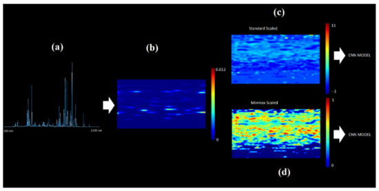
Figure 7.
Conversion of the spectral plot of the plasma into 2D images formed from scaling the spectral values. Images were generated from standard scaled and min-max scaled spectral data. The images were then fed into a convolutional neural network model coupling image recognition and regression analysis. (a) is the original spectra, (b) is an image directly formed from the original spectra, (c) is an image formed from the standard scaling of the original spectra, (d) is an image formed from the min max scaling of the original spectra.
3.2.1. The Integral Approach
The integral approach proceeded with calculating the area under the spectral peaks in 50 nm intervals from 300 to 900 nm, giving us a data frame with 12 columns associated with these areas. This resulted in a data frame with 517 rows and 12 columns associated with peak area values, while the 13th column was a vector of thin film sheet resistance values. Figure 8 presents the structure of the neural network model for the integral approach to model construction, as well as the predictions of the model for sheet resistance of 24 randomly selected samples. The optimizer for this model was Adam [54], with a learning rate of 0.01 and Huber loss function [55].
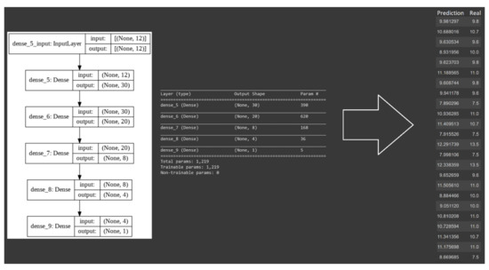
Figure 8.
The structure of the neural network model designed for training with the integral approach. The model is composed of five dense layers. Layers 1 to 5 have 30, 20, 8, 4 and 1 neuron/s, respectively, generating a total of 1219 parameters requiring computation. The model’s R2 value is 0.795.
We observed a total of 24 predictions of sheet resistance by the model, as compared to the actual sheet resistance measured via a Jandel four-point probe system. The R2 value for the models’ predictions was 0.795 with a mean squared error of 0.7.
However, rerunning the sample would demonstrate instability, which could be associated with the small size of the data frame. As discussed, neural network models require large datasets for training and our dataset, although large from a practical material engineering perspective, was comparatively small compared to standard datasets implemented in data science and machine learning.
3.2.2. The Spectral Approach
In the spectral approach, the objective was to use the peak intensity values across the spectrum from 195 to 1104 nm with a resolution of 0.2 nm. This approach would lead to a data frame composed of 113 rows and 4552 columns. All the negative values from the spectrometer signal (noise) were adjusted to 0. The columns of the data frame represented the ratio of the intensity of the spectral signal at each wavelength over the total sum of the intensity. The structure of the model and its predictions are presented in Figure 9.

Figure 9.
The structure of the neural network model designed for training with the spectral approach. The model is composed of eight dense layers. Layers 1 to 8 have 4551, 2000, 500, 300, 50, 8, 4 and 1 neuron/s, respectively, generating a total of over 30 million parameters requiring computation. The model’s R2 value is 0.153.
From the results presented in Figure 9, we can see that the model was significantly larger and more complex than the previous model handling integral data frame. The model had to handle over 30 million parameters compared to the 1219 parameters of the previous model, which was computationally very expensive. Nevertheless, the model’s statistical performance with R2 value of 0.15 was no match for the 0.795 R2 value of the previous model.
Various neural network structures were constructed to handle the spectral data frame system; the model reported here was the best performing model by far. We decided to implement principal component analysis (PCA) on our spectral data frame to reduce its large dimensionality [56]. This was a form of feature engineering. By implementing PCA, we reduced the number of feature columns from 4552 columns to only 12 columns. PCA extracted hidden factors from the dataset and defined data using a smaller number of components, which explained the variance in data. As such, it reduced the computational complexity. We then implemented these 12 principal components as the input for the neural model. The structure of the model and its predictions on physically measured samples are presented in Figure 10.

Figure 10.
The structure of the neural network model designed for training with the combined principal component analysis and spectral approach. The model is composed of seven dense layers. Layers 1 to 7 have 10, 10, 10, 10, 8, 4 and 1 neuron/s, generating a total of 349 parameters requiring computation; the model’s R2 value is 0.883.
As presented in Figure 10, in the PCA/spectral data frame integration approach, the model outperformed our integral approach experiment with an R2 value of 0.883—significantly better than the previous models.
3.2.3. The Image Recognition Approach
The spectral data collected between 200 to 1100 nm with a resolution of 0.2 nm created an array of 4500 data points. This array was converted into a matrix of shape (50, 90). This matrix was then converted into an image where each value of the matrix represented a pixel value of an 50 pixel × 90 pixel image. This is illustrated in Figure 11.
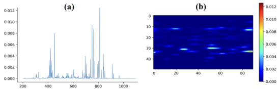
Figure 11.
Converting a spectral plot (a) into an image (b). The spectral data are initially summed up and each peak value is calculated by dividing the original peak value over the sum. It is then converted into a matrix of (50, 90) shape.
The image generated directly from the spectra was used to train various convolutional neural network models. However, none of the models were able to learn from the image in its direct form as CNN models work efficiently with standardised values. The image pixel values were then scaled using two different normalising methods: min-max scaling and standard scaling.
New images were generated from the normalised values of the pixels associated with the original image. Two examples are presented in Figure 12.
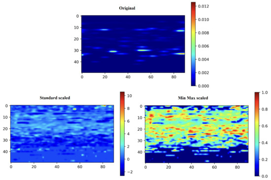
Figure 12.
The original image (top) is converted to an image from normalised values via standard scaling (bottom left) and min-max scaling methods (bottom right).
The normalised images were then used to train the model to predict the sheet resistances of the IZO films deposited via the associated plasma.
The normalised images were then tested via similar convolutional models. The results are presented in Figure 13 and Figure 14. Interestingly, the min-max scaled data resulted in best performance of sheet resistance prediction, as illustrated in the results and R2 values, with standard scaled images showing R2 values of 0.642 and min-max scaled images showing R2 values of 0.897.
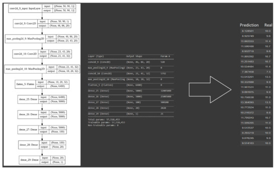
Figure 13.
The structure of the convolutional neural network model designed for training with standard scaled values of the pixels in image of the spectra. The model is composed of two convolutional layers and two max-pooling layers which are then flattened and fed to a deep network with five dense layers. Where layers 1 to 5 had 5000, 5000, 100, 20, and 1 neuron/s, generating a total of 57,518,453 parameters requiring computation, the model’s R2 value was 0.642.
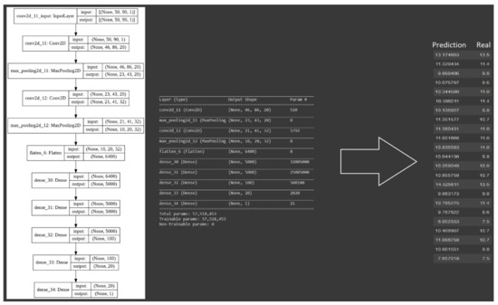
Figure 14.
The structure of the convolutional neural network model designed for training with the min-max scaled values of the pixels in images of the spectra. The model is composed of two convolutional layers and two max-pooling layers which are then flattened and fed to a deep network with five dense layers. Where layers 1 to 5 had 5000, 5000, 100, 20, and 1 neuron/s, generating a total of 57,518,453 parameters requiring computation, the model’s R2 value was 0.897.
The results so far indicated that min-max scaling of the data allowed the CNN model to perform more accurately on recognising the patterns and hidden features of the image.
In the next step, as each image was technically a matrix of size (50, 90), we applied singular value decomposition (SVD) to every single image. The SVD decomposed the image matrix into three matrices: a U matrix, which spanned the column space of the image; a V matrix, which spanned the row space of the image; and a diagonal matrix holding singular values that were scalers associated with consecutive columns of U and V. The whole image was able to be reconstructed from the out product of U and V scaled by the diagonal singular value matrix. This is illustrated in Figure 15.
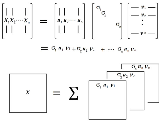
Figure 15.
The singular value decomposition and reconstruction of a matrix. Once a matrix is decomposed, it can be reconstructed back layer by layer, where each layer is formed via the outer product of the vectors spanning the column space of the original matric and vectors spanning the row space of the matrix and the associated singular value.
The vectors in U and V were unit vectors. The associated singular value acted as a scaler which gave the magnitude to the outer product of these vectors. The condition number of a matrix reflects the spread of information within a matrix and can be obtained by dividing the highest singular value of a matrix over its lowest singular value. In our results, although both standard scaled and min-max scaled image matrices demonstrated similar condition numbers, the spread of information associated with each singular value was different when we performed SVD on the images.
Figure 16 represents the (scree plot) typical spread of singular values for each layer of a decomposed standard scaled and min-max scaled matrix. In a min-max scaled matrix, the first singular value (the max value) held a higher percentage of the sum of all values compared to the standard scaled decomposed matrices.
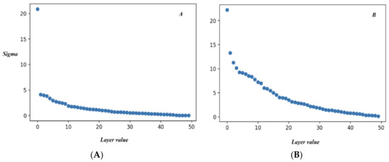
Figure 16.
The scree plot of singular values for (A) min-max scaled images and (B) standard scaled images.
In the next step of our efforts to increase the accuracy of the CNN model, we reconstructed the decomposed spectral image matrices layer by layer (from a total of 50 layers for each image) and trained the CNN model with images reconstructed from smaller layers—or even a single layer—of the SVD process. As the standard scaled whole images performed poorly before (see Figure 13, R2 value 0.642), we were seeking better performance from the min-max scaled values. However, to our surprise, an image reconstructed from the first single layer of the standard scaled images decomposed by SVD outperformed all our other CNN training efforts with an R2 value of 0.935. Most importantly, the model was the most stable in terms of its output on repeated trainings. Comparatively, reconstructing an image from the first single layer of a min-max scaled image performed very poorly in training the CNN model with R2 value of 0.74.
This observation was very intriguing for us. The standard scaled original images performed poorly in training the CNN model, while the min-max scaled original images performed very well. Meanwhile, the first single layer reconstruction of a standard scaled image outperformed all models in terms of accuracy and stability. Hence, as we carried out these experiments in a set of chamber pressures, we decided to convert the reconstructed images from the first layer of the singular value decomposed original images into a spectral format. These results are presented in Figure 17 and Figure 18. Each column in these figures represented four randomly selected spectral reconstructions of the plasma emissions from the first layer of the SVD of the original image, at a particular chamber pressure.
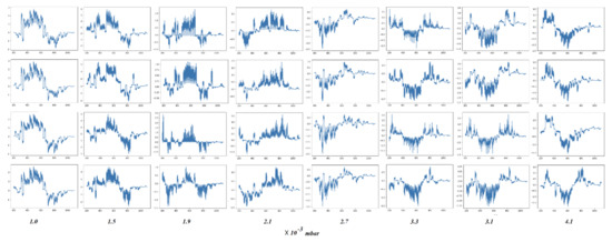
Figure 17.
Four randomly selected conversions of the first layer of the image decomposition via SVD, associated with process chamber pressures into a spectral format. For standard scaled images. x-axis represents emission wavelengths and y-axis is emission intensity. To the naked human eye, these patterns won’t mean much, however the deep learning model is able to pick up features beyond human vision.
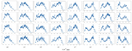
Figure 18.
Four randomly selected conversions of the first layer of the image decomposition via SVD associated with process chamber pressures into a spectral format. For min-max scaled images, x-axis represents emission wavelengths and y-axis is emission intensity.
The predictions of the CNN model from standard scaled image data are presented in Table 1.

Table 1.
Prediction of the thin film sheet resistance from a CNN model learning from the first layer of a singular value decomposed image of a plasma spectra (standard scaled).
The observed training performance associated with standard scaled first layer images may be explained by comparing images in Figure 17 and Figure 18. Convolutional neural networks essentially operate by identifying specific features in an image. These features (and their detection within the black box of a deep neural network) are not very intuitive and sometimes mysterious. As such, standard scaling of the images that were constructed from the original plasma spectrum formed features that were packed in a particular column and row space of the image, while the min-max scaling resulted in feature distribution across other row and column vector spaces. However, as our long-term approach was to explore the suitability of deep learning models for moving toward digitised sputtering processes, we accepted the model’s performance. Nonetheless, this is an interesting topic, to be pursued by researchers with a primary focus on the actual engineering of deep learning models.
The overall performances of all of our experiments, in terms of their predictive accuracy, are presented in Table 2.
Table 2.
The overall performance of the models and the data approach in our experiments. The R2 value is the highest achieved for the CNN model approach. The stability reflects how repeatable the model’s consecutive R2 values were, i.e., how they differed from the max R2 obtained. Poor indicates a deviation of 0.15 points, moderate indicates 0.1 and good indicates 0.05, when the models were repeated ten times.
4. Conclusions
Implementing deep learning models in spectral analyses of sputtering plasma has the potential to digitise the sputtering process, in the sense that, during the deposition a particular property of the film may be estimated purely from observing the characteristics of the plasma. Following different modelling approaches, as summarised in Table 2, the CNN model approach resulted in the highest R2 value with a good stability. The study showed that the accuracy of the results was dependent on the number of data points and number of process parameters considered. The accuracy also depended on the modelling approach followed. Certainly, our future attempts will involve explorations of other features of the samples, such as charge carrier concentration, mobility, crystal structure parameters and optical band gap. We also intend to vary other parameters of the experiment, such as sample rotation speed, incident angle of the magnetron to the substrate and their distance for predicting the functionality of the deposited films with a high degree of accuracy.
At the same time, expert researchers in the fields of data science, AI and machine learning are developing more and more accurate algorithms, loss functions, back propagation models and optimisations to further enhance this science as a tool available to all other areas of science. Surely, the models presented in this report could be fine-tuned further and further in order to achieve higher accuracies. As such, the process of digitised manufacturing in the field of thin film depositions could significantly benefit from integrating the process of the AI, as illustrated in our study and related to functional properties, like sheet resistance of a TCO film.
However, as discussed earlier, deep learning models require large datasets as input for the learning stage. Currently, academics in the fields of chemistry and material sciences conduct numerous experiments and generate significant data, collectively. However, most of these data remain unused or are discarded when the desirable outcome from the experiment is not achieved. For example, lead researchers working on thin film perovskite solar cells produce numerous devices within their research groups and tend to keep for further study only those samples which perform above a certain threshold. Even then, most of the data remain unstructured and unnoticed. Machine learning models learn from data, irrespective of the data being associated to a poor performance or an optimised device. Our research is currently supported via a GCRF/EPSRC-supported initiative holding multiple partner organisations from two countries (India and the UK), collaborating on the development of new generation and disruptive thin film solar cells for affordable electricity for villages in India. Many of our collaborators have conducted (or do conduct) sputter deposition of thin films; however, during our inquest, we realised that only data associated with desirable outcomes are stored or structured, while huge quantities of data that are generated at great expense over significant amounts of time are wasted.
In this paper, we noted the potential for further improvements in our model construction if we had more data (specifically from other sputter systems) which, unfortunately, were not available. However, our efforts within these limitations represented a step towards correlating digital datasets with the desired functionality of the TCO films with reasonable accuracy. Thus, this work will be of significance for optoelectronic industries using physical vapor deposition (sputtering, in this case) to realise a product with a high yield. Hence, in conclusion, we believe our results have suggested the necessity of the formation of a global repository, where data generated at each level of research by various research groups (such as material engineers, like us) will be made available for analysis and model training. Long term, this will reduce research and development costs and accelerate the development of novel materials and technologies—and will benefit industries as they move toward efficient and cost-effective scaling-up of their productions.
Author Contributions
Conceptualization, A.S.; Data curation, A.S. and A.A.; Formal analysis, A.S.; Investigation, A.S.; Methodology, A.S.; Resources, H.U.; Supervision, A.S.; Writing—original draft, A.S.; Writing—review and editing A.S. and H.U. All authors have read and agreed to the published version of the manuscript.
Funding
The authors deeply acknowledge the funding support from GCRF/EPSRC-supported SUNRISE program (EP/P032591/1).
Institutional Review Board Statement
Not applicable.
Informed Consent Statement
Not applicable.
Data Availability Statement
Data sharing is not applicable to this article.
Acknowledgments
H.U. would like to acknowledge the support received from industrial partner Scientific Vacuum Systems (SVS) Ltd. towards helping with sputtering equipment V6000-related maintenance and integration. We also thank Brunel University London for their support in providing access to the V6000 unit. We would like to dedicate this article to our loving friend, colleague and co-author, the late Arjang Aminishahsavarani, who unexpectedly passed away after submitting this article.

Conflicts of Interest
The authors declare no conflict of interest.
References
- Lewis, B.; Paine, D. Applications and Processing of Transparent Conducting Oxides. MRS Bull. 2000, 25, 22–27. [Google Scholar] [CrossRef]
- Crintea, D.; Czarnetzki, U.; Iordanova, S.; Koleva, I.; Luggenhölscher, D. Plasma diagnostics by optical emission spectroscopy on argon and comparison with Thomson scattering. J. Phys. D Appl. Phys. 2009, 42, 045208. [Google Scholar] [CrossRef]
- Zhu, X.; Pu, Y. Optical emission spectroscopy in low-temperature plasmas containing argon and nitrogen: Determination of the electron temperature and density by the line-ratio method. J. Phys. D Appl. Phys. 2010, 43, 403001. [Google Scholar] [CrossRef]
- Trevizan, L.; Santos, D.; Samad, R.; Vieira, N.; Nunes, L.; Rufini, I.; Krug, F. Evaluation of laser induced breakdown spectroscopy for the determination of micronutrients in plant materials. Spectrochim. Acta Part B At. Spectrosc. 2009, 64, 369–377. [Google Scholar] [CrossRef]
- Unnikrishnan, V.; Alti, K.; Nayak, R.; Bernard, R.; Khetarpal, N.; Kartha, V.; Santhosh, C.; Gupta, G.; Suri, B. Optimized LIBS setup with echelle spectrograph-ICCD system for multi-elemental analysis. J. Instrum. 2010, 5, P04005. [Google Scholar] [CrossRef]
- Bastiaans, G.; Mangold, R. The calculation of electron density and temperature in Ar spectroscopic plasmas from continuum and line spectra. Spectrochim. Acta Part B At. Spectrosc. 1985, 40, 885–892. [Google Scholar] [CrossRef]
- Iordanova, S.; Koleva, I. Optical emission spectroscopy diagnostics of inductively-driven plasmas in argon gas at low pressures. Spectrochim. Acta Part B At. Spectrosc. 2007, 62, 344–356. [Google Scholar] [CrossRef]
- Gurnett, D.A.; Bhattacharjee, A. Introduction to plasma physics: With space and laboratory applications. Choice Rev. Online 2005, 43, 43–0375. [Google Scholar]
- Montgomery, D.; Bellan, P.M. Fundamentals of plasma physics. Theor. Comput. Fluid Dyn. 2006, 21, 79–80. [Google Scholar] [CrossRef]
- Unnikrishnan, V.; Alti, K.; Kartha, V.; Santhosh, C.; Gupta, G.; Suri, B. Measurements of plasma temperature and electron density in laser-induced copper plasma by time-resolved spectroscopy of neutral atom and ion emissions. Pramana 2010, 74, 983–993. [Google Scholar] [CrossRef]
- Diwakar, P.; Hahn, D. Study of early laser-induced plasma dynamics: Transient electron density gradients via Thomson scattering and Stark Broadening, and the implications on laser-induced breakdown spectroscopy measurements. Spectrochim. Acta Part B At. Spectrosc. 2008, 63, 1038–1046. [Google Scholar] [CrossRef]
- Cadwell, L.; Hüwel, L. Time-resolved emission spectroscopy in laser-generated argon plasmas—Determination of Stark broadening parameters. J. Quant. Spectrosc. Radiat. Transf. 2004, 83, 579–598. [Google Scholar] [CrossRef]
- Shaikh, N.; Rashid, B.; Hafeez, S.; Jamil, Y.; Baig, M. Measurement of electron density and temperature of a laser-induced zinc plasma. J. Phys. D Appl. Phys. 2006, 39, 1384–1391. [Google Scholar] [CrossRef]
- Tawfik, W.; Askar, A. Study of the matrix effect on the plasma characterization of heavy elements in soil sediments using LIBS with a portable echelle spectrometer. Prog. Phys. 2007, 1, 46–52. [Google Scholar]
- Hong, Y.J.; Kwon, G.C.; Cho, G.; Shin, H.M.; Choi, E.H. Measurement of Electron Temperature and Density Using Stark Broadening of the Coaxial Focused Plasma for Extreme Ultraviolet Lithography. IEEE Trans. Plasma Sci. 2010, 38, 1111–1117. [Google Scholar] [CrossRef]
- Palmero, A.; van Hattum, E.; Arnoldbik, W.; Habraken, F. Argon plasma modelling in a RF magnetron sputtering system. Surf. Coat. Technol. 2004, 188–189, 392–398. [Google Scholar] [CrossRef]
- Christie, D.J. Target material pathways model for high power pulsed magnetron sputtering. J. Vac. Sci. Technol. A 2005, 23, 330–335. [Google Scholar] [CrossRef]
- Kolev, I. Particle-In-Cell-Monte-Carlo Collisions Simulations for a Direct Current Planar Magnetron Discharge. Ph.D. Thesis, University of Antwerp, Antwerp, Belgium, 2007. [Google Scholar]
- Brenning, N.; Huo, C.; Lundin, D.; Raadu, M.; Vitelaru, C.; Stancu, G.; Minea, T.; Helmersson, U. Understanding deposition rate loss in high power impulse magnetron sputtering: I. Ionization-driven electric fields. Plasma Sources Sci. Technol. 2012, 21, 025005. [Google Scholar] [CrossRef]
- Huo, C.; Raadu, M.; Lundin, D.; Gudmundsson, J.; Anders, A.; Brenning, N. Gas rarefaction and the time evolution of long high-power impulse magnetron sputtering pulses. Plasma Sources Sci. Technol. 2012, 21, 045004. [Google Scholar] [CrossRef]
- Shidoji, E.; Ohtake, H.; Nakano, N.; Makabe, T. Two-Dimensional Self-Consistent Simulation of a DC Magnetron Discharge. Jpn. J. Appl. Phys. 1999, 38, 2131–2136. [Google Scholar] [CrossRef]
- Kolev, I.; Bogaerts, A. Numerical Models of the Planar Magnetron Glow Discharges. Contrib. Plasma Phys. 2004, 44, 582–588. [Google Scholar] [CrossRef]
- Sheridan, T.; Goeckner, M.; Goree, J. Pressure dependence of ionization efficiency in sputtering magnetrons. Appl. Phys. Lett. 1990, 57, 2080–2082. [Google Scholar] [CrossRef][Green Version]
- Goeckner, M.; Goree, J.; Sheridan, T. Monte Carlo simulation of ions in a magnetron plasma. IEEE Trans. Plasma Sci. 1991, 19, 301–308. [Google Scholar] [CrossRef]
- Passoth, E.; Behnke, J.; Csambal, C.; Tichý, M.; Kudrna, P.; Golubovskii, Y.; Porokhova, I. Radial behaviour of the electron energy distribution function in the cylindrical magnetron discharge in argon. J. Phys. D Appl. Phys. 1999, 32, 2655–2665. [Google Scholar] [CrossRef]
- Porokhova, I.; Golubovskii, Y.; Bretagne, J.; Tichy, M.; Behnke, J. Kinetic simulation model of magnetron discharges. Phys. Rev. E 2001, 63, 056408. [Google Scholar] [CrossRef]
- Porokhova, I.; Golubovskii, Y.; Behnke, J. Anisotropy of the electron component in a cylindrical magnetron discharge. I. Theory of the multiterm analysis. Phys. Rev. E 2005, 71, 066406. [Google Scholar] [CrossRef]
- Porokhova, I.; Golubovskii, Y.; Behnke, J. Anisotropy of the electron component in a cylindrical magnetron discharge. II. Application to real magnetron discharge. Phys. Rev. E 2005, 71, 066407. [Google Scholar] [CrossRef]
- Birdsall, C. Particle-in-cell charged-particle simulations, plus Monte Carlo collisions with neutral atoms, PIC-MCC. IEEE Trans. Plasma Sci. 1991, 19, 65–85. [Google Scholar] [CrossRef]
- Revel, A.; Minea, T.; Costin, C. 2D PIC-MCC simulations of magnetron plasma in HiPIMS regime with external circuit. Plasma Sources Sci. Technol. 2018, 27, 105009. [Google Scholar] [CrossRef]
- Tozer, B. Rotating plasma. Proc. Inst. Electr. Eng. 1965, 112, 218. [Google Scholar] [CrossRef]
- Wasa, K.; Hayakawa, S. Formation of Rotating Plasma in Crossed Field. J. Phys. Soc. Jpn. 1966, 21, 738–743. [Google Scholar] [CrossRef]
- Wilcox, J.; Cooper, W.; DeSilva, A.; Spillman, G.; Boley, F. Swirls Produced in a “Crowbarred” Rotating Plasma. J. Appl. Phys. 1962, 33, 2714–2715. [Google Scholar] [CrossRef][Green Version]
- Anders, A. Localized heating of electrons in ionization zones: Going beyond the Penning-Thornton paradigm in magnetron sputtering. Appl. Phys. Lett. 2014, 105, 244104. [Google Scholar] [CrossRef]
- Panjan, M.; Loquai, S.; Klemberg-Sapieha, J.; Martinu, L. Non-uniform plasma distribution in dc magnetron sputtering: Origin, shape and structuring of spokes. Plasma Sources Sci. Technol. 2015, 24, 065010. [Google Scholar] [CrossRef]
- Anders, A.; Yang, Y. Direct observation of spoke evolution in magnetron sputtering. Appl. Phys. Lett. 2017, 111, 064103. [Google Scholar]
- Anders, A.; Yang, Y. Plasma studies of a linear magnetron operating in the range from DC to HiPIMS. J. Appl. Phys. 2018, 123, 043302. [Google Scholar] [CrossRef]
- Andersson, J.; Ni, P.; Anders, A. Smoothing of Discharge Inhomogeneities at High Currents in Gasless High Power Impulse Magnetron Sputtering. IEEE Trans. Plasma Sci. 2014, 42, 2856–2857. [Google Scholar]
- Arcos, T.; Layes, V.; Gonzalvo, Y.; Gathen, V.; Hecimovic, A.; Winter, J. Current–voltage characteristics and fast imaging of HPPMS plasmas: Transition from self-organized to homogeneous plasma regimes. J. Phys. D Appl. Phys. 2013, 46, 335201. [Google Scholar]
- Šlapanská, M.; Hecimovic, A.; Gudmundsson, J.; Hnilica, J.; Breilmann, W.; Vašina, P.; von Keudell, A. Study of the transition from self-organised to homogeneous plasma distribution in chromium HiPIMS discharge. J. Phys. D Appl. Phys. 2020, 53, 155201. [Google Scholar]
- Hecimovic, A.; Corbella, C.; Maszl, C.; Breilmann, W.; von Keudell, A. Investigation of plasma spokes in reactive high power impulse magnetron sputtering discharge. J. Appl. Phys. 2017, 121, 171915. [Google Scholar] [CrossRef]
- Depla, D.; Mahieu, S. Reactive Sputter Deposition; Springer Series in Materials Science; Springer: Berlin/Heidelberg, Germany, 2008; Volume 109. [Google Scholar]
- Marcak, A.; Corbella, C.; de los Arcos, T.; von Keudell, A. Note: Ion-induced secondary electron emission from oxidized metal surfaces measured in a particle beam reactor. Rev. Sci. Instrum. 2015, 86, 106102. [Google Scholar] [CrossRef] [PubMed]
- Yang, Y.; Zhou, X.; Liu, J.; Anders, A. Evidence for breathing modes in direct current, pulsed, and high power impulse magnetron sputtering plasmas. Appl. Phys. Lett. 2016, 108, 034101. [Google Scholar] [CrossRef]
- Yang, Y.; Tanaka, K.; Liu, J.; Anders, A. Ion energies in high power impulse magnetron sputtering with and without localized ionization zones. Appl. Phys. Lett. 2015, 106, 124102. [Google Scholar] [CrossRef]
- Anders, A.; Ni, P.; Andersson, J. Drifting Ionization Zone in DC Magnetron Sputtering Discharges at Very Low Currents. IEEE Trans. Plasma Sci. 2014, 42, 2578–2579. [Google Scholar] [CrossRef]
- Held, J.; Maaß, P.; Gathen, V.; Keudell, A. Electron density, temperature and the potential structure of spokes in HiPIMS. Plasma Sources Sci. Technol. 2020, 29, 025006. [Google Scholar] [CrossRef]
- Schmidhuber, J. Deep learning in neural networks: An overview. Neural Netw. 2015, 61, 85–117. [Google Scholar] [CrossRef]
- Hinton, G.; Rumelhart, D. Neural Network Architectures for Artificial Intelligence; American Society for Artificial Intelligence: San Mateo, CA, USA, 1988. [Google Scholar]
- Introduction to Convolutional Neural Networks. 2017. Available online: https://cs.nju.edu.cn/wujx/paper/CNN.pdf (accessed on 22 November 2021).
- Lecun, Y. Gradient Based Learning for Document Recognition. 1998. Available online: http://yann.lecun.com/exdb/publis/pdf/lecun-01a.pdf (accessed on 22 November 2021).
- He, K.; Zhang, X.; Ren, S.; Sun, J. Spatial Pyramid Pooling in Deep Convolutional Networks for Visual Recognition. IEEE Trans. Pattern Anal. Mach. Intell. 2015, 37, 1904–1916. [Google Scholar] [CrossRef]
- Suárez-Paniagua, V.; Segura-Bedmar, I. Evaluation of pooling operations in convolutional architectures for drug-drug interaction extraction. BMC Bioinform. 2018, 19, 39–47. [Google Scholar] [CrossRef]
- Aparnev, A.; Barten’ev, O. Analyzing the Loss Functions in Training Convolutional Neural Networks with the Adam Optimizer for Classification of Imagess. Vestn. MEI 2020, 2, 90–105. [Google Scholar] [CrossRef]
- Balasundaram, S.; Prasad, S. Robust twin support vector regression based on Huber loss function. Neural Comput. Appl. 2019, 32, 11285–11309. [Google Scholar] [CrossRef]
- Beattie, J.; Esmonde-White, F. Exploration of Principal Component Analysis: Deriving Principal Component Analysis Visually Using Spectra. Appl. Spectrosc. 2021, 75, 361–375. [Google Scholar] [CrossRef] [PubMed]
Publisher’s Note: MDPI stays neutral with regard to jurisdictional claims in published maps and institutional affiliations. |
© 2022 by the authors. Licensee MDPI, Basel, Switzerland. This article is an open access article distributed under the terms and conditions of the Creative Commons Attribution (CC BY) license (https://creativecommons.org/licenses/by/4.0/).