A New Strong Form Technique for Thermo-Electro-Mechanical Behaviors of Piezoelectric Solids

Abstract

Piezoelectric materials are widely fabricated and investigated for potential applications in microelectromechanical systems as direct converters between mechanical and electrical signals, where some show pyroelectric features involving thermo-electro-mechanical interactions. This study aimed to introduce a novel numerical technique to predict the thermo-electro-mechanical behaviors of piezoelectric structures, based on a strong-form numerical framework called the element differential method. In this method, the shape functions of the isoparametric element and their first two derivatives were derived analytically by interpolating the temperature, displacement, and electric potentials. Then, a point collocation method based on node positions in the elements was proposed to generate the final system of equations without any domain integrations. Thus, the coupled behaviors of thermal piezoelectric structures, including the pyroelectric features, can be simulated by the strong-form formulation of the governing equations. Several numerical examples, including the piezoelectric composites structures, are presented, and the coupled thermo-electro-mechanical responses have been analyzed to validate the proposed method.

1. Introduction

With the fast development of smart materials and manufacturing technologies, the thermo-electro-mechanical coupled responses of the smart structures have attracted instant attention from scientists. P piezoelectric materials have been broadly employed as actuators or sensors depending on the coupled mechanical and electrical characteristics. These devices can provide high-level features such as high force generation, response speed, and displacement accuracy [1,2]. Moreover, because thermo-piezoelectric materials possess the potential capability in aviation, transportation, and automating industries [3], they have been also widely selected in designing the devices for damage detecting, health inspecting, actuating, and load-carrying applications [4,5]. For instance, research indicates that the sensing devices based on pyroelectric and piezoelectric effects have potential applications in the design of active human-computer interaction and wearable robots [6,7].

The smart piezoelectric devices composed of thermo-electro-elastic properties often run at the different loading environments, such as cyclic electrical or mechanical, thermal, and or their combined conditions. In literature, a significant amount of research focuses on simulating and investigating the coupling structural responses of piezoelectric materials. Completely understanding the coupling behaviors or the physical laws will be beneficial in utilizing the thermo-piezoelectric materials in real engineering applications. The research [8,9] demonstrated that the polarization of the crystalline materials and structures could be affected by the temperature. Due to the temperature changes, the piezoelectric material may be polarized by establishing the electrical potentials [10].

On the other hand, a complete understanding of thermal stress is necessary to guarantee the reliabilities of piezoelectric structures in real applications, such as the aerospace industry, especially when piezoelectric structures are exposed to complex and changeable temperature environments [11,12]. Namli and Taya introduced a thermal energy piezo-SMA harvester subjected to temperature fluctuation in different frequencies [13]. Srivastava et al. designed a device to directly convert heat to electricity, in which energy conversion devices are designed according to the distributions of the electro-thermo-elastic coupling fields [14]. In addition, thermal effect analyses of the thermal piezoelectric structures could provide a theoretical basis of piezoelectric materials to predict the crack failure behaviors [15]. Consequently, the accurate analysis of the thermo-electro-mechanical behaviors of the piezoelectric materials under thermal environments is of great importance to understand the mechanism of interaction among different physical fields.

In this regard, recent literature has concentrated on developing novel numerical methods to analyze the multi-field coupling problems of the piezoelectric structures subjected to electrical, mechanical, and thermal loadings. Several illustrative numerical methods have been developed to analyze the thermo-electro-mechanical responses of piezoelectric structures, such as the finite element methods (FEM), the finite difference method (FDM), and the boundary element methods (BEM). Among them, the FEM is one of the most convenient computational tools. It has been widely utilized to calculate the boundary value problems of the piezoelectric medium subjected to complex loading conditions. For instance, the finite element formulation has been utilized to solve the crack problems under thermal loadings for piezoelectric structures with different size scales [16]. Rahman used FEM to analyze the free vibration analysis and steady harmonic analysis of a multilayer porous cantilever beam with a piezoelectric layer [17]. Jiang and Li introduced a finite element formulation to compute the energy harvesting problems of the piezoelectric composite beams under thermo-electro-mechanical loadings [18]. Amini et al. selected the FEM to calculate the coupled response of the piezoelectric harvesters made of functional graded materials in unimorph or bimorph arrangement [19].

Meanwhile, Yan and Jiang studied the dynamic fracture behaviors of piezoelectric materials based on the same numerical method [20]. The standard FEM to simulate the coupled problems of piezoelectric structures has been widely integrated into some of the commercial finite element codes, such as ABAQUS and ANSYS [21]. Although the overall success has been achieved through the finite element method to analyze piezoelectric problems, to the best of the authors’ knowledge, even some of the commercial finite element codes still cannot simulate the pyroelectric behaviors directly due to the complexity of the problems. Therefore, it will be interesting to study the pyroelectric properties of piezoelectric cellular structures with more convenient methods. For instance, Lv et al. introduced an extended multiscale finite element method for thermoelectric coupling responses of piezoelectric structures with pyroelectric effects [22].

The numerical methods derived from strong formulations to calculate piezoelectric behaviors have received growing interest in recent years. Generally, the solutions based on the strong-form technique can directly generate the system of equations without any other supplementary methods [23,24]. Thus, the strong-form method shows unrivaled favorable circumstances to simulate complex engineering problems, especially for multiphysics problems with different governing equations [25]. For instance, Moradi-Dastjerdi et al. used a meshless method to investigate the damped dynamic motions of piezoelectric sandwich plates under thermo-electromechanical loads [26]. Liew proposed a Galerkin differential quadrature method (DQM) to simulate the nonlinear behaviors of the thermo-piezoelectric structures [27]. Alashti and Khorsand also proposed a DQM to calculate the three-dimensional thermo-elastic problems of the cylindrical shells composed of piezoelectric layers under the thermo-electro-mechanical loads [28]. Recently, Lv et al. presented a type of strong form method to predict response of piezoelectric structures [29]. Their research indicated that the element differential method derived from the strong-form technique combines the benefits of standard FEMs, i.e., mesh grids can be generated adaptively for arbitrary configurations in real applications. At the same time, the strong form of governing equations can be directly utilized.

In this work, the research focused on the strong-form techniques to simulate the coupled responses of thermo-piezoelectric structures. A novel strong-form collocation method is presented to solve the coupled thermo-piezoelectric-mechanical behaviors. The isoparametric elements were introduced to assemble the governing partial differential equations of coupling problems. Then, according to the distributions of the nodes, a special collocation technique is used to construct the system equations for the coupled problems directly. The uncoupled procedure based on the standard Fourier heat conduction theory is utilized for thermo-electro-elastic behaviors. Furthermore, an additional innovation of the present strong-form method is that the pyroelectric effects of the piezoelectric structure are directly substituted into the system of equations through the collocation technique without any domain integrations. Finally, serval illustrative examples, including the complex piezoelectric composite structures, are proposed to validate the accuracy of the current method.

This paper’s remaining is organized in the following manner: The main equations, including the governing equations and constitutive equations, are briefly introduced for the linear thermo-electro-elastic problems in Section 2. Section 3 presents the element differential formulations and the point collocation technique to construct the system equations to analyze the piezoelectric structures subjected to the thermo-electro-elastic loadings. The point collocation technique is separately introduced for the two types of problems. Section 4 gives some numerical examples for the code validation. The last section gives a summary and conclusions.

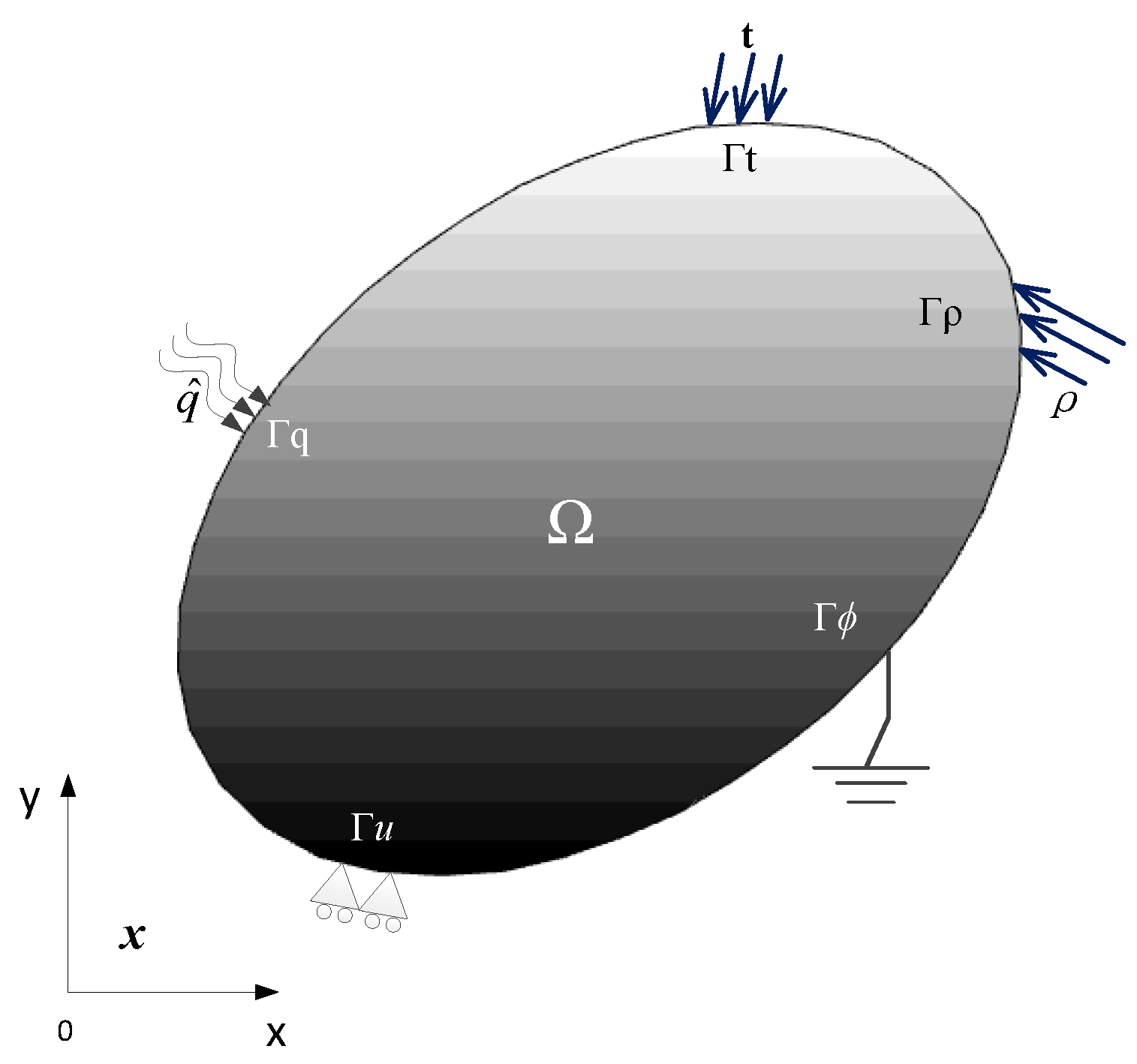
2. Unified Governing Equations for Thermo-Electro-Mechanical Problems

As indicated in Figure 1, a linear isotropic homogeneous piezoelectric domain subjected to the thermo-electro-mechanical loadings is considered. In this domain, the mechanical boundary conditions and prescribed electrical potentials are applied to the boundaries ${\mathsf{\Gamma }}_u$, ${\mathsf{\Gamma }}_{\varphi }$, respectively. At the same time, the traction t and the heat flux q act on boundaries ${\mathsf{\Gamma }}_t$, ${\mathsf{\Gamma }}_q$, respectively.

The constitutive equations for thermo-electro-mechanical problems can be written as [22]:

$$\begin{array}{l}{\sigma }_{ij}\left(\mathit{x}\right)=C_{ijkl}\left(\mathit{x}\right){\epsilon }_{kl}\left(\mathit{x}\right)+e_{mij}\left(\mathit{x}\right)\left(-E_m\left(\mathit{x}\right)\right)-{\beta }_{ij}T,\hfill \\ D_i\left(\mathit{x}\right)=e_{ijk}\left(\mathit{x}\right){\epsilon }_{jk}\left(\mathit{x}\right)-{\lambda }_{ik}\left(\mathit{x}\right)\left(-E_k\left(\mathit{x}\right)\right)-{\chi }_{i}T\hfill \end{array}$$

(1)

where ${\sigma }_{ij}$ are the stress tensors, ${\epsilon }_{kl}$ strain tensors, $D_i$ electric displacement vectors, $E_m$ electric field vectors, $C_{ijkl}$ elastic coefficient vectors, $e_{mij}$ piezoelectric stress coefficient vectors, ${\lambda }_{ik}$ dielectric coefficient vectors, ${\beta }_{ij}$ thermal-stress coefficient vectors and ${\chi }_i$ pyroelectric coefficient vectors, T the temperature variations. In two-dimensional problems, the ranges for the repeated subscripts i and j are 2, while in three-dimensional problems, the ranges are 3.

The parameters used in Equation (1) for three dimensional problems can be written in a unified way to simplify the expression of the constitutive equations for the thermo-piezoelectric materials

$$U_M=\{\begin{array}{c} u_m M=m=1,2,3\\ \varphi M=4 \end{array}, F_M=\{\begin{array}{c} f_m M=m=1,2,3\\ -q M=4 \end{array},$$

(2a)

$${\mathsf{\epsilon }}_{Mn}=\{\begin{array}{c} {\epsilon }_{mn} M=m=1,2,3\\ -E_n M=4 \end{array},{ \mathsf{\sigma }}_{Mn}=\{\begin{array}{c} {\sigma }_{mn} M=m=1,2,3\\ D_n M=4 \end{array}$$

(2b)

In the thermo-piezoelectric materials, the constitutive equations can be rewritten in an extended form

$${\sigma }_{Ij}=L_{IjMn}{\epsilon }_{Mn}+{\mathsf{\pi }}_{Ij}T$$

(3)

In Equation (3), $L_{IjMn}$ and ${\mathsf{\pi }}_{Ij}$ denote the constitutive coefficient matrixes, which can be written as

$$L_{IjMn}=\{\begin{array}{ll}{C}_{ijmn}\hfill & I=1,2,3,M=1,2,3\hfill \\ e_{nij}\hfill & I=1,2,3,M=4\hfill \\ e_{jmn}\hfill & I=4,M=1,2,3\hfill \\ -{\lambda }_{jn}\hfill & I=M=4\hfill \end{array}.$$

(4a)

$${\mathsf{\pi }}_{Ij}=\{\begin{array}{c}-{\beta }_{ij} I=1,2,3\\ -{\chi }_i I=4 \end{array}$$

(4b)

where, the ranges of the subscripts $I$ and M is 3 for 2D and 4 for 3D problems. With the symbolic forms presented above, the prescribed boundary conditions in the mechanical and electrical fields of the piezoelectric structures can be rewritten as:

$$U_M\left(x\right)={\overline{U}}_i\left(x\right),x\in {\mathsf{\Gamma }}_U,$$

(5a)

$${ℒ}_M\left(x\right)={\sigma }_{Mn}\left(x\right){\mathit{n}}_n-{\mathsf{\pi }}_{Mn}\left(x\right)T\left(x\right){\mathit{n}}_n={\overline{ℒ}}_M\left(x\right), \mathrm{on} {\mathsf{\Gamma }}_{ℒ}$$

(5b)

where ${\overline{U}}_i\left(x\right)$ denotes the fixed displacement and electrical potential values applied at the boundary ${\mathsf{\Gamma }}_{ℒ}$, the character ${\overline{ℒ}}_M$ denotes the unified form about the traction vectors and surface charges. The outward normal vector ${\mathit{n}}_n$ refers to the boundaries ${\mathsf{\Gamma }}_{ℒ}$. All the boundaries of the problem satisfy ${\mathsf{\Gamma }}_U={\mathsf{\Gamma }}_u{{\displaystyle \cup }}^{ }{\mathsf{\Gamma }}_{\varphi }, {\mathsf{\Gamma }}_{ℒ}={\mathsf{\Gamma }}_t{{\displaystyle \cup }}^{ }{\mathsf{\Gamma }}_D$.

Therefore, based on the extended form of the parameters, the obtained second-order partial differential equations of the thermal piezoelectric structure can be written as:

$$\frac{\partial L_{IjKl}}{\partial x_j}\frac{\partial U_K}{\partial x_l}+L_{IjKl}\frac{{\partial }^2{U}_K}{\partial x_l\partial x_J}+\frac{\partial \left({\mathsf{\pi }}_{Ij}T\right)}{\partial x_j}+F_I=0.$$

(6a)

where $F_I$ denotes the body force. At the same time, the boundary conditions related to the tractions and surface charges can be expressed as

$$L_{LiMn}\left(x\right){\mathit{n}}_n\frac{\partial U_L}{\partial x_i}-{\mathsf{\pi }}_{Mn}\left(x\right)T\left(x\right){\mathit{n}}_n={\overline{ℒ}}_M\left(x\right), \mathrm{on} {\mathsf{\Gamma }}_{ℒ}$$

(6b)

On the other hand, for the thermal conduction problems of the piezoelectric structure, the governing equation about the steady-state heat conduction response can be written as

$$\frac{\partial }{\partial x_i}\left(k_{ij}\left(\mathit{x}\right)\frac{\partial T}{\partial x_i}\right)+Q\left(\mathit{x}\right)=0$$

(7)

where, $k_{ij}\left(\mathit{x}\right)$ is the heat conductivity varying with coordinates x, Q(x) is the heat generated rate. Three types of boundary conditions can be generally considered to solve heat transfer problems of the piezoelectric solids

$$T\left(\mathit{x}\right)=\overline{T}\mathit{x}\in {\mathsf{\Gamma }}_1$$

(8)

$$q\left(\mathit{x}\right)=-k_{ij}\left(\mathit{x}\right)\frac{\partial T\left(\mathit{x}\right)}{\partial x_j}{\mathit{n}}_i=\overline{q}\mathit{x}\in {\mathsf{\Gamma }}_2$$

(9)

$$q\left(\mathit{x}\right)=-k_{ij}\left(\mathit{x}\right)\frac{\partial T\left(\mathit{x}\right)}{\partial x_j}{n}_i=h\left(T\left(\mathit{x}\right)-T_{\infty }\right) \mathit{x}\in {\mathsf{\Gamma }}_3$$

(10)

where ${\mathsf{\Gamma }}_1{{\displaystyle \cup }}^{ }{\mathsf{\Gamma }}_2{{\displaystyle \cup }}^{ }{\mathsf{\Gamma }}_3=\mathsf{\Gamma }$, $T\left(x\right)$ and $\overline{T}$ are the temperature and prescribed values, respectively. $\overline{q}$ is the specified heat flux. $T_{\infty }$ is the temperature on the boundary ${\mathsf{\Gamma }}_3$. h denotes the heat transfer coefficients.

3. Elemental Differential Method for Thermo-Electro-Mechanical Problems

In this section, a novel strong-form method called the thermal piezoelectric elemental differential method (TP-EDM) is introduced to analyze the coupled responses of the structures under thermo-electro-mechanical loadings. The proposed method can be divided into three steps. In the first step, target domains are discretized into isoparametric elements, consistent with those standard finite element methods. In the second step, the final system of equations is generated by the point collocation method. These equations are generated node by node in this step, while domain integrations element by element construct the total stiffness matrix. In the final step, the final system of the equation is solved to calculate the unknowns, i.e., nodal displacements, electrical potentials, and temperatures.

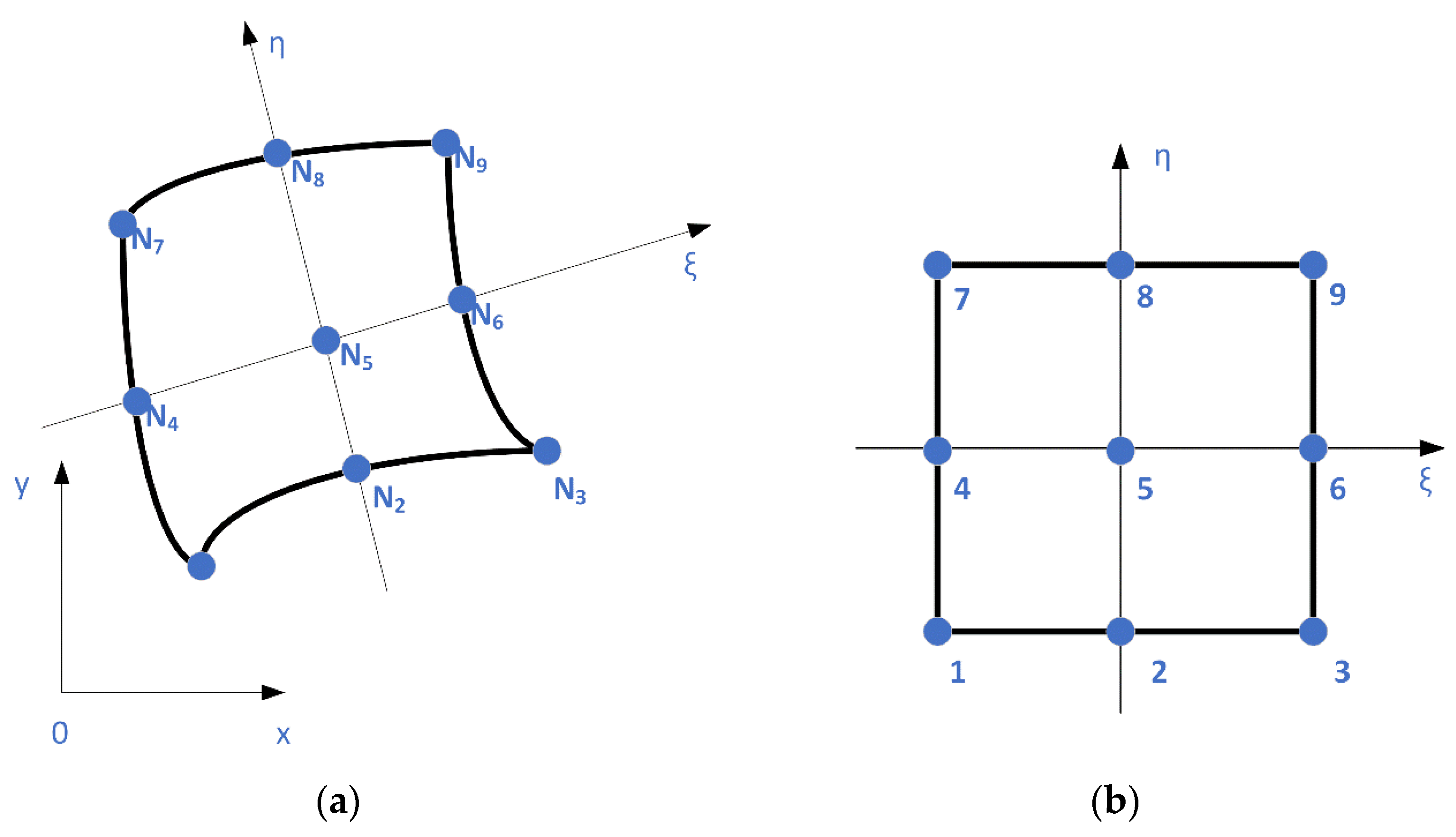
3.1. Lagrange Isoparametric Elements

The standard C0-continuous 2D and 3D Lagrange isoparametric elements are used to discretize the computation domain [25]. As illustrated in Figure 2, a 2D quadrilateral element with nine nodes is considered here. The main characteristic of the elements is that an independent node is distributed inside the elements. Based on the isoparametric element, the geometrical and physical variables over the element can be approximated according to the nodal values of the element.

Therefore, spatial coordinates, displacement, electrical potential, and temperature within an element can be calculated with the interpolation functions by

$$\{\begin{array}{c}{u}_i=N_{\alpha }\left(\mathit{\xi },\eta ,\zeta \right)u_i^{\alpha }\\ x_i=N_{\alpha }\left(\mathit{\xi },\eta ,\zeta \right)x_i^{\alpha }\\ \varphi =N_{\alpha }\left(\mathit{\xi },\eta ,\zeta \right){\varphi }_i^{\alpha }\\ T=N_{\alpha }\left(\mathit{\xi },\eta ,\zeta \right)T_i^{\alpha }\end{array}$$

(11)

where, $N_{\alpha }$ denotes the shape functions. The subscript $\alpha$ denotes the summation ranged from 1 to the number of the elemental nodes. It can be found that the mesh grids used in the standard finite element method can be directly employed for the computations of the current method.

The shape functions $N_{\alpha }$ for the isoparametric elements can be explicitly derived with the intrinsic coordinates [25]. In this regard, the first two orders of the partial differential equations for the shape functions referring to the spatial coordinates can be derived explicitly. The transformations of the derivatives can be written as follows:

$$\frac{\partial N_{\alpha }}{\partial x_i}=\frac{\partial N_{\alpha }}{\partial {\mathit{\xi }}_k}\frac{\partial {\mathit{\xi }}_k}{\partial x_i}={[J]}_{ik}^{-1}\frac{\partial N_{\alpha }}{\partial {\mathit{\xi }}_k},$$

(12)

$$\frac{{\partial }^2{N}_{\alpha }}{\partial x_i\partial x_j}=\left[{[J]}_{ik}^{-1}\frac{{\partial }^2{N}_{\alpha }}{\partial {\mathit{\xi }}_k\partial {\mathit{\xi }}_l}+\frac{\partial {[J]}_{ik}^{-1}}{\partial {\mathit{\xi }}_l}\frac{\partial N_{\alpha }}{\partial {\mathit{\xi }}_k}\right]\frac{\partial {\mathit{\xi }}_l}{\partial x_j}$$

(13)

where, the Jacobian matrix J denotes the mapping relationship between the Cartesian coordinate and the intrinsic coordinate systems. Based on the analytical expansion of the shape functions, the Jacobian matrix, its inverse matrix ${[J]}_{ik}^{-1}$ and derivative matrixes $\frac{\partial {[J]}_{ik}^{-1}}{\partial {\mathit{\xi }}_l}$ can be derived analytically, respectively [25].

3.2. Point Collocation Technique

This work assumes that the temperature distributions over the piezoelectric structures are independent of the electrical and elastic fields. The heat transfer problem is firstly calculated without considering the effects of the mechanical fields. Then the thermo-stress and the pyroelectric features of the piezoelectric structures are solved based on the obtained thermal fields. Although two different types of governing equations govern the two types of problems, the system equations of these boundary value problems can be constructed by the collocation technique in a unified way.

3.2.1. Point Collocation Technique for Thermal Conductions

As shown in Figure 3, the element nodes in the structures meshed with isoparametric elements can be clarified into three types according to their distributions, i.e., internal nodes located within the elements, interface nodes between elements, and outer surface nodes along boundaries.

For internal nodes located within an element, the set of equations can be directly created by governing equations of the thermal conduction problems. By combining Equations (7) and (12), the governing equations are expressed by the nodal element values of temperature [30]

$$\left[\frac{\partial N_{\beta }\left(\mathit{\xi }\right)}{\partial x_i}{k}_{ij}^{\beta }\frac{\partial N_{\alpha }\left(\mathit{\xi }\right)}{\partial x_j}+k_{ij}\left(\mathit{\xi }\right)\frac{{\partial }^2{N}_{\alpha }\left(\mathit{\xi }\right)}{\partial x_i\partial x_j}\right]T^{\alpha }+Q\left(\mathit{\xi }\right)=0$$

(14)

In the above equation, $\mathit{\xi }$ represents the intrinsic coordinates of the nodes, $k_{ij}^{\beta }$ the value of $k_{ij}$ at node $\beta$.

On the other hand, the heat flux should satisfy the equilibrium conditions at the other nodes distributed at element boundaries or interfaces shared by several elements. The equilibrium equations of the heat flux can be written as follows:

$${\displaystyle \sum }_{f=1}^M{q}_i^f\left(\mathit{x}\right)=\{\begin{array}{c}0, \mathrm{interface} \mathrm{nodes}\\ \overline{q_i}, \mathrm{boundary} \mathrm{nodes}\end{array}$$

(15)

where M denotes the quantity of element surfaces related to the interface nodes. $q_i^f\left(\mathit{x}\right)$ is the heat flux of surface f; $\overline{q_i}$ is the prescribed value of the heat flux.

For the nodes shared by several elements, the relationship between heat flux and temperature gradients can be obtained by substituting Equation (9) into Equation (14)

$${\displaystyle \sum }_{f=1}^K-k_{ij}\left({\mathit{\xi }}^I\right)\frac{{\partial }^2{N}_{\alpha }\left({\mathit{\xi }}^I\right)}{\partial x_j}{n}_i^f\left({\mathit{\xi }}^I\right)T^{\alpha }=0$$

(16)

where ${\mathit{\xi }}^I$ is the intrinsic coordinates of the interface nodes; $n_i^f$ is the outward normal vector to surface f.

On the other hand, for the nodes on the outer boundaries of mesh grids, the heat flux equilibrium conditions should be satisfied [30]

$${\displaystyle \sum }_{f=1}^K-k_{ij}\left({\mathit{\xi }}^b\right)\frac{{\partial }^2{N}_{\alpha }\left({\mathit{\xi }}^b\right)}{\partial x_j}{n}_i^f\left({\mathit{\xi }}^b\right)T^{\alpha }=q\left({\mathit{\xi }}^b\right)$$

(17)

where, ${\mathit{\xi }}^b$ is the intrinsic coordinates of the outer boundary nodes, $q\left({\mathit{\xi }}^b\right)=\overline{q}$ at the boundary ${\mathsf{\Gamma }}_2$, and $q\left({\mathit{\xi }}^b\right)=h\left(T\left({\mathit{\xi }}^b\right)-T_{\infty }\right)$ at the boundary ${\mathsf{\Gamma }}_3$.

3.2.2. Point Collocation Techniques for the Thermal Elastic Problems

A similar way can generate the system of equations for the thermal elastic response of the thermal piezoelectric structure as those for heat transfer problems. The governing equations for the thermal stress problems should be satisfied at all nodes inside elements

$$\left[L_{IjKl}\left(\mathit{\xi }\right)\frac{{\partial }^2{N}_{\alpha }\left(\mathit{\xi }\right)}{\partial x_j\partial x_l}+\frac{\partial N_{\beta }\left(\mathit{\xi }\right)}{\partial x_j}{L}_{jkl}^{\beta }\frac{\partial N_{\alpha }\left(\mathit{\xi }\right)}{\partial x_l}\right]U_K^{\alpha }+\frac{\partial \left({\mathsf{\pi }}_{Ij}\left(\mathit{\xi }\right)T\right)}{\partial x_j}+F_I\left(\mathit{\xi }\right)=0$$

(18)

where, $\mathit{\xi }$ denotes intrinsic coordinates of the node. The thermal-stress coefficients ${\mathsf{\pi }}_{Ij}$ can be directly considered in the governing equation. In this method the temperature difference is directly utilized in the governing equations to create the system of equations. Thus, the complexity in dealing with the thermal coupling problems of the piezoelectric structures can be greatly reduced.

For the other nodes, traction equilibrium conditions should be satisfied.

$${\displaystyle \sum }_{e=1}^{N^{}}{\displaystyle \sum }_{s=1}^{S^e}{ℒ}_i^s\left({\mathit{\xi }}^e\right)=\mathit{Q}=\{\begin{array}{cc}0,& \mathrm{internal} \mathrm{nodes}\hfill \\ {\displaystyle {\displaystyle \sum }_{e=1}^{N^{}}}{\displaystyle {\displaystyle \sum }_{s=1}^{S^e}}{\overline{ℒ}}_i^s,& \mathrm{boundary} \mathrm{nodes}\hfill \end{array}$$

(19)

In above equation, N represents the quantity of elements that includes the node considered, $S^e$ the quantity of surfaces of the element related to the node, $\overline{{ℒ}_i}\left(\mathit{x}\right)$ the surface tractions and charges applied.

Therefore, when the nodes are located at the element interfaces, the tractions for all the faces related to the considered nodes should be at an equilibrium state. The equation can be written as follows:

$${\displaystyle \sum }_{e=1}^N{\displaystyle \sum }_{s=1}^{S^e}\left[L_{IjKl}\left({\mathit{\xi }}^e\right)n_j^s\left({\mathit{\xi }}^e\right)\frac{\partial N_{\alpha }\left({\mathit{\xi }}^e\right)}{\partial x_l}{U}_K^{\alpha }+{\mathsf{\pi }}_{Ij}\left({\mathit{\xi }}^e\right)T\left({\mathit{\xi }}^e\right)n_j\right]=\mathit{Q},\mathit{\xi }{\mathit{\xi }}^e\in {\mathsf{\Gamma }}_{}$$

(20)

where the symbol ${\mathit{n}}_j$ represents outward normal to the surface.

3.2.3. The Final System of Equations for the Coupled Problem

The system of equations for the heat conduction and thermal-mechanical problems of the piezoelectric structures can be obtained based on the collocation technique mentioned above. According to their distributions, each of these nodes can be used to assemble parts of the system of equations with governing equations or boundary conditions.

The unknowns in the final system of the equation need to be numbered in a global sequence. For instance, the unknowns of the thermal conduction problem are related to nodal temperature. Each node can generate an equation containing all nodes, including the interface nodes. At the same time, the nodes at the outer boundaries can generate equations containing node temperatures and heat fluxes by substituting intrinsic coordinates ξ into Equations (15) and (16). Finally, once global nodal vectors of temperatures are numbered in a global sequence, then the final system of the equation can be written as [25]:

$$\left[\mathit{A}\right]\left\{\mathit{x}\right\}=\left\{\mathit{b}\right\}$$

(21)

where [A] denotes the coefficient matrix of the system of equation; {x} denotes solution vector and {b} right side vector. It should be noted that for the thermo-electro-mechanical problems, the global nodal vector is composed of the displacement and the electrical potentials.

Therefore, the heat conduction and thermal, mechanical problems can be performed by solving the algebraic equations. Each node’s stresses and surface charges for the thermal-mechanical problems can be directly calculated by substituting the displacement and electrical potentials into the constitutive equations.

4. Numerical Examples

In this section, the computational performance of the proposed element differential method for thermo-electro-mechanical structures (TP-EDM) is validated through several numerical examples.

4.1. Piezoelectric Composite Structure Composed of Periodical Unit Cells

A piezoelectric composite structure composed periodically distributed unit cells (4 × 10) is considered in the first example. As indicated in Figure 4, the whole size of the square unit cell is 60 mm × 60 mm. The unit cell is made of two types of materials (Epoxy and PZT-7A). The diameter of the circular piezoelectric fiber is 30 mm. The left end of this structure is firmly fixed. The bottom temperature value is set to 100 °C, while the value for the top face is set to 500 °C. At the same time, the electrical potential at this part of the structure is set to zero. The material constants for the piezoceramic and non-piezoelectric matrix are listed as follow:

$$\begin{array}{cc}\mathrm{PZT}-7\mathrm{A}\hfill & \\ & \mathrm{E}=96.2 \mathrm{GPa},\mathsf{\mu }=0.3,\mathsf{\beta }=2.05{\mathrm{e}}^6{ \mathrm{PaK}}^{-1}\\ & \mathsf{\pi }=54131 \mathrm{V}•{\mathrm{m}}^{-1}{\mathrm{K}}^{-1},\mathrm{k}=1.8\mathrm{W}•{\mathrm{m}}^{-1}{\mathrm{K}}^{-1}\\ & {\mathrm{e}}_{11}=9.5{ \mathrm{cm}}^{-2},{\mathrm{e}}_{12}=2.1{ \mathrm{cm}}^{-2},{\mathrm{e}}_{24}=9.2{ \mathrm{cm}}^{-2}\\ & {\mathsf{\lambda }}_{11}={\mathsf{\lambda }}_{22}={\mathsf{\lambda }}_{33}=4.07\times {10}^{-9}\left(\mathrm{C}•{\mathrm{V}}^{-1}{\mathrm{m}}^{-1}\right)\\ \mathrm{Epoxy}:\hfill & \\ & \mathrm{E}=4.88\mathrm{GPa},\mathsf{\mu }=0.3,\mathsf{\beta }=1.33{\mathrm{e}}^5{\mathrm{PaK}}^{-1},\mathrm{k}=0.7 \mathrm{W}•{\mathrm{m}}^{-1}{\mathrm{K}}^{-1}\\ & {\mathsf{\lambda }}_{11}={\mathsf{\lambda }}_{22}={\mathsf{\lambda }}_{33}=3.717\times {10}^{-11}\left(\mathrm{C}•{\mathrm{V}}^{-1}{\mathrm{m}}^{-1}\right)\end{array}$$

where E is the elastic modulus of the materials, $\mu$ Poisson’s ratio.

As shown in Figure 4, the piezoelectric composite structure is divided into 44,000 four-node quadrilateral elements. Both TP-EDM and a household standard finite element method developed are utilized to solve the coupled thermo-electro-mechanical problems.

The displacement and electric potential results computed by these methods are plotted in Figure 5 and Figure 6. It could be observed that a bending deformation will be generated under the uniform thermal temperature. The maximum displacement in the Y direction occurs at the top-right corner (Point A). At the same time, the electrical potential will be induced by the uniform expansion of the structure. As indicated in Figure 6, the maximum value of the electric potentials occurs at the right end of the structure, which is consistent with the deformation of the structure.

Furthermore, the maximum electrical potential and displacement at point A are listed in

Table 1. The displacement and electrical potential for point A.

Method	u (mm)	φ (V)
FEM	33.29	2.26
TP-EDM	33.23	2.18

. At the same time, the electrical potential and displacement along the line of the bottom face are provided Figure 7. The results computed by the two methods are in good agreement, which shows the accuracy of the presented method (TP-EDM).

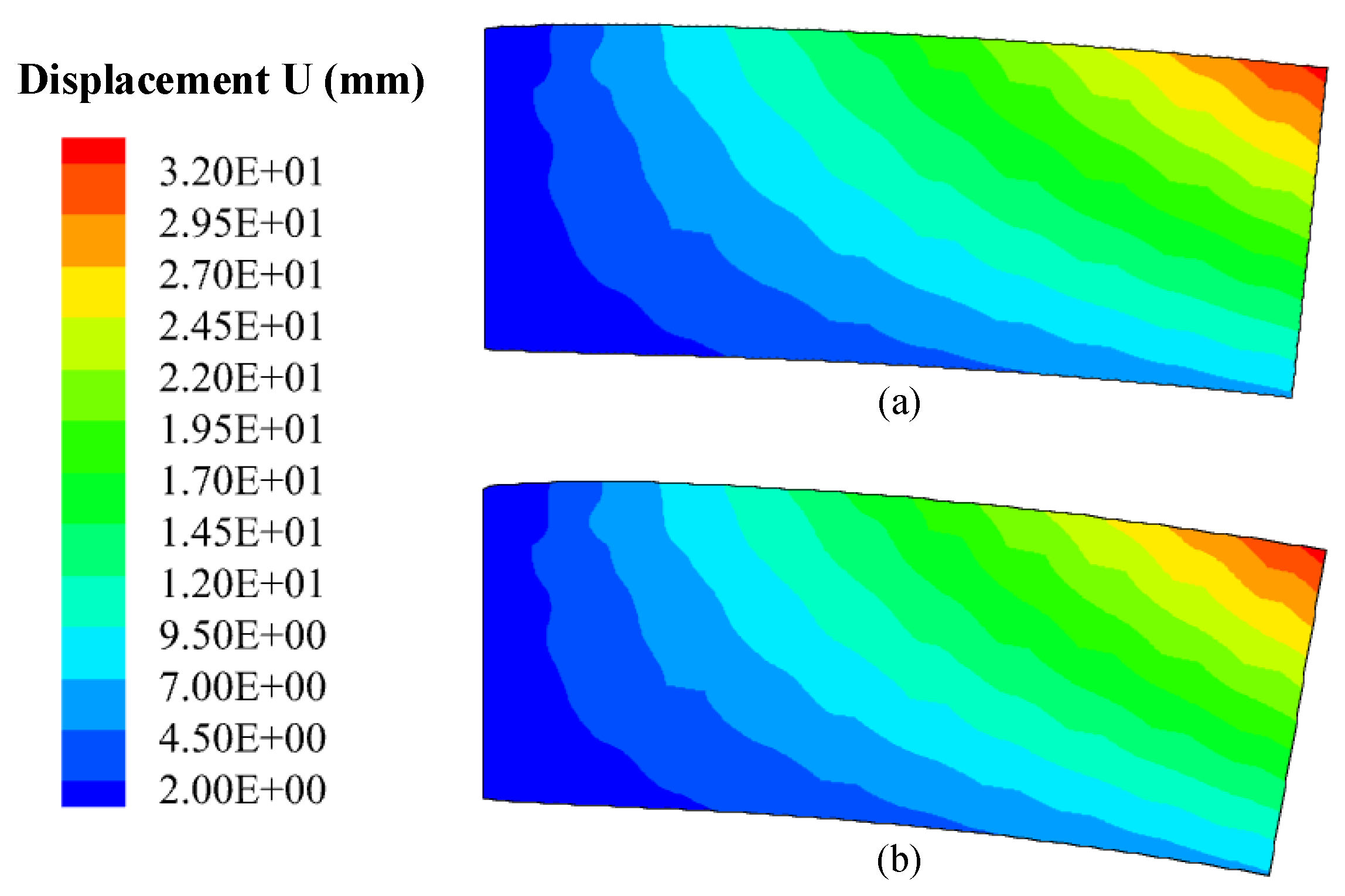
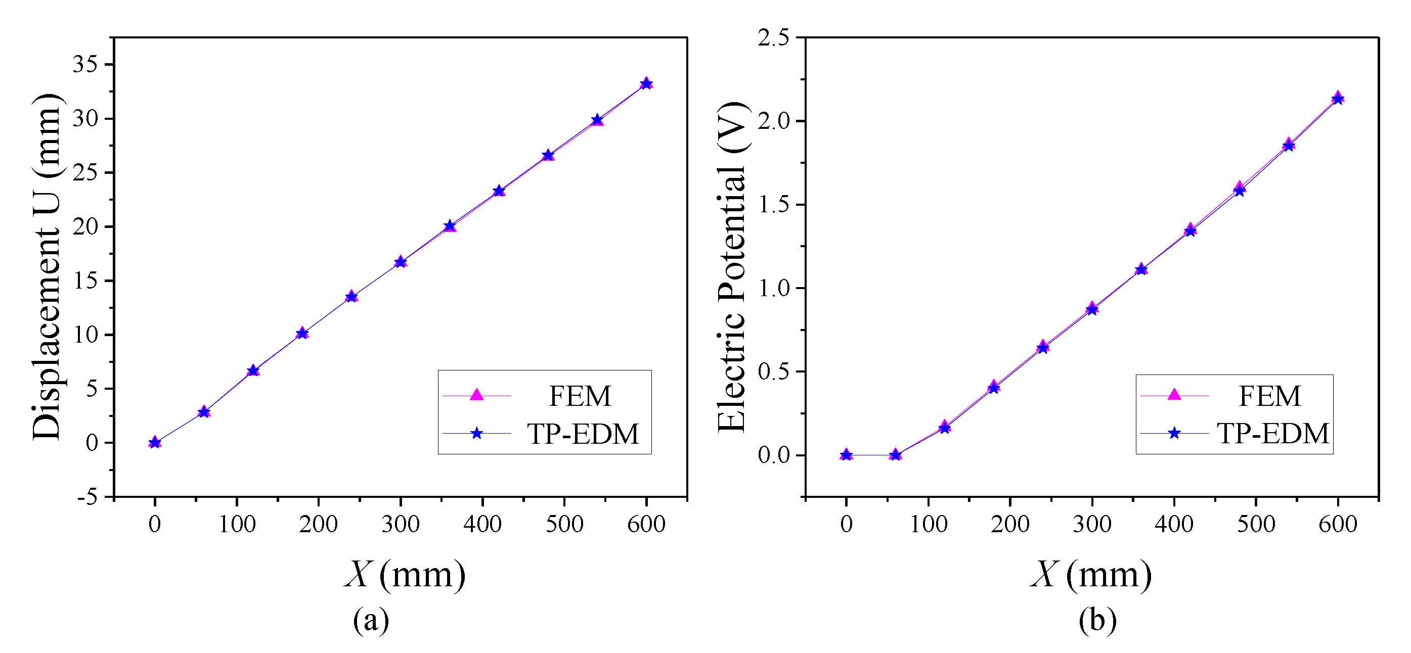
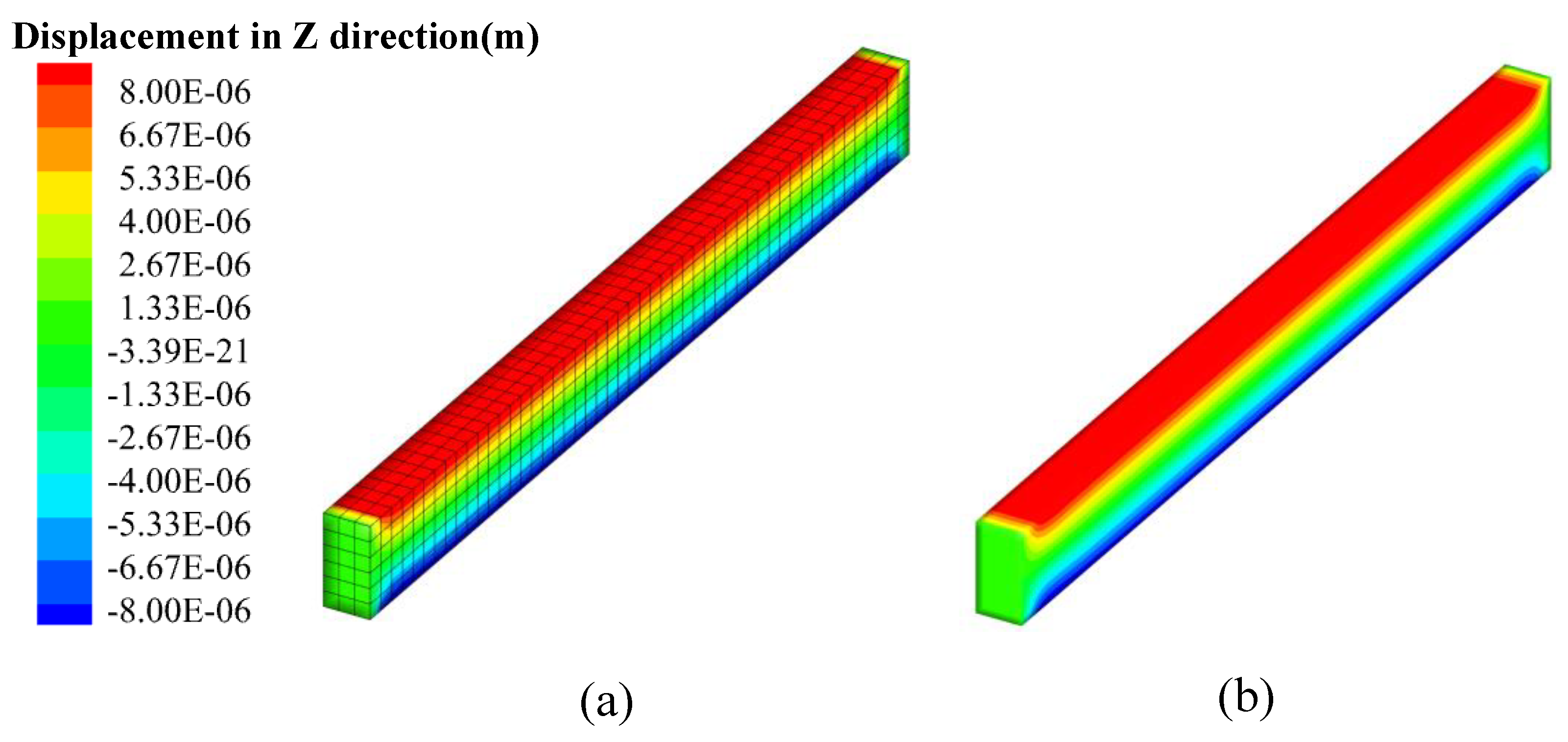
4.2. Clamped Thermal Piezoelectric 3D Beam

In this example, the thermo-electro-mechanical response of a clamped thermal piezoelectric 3D beam is considered. The two ends of the piezoelectric beam are fixed, as shown in Figure 8. The size of the beam is 0.005 m× 0.1 m × 0.01 m. Since the commercial finite element method code cannot be directly used to model the piezoelectric structures with the pyroelectric behaviors, the pyroelectric coefficients for the 3D beam are set to zero here. The other material constants can be given as follows:

$$\begin{gathered} \mathrm{E}=96.2 \mathrm{GPa},\mathsf{\mu }=0.3,\mathsf{\alpha }=8.53{\mathrm{e}}^{-6} \\ {\mathrm{e}}_{15}=-0.39{ \mathrm{cm}}^{-2},{\mathrm{e}}_{31}=-0.66{ \mathrm{cm}}^{-2},{\mathrm{e}}_{33}=1.57{ \mathrm{cm}}^{-2}, \\ {\mathsf{\lambda }}_{11}={\mathsf{\lambda }}_{22}={\mathsf{\lambda }}_{33}=8.092\times {10}^{-12}\left(\mathrm{C}•{\mathrm{V}}^{-1}{\mathrm{m}}^{-1}\right) \end{gathered}$$

Two loading cases separately composed of thermal loading and the combined thermal-electric and mechanical loading are considered in this example, respectively, to validate the effectiveness of the presented method.

Case 1: The clamped thermal piezoelectric beam structure considered is subjected to the thermal loadings. A temperature load (T = 200 K) is subjected to the beam structure, while the electrical potential is set to zero at the bottom of the structure. The piezoelectric beam will expand under the temperatures. The beam structure meshes with 900 grids. The commercial finite element codes Abaqus with the C3D8P elements are applied to validate the proposed method TP-EDM. Since the same mesh grids are utilized, the results calculated by Abaqus can be seen as the reference results.

The deformation and the electrical potential responses predicted by both TP-EDM and Abaqus can be found in Figure 9 and Figure 10, respectively. It can be found that a uniform expansion happens at most of the beam structures except the two ends, which are constrained by the fixed boundary conditions. Thus, thermal stress will be induced, which will lead to electrical potentials. At the same time, the maximum values about displacement and electrical potential induced by temperature variations in the structure can be found in

Table 2. The maximum displacement and electrical potential for the piezoelectric beam.

Methods	w (m)	φ (V)
Abaqus	1.02 × 10−5	1.76 × 105
TP-EDM	1.01 × 10−5	1.76 × 105

. Furthermore, Figure 11 gives the displacement and electrical potential for the nodes at the bottom line. The results computed by the presented method are in good agreement with those of the standard finite element method.

Case 2: In this case, the combined thermal and mechanical loadings are applied on the clamped piezoelectric beam. The upper surface of the piezoelectric beam is subjected to a uniform pressure (10MPa), while the whole model is still subjected to a temperature load of 200 K, as illustrated in Figure 8. Both of the two ends of the piezoelectric beam are fixed. At the same time, the electrical potential is set to zero at the bottom face.

In order to further verify the influence of the mesh generation type on the accuracy of the presented method, a detailed mesh refinement convergence study is performed. Three types of mesh grids are considered, consisting of 900, 5000, and 12,103 brick elements, respectively. In the last one, the irregular mesh grids with different types of hexahedral elements are considered. The deformation and the electrical potential generated by the thermal and mechanical environment can be found in Figure 12 and Figure 13, respectively. It can be found that under the combined coupled loading, the bending deformation will be generated at the clamped piezoelectric beam structure. The electrical potential generated by the mechanical loading will gather at the top surface of the structure.

Besides, it can be observed that the deformation and the electrical response predicated by TP-EDM are finely consistent with those calculated by Abaqus. The displacement and electrical potential values along the Y-axis of the upper surface of the 3D piezoelectric beam are plotted in Figure 14. At the same time, the results with different mesh grids can be found in

Table 3. Displacement in negative direction (m) and electrical potential(V) for the piezoelectric beam.

Number of Mesh Grids	w (FEM)	w (TP-EDM)	φ (FEM)	φ (TP-EDM)
900	3.44 × 10−4	3.48 × 10−4	1.75 × 10−5	1.76 × 10−5
5000	3.48 × 10−4	3.49 × 10−4	1.75 × 10−5	1.75 × 10−5
12103	3.48 × 10−4	3.49 × 10−4	1.74 × 10−5	1.75 × 10−5

. It can be seen from Figure 13 that the maximum electrical potential appeared at some part of the top surfaces, which ranges from 20 mm to 80 mm in the Y direction along the structure. Furthermore, the curve is approximately saturated in this range, shown in Figure 14b, while the maximum value happens at the center point of the structure. It can be observed that the maximum values of the displacement and electrical potential computed by the proposed method vary little with the number of the mesh grids (from 900 to 12103), which demonstrates a relatively high convergence rate of the proposed method. Thus, it can be concluded that the TP-EDM has satisfied numerical accuracy and stability to solve the coupled thermal-electrical-mechanical problems of the piezoelectric structure.

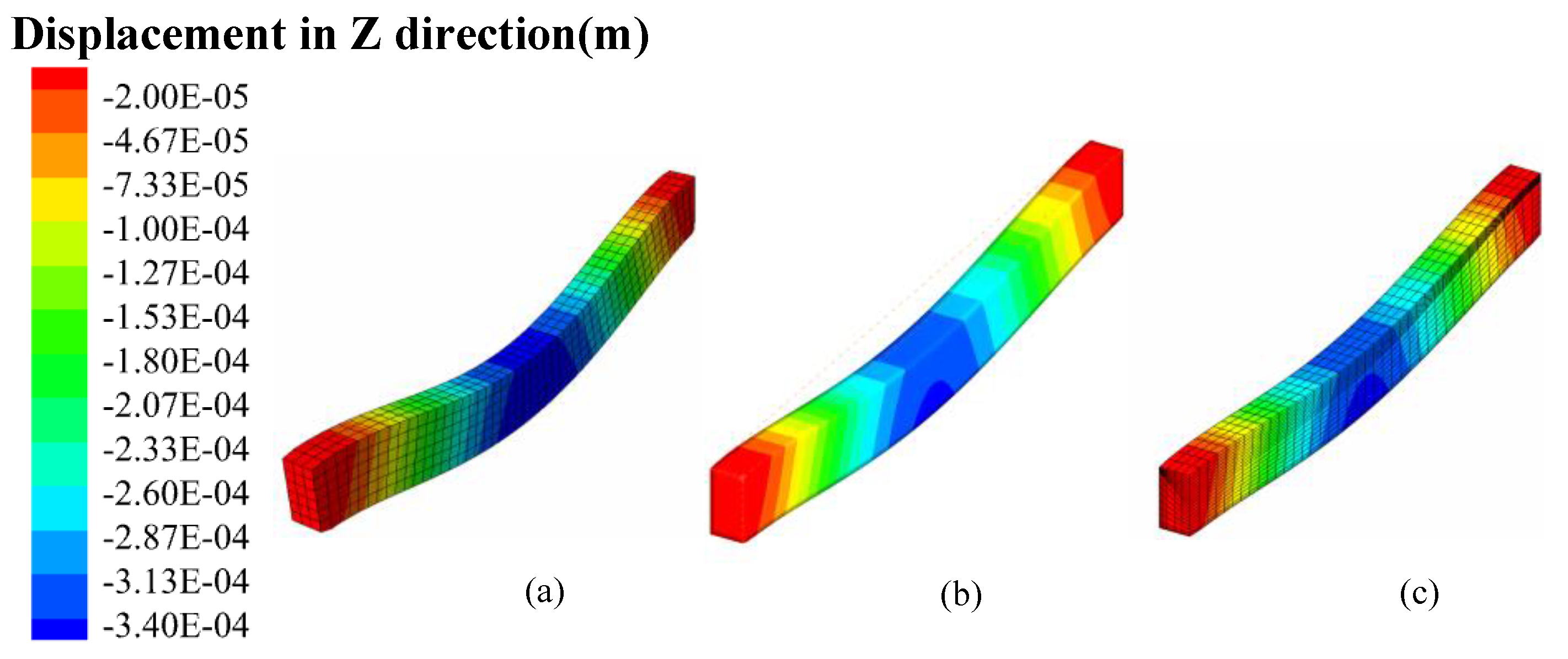
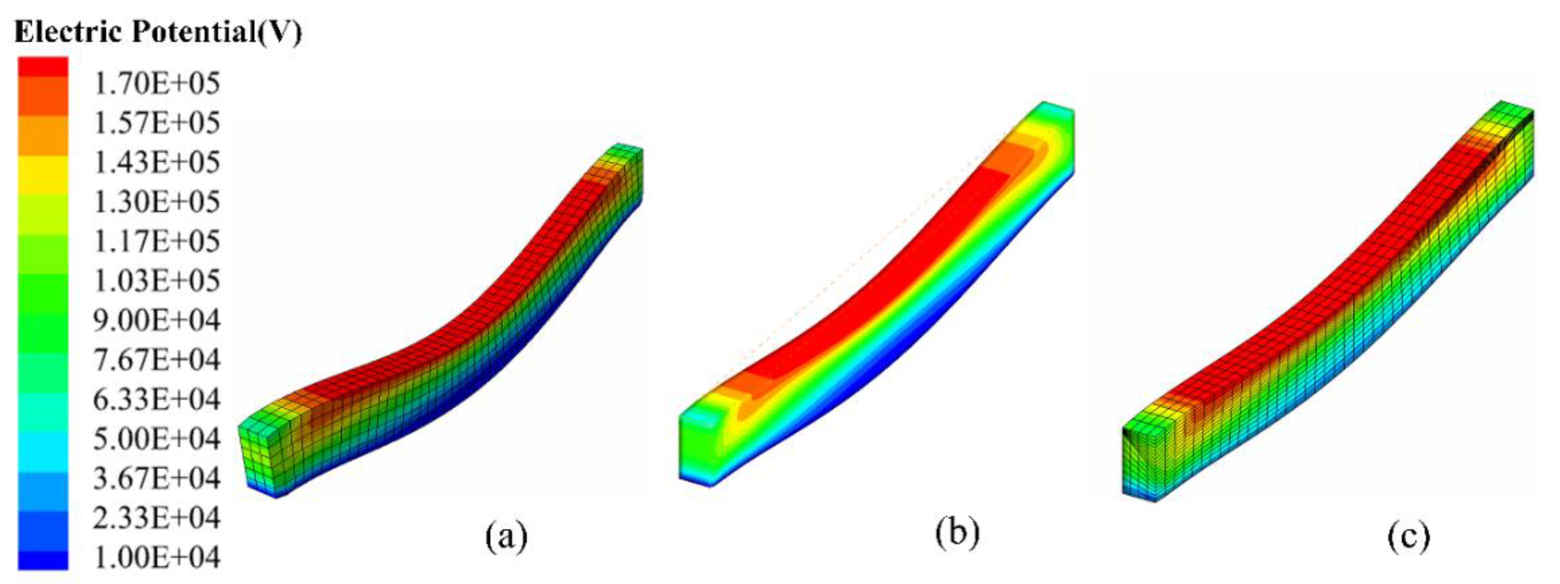
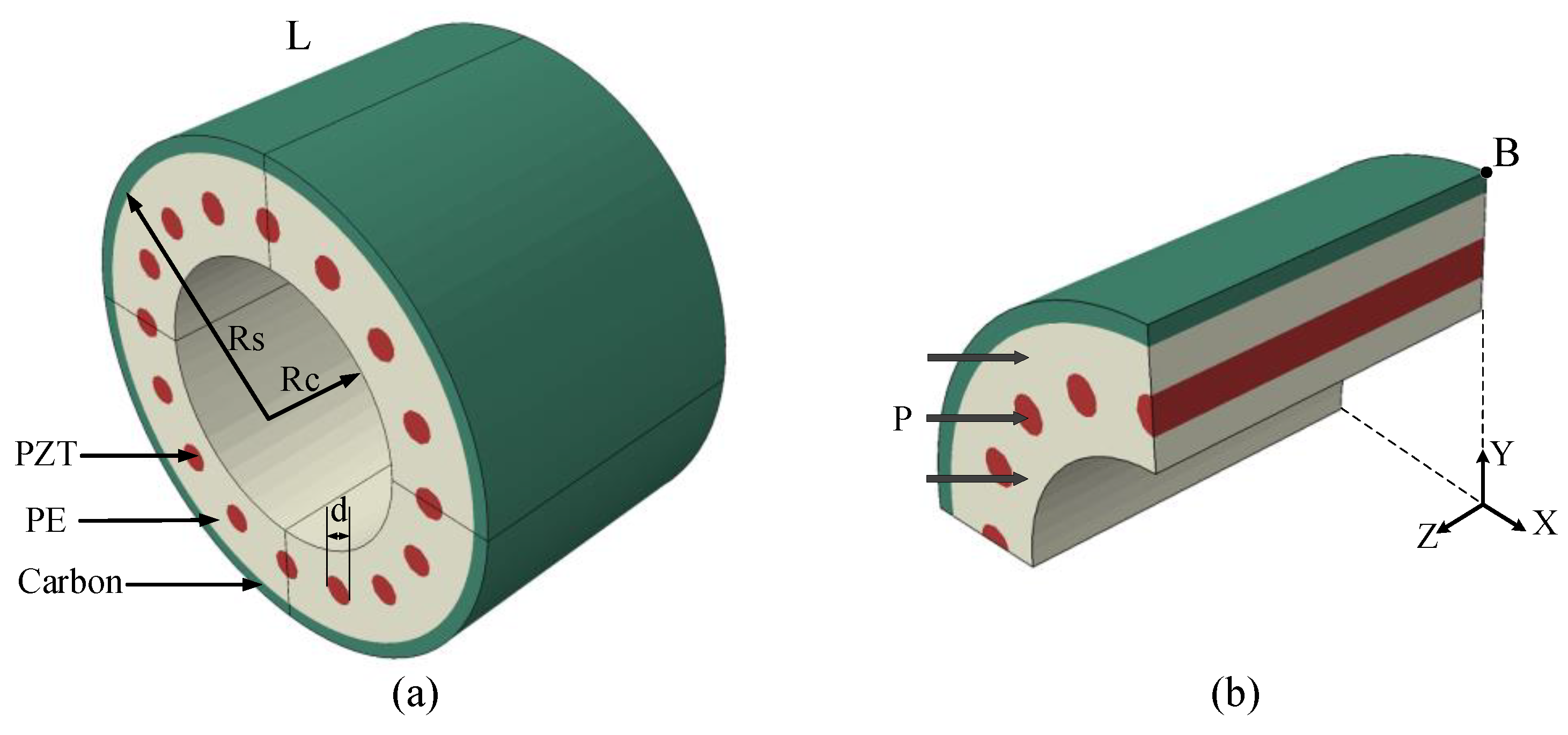
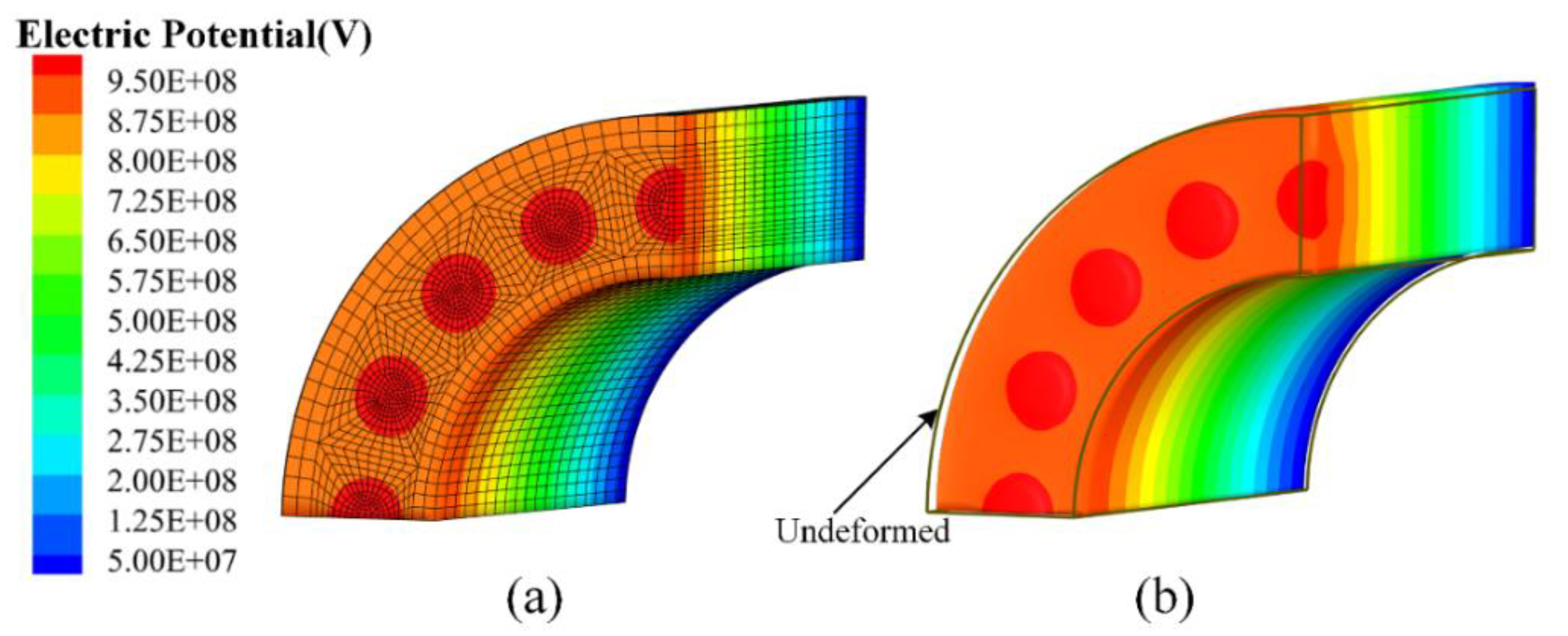
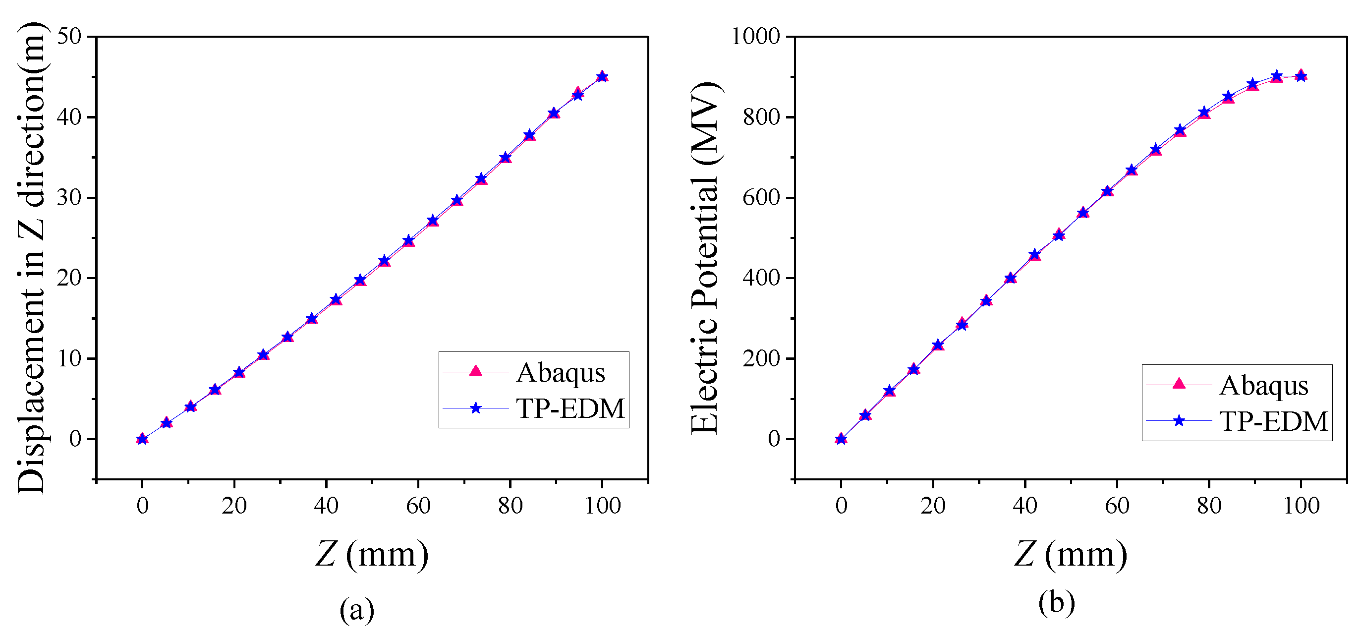
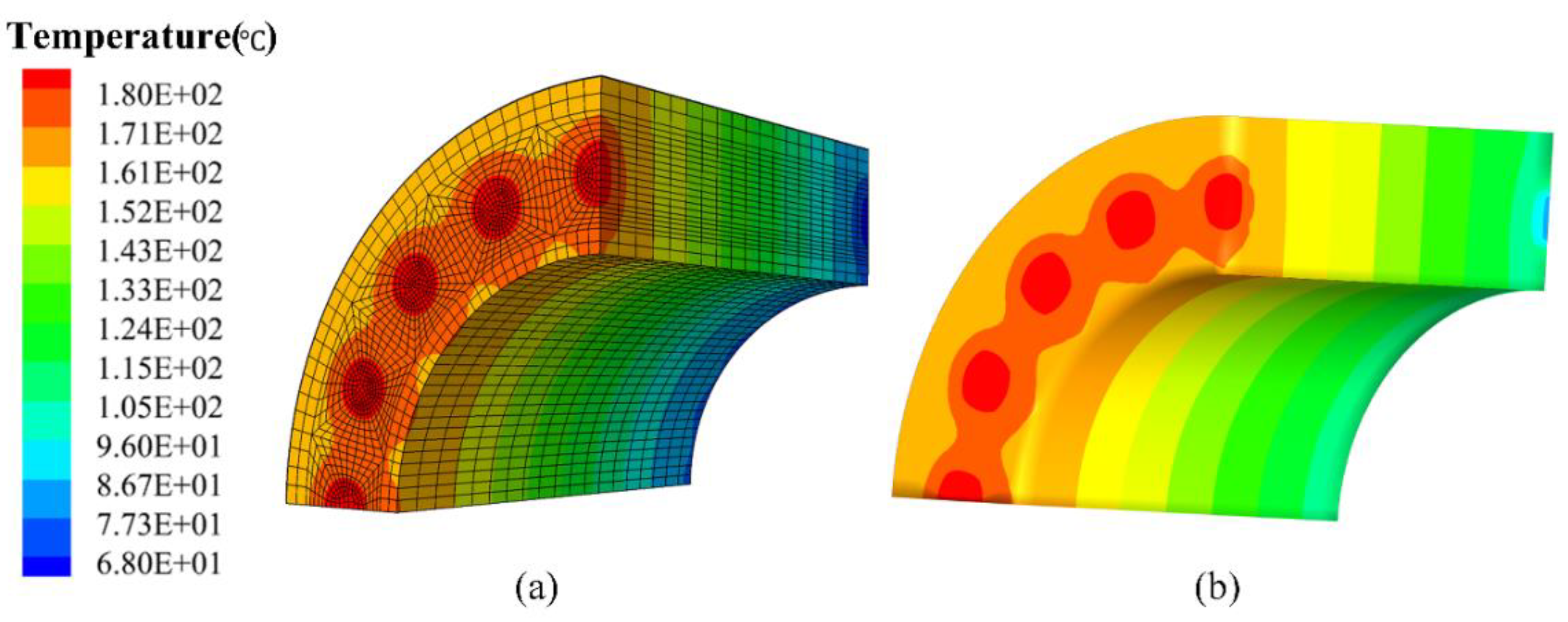
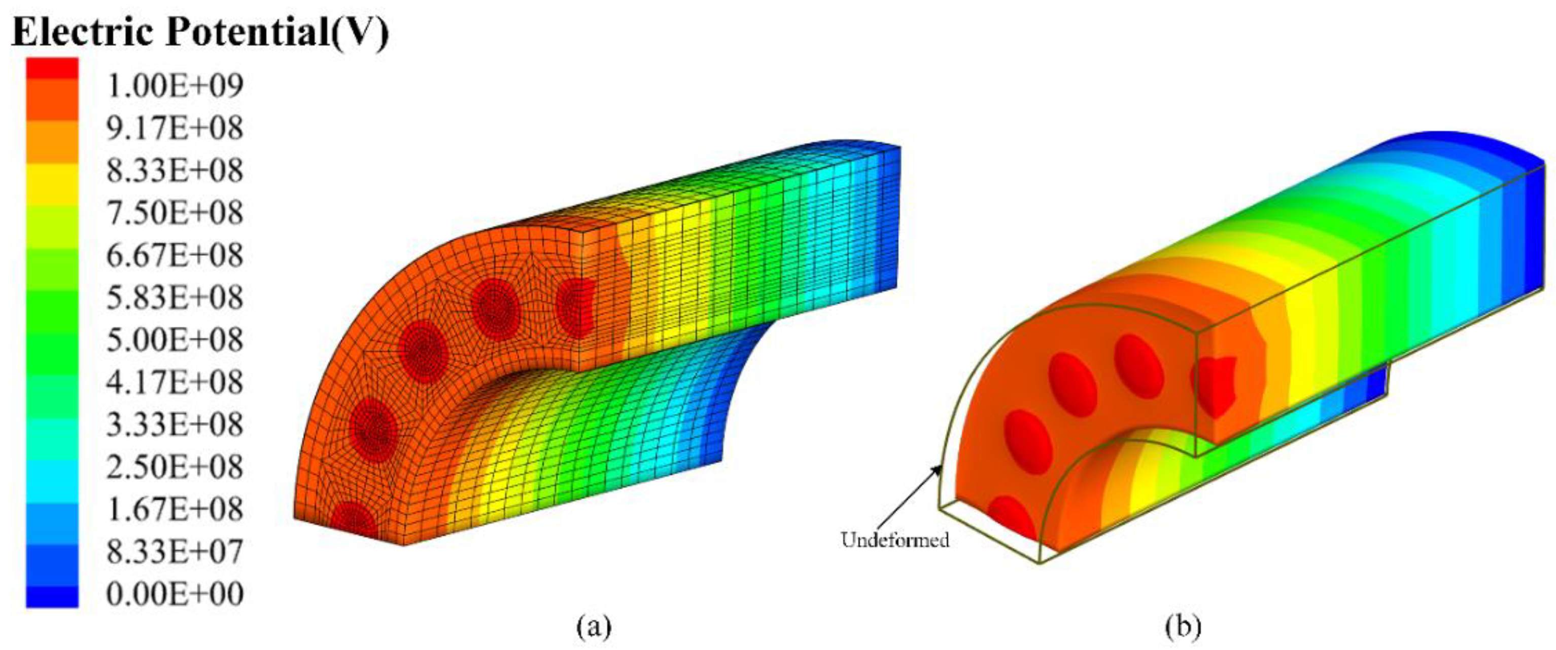
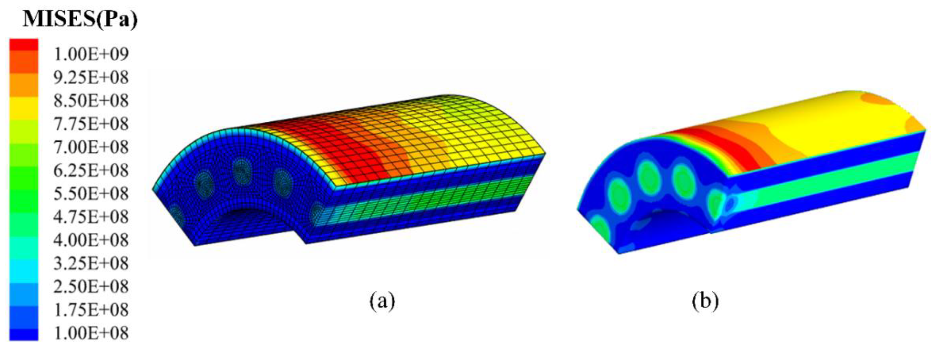
4.3. Cylindrical Structure Reinforced by Piezoelectric Fiber

In the final example, a composite structure reinforced by piezoelectric fiber under combined electro-thermo-mechanical loading is considered. This fiber-reinforced piezoelectric composite has received growing attention recently since it can provide novel properties and individual synergism between different types of materials [31]. As illustrated in Figure 15, the hollow cylindrical structure comprises a thin carbon shell, elastic core, and piezoelectric fibers. It can be found that the elastic core contains 16 sticks made of PZT. Since the model and the loading conditions are symmetric, only 1/4 model is selected to simulate the coupling behaviors. The detailed geometrical information of the structure can be found in Figure 15, in which the thickness of the carbon fiber film shell is 0.15 mm, the length of the cylinder $\mathrm{L}=100 \mathrm{mm}$, the diameter of the piezoelectric fiber $\mathrm{d}=10 \mathrm{mm}$, the radius of the hollow inclusion ${\mathrm{R}}_{\mathrm{c}}=30 \mathrm{mm}$, while the thickness of the hollow core is $\Delta ={\mathrm{R}}_{\mathrm{s}}-{\mathrm{R}}_{\mathrm{c}}=46.2 \mathrm{mm}$.

The material constants about the PZT, polyethylene (PE), and carbon of the composite structures are illustrated as follow:

PZT:
	${\mathrm{c}}_{11}=12.6,{\mathrm{c}}_{12}=5.30,{\mathrm{c}}_{13}=5.50,{\mathrm{c}}_{33}=11.7,{ \mathrm{c}}_{44}=3.53\left(\times {10}^{10 }\mathrm{N}•{\mathrm{m}}^{-2}\right)$
	${\mathrm{e}}_{15}=17,{\mathrm{e}}_{31}=-6.5,{\mathrm{e}}_{33}=23.3\left(\mathrm{C}•{\mathrm{m}}^{-2}\right)$
	${\mathsf{\lambda }}_{11}=171\times {\mathsf{\epsilon }}_0,{\mathsf{\lambda }}_{33}=147\times {\mathsf{\epsilon }}_0,{\mathsf{\epsilon }}_0=8.85419\times {10}^{-12}\left(\mathrm{C}•{\mathrm{V}}^{-1}{\mathrm{m}}^{-1}\right)$
	${\mathsf{\beta }}_{11}={\mathsf{\beta }}_{22}=1.79{\mathrm{e}}^6{\mathrm{PaK}}^{-1},{ \mathsf{\beta }}_{33}=2.03{\mathrm{e}}^6{\mathrm{PaK}}^{-1}$
	$\mathrm{k}=0.26 \mathrm{W}•{\mathrm{m}}^{-1}{\mathrm{K}}^{-1}$
PE:
	$\mathrm{E}=12.5\mathrm{GPa},\mathsf{\mu }=0.3,\mathrm{k}=0.4 2\mathrm{W}•{\mathrm{m}}^{-1}{\mathrm{K}}^{-1}$
	${\mathsf{\beta }}_{11}={\mathsf{\beta }}_{22}={\mathsf{\beta }}_{33}=2.67{\mathrm{e}}^5{\mathrm{PaK}}^{-1}$
	${\mathsf{\lambda }}_{11}={\mathsf{\lambda }}_{22}={\mathsf{\lambda }}_{33}=1.95\times {10}^{-11}\left(\mathrm{C}•{\mathrm{V}}^{-1}{\mathrm{m}}^{-1}\right)$
Carbon:
	$\mathrm{E}=180\mathrm{GPa},\mathsf{\mu }=0.34,\mathrm{k}=0.7\mathrm{W}•{\mathrm{m}}^{-1}{\mathrm{K}}^{-1}$
	${\mathsf{\beta }}_{11}={\mathsf{\beta }}_{22}={\mathsf{\beta }}_{33}=4.80{\mathrm{e}}^6{\mathrm{PaK}}^{-1}$
	${\mathsf{\lambda }}_{11}={\mathsf{\lambda }}_{22}={\mathsf{\lambda }}_{33}=8.85\times {10}^{-11}\left(\mathrm{C}•{\mathrm{V}}^{-1}{\mathrm{m}}^{-1}\right)$

In order to simulate the coupled response of the piezoelectric fiber-reinforced composites, two loading cases are considered. In the first case, the loading and boundary conditions could be described as below: at the bottom of the structure (Z = 0), the electrical potential is set to zero, the normal displacement is constrained, the temperature is set to 20 °C. At the same time, the applied pressure is 100 MPa at the top face of the structure (Z = 100), while the temperature of the face is 100 °C. The boundary condition can be listed as follow:

$$\begin{gathered} \mathrm{Z}=0:\mathsf{\varphi }=0; \mathrm{U}=0; \mathrm{T}=20 ℃ \\ \mathrm{Z}=100: \mathrm{P}=100 \mathrm{MPa}; \mathrm{T}=100 ℃ \end{gathered}$$

The piezoelectric fiber-reinforced composite cylindrical structure meshes with 23,902 elements. The displacement and electrical potential result of the 1/4 structure calculated by TP-EDM and Abaqus are given in Figure 16 and Figure 17. The displacement and electrical potential data along the line at the position ($\mathrm{X}=0,\mathrm{Y}=76.35 \mathrm{mm})$ are given in Figure 18. It can be seen from Figure 18 that the displacement and potential results curves calculated by TP-EDM are basically consistent as those calculated by Abaqus in the coupling problem of heat conduction and mechanical force. Moreover, the displacement and electrical potential created by Abaqus and TP-EDM of the one point (point B) on the structure are listed in

Table 4. The displacement and electrical potential for Point B at the piezoelectric cylinder.

Method	w (m)	φ (V)
Abaqus	4.49 × 10−2	9.03 × 108
TP-EDM	4.47 × 10−2	9.02 × 108

. It was evident that the results obtained by these two methods are well-matched, although different types of materials are considered.

For the second case, to verify the accuracy and diversity of the method, the combined thermo-electro-mechanical boundary condition is considered in this example. The heat exchange boundary conditions are applied on the two end faces of the piezoelectric fibers. As indicated in Figure 15a, at one end of the cylinder, the heat flux of the PZT face is set to $q=0.2{ \mathrm{Wm}}^{-2} ℃$, while the reference temperature is 60 °C. At the other end, the heat flux is set to $q=0.1{ \mathrm{Wm}}^{-2} ℃$, while the environmental temperature is 200 °C. These boundary conditions applied on the target structure are listed as follow:

PZT fibers:

$$\begin{gathered} \mathrm{Z}=0: \mathrm{T}=60 ℃ \mathrm{q}=0.2{ \mathrm{Wm}}^{-2} ℃ ; \\ \mathrm{Z}=-100: \mathrm{T}=200 ℃ \mathrm{P}=100 \mathrm{MPa} \mathrm{q}=0.1{ \mathrm{Wm}}^{-2} ℃ . \end{gathered}$$

The mesh grid used in this case is the same as that for the first case. The temperature distribution of the cylindrical structure calculated by Abaqus and TP-EDM is shown in Figure 19. It can be observed that as the heat flux is only applied on the end of the piezoelectric fibers, the resulting temperature at corresponding areas is higher than that of the matrix. The temperature calculated by TP-EDM agrees well with that simulated by ABAQUS, which shows the accuracy of TP-EDM in solving the heat transfer problem.

Furthermore, once the calculated temperature is calculated for the piezoelectric composite structure, the other high order responses such as the electrical potential and stress can be further calculated by the proposed method. As illustrated in Figure 20 and Figure 21, the left end with higher temperatures generates high electric potentials. At the same time, the von Mises stress results mainly happen at the shell surrounding the cylinder caused by the thermal expansion of the core. Moreover, the computed results by TP-EDM are in good agreement with those calculated by Abaqus. Therefore, we can conclude that TP-EDM can obtain the results with satisfying accuracy in dealing with the piezoelectric composites subjected to combined thermo-electrical-mechanical loadings. Further, since thermal loads are directly utilized in the governing equations to establish the system of equations without any domain integrations, the proposed method can reduce the complexity in dealing with the thermal coupling problems of the piezoelectric structures.

5. Conclusions

In this study, a new strong form method, the elemental differential method, has been proposed to simulate the coupled response of the piezoelectric structures subjected to combined thermal-electric-mechanical loadings. The main contribution of this method is to derive the analytical formulas for combining the governing equations of the piezoelectric problem and the heat conduction problem directly. Based on the proposed method, the thermal conduction and thermal, mechanical problems for the thermal-electric-mechanical problem can be resolved with the same strategy. Meanwhile, the pyroelectric effect considering the relationship between thermal and electrical fields is directly addressed.

Several numerical examples, including the piezoelectric composites, are utilized to evaluate the effectiveness of the proposed method. From the comparison of the results calculated by different methods based on the standard finite element framework, it can be found that the proposed method can extract the benefits from the point collocation methods (PCM) and standard finite element methods. Furthermore, the proposed method’s final equations about elastic and electric field variables could be constructed from the isoparametric mesh grid without any domain integration. It also can be found that the system of equations for the heat transfer and thermal-elastic response of the piezoelectric problems can be generated in a unified way. At the same time, the effect of thermal expansion can be directly handled. Furthermore, in the proposed method, the pyroelectric effects of the piezoelectric structure can be directly substituted into the system of equations through the collocation technique without any domain integrations. This provides a convenient technique for future research on the pyroelectric effects in actual engineering applications.

References

1. Yu, X.; Wang, H.; Ning, X. Needle-shaped ultrathin piezoelectric microsystem for guided tissue targeting via mechanical sensing. Nat. Biomed. Eng. 2018, 2, 165–172. [Google Scholar] [CrossRef]
2. Liu, Y.; Zhao, L.; Wang, L. Skin-Integrated graphene-embedded lead Zirconate Titanate rubber for energy harvesting and mechanical sensing. Adv. Mater. Technol. 2019, 4, 1900744. [Google Scholar] [CrossRef]
3. Tariq, M.H.; Younas, U.; Dang, H.; Ren, J. A general solution for three dimensional steady-state transversely isotropic hygro-thermo-magneto-piezoelectric media. Appl. Math. Model. 2020, 80, 625–646. [Google Scholar] [CrossRef]
4. Gülay, A.M.; Cengiz, D. Certain hygrothermopiezoelectric multi-field variational principles for smart elastic laminae. Mech. Adv. Mater. Struct. 2008, 15, 21–32. [Google Scholar] [CrossRef]
5. Wang, X.Q.; Fu, T.C.; Chan, K.H. In-built thermo-mechanical cooperative feedback mechanism for self-propelled multimodal locomotion and electricity generation. Nat. Commun. 2018, 9, 3438. [Google Scholar] [CrossRef]
6. Wang, X.Q.; Chan, K.H.; Cheng, Y. Somatosensory, Light-Driven, Thin-Film Robots Capable of Integrated Perception and Motility. Adv. Mater. 2020, 32, 2000351. [Google Scholar] [CrossRef]
7. Song, K.; Zhao, R.; Wang, Z.L. Conjuncted Pyro-Piezoelectric Effect for Self-Powered Simultaneous Temperature and Pressure Sensing. Adv. Mater. 2019, 31, 1902831.1–1902831.9. [Google Scholar] [CrossRef] [PubMed]
8. Fantoni, F.; Bacigalupo, A.; Paggi, M. Design of thermo-piezoelectric microstructured bending actuators via multi-field asymptotic homogenization. Int. J. Mech. Sci. 2018, 146–147, 319–336. [Google Scholar] [CrossRef] [Green Version]
9. Batra, A.; Aggarwal, M. Pyroelectric Materials: Infrared Detectors, Particle Accelerators and Energy Harvesters; SPIE Press: Bellingham, WA, USA, 2013; Chapter 1; ISBN 9780819493316. [Google Scholar]
10. Nan, C.; Bichurin, M.; Dong, S.; Viehland, D.; Srinivasan, G. Multiferroic magnetoelectric composites: Historical perspective, status, and future directions. J. Appl. Phys. 2008, 103, 031101. [Google Scholar] [CrossRef]
11. Tan, P.; Tong, L. Modeling for the electro-magneto-thermo-elastic properties of piezoelectric-magnetic fiber reinforced composites. Compos. Part A Appl. Sci. Manuf. 2002, 33, 631–645. [Google Scholar] [CrossRef]
12. Ashida, F.; Sakata, S.I.; Matsumoto, K. Structure design of a poiezoelectric composite disk for control of thermal stress. J. Appl. Mech. 2008, 75, 061009. [Google Scholar] [CrossRef]
13. Taya, N.M.; Namli, O.C. Design of piezo-SMA composite for thermal energy harvester under fluctuating temperature. J. Appl. Mech. 2011, 78, 2388–2399. [Google Scholar] [CrossRef]
14. Srivastava, V.; Song, Y.; Bhatti, K.; James, R.D. The direct conversion of heat to electricity using multiferroic alloys. Adv. Energy Mater. 2011, 1, 97–104. [Google Scholar] [CrossRef]
15. Ang, S.; Brachelet, F.; Breaban, F.; Defer, D. Defect detection in CFRP by infrared thermography with CO2 Laser excitation compared to conventional lock-in infrared thermography. Compos. Part B 2015, 69, 1–5. [Google Scholar] [CrossRef]
16. Sladek, J.; Sladek, V.; Wunsche, M.; Tan, C.-L. Crack analysis of size-dependent piezoelectric solids under a thermal load. Eng. Fract. Mech. 2017, 182, 187–220. [Google Scholar] [CrossRef]
17. Rahman, A.A.A. Influence of the Perforation Configuration on the Dynamic Behavior of Multilayered Beam Structure. Structures 2020, 28, 1413–1426. [Google Scholar] [CrossRef]
18. Jiang, J.P.; Li, D.X. A new finite element model for piezothermoelastic composite beam. J. Sound Vib. 2007, 306, 849–864. [Google Scholar] [CrossRef]
19. Amini, Y.; Emdad, H.; Farid, M. Finite element modeling of functionally graded piezoelectric harvesters. Compos. Struct. 2015, 129, 165–176. [Google Scholar] [CrossRef]
20. Yan, Z.; Jiang, L. On a moving dielectric crack in a piezoelectric interface with spatially varying properties. Eng. Fract. Mech. 2009, 76, 560–579. [Google Scholar] [CrossRef]
21. Shi, J.; Akbarzadeh, A.H. Architected cellular piezoelectric metamaterials: Thermo-electro-mechanical properties. Acta Mater. 2019, 163, 91–121. [Google Scholar] [CrossRef]
22. Lv, J.; Yang, K.; Zhang, H.; Yang, D.; Huang, Y. A hierarchical multiscale approach for predicting thermo-electro-mechanical behavior of heterogeneous piezoelectric smart materials. Comput. Mater. Sci. 2014, 87, 88–99. [Google Scholar] [CrossRef]
23. Wang, D.D.; Wang, J.R.; Wu, J.C. Superconvergent gradient smoothing meshfree collocation method. Comput. Methods Appl. Mech. Eng. 2018, 340, 728–766. [Google Scholar] [CrossRef]
24. Gu, Y.T.; Liu, G.R. A meshfree weak-strong (MWS) form method for time dependent problems. Comput. Mech. 2005, 35, 134–145. [Google Scholar] [CrossRef]
25. Gao, X.W.; Li, Z.Y.; Yang, K. Element differential method and its application in thermal-mechanical problems. Int. J. Numer. Methods Eng. 2018, 113, 82–108. [Google Scholar] [CrossRef]
26. Moradi-Dastjerdi, R.; Radhi, A.; Behdinan, K. Damped dynamic behavior of an advanced piezoelectric sandwich plate. Compos. Struct. 2020, 243, 12243. [Google Scholar] [CrossRef]
27. Liew, K.M.; Yang, J.; Kitipornchai, S. Postbuckling of piezoelectric FGM plates subject to thermo-electro-mechanical loading. Int. J. Solids Struct. 2003, 40, 3869–3892. [Google Scholar] [CrossRef]
28. Alashti, R.A.; Khorsand, M. Three-dimensional thermo-elastic analysis of a functionally graded cylindrical shell with piezoelectric layers by differential quadrature method. Int. J. Press. Vessel. Pip. 2011, 88, 167–180. [Google Scholar] [CrossRef]
29. Lv, J.; Shao, M.J.; Cui, M.; Gao, X.W. An efficient collocation approach for piezoelectric problems based on the element differential method. Compos. Struct. 2019, 230, 111483. [Google Scholar] [CrossRef]
30. Gao, X.W.; Huang, S.Z.; Cui, M. Element differential method for solving general heat conduction problems. Int. J. Heat Mass Transfer. 2017, 115, 882–894. [Google Scholar] [CrossRef]
31. Mosallaie, B.A.A.; Ghorbanpour, A.A.; Kolahchi, R.; Mozdianfard, M.R. Electro-thermo-mechanical torsional buckling of a piezoelectric polymeric cylindrical shell reinforced by DWBNNTs with an elastic core. Appl. Math. Model. 2012, 36, 2983–2995. [Google Scholar] [CrossRef] [Green Version]
Figure 1. The piezoelectric structure subjected to combined thermo-electro-mechanical loadings.
Coatings 11 00687 g001
Figure 2. The Lagrange isoparametric elements: (a) spatial coordinates x (b) intrinsic coordinates ξ .
Coatings 11 00687 g002
Figure 3. The internal nodes, interface nodes and outer surface nodes in the computational domain.
Coatings 11 00687 g003
Figure 4. The cantilever piezoelectric beam structure composed of 4 × 10-unit cells.
Coatings 11 00687 g004
Figure 5. Displacement in the X direction (U) of the cantilever beam calculated by (a) FEM (b) TP-EDM.
Coatings 11 00687 g005
Figure 6. Electric potential of the cantilever beam calculated by (a) FEM and (b) TP-EDM.
Coatings 11 00687 g006
Figure 7. (a) Displacement in the X direction (U) and (b) Electrical potential along Y = 240 mm of piezoelectric structure.
Coatings 11 00687 g007
Figure 8. The 3D piezoelectric beam subjected to the combined thermal-elastic-mechanical loadings.
Coatings 11 00687 g008
Figure 9. Displacement in the Z direction obtained by (a) Abaqus and (b) TP-EDM.
Coatings 11 00687 g009
Figure 10. Electrical potential of the clamped piezoelectric 3D beam calculated by (a) Abaqus and (b) TP-EDM.
Coatings 11 00687 g010
Figure 11. (a) Displacement in the Z direction and (b) electrical potential along the Y-axis of the piezoelectric structure.
Coatings 11 00687 g011
Figure 12. Displacement in Z direction calculated by (a) FEM based on regular mesh (b) TP-EDM based on regular mesh, (c) TP-EDM based on the irregular mesh.
Coatings 11 00687 g012
Figure 13. Electrical potential calculated by (a) FEM based on regular mesh, (b) TP-EDM based on regular mesh, (c) TP-EDM based on irregular mesh grids.
Coatings 11 00687 g013
Figure 14. (a) Displacement in the Z direction and (b) electrical potential along the Y-axis of the piezoelectric structure.
Coatings 11 00687 g014
Figure 15. (a) The piezoelectric fiber-reinforced composite cylindrical structure and (b) 1/4 geometry for the simulation.
Coatings 11 00687 g015
Figure 16. The displacement in the Z direction of the piezoelectric composites computed by (a) Abaqus and (b) TP-EDM.
Coatings 11 00687 g016
Figure 17. The electrical potential of the piezoelectric composites calculated by (a) Abaqus and (b) TP-EDM.
Coatings 11 00687 g017
Figure 18. (a) Displacement in the Z-direction and (b) electrical potential along X = 0 , Y = 76.35   mm of the piezoelectric structure.
Coatings 11 00687 g018
Figure 19. The temperature distribution on the piezoelectric cylinder calculated from (a) Abaqus and (b) TP-EDM.
Coatings 11 00687 g019
Figure 20. Electrical Potential of the piezoelectrical cylinder calculated by (a) Abaqus and (b) TP-EDM.
Coatings 11 00687 g020
Figure 21. Von Mises pressure of the piezoelectrical cylinder calculated by (a) Abaqus and (b) TP-EDM.
Coatings 11 00687 g021