On Soliton Solutions of Perturbed Boussinesq and KdV-Caudery-Dodd-Gibbon Equations

Abstract

Nonlinear science is a fundamental science frontier that includes research in the common properties of nonlinear phenomena. This article is devoted for the study of new extended hyperbolic function method (EHFM) to attain the exact soliton solutions of the perturbed Boussinesq equation (PBE) and KdV–Caudery–Dodd–Gibbon (KdV-CDG) equation. We can claim that these solutions are new and are not previously presented in the literature. In addition, 2d and 3d graphics are drawn to exhibit the physical behavior of obtained new exact solutions.

1. Introduction

The analysis of exact solutions to nonlinear evolution equations (NLEEs) is fundimental to the study of nonlinear properties. NLEEs are extensively used to illustrate complex materialistic development in numerous zones of sciences, chiefly in fluid mechanics, chemical diffusion dynamics, ion acoustics, atmospheric physics, solid-state mechanics, and nonlinear vibrations [1,2,3,4,5,6,7,8].

Researchers put much effort into obtaining the exact systematic solutions to nonlinear partial differential equations (NLPDEs). Efficient techniques for extracting exact solutions to NLEEs have been reported by many researchers, such as the Jacobi elliptic function expansion method [9,10,11], tanh method [12,13,14], exp-function method [15,16], F-expansion methods [17,18,19,20,21], ansatz function method [22], auxiliary differential equation method [23,24], homogeneous balance method [25,26], $(G^{\prime }/G)$-expansion method [27,28], modified simple equation method [29], trail function method [30,31], the variational method [32,33,34], sub-ODE method [35], function transformation method [36,37,38], new EHFM [39,40,41,42], and many more.

In this article, a modern technique, namely new EHFM [39,40,41], is utilized to retrieve solutions to PBE and KdV-CDG equations arising in acoustic waves, long water waves, quantum mechanics, plasma waves, and nonlinear optics. The main advantage of using method EHFM is to construct the dark, bright, singular, and periodic soliton solutions.

2. The Extended Hyperbolic Function Method

Consider nonlinear PDEs as follows:

$$\begin{array}{c}\hfill G(\upsilon ,{\upsilon }_t,{\upsilon }_x,{\upsilon }_{xt},{\upsilon }_{xx},\dots )=0,\end{array}$$

(1)

where G is a nonlinear function. Let $\upsilon (x,t)=\upsilon \left(\theta \right)$, $\theta =kx+\eta t$ which transforms (1) into the following ODE:

$$\begin{array}{c}\hfill H(\upsilon ,{\upsilon }^{\prime },{\upsilon }^{″},\dots )=0.\end{array}$$

(2)

The steps of the EHFM [37,38,39,40,41] are presented by following two forms:

Form 1: Let the solution of (2) be given as

$$\begin{array}{c}\hfill u\left(\xi \right)=\sum _{i=0}^N{a}_i{T}^i\left(\xi \right),a_{\mathbb{N}}\ne 0,\end{array}$$

(3)

where $a_i(0\le i\le N)$ are coefficients and $T\left(\xi \right)$ satisfies the following ODE

$$\begin{array}{c}\hfill T^{\prime }\left(\xi \right)=\frac{dT}{d\xi }=T\sqrt{c+d{T}^2},c,d\in R.\end{array}$$

(4)

N can be calculated by applying balancing principle on ODE. Using (2)–(4) and by taking coefficients of powers of T equal to zero, a set of algebraic equations is obtained. After solving obtained set of equations, one can derive all values of the involved coefficients. The general solutions to ODE (4) have the following types

Set 1: When $c>0$, $d>0$,

$$\begin{array}{c}\hfill T_1\left(\xi \right)=-\sqrt{\frac{c}{d}}csch\sqrt{c}(\xi +{\xi }_0),\end{array}$$

(5)

Set 2: When $c<0$, $d>0$,

$$\begin{array}{c}\hfill T_2\left(\xi \right)=\sqrt{\frac{-c}{d}}sec\sqrt{-c}(\xi +{\xi }_0),\end{array}$$

(6)

Set 3: When $c>0$, $d<0$,

$$\begin{array}{c}\hfill T_3\left(\xi \right)=\sqrt{\frac{c}{-d}}sech\sqrt{c}(\xi +{\xi }_0),\end{array}$$

(7)

Set 4: When $c<0$, $d>0$,

$$\begin{array}{c}\hfill T_4\left(\xi \right)=\sqrt{\frac{-c}{d}}csc\sqrt{-c}(\xi +{\xi }_0),\end{array}$$

(8)

Set 5: When $c>0$, $d=0$,

$$\begin{array}{c}\hfill T_5\left(\xi \right)=exp\left[\sqrt{c}(\xi +{\xi }_0)\right],\end{array}$$

(9)

Set 6: When $c<0$, $d=0$,

$$\begin{array}{c}\hfill T_6\left(\xi \right)=cos\sqrt{-c}(\xi +{\xi }_0)+\iota sin\sqrt{-c}(\xi +{\xi }_0),\end{array}$$

(10)

Set 7: When $c=0$, $d>0$,

$$\begin{array}{c}\hfill T_7\left(\xi \right)=\pm \frac{1}{\sqrt{d}(\xi +{\xi }_0)},\end{array}$$

(11)

Set 8: When $c=0$, $d<0$,

$$\begin{array}{c}\hfill T_8\left(\xi \right)=\pm \frac{\iota }{\sqrt{-d}(\xi +{\xi }_0)}.\end{array}$$

(12)

Form 2: Let the ODE in (2) have exact solution of the form (3) and let $T\left(\xi \right)$ satisfy ODE

$$\begin{array}{c}\hfill T^{\prime }\left(\xi \right)=\frac{dT}{d\xi }=c+d{T}^2,c,d\in R,\end{array}$$

(13)

Substituting (3) into (2) and applying (14), we attain a set of algebraic equations. We get all values of the involved constants by solving the obtained set of equations. The ODE (13) has the following types of solutions

Set 1: When $cd>0$,

$$\begin{array}{c}\hfill T_1\left(\xi \right)=sgn\left(c\right)\sqrt{\frac{c}{d}}tan\left(\sqrt{cd}(\xi +{\xi }_0)\right),\end{array}$$

(14)

Set 2: When $cd>0$,

$$\begin{array}{c}\hfill T_2\left(\xi \right)=-sgn\left(c\right)\sqrt{\frac{c}{d}}cot\left(\sqrt{cd}(\xi +{\xi }_0)\right),\end{array}$$

(15)

Set 3: When $cd<0$,

$$\begin{array}{c}\hfill T_3\left(\xi \right)=sgn\left(c\right)\sqrt{-\frac{c}{d}}tanh\left(\sqrt{-cd}(\xi +{\xi }_0)\right),\end{array}$$

(16)

Set 4: When $cd<0$,

$$\begin{array}{c}\hfill T_4\left(\xi \right)=sgn\left(c\right)\sqrt{-\frac{c}{d}}coth\left(\sqrt{-cd}(\xi +{\xi }_0)\right),\end{array}$$

(17)

Set 5: When $c=0$, $d>0$,

$$\begin{array}{c}\hfill T_5\left(\xi \right)=-\frac{1}{d(\xi +{\xi }_0)},\end{array}$$

(18)

Set 6: When $c<0$, $d=0$,

$$\begin{array}{c}\hfill T_6\left(\xi \right)=c(\xi +{\xi }_0).\end{array}$$

(19)

The multiple exact special solutions of nonlinear PDE (1) are acquired using (3) and (14)–(19).

Notice that the sign is the familiar sign function.

Remarks: The constraints of Equations (5)–(12) and (14)–(19) are uniformly suitable. From sets 1–4 of Equations (14)–(17), their conditions are influenced by the evidence that (13) has the form of the following Riccati equation.

(i) $\frac{dT}{d\xi }=c(1-T^2),$ which has solution of the form [42].

(ii) $T\left(\xi \right)=\frac{c-dexp(-2c\xi )}{c+dexp(-2c\xi )},$ where c and d are arbitrary constants which satisfy $c^2+d^2\ne 0$. Depending on the results in [43], one can attain the miscellaneous forms of Equations (14)–(17) and their conditions from the analysis of the inconsistent constants of (ii).

Step 4. After obtaining the value of N, we will compare coefficients of all the powers of $T\left(\xi \right)$ and obtain a system of algebraic equations from the resultant equations.

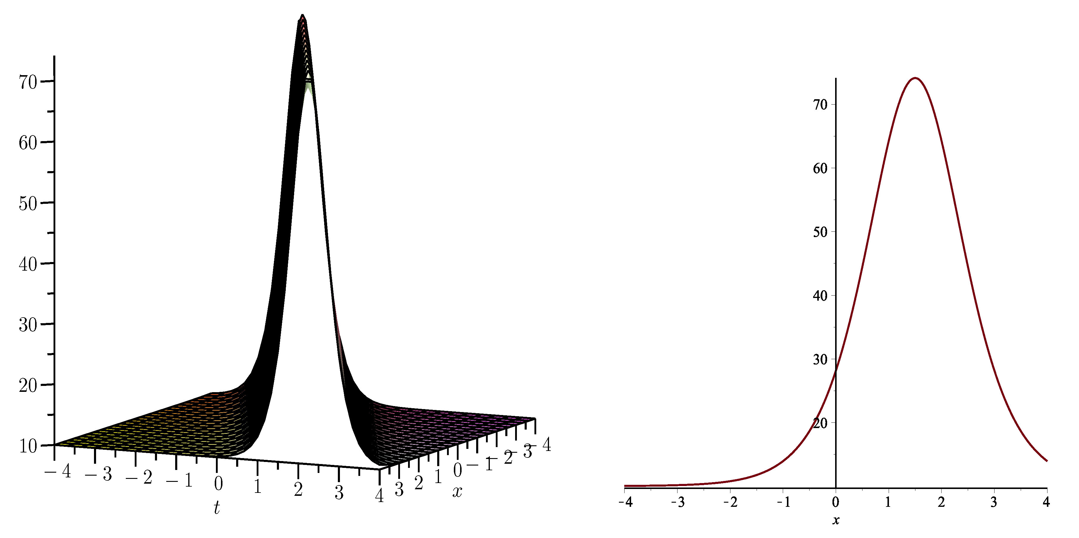
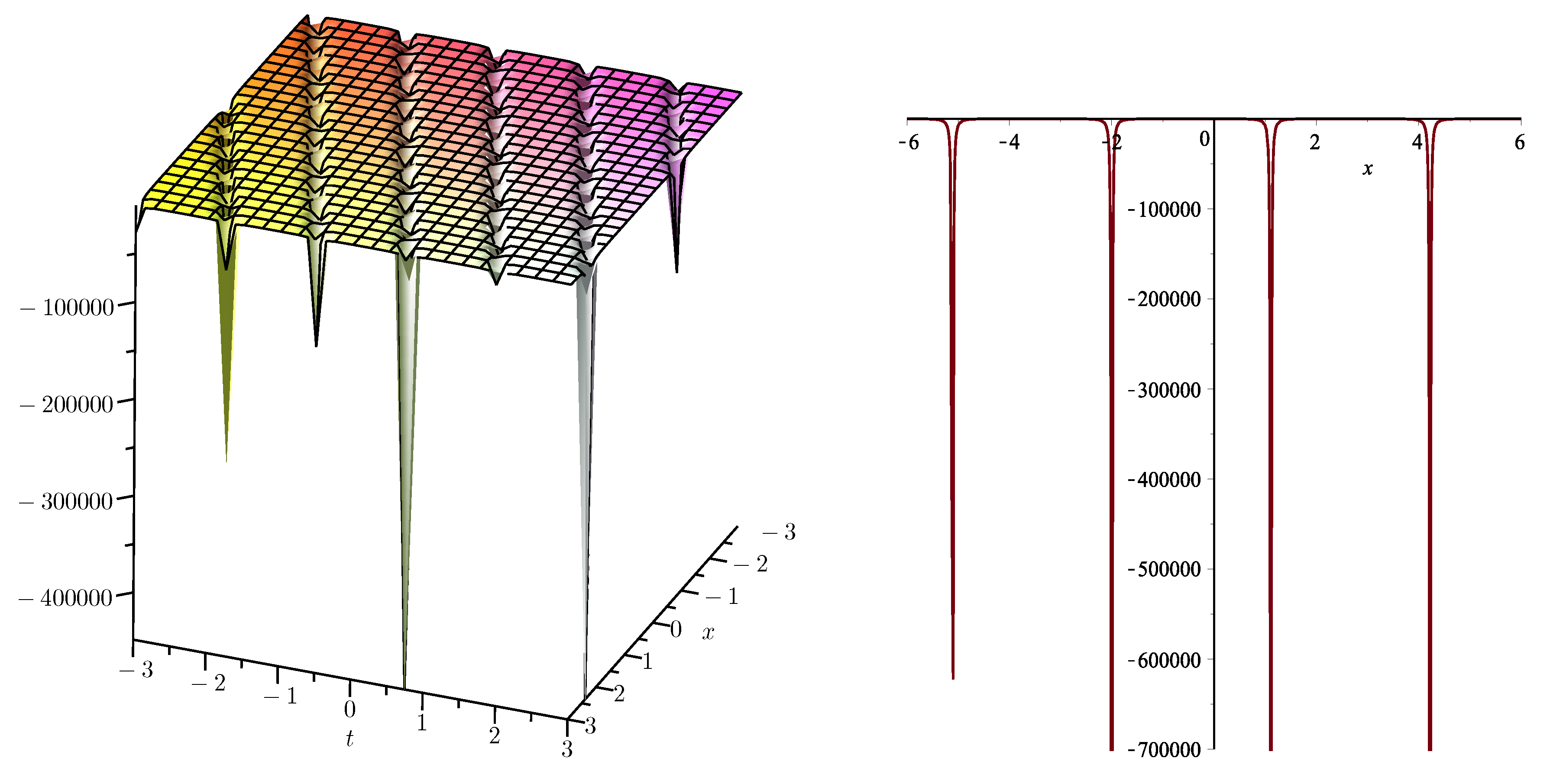
3. Solutions to the Perturbed Boussinesq Equation

Consider the following strongly PBE [44,45]

$$\begin{array}{c}\hfill q_{tt}-{\kappa }^2{q}_{xx}+p{\left(q^{2n}\right)}_{xx}+r{q}_{xxxx}=\omega q_{xx}+\rho q_{xxxx},\end{array}$$

(20)

The PBE is one of the NLEEs that the efficient shallow water wave model assists in many fields of engineering and science . To solve PBE by EHFM, we introduce following transformation

$$\begin{array}{c}\hfill q(x,t)=u\left(\xi \right),\xi =x-\nu t,\end{array}$$

(21)

Taking $n=1$ in (20) and using (21) converts PBE into the following ODE:

$$\begin{array}{c}\hfill {\nu }^2{u}^{″}-{\kappa }^2{u}^{″}+p{\left(u^2\right)}^{″}+r{u}^{⁗}=\omega u^{″}+\rho u^{⁗}.\end{array}$$

(22)

By two integrations of (22) , (22) turns into

$$\begin{array}{c}\hfill ({\nu }^2-{\kappa }^2-\omega )u+p{u}^2+(r-\rho )u^{″}=0.\end{array}$$

(23)

Using the balancing principle on (23) gives $N=2$.

Form 1: Consider that the solution of (23) in terms of (3) satisfies (4). For $N=2$, the solution to (23) has the following form:

$$\begin{array}{c}\hfill u\left(\xi \right)=a_0+a_{1}T\left(\xi \right)+a_2{T}^2\left(\xi \right),\end{array}$$

(24)

where $a_i,i=0,1,2$ are constants. By inserting (24) into (23), a system of algebraic equations is acquired. After solving obtained system of equations, we retrieve the following values of constants

$$\begin{array}{c}\hfill c=\frac{{\nu }^2-{\kappa }^2-\omega }{4(r-\rho )},a_0=\frac{-{\nu }^2+{\kappa }^2+\omega }{p},a_2=\frac{-6d(r-\rho )}{p}.\end{array}$$

(25)

By using Equations (24), (25) and (5)–(12), along with (21), we obtain the following new soliton solution of PBE:

Case 1: When $c>0$, $d>0$,

$$\begin{array}{ccc}\hfill q_1(x,t)& =& \frac{-({\nu }^2-{\kappa }^2-\omega )}{p}[1+\frac{3}{2}csc{h}^2\left(\sqrt{\frac{{\nu }^2-{\kappa }^2-\omega }{4(r-\rho )}}(\xi +{\xi }_0)\right)].\hfill \end{array}$$

(26)

Case 2: When $c<0$, $d>0$,

$$\begin{array}{ccc}\hfill q_2(x,t)& =& \frac{-({\nu }^2-{\kappa }^2-\omega )}{p}[1-\frac{3}{2}se{c}^2\left(\sqrt{\frac{-{\nu }^2+{\kappa }^2+\omega }{4(r-\rho )}}(\xi +{\xi }_0)\right)].\hfill \end{array}$$

(27)

Case 3: When $c>0$, $d<0$,

$$\begin{array}{ccc}\hfill q_3(x,t)& =& \frac{-({\nu }^2-{\kappa }^2-\omega )}{p}[1-\frac{3}{2}sec{h}^2\left(\sqrt{\frac{{\nu }^2-{\kappa }^2-\omega }{4(r-\rho )}}(\xi +{\xi }_0)\right)].\hfill \end{array}$$

(28)

Case 4: When $c<0$, $d>0$,

$$\begin{array}{ccc}\hfill q_4(x,t)& =& \frac{-({\nu }^2-{\kappa }^2-\omega )}{p}[1-\frac{3}{2}cs{c}^2\left(\sqrt{\frac{-{\nu }^2+{\kappa }^2+\omega }{4(r-\rho )}}(\xi +{\xi }_0)\right)].\hfill \end{array}$$

(29)

Case 5: When $c>0$, $d=0$,

$$\begin{array}{ccc}\hfill q_5(x,t)& =& \frac{-({\nu }^2-{\kappa }^2-\omega )}{p}.\hfill \end{array}$$

(30)

Case 6: When $c<0$, $d=0$,

$$\begin{array}{ccc}\hfill q_6(x,t)& =& \frac{-({\nu }^2-{\kappa }^2-\omega )}{p}.\hfill \end{array}$$

(31)

Case 7: When $c=0$, $d>0$,

$$\begin{array}{ccc}\hfill q_7(x,t)& =& \frac{-({\nu }^2-{\kappa }^2-\omega )}{p}-\frac{6(r-\rho )}{p{(\xi +{\xi }_0)}^2}.\hfill \end{array}$$

(32)

Case 8: When $c=0$, $d<0$,

$$\begin{array}{ccc}\hfill q_8(x,t)& =& \frac{-({\nu }^2-{\kappa }^2-\omega )}{p}-\frac{6(r-\rho )}{p{(\xi +{\xi }_0)}^2}.\hfill \end{array}$$

(33)

Form 2: Let solution of (22) in the form of (3) satisfy (13). For $N=2$, the solution of (22) has the form

$$\begin{array}{c}\hfill u\left(\xi \right)=a_0+a_{1}T\left(\xi \right)+a_2{T}^2\left(\xi \right),\end{array}$$

(34)

where $a_i,i=0,1,2$ are constants. By inserting (23) in (22), we get a system of algebraic equations. After solving the obtained system of equations, following values of constants are acquired

$$\begin{array}{c}\hfill c=\frac{-{\nu }^2+{\kappa }^2+\omega }{4d(r-\rho )},\\ \hfill a_0=\frac{{\nu }^2-{\kappa }^2-\omega }{2p},\\ \hfill a_2=\frac{-6d^2(r-\rho )}{p}.\end{array}$$

(35)

Using Equations (14)–(19), (34), and (35), along with (21), we get the following soliton solution of PBE:

Case 1: When $cd>0$,

$$\begin{array}{ccc}\hfill q_9(x,t)& =& \frac{({\nu }^2-{\kappa }^2-\omega )}{2p}-\frac{6d^2(r-\rho )}{p}\hfill \\ & \times & {\left[sgn\left(\frac{-{\nu }^2+{\kappa }^2+\omega }{4d(r-\rho )}\right)\sqrt{\frac{-{\nu }^2+{\kappa }^2+\omega }{4d^2(r-\rho )}}tan\left(\sqrt{\frac{-{\nu }^2+{\kappa }^2+\omega }{4(r-\rho )}}(\xi +{\xi }_0)\right)\right]}^2.\hfill \end{array}$$

(36)

Case 2: When $cd>0$,

$$\begin{array}{ccc}\hfill q_{10}(x,t)& =& \frac{({\nu }^2-{\kappa }^2-\omega )}{2p}-\frac{6d^2(r-\rho )}{p}\hfill \\ & \times & {[-sgn\left(\frac{-{\nu }^2+{\kappa }^2+\omega }{4d(r-\rho )}\right)\sqrt{\frac{-{\nu }^2+{\kappa }^2+\omega }{4d^2(r-\rho )}}cot\left(\sqrt{\frac{-{\nu }^2+{\kappa }^2+\omega }{4(r-\rho )}}(\xi +{\xi }_0)\right)]}^2.\hfill \end{array}$$

(37)

Case 3: When $cd<0$,

$$\begin{array}{ccc}\hfill q_{11}(x,t)& =& \frac{({\nu }^2-{\kappa }^2-\omega )}{2p}-\frac{6d^2(r-\rho )}{p}\hfill \\ & \times & {\left[sgn\left(\frac{-{\nu }^2+{\kappa }^2+\omega }{4d(r-\rho )}\right)\sqrt{\frac{{\nu }^2-{\kappa }^2-\omega }{4d^2(r-\rho )}}tanh\left(\sqrt{\frac{{\nu }^2-{\kappa }^2-\omega }{4(r-\rho )}}(\xi +{\xi }_0)\right)\right]}^2.\hfill \end{array}$$

(38)

Case 4: When $cd<0$,

$$\begin{array}{ccc}\hfill q_{12}(x,t)& =& \frac{({\nu }^2-{\kappa }^2-\omega )}{2p}-\frac{6d^2(r-\rho )}{p}\hfill \\ & \times & {\left[sgn\left(\frac{-{\nu }^2+{\kappa }^2+\omega }{4d(r-\rho )}\right)\sqrt{\frac{{\nu }^2-{\kappa }^2-\omega }{4d^2(r-\rho )}}coth\left(\sqrt{\frac{{\nu }^2-{\kappa }^2-\omega }{4(r-\rho )}}(\xi +{\xi }_0)\right)\right]}^2.\hfill \end{array}$$

(39)

Case 5: When $c=0$, $d>0$,

$$\begin{array}{ccc}\hfill q_{13}(x,t)& =& \frac{({\nu }^2-{\kappa }^2-\omega )}{2p}-\frac{6(r-\rho )}{p{(\xi +{\xi }_0)}^2}.\hfill \end{array}$$

(40)

Case 6: When $c<0$, $d=0$,

$$\begin{array}{ccc}\hfill q_{14}(x,t)& =& \frac{({\nu }^2-{\kappa }^2-\omega )}{2p}-\frac{3{(-{\nu }^2+{\kappa }^2+\omega )}^2}{8p(r-\rho )}{(\xi +{\xi }_0)}^2.\hfill \end{array}$$

(41)

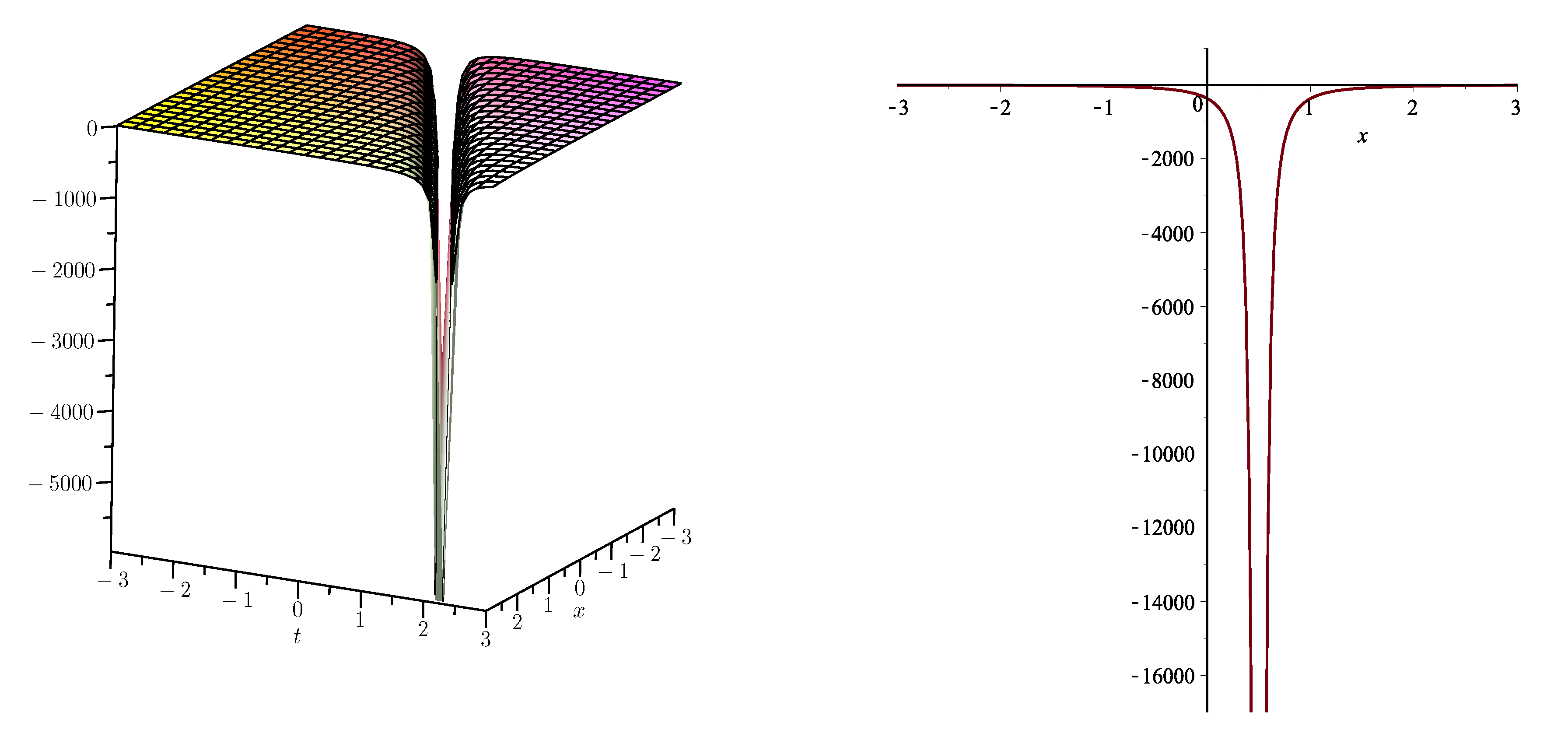
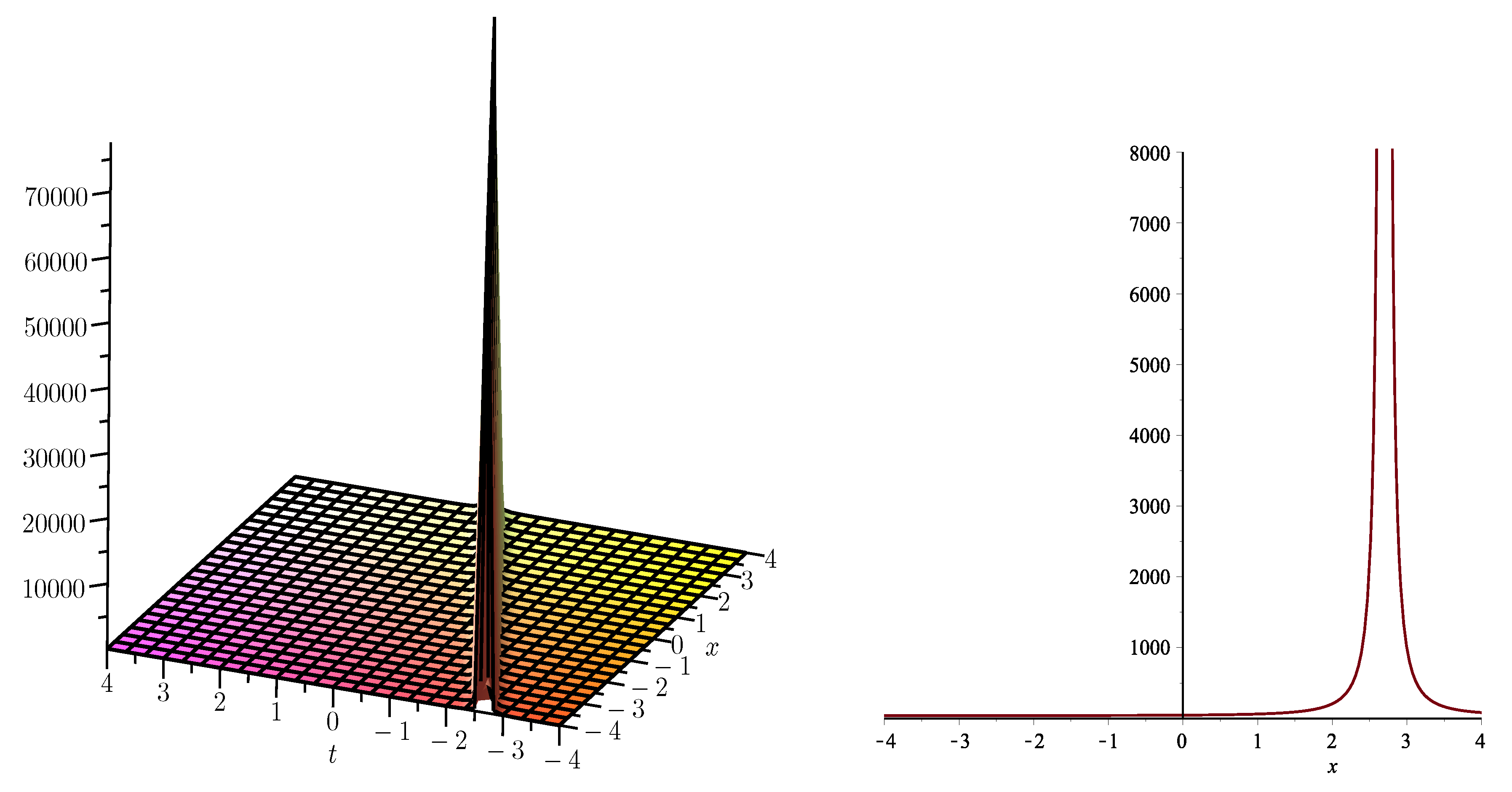
4. Solutions to the KdV–CDG Equation

Consider the combined Kdv–CDG equation [45,46]

$$\begin{array}{c}\hfill s_t+\kappa {(s_{xx}+\frac{1}{5}\alpha s^2)}_x+p{(\frac{1}{15}\alpha s^3+\alpha s{s}_{xx}+s_{xxxx})}_x=0.\end{array}$$

(42)

In order to solve combined KdV–CDG equation by EHFM, take

$$\begin{array}{c}\hfill s(x,t)=u\left(\xi \right),\xi =x-\mu t.\end{array}$$

(43)

which modifies (43) into the following ODE:

$$\begin{array}{c}\hfill -\mu u^{\prime }+\kappa {(u^{″}+\frac{1}{5}\alpha u^2)}^{\prime }+p{(\frac{1}{15}\alpha u^3+\alpha u{u}^{″}+u^{⁗})}^{\prime }=0\end{array}$$

(44)

By integrating (44), we determine

$$\begin{array}{c}\hfill -\mu u+\kappa (u^{″}+\frac{1}{5}\alpha u^2)+p(\frac{1}{15}\alpha u^3+\alpha u{u}^{″}+u^{⁗})=0\end{array}$$

(45)

Use balancing principle on (45) yields $N=2$.

Form 1: Consider that the solution of (45) has the form

$$\begin{array}{c}\hfill u\left(\xi \right)=a_0+a_{1}T\left(\xi \right)+a_2{T}^2\left(\xi \right),\end{array}$$

(46)

By inserting (46) into (45), an algebraic system of equations is obtained, from which we acquire following values of constants:

$$\begin{array}{c}\hfill a_0=\frac{20\mu }{\kappa },\\ \hfill c=-\frac{(15+\sqrt{15})\mu }{4(3+\sqrt{15})\kappa },\\ \hfill d=\frac{1}{10}\frac{(-9+\sqrt{15})a_2}{48}.\end{array}$$

(47)

Using Equations (5)–(12), (46),(47), and (43), the following new soliton solutions of combined KdV–CDG equation are derived:

Case 1: When $c>0$, $d>0$,

$$\begin{array}{ccc}\hfill s_1(x,t)& =& \frac{20\mu }{\kappa }\hfill \\ & +& a_2{[-\sqrt{\frac{-120(15+\sqrt{15})\mu }{(3+\sqrt{15})\kappa (-9+\sqrt{15})a_2}}csch\left(\sqrt{-\frac{(15+\sqrt{15})\mu }{4(3+\sqrt{15})\kappa }}(\xi +{\xi }_0)\right)]}^2.\hfill \end{array}$$

(48)

Case 2: When $c<0$, $d>0$,

$$\begin{array}{ccc}\hfill s_2(x,t)& =& \frac{20\mu }{\kappa }\hfill \\ & +& a_2{\left[\sqrt{\frac{120(15+\sqrt{15})\mu }{(3+\sqrt{15})\kappa (-9+\sqrt{15})a_2}}sec\left(\sqrt{\frac{(15+\sqrt{15})\mu }{4(3+\sqrt{15})\kappa }}(\xi +{\xi }_0)\right)\right]}^2.\hfill \end{array}$$

(49)

Case 3: When $c>0$, $d<0$,

$$\begin{array}{ccc}\hfill s_3(x,t)& =& \frac{20\mu }{\kappa }\hfill \\ & +& a_2{\left[\sqrt{\frac{120(15+\sqrt{15})\mu }{(3+\sqrt{15})\kappa (-9+\sqrt{15})a_2}}sech\left(\sqrt{-\frac{(15+\sqrt{15})\mu }{4(3+\sqrt{15})\kappa }}(\xi +{\xi }_0)\right)\right]}^2.\hfill \end{array}$$

(50)

Case 4: When $c<0$, $d>0$,

$$\begin{array}{ccc}\hfill s_4(x,t)& =& \frac{20\mu }{\kappa }\hfill \\ & +& a_2{\left[\sqrt{\frac{120(15+\sqrt{15})\mu }{(3+\sqrt{15})\kappa (-9+\sqrt{15})a_2}}csc\left(\sqrt{\frac{(15+\sqrt{15})\mu }{4(3+\sqrt{15})\kappa }}(\xi +{\xi }_0)\right)\right]}^2.\hfill \end{array}$$

(51)

Case 5: When $c>0$, $d=0$,

$$\begin{array}{ccc}\hfill s_5(x,t)& =& \frac{20\mu }{\kappa }+a_2{\left[exp\sqrt{-\frac{(15+\sqrt{15})\mu }{4(3+\sqrt{15})\kappa }}(\xi +{\xi }_0)\right]}^2.\hfill \end{array}$$

(52)

Case 6: When $c<0$, $d=0$,

$$\begin{array}{ccc}\hfill s_6(x,t)& =& \frac{20\mu }{\kappa }+a_2{[cos\sqrt{\frac{(15+\sqrt{15})\mu }{4(3+\sqrt{15})\kappa }}(\xi +{\xi }_0)+\iota sin\sqrt{\frac{(15+\sqrt{15})\mu }{4(3+\sqrt{15})\kappa }}(\xi +{\xi }_0)]}^2.\hfill \end{array}$$

(53)

Case 7: When $c=0$, $d>0$,

$$\begin{array}{ccc}\hfill s_7(x,t)& =& \frac{20\mu }{\kappa }+a_2\left[\frac{480}{(-9+\sqrt{15})a_2{(\xi +{\xi }_0)}^2}\right].\hfill \end{array}$$

(54)

Case 8: When $c=0$, $d<0$,

$$\begin{array}{ccc}\hfill s_8(x,t)& =& \frac{20\mu }{\kappa }+a_2\left[\frac{480}{(-9+\sqrt{15})a_2{(\xi +{\xi }_0)}^2}\right].\hfill \end{array}$$

(55)

Form 2: Let (45) have the solution in terms of (3) satisfying (13). For $N=2$, the solution of (45) has the form

$$\begin{array}{c}\hfill u\left(\xi \right)=a_0+a_{1}T\left(\xi \right)+a_2{T}^2\left(\xi \right),\end{array}$$

(56)

Substituting (46) into (45) and setting the coefficients of $T\left(\xi \right)$ to zero, a algebraic system of equations is extracted. After solving the system, the following values of constants are derived:

$$\begin{array}{c}\hfill a_0=\frac{-15}{4p}(\kappa +\sqrt{{\kappa }^2+4p\mu }),\\ \hfill a_2=\frac{-15}{8p{c}^2}[\mu +\frac{(\kappa +\sqrt{{\kappa }^2+4p\mu })\kappa }{2p}],\\ \hfill d=\frac{(\kappa +\sqrt{{\kappa }^2+4p\mu )}}{8pc}.\end{array}$$

(57)

Using Equations (14)–(19), (56), (57), and (43), we attain following new soliton solution of combined KdV-CDG equation:

Case 1: When $cd>0$,

$$\begin{array}{ccc}\hfill s_9& =& \frac{-15}{4p}(\kappa +\sqrt{{\kappa }^2+4p\mu })-\frac{15}{8p{c}^2}[\mu +\frac{(\kappa +\sqrt{{\kappa }^2+4p\mu })\kappa }{2p}]\hfill \\ & \times & {\left[sgn\left(c\right)\sqrt{\frac{8p{c}^2}{\kappa +\sqrt{{\kappa }^2+4p\mu }}}tan\left(\sqrt{\frac{\kappa +\sqrt{{\kappa }^2+4p\mu }}{8p}}(\xi +{\xi }_0)\right)\right]}^2.\hfill \end{array}$$

(58)

Case 2: When $cd>0$,

$$\begin{array}{ccc}\hfill s_{10}& =& \frac{-15}{4p}(\kappa +\sqrt{{\kappa }^2+4p\mu })-\frac{15}{8p{c}^2}[\mu +\frac{(\kappa +\sqrt{{\kappa }^2+4p\mu })\kappa }{2p}]\hfill \\ & \times & {[-sgn\left(c\right)\sqrt{\frac{8p{c}^2}{\kappa +\sqrt{{\kappa }^2+4p\mu }}}cot\left(\sqrt{\frac{\kappa +\sqrt{{\kappa }^2+4p\mu }}{8p}}(\xi +{\xi }_0)\right)]}^2.\hfill \end{array}$$

(59)

Case 3: When $cd<0$,

$$\begin{array}{ccc}\hfill s_{11}& =& \frac{-15}{4p}(\kappa +\sqrt{{\kappa }^2+4p\mu })-\frac{15}{8p{c}^2}[\mu +\frac{(\kappa +\sqrt{{\kappa }^2+4p\mu })\kappa }{2p}]\hfill \\ & \times & {\left[sgn\left(c\right)\sqrt{\frac{-8p{c}^2}{\kappa +\sqrt{{\kappa }^2+4p\mu }}}tanh\left(\sqrt{\frac{\kappa +\sqrt{{\kappa }^2+4p\mu }}{-8p}}(\xi +{\xi }_0)\right)\right]}^2.\hfill \end{array}$$

(60)

Case 4: When $cd<0$,

$$\begin{array}{ccc}\hfill s_{12}& =& \frac{-15}{4p}(\kappa +\sqrt{{\kappa }^2+4p\mu })-\frac{15}{8p{c}^2}[\mu +\frac{(\kappa +\sqrt{{\kappa }^2+4p\mu })\kappa }{2p}]\hfill \\ & \times & {\left[sgn\left(c\right)\sqrt{\frac{-8p{c}^2}{\kappa +\sqrt{{\kappa }^2+4p\mu }}}coth\left(\sqrt{\frac{\kappa +\sqrt{{\kappa }^2+4p\mu }}{-8p}}(\xi +{\xi }_0)\right)\right]}^2.\hfill \end{array}$$

(61)

Case 5: When $c=0$, $d>0$,

$$\begin{array}{ccc}\hfill s_{13}& =& \frac{-15}{4p}(\kappa +\sqrt{{\kappa }^2+4p\mu })-\frac{15}{8p{c}^2}[\mu +\frac{(\kappa +\sqrt{{\kappa }^2+4p\mu })\kappa }{2p}]\hfill \\ & \times & {\left[\frac{8pc}{(\kappa +\sqrt{{\kappa }^2+4p\mu })(\xi +{\xi }_0)}\right]}^2.\hfill \end{array}$$

(62)

Case 6: When $c<0$, $d=0$,

$$\begin{array}{ccc}\hfill s_{14}& =& \frac{-15}{4p}(\kappa +\sqrt{{\kappa }^2+4p\mu })-\frac{15}{8p{c}^2}[\mu +\frac{(\kappa +\sqrt{{\kappa }^2+4p\mu })\kappa }{2p}]\hfill \\ & \times & {\left[\frac{\kappa +\sqrt{{\kappa }^2+4p\mu }}{8pc}(\xi +{\xi }_0)\right]}^2.\hfill \end{array}$$

(63)

5. Conclusions

In this work, we presented EHFM to retrieve the multiple exact soliton solutions of the PBE and KdV–CDG equations. From this integration scheme, bright, dark, singular, periodic singular, and bright-singular combo soliton solutions are retrieved. These algorithms are concise, efficient and immensely useful in further analysis of nonlinear problems. For physical understanding of the solutions, some 2D and 3D graphs of solutions (26)–(28), (32), (36), (38), (41), (50), (51), (55), and (59)–(61) are plotted in Figure 1, Figure 2, Figure 3, Figure 4, Figure 5, Figure 6, Figure 7, Figure 8, Figure 9, Figure 10, Figure 11, Figure 12 and Figure 13. Figure 1, Figure 4, Figure 10 and Figure 13 show 3D and 2D plots of singular soliton of solutions (26), (32), (55) and (61), respectively. Figure 2, Figure 5, Figure 9, and Figure 11 represent 3D and 2D plots of periodic singular soliton of solutions (27), (36), (51), and (59), respectively. Figure 3 and Figure 8 represent 3D and 2D plots of the bright soliton of solutions (28) and (50), respectively. Figure 6 and Figure 12 demonstrate 3D and 2D plots of dark soliton of solution (38), respectively.

References

1. Miah, M.M.; Ali, H.M.S.; Akbar, M.A. An investigation of abundant traveling wave solution of complex nonlinear evolution equation. Cogent Math. 2016, 3, 1277506. [Google Scholar] [CrossRef]
2. Yong, H.; Yadong, S.; Wenjum, Y. Symbolic Computation and the Extended Hyperbolic Function Method for Constructing Exact Traveling Solution of Nonlinear PDEs. J. Appl. Math. 2012, 1, 716719. [Google Scholar] [CrossRef]
3. Islam, W.; Rehman, H.U.; Younis, M. Weakly Nonlocal Single and Combined Solitons in Nonlinear Optics with Cubic quintic Nonlinearities. Nanoelectron. Optoelectron. 2017, 12, 1008–1012. [Google Scholar] [CrossRef]
4. Rehman, H.U.; Saleem, M.S.; Zubair, M.; Jafar, S.; Latif, I. Optical solitons with Biswas-Arshed model using mapping method. Optik 2019, 194, 163091. [Google Scholar] [CrossRef]
5. Rehman, H.U.; Jafar, S.; Javed, A.; Hussain, S.; Tahir, M. New optical solitons of Biswas-Arshed equation using different techniques. Optik 2020, 206, 163670. [Google Scholar] [CrossRef]
6. Younis, M.; Rehman, H.U.; Rizvi, S.T.; Mahmood, S.A. Dark and singular optical solitons perturbation with fractional temporal evolution. Superlattices Microstruct. 2017, 104, 525–531. [Google Scholar] [CrossRef]
7. Younis, M.; Rehman, H.U.; Iftikhar, M. Traveling wave solutions to some time-space nonlinear evolution equations. Appl. Math. Comput. 2014, 249, 81–88. [Google Scholar]
8. Ullah, N.; Rehman, H.U.; Imran, M.A.; Jawad, T.A. Highly dispersive optical solitons with cubic law and cubic-quintic-septic law nonlinerity. Results Phys. 2020, 17, 103021. [Google Scholar] [CrossRef]
9. Fu, T.Z.; Liu, S.K.; Shi-Da, L. A new approach to solve nonlinear wave equations. Commun. Theor. Phys. 2003, 39, 27–30. [Google Scholar]
10. Liu, S.K.; Fu, Z.T.; Liu, S.; Zhao, Q. Jacobi elliptic function expansion method and periodic wave solutions of nonlinear wave equations. Phys. Lett. A 2001, 289, 69–74. [Google Scholar] [CrossRef]
11. Yan, Y.Z. Abundant families of Jacobi elliptic function solution of the (2+1)-dimensional integrable Davey-Stewartson-type equation via a new method. Chaos Solitons Fractals 2003, 18, 299–309. [Google Scholar] [CrossRef]
12. Fan, E.G. Extended tanh-function method and its application to nonlinear equations. Phys. Lett. A 2000, 277, 212–218. [Google Scholar] [CrossRef]
13. Parkes, E.J.; Duffy, B.R. An automated tanh-function method for finding solitory wave solutions to nonlinear evolution equations. Comput. Phys. Commun. 1996, 98, 288–300. [Google Scholar] [CrossRef]
14. Yan, Y.Z. New explicit traveling wave solutions for two new integrable coupled nonlinear evolution equation. Phys. Lett. A 2001, 292, 100–106. [Google Scholar] [CrossRef]
15. Akbar, M.A.; Ali, N.H.M. Exp-function method for Duffing equation and new solutions of (2+1)-dimensional dispersive long wave equations. Program Appl. Math. 2011, 1, 30–42. [Google Scholar]
16. He, H.J.; Wu, X.H. Exp-function method for nonlinear wave equations. Chaos Solitons Fractals 2006, 30, 700–708. [Google Scholar] [CrossRef]
17. Wang, M.L.; Li, X.Z. Extended F-expansion method and periodic wave solutions for generalized Zakharov equations. Phys. Lett. A 2005, 343, 48–54. [Google Scholar] [CrossRef]
18. Wang, M.L.; Li, X.Z. Applications at F-expansion to periodic wave solutions for a new Hamiltonian amplitude equation. Chaos Solitons Fractals 2005, 24, 1257–1268. [Google Scholar] [CrossRef]
19. Wang, M.L.; Li, X.Z.; Zhang, J.L. Various exact solutions of nonlinear Schrodinger equation with two nonlinear terms. Chaos Solitons Fractals 2007, 31, 594–601. [Google Scholar] [CrossRef]
20. Wang, M.L.; Zhou, Y.B. The periodic wave solutions for the Klein-Gordon-Schrodinger equations. Phys. Lett. A 2003, 318, 84–92. [Google Scholar] [CrossRef]
21. Zhou, B.Y.; Wang, M.L.; Mian, T.D. The periodic wave solutions for a class of nonlinear partial differential equations. Phys. Lett. A 2004, 323, 77–88. [Google Scholar] [CrossRef]
22. Seadawy, A.R. Modulation instability analysis for the generalized derivative higher order nonlinear Schrodinger equation and its the bright and dark soliton solutions. J. Electromagn. Waves Appl. 2017, 31, 1353–1362. [Google Scholar] [CrossRef]
23. Guo, Y.; Lai, S. New exact solutions for an (N+1)-dimensional generalized Boussinesq equation. Nonlinear Anal. Theory Method Appl. 2010, 72, 2863–2873. [Google Scholar] [CrossRef]
24. Guo, Y.; Wang, Y. On Weierstrass elliptic function solutions for a (N+1)-dimensional potential KdV equation. Appl. Math. Comput. 2011, 217, 8080–8092. [Google Scholar] [CrossRef]
25. Wang, M.L. Solitary wave solutions for variant Boussinesq equations. Phys. Lett. A 1995, 199, 169–172. [Google Scholar] [CrossRef]
26. Wang, M.L. Exact solutions for a compound KdV-Burgers equation. Phys. Lett. A 1996, 213, 279–287. [Google Scholar] [CrossRef]
27. Akbar, M.A.; Ali, N.H.M.; Zayed, E.M.E. Abundant exact traveling wave solutions of generalized bretherton equation via improved (G/G)-expansion method. Commun. Theor. Phys. 2012, 57, 173–178. [Google Scholar] [CrossRef]
28. Wang, M.L.; Li, X.Z.; Zhang, J.L. The (G/G)-expansion and traveling wave solutions of nonlinear evolution equations in mathematical physics. Phys. Lett. A 2008, 372, 417–423. [Google Scholar] [CrossRef]
29. Petkovir, A.J.J.M.D.; Biswas, A. Modified simple equation for nonlinear evolution equations. Appl. Math. Comput. 2010, 217, 869–877. [Google Scholar]
30. Kudryashov, N.A. Exact solutions of the generalized Kuramoto-Sivashinsky equation. Phys. Lett. A 1990, 147, 287–291. [Google Scholar] [CrossRef]
31. Zhang, Z. New exact solution to be generalized nonlinear Schrodinger equation. Fizika A 2008, 17, 125–134. [Google Scholar]
32. Khater, A.H.; Callebaut, D.K.; Helal, M.A.; Seadawy, A.R. Variational method for the nonlinear dynamic of an elliptic magnetic stagnation line. Eur. Phys. J. D 2006, 39, 237–245. [Google Scholar] [CrossRef]
33. Heal, M.A.; Seadawy, A.R. Variational method for the derivative nonlinear Schrodinger equation with computational applications. Phys. Scr. 2009, 80, 035004. [Google Scholar] [CrossRef]
34. Seadawy, A.R. Approximation solutions of derivative nonlinear Schrodinger equation with computational applications by variational method. Eur. Phys. J. Plus 2015, 130, 182. [Google Scholar] [CrossRef]
35. Li, X.Z.; Wang, M.L. A sub-ODE method for finding exact solutions of a generalized KdV-mKdV equation with high order nonlinear terms. Phys. Lett. A 2007, 361, 115–118. [Google Scholar] [CrossRef]
36. Khater, A.H.; Callebaut, D.K.; Seadawy, A.R. General soliton solutions of an n-dimentional complex Ginzburg-Landau equation, Physica Scripta. Int. J. Exp. Theor. Phys. 2000, 62, 353–357. [Google Scholar]
37. Khater, A.H.; Callebaut, D.K.; Seadawy, A.R. Nonlinear dispersive instabilities in Kelvin-Helmholtz magnetohydrodynamic flows. Phys. Scrita 2003, 67, 340–349. [Google Scholar] [CrossRef]
38. Helal, M.A.; Seadawy, A.R. Exact soliton solutions of a D-dimensional nonlinear Schrodinger terms. Zeitschrift fur Angewandte Mathematik und Physik 2011, 62, 839–847. [Google Scholar] [CrossRef]
39. Huang, Y.; Shang, Y. Thr Extended Hyperbolic Function Method for Generalized Forms of Nonlinear Heat Conducted and Huxley Equations. J. Appl. Math. 2012, 2012, 769843. [Google Scholar] [CrossRef] [Green Version]
40. Yadong, S. The Extended Hyperbolic Function Method and exact solutions of the long-short wave resonance equations. Chaos Solitons Fractals 2008, 36, 762–771. [Google Scholar]
41. Rehman, H.U.; Ullah, M.A.I.N.; Akgul, A. Exact solutions of (2+1)-dimensional Schrödinger’s hyperbolic equation using different techniques. In Numerical Methods for Partial Differential Equations; Wiley Periodicals, LLC.: Hoboken, NJ, USA, 2020. [Google Scholar] [CrossRef]
42. Yadong, S. Explicit and exact solutions for a generalized long-short wave equations with strong nonlinear term. Chaos Solitons Fractals 2005, 26, 527–539. [Google Scholar]
43. Yadong, S. Explicit and exact solutions for a class of nonlinear wave equations. Acta Math Appl. Sin. 2000, 23, 21–30. [Google Scholar]
44. Ebadi, G.; Johnson, S.; Zerrad, E.; Biswas, A. Solitons and the other non-linear waves for the perturberd Boussinesq equation with power law nonlinearity. J. King Saud Univ.-Sci. 2012, 24, 237–241. [Google Scholar] [CrossRef] [Green Version]
45. Akbar, M.A.; Ali, N.H.M.; Tanjim, T. Adequate soliton solutions to the perturbed Boussinesq equation and the KdV-Caudrey-Dodd-Gibbon equation. J. King Saud Univ.-Sci. 2020, 32, 2777–2785. [Google Scholar] [CrossRef]
46. Biswas, A.; Ebadi, G.; Triki, H.; Yildirim, A.; Yousefzadeh, N. Tolopogical soliton and other exact solutions to KdV-Caudrey-Dodd-Gibbon equation. Results Math. 2013, 63, 687–703. [Google Scholar] [CrossRef]
Figure 1. (left) 3D representation of solution (26) for ν = 1.5 , κ = 1 ,   ω = 0.5 ,   ρ = 1.5 ,   r = 1.7 ,   p = 1 ,   ξ = 2 , ξ 0 = 0.5 and 4 x ,   t 4 . (right) 2D representation of solution (26) with t = 0 and 4 x 4 ; this represents the singular soliton.
Coatings 11 01429 g001
Figure 2. (left) 3D representation of solution (27) for ν = 1.5 ,   κ = 1 ,   ω = 0.5 ,   ρ = 1.2 ,   r = 1.7 ,   p = 1 ,   ξ = 0.5 , ξ 0 = 0.5 and 3 x ,   t 3 . (right) 2D representation of solution (27) for t = 1 and 3 x 3 ; this represents the periodic singular soliton.
Coatings 11 01429 g002
Figure 3. (left) 3D representation of solution (28) for ν = 1.5 ,   κ = 1 ,   ω = 0.5 ,   ρ = 1.2 ,   r = 1.5 ,   p = 1 ,   ξ = 2.5 , ξ 0 = 2 and 5 x ,   t 5 . (right) 2D representation of solution (28) for t = 1 and 5 x 5 ; this represents the bright soliton.
Coatings 11 01429 g003
Figure 4. (left) 3D representation of solution (32) for ν = 2 ,   κ = 0.5 ,   ω = 1 ,   ρ = 0.5 ,   r = 1 ,   p = 1.5 ,   d = 1 ,   ξ = 2.5 , ξ 0 = 1.5 and 5 x ,   t 5 . (right) 2D representation of solution (32) for t = 0 and 5 x 5 ; this represents the singular soliton.
Coatings 11 01429 g004
Figure 5. (left) 3D representation of solution (36) for ν = 1.5 ,   κ = 0.5 ,   ω = 1 ,   ρ = 0 ,   r = 1.2 ,   p = 1 ,   d = 1 ,   ξ = 2 , ξ 0 = 1.5 and 4 x ,   t 4 . (right) 2D representation of solution (36) for t = 2 and 8 x 8 ; this represents the periodic singular soliton.
Coatings 11 01429 g005
Figure 6. (left) 3D representation of solution (38) for ν = 1.5 ,   κ = 0.5 ,   ω = 0 ,   ρ = 0 ,   r = 1.2 ,   p = 1 ,   d = 1 ,   ξ = 2 , ξ 0 = 1.5 and 6 x ,   t 6 . (right) 2D representation of solution (38) for t = 1 and 6 x 6 ; this represents the dark soliton.
Coatings 11 01429 g006
Figure 7. (left) 3D representation of solution (41) for ν = 0.5 ,   κ = 0 ,   ω = 1 ,   ρ = 0 ,   r = 1.5 ,   p = 1 ,   ξ = 3.7 , ξ 0 = 2 and 6 x ,   t 6 . (right) 2D representation of solution (41) for t = 1 and 6 x 6 ; this represents the kink soliton.
Coatings 11 01429 g007
Figure 8. (left) 3D representation of solution (50) for μ = 0.5 ,   κ = 0.5 ,   a 2 = 1 ,   ξ = 2 ,   ξ 0 = 0.5 and 4 x ,   t 4 . (right) 2D representation of solution (50) for t = 1 and 4 x 4 ; this represents the bright soliton.
Coatings 11 01429 g008
Figure 9. (left) 3D representation of solution (51) for μ = 1.5 ,   κ = 1 ,   a 2 = 1 ,   ξ = 2.5 , ξ 0 = 2 and 3 x ,   t 3 . (right) 2D representation of solution (51) for t = 0 and 6 x 6 ; this represents the periodic singular soliton.
Coatings 11 01429 g009
Figure 10. (left) 3D representation of solution (55) for μ = 0.5 ,   κ = 1 ,   a 2 = 1.5 ,   ξ = 2 ,   ξ 0 = 1.5 and 3 x ,   t 3 . (right) 2D representation of solution (55) for t = 1 and 3 x 3 ; this represents the singular soliton.
Coatings 11 01429 g010
Figure 11. (left) 3D representation of solution (59) for μ = 0.5 ,   κ = 0 ,   c = 1 ,   p = 1 ,   ξ = 2 ,   ξ 0 = 1.5 and 6 x ,   t 6 . (right) 2D representation of solution (59) for t = 0 and 6 x 6 ; this represents the periodic singular soliton.
Coatings 11 01429 g011
Figure 12. (left) 3D representation of solution (60) for μ = 1 ,   κ = 0 ,   c = 1 ,   p = 0.5 ,   ξ = 1.5 ,   ξ 0 = 2 and 4 x ,   t 4 . (right) 2D representation of solution (60) for t = 0 and 4 x 4 ; this represents the dark soliton.
Coatings 11 01429 g012
Figure 13. (left) 3D representation of solution (61) for μ = 1 ,   κ = 0 ,   c = 1 ,   p = 0.5 ,   ξ = 2.5 ,   ξ 0 = 2.7 and 4 x ,   t 4 . (right) 2D representation of solution (61) for t = 0 and 4 x 4 ; this represents the singular soliton.
Coatings 11 01429 g013
Publisher’s Note: MDPI stays neutral with regard to jurisdictional claims in published maps and institutional affiliations.