Mechanical Integrity of 3D Rough Surfaces during Contact


Abstract
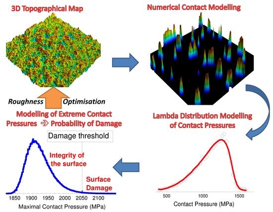
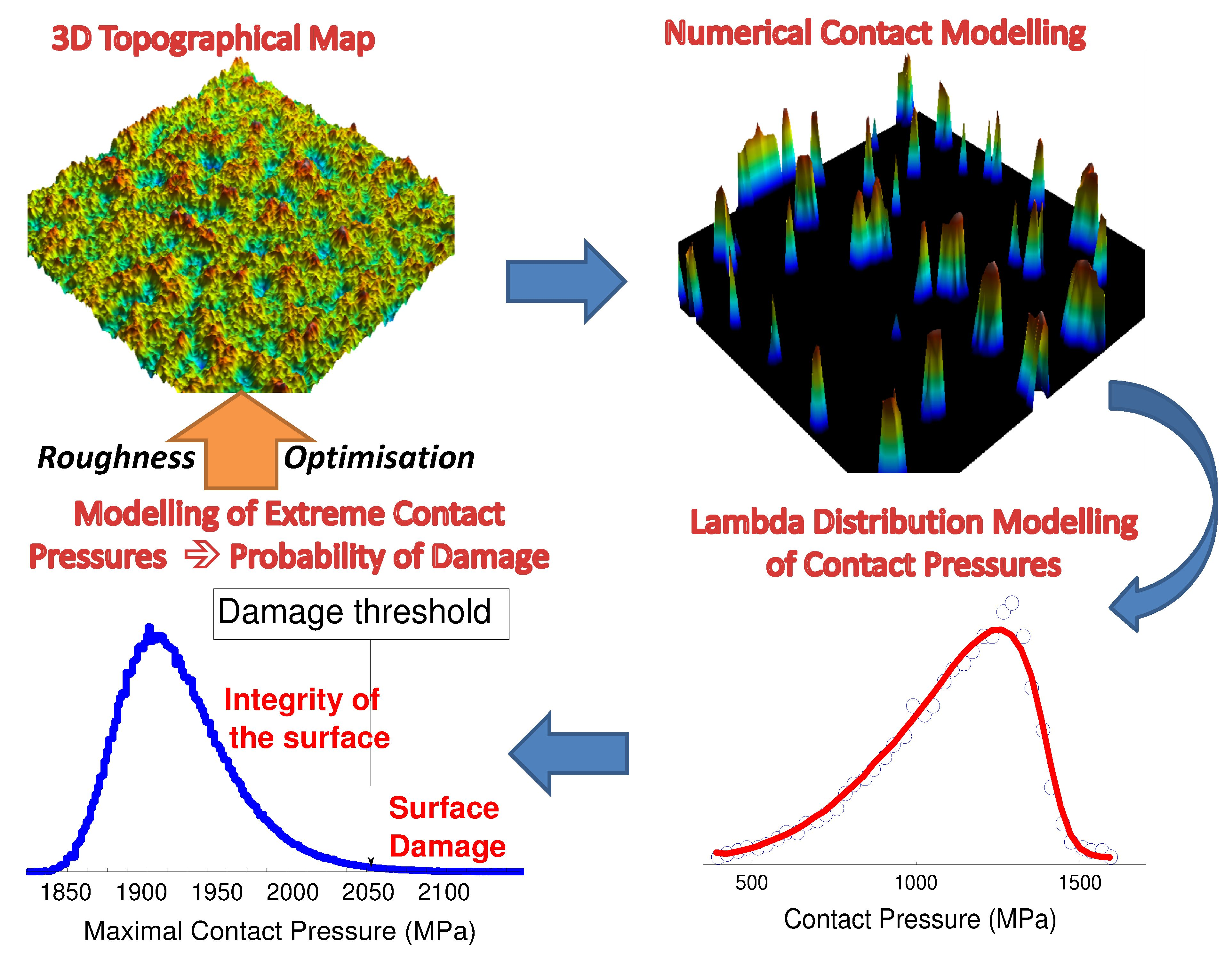
1. Introduction
2. Materials and Methods
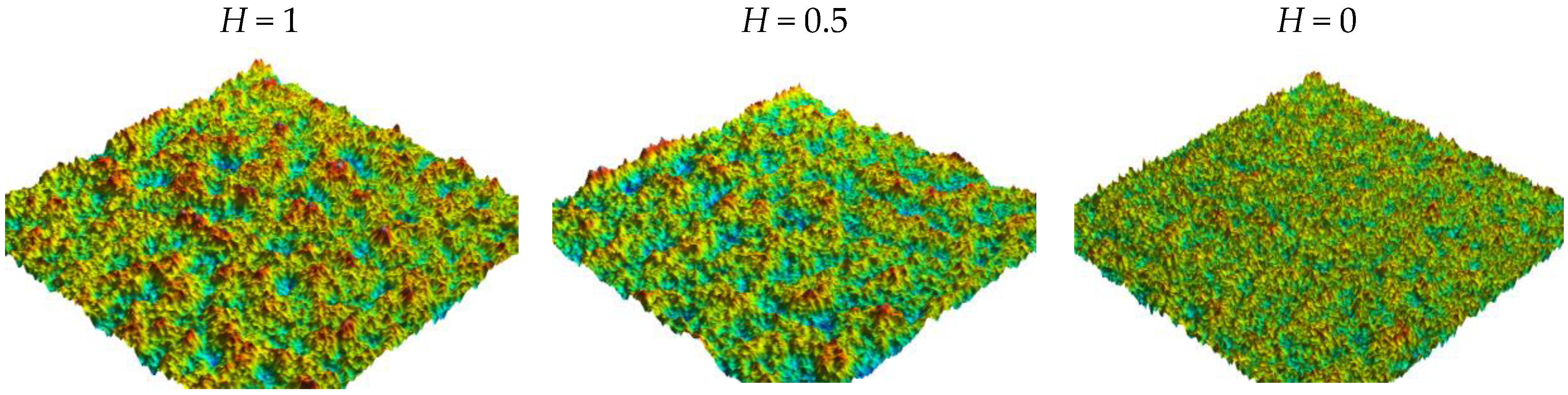
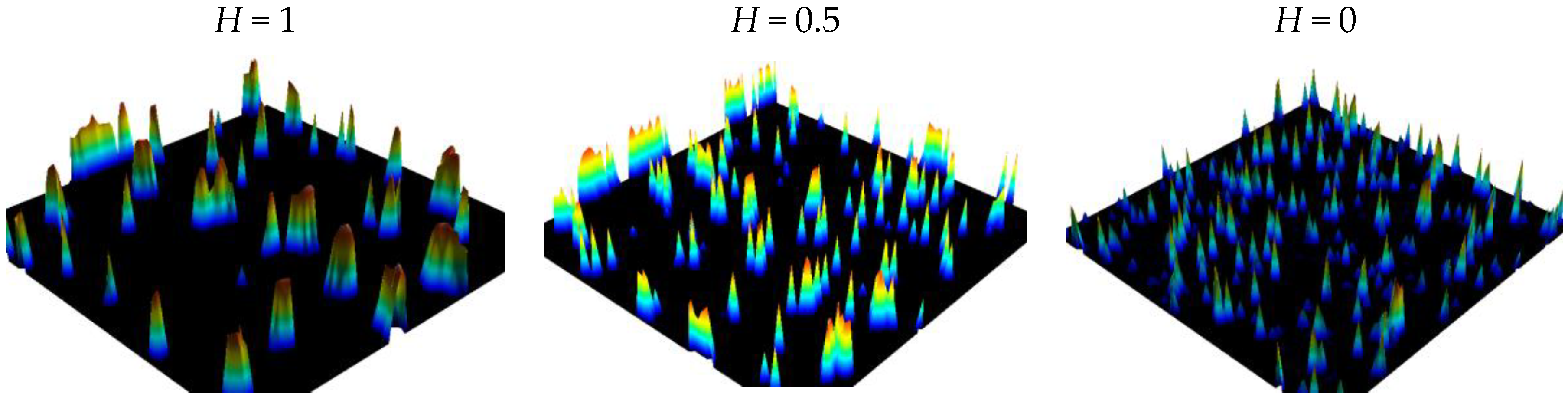
2.1. Simulation of Rough Surfaces
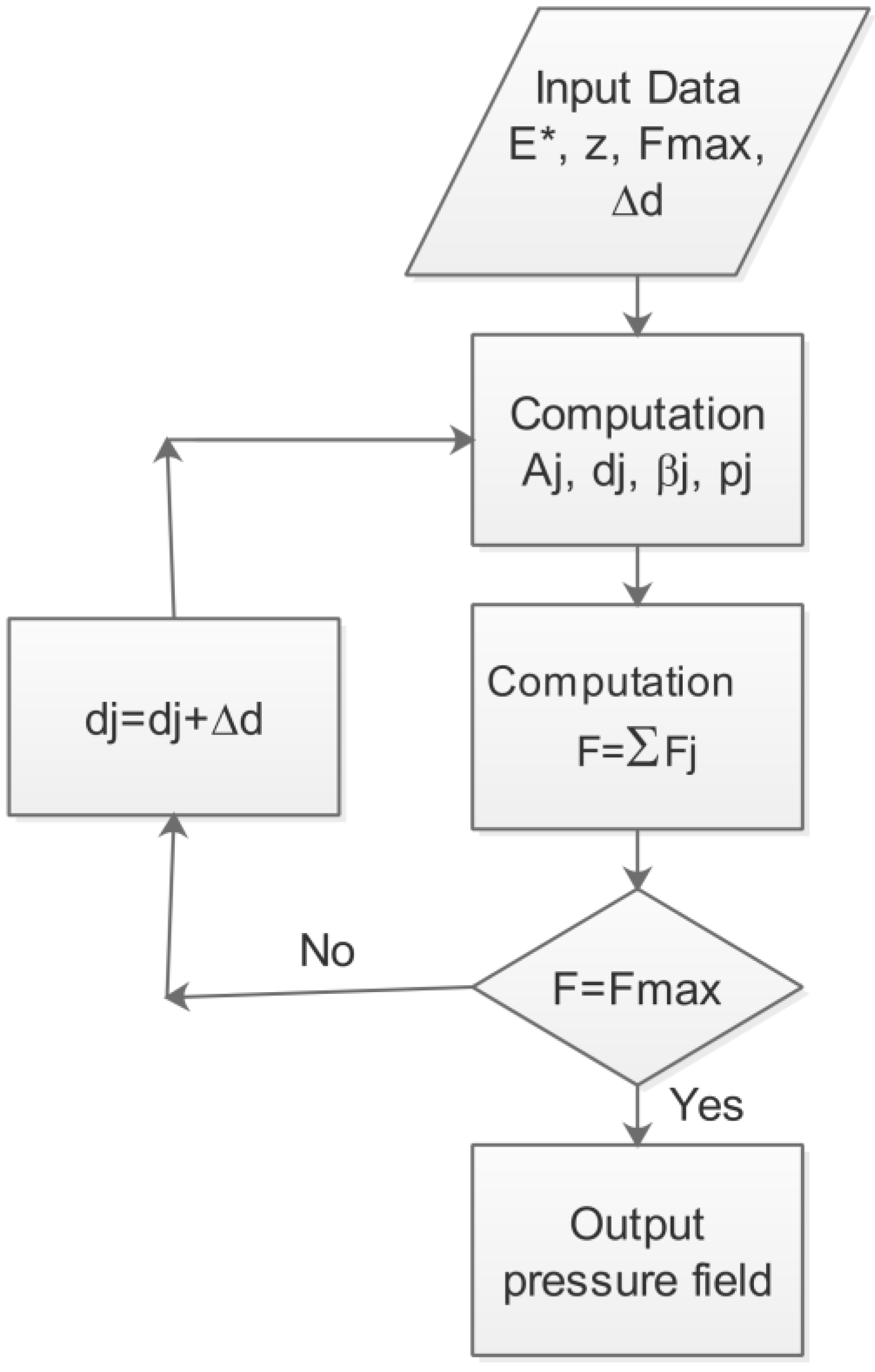
2.2. Semi-Analytical Model
2.2.1. Conical Model of Roughness
2.2.2. Solution Procedure
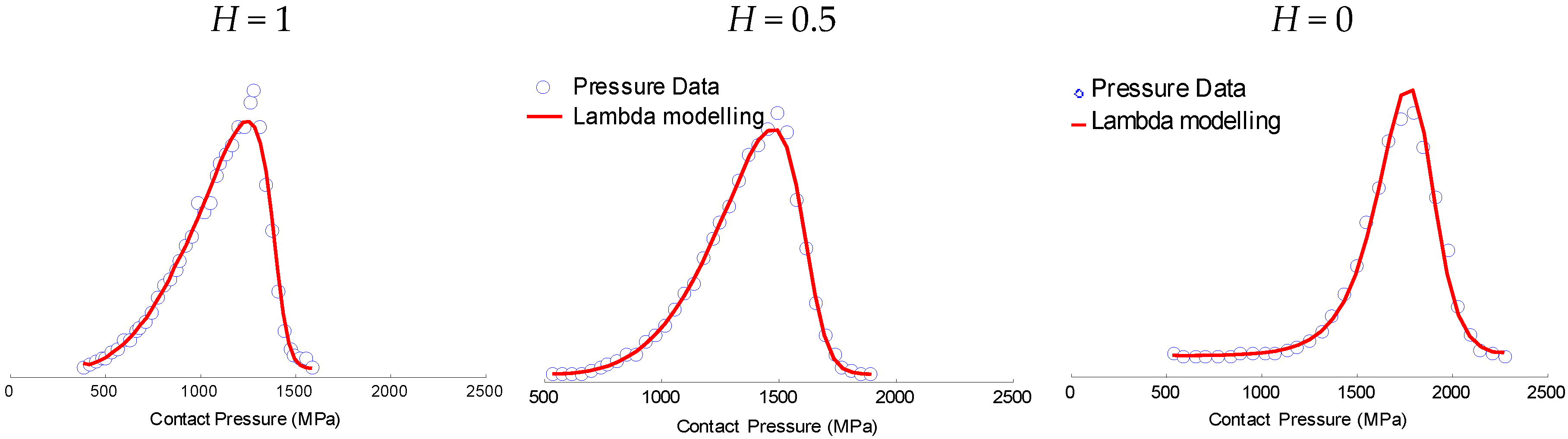
2.2.3. Pressure Distribution
3. Results
3.1. Probability Density Functions (PDFs)
3.1.1. Basic Concept
3.1.2. Numerical Estimation of Pressure PDF
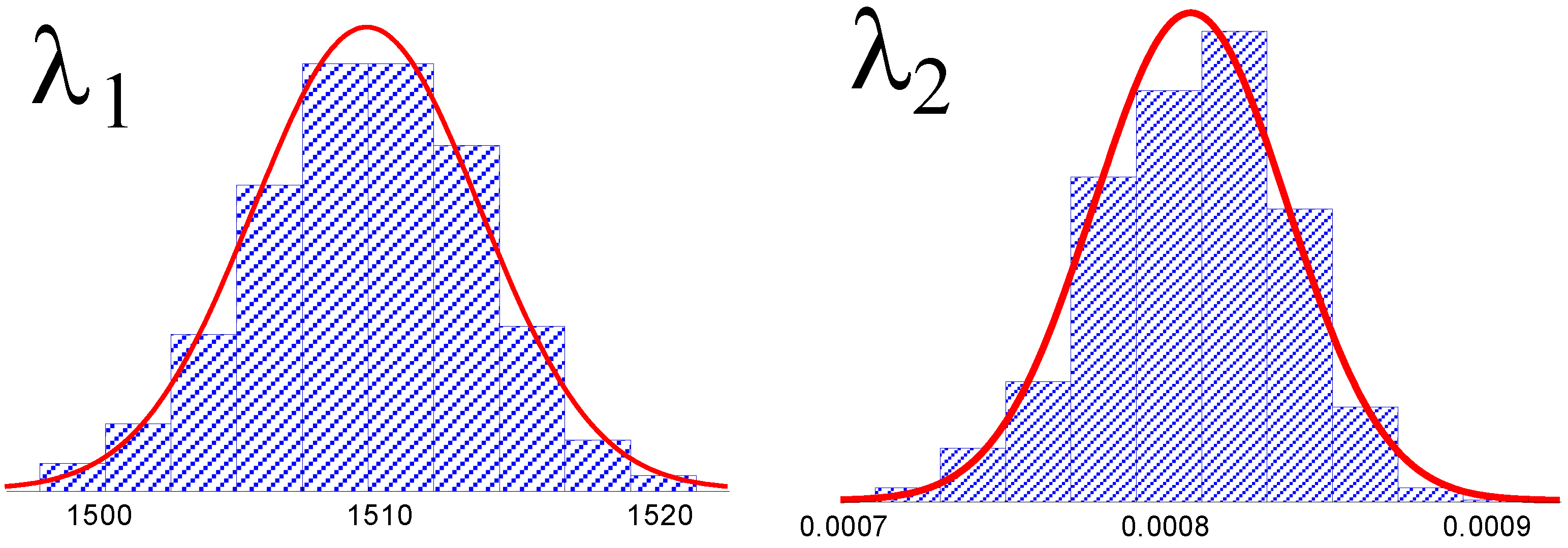
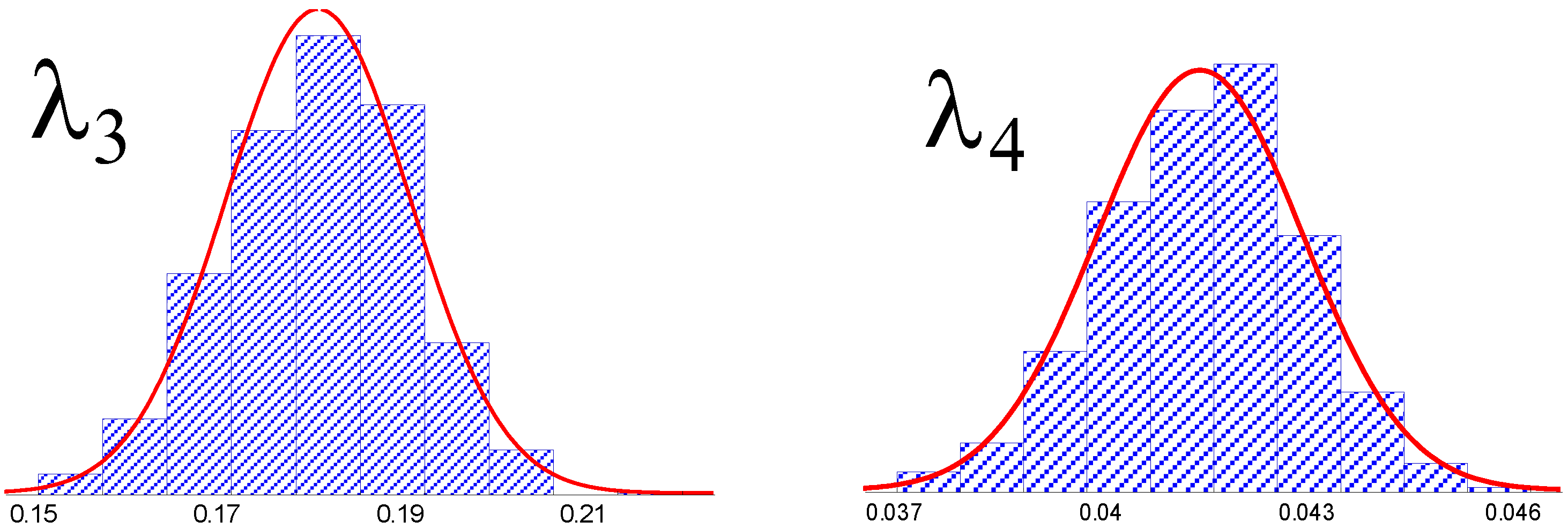
3.1.3. Bootstrap Protocol
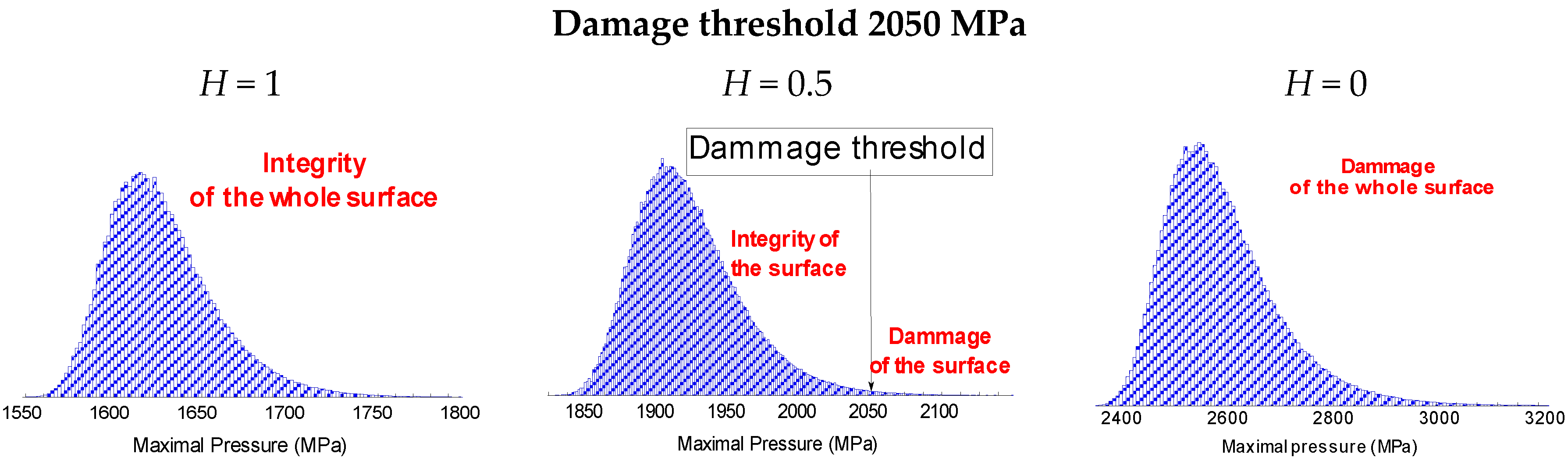
3.2. Maximal Pressure Probability Density Functions
3.2.1. Formulation
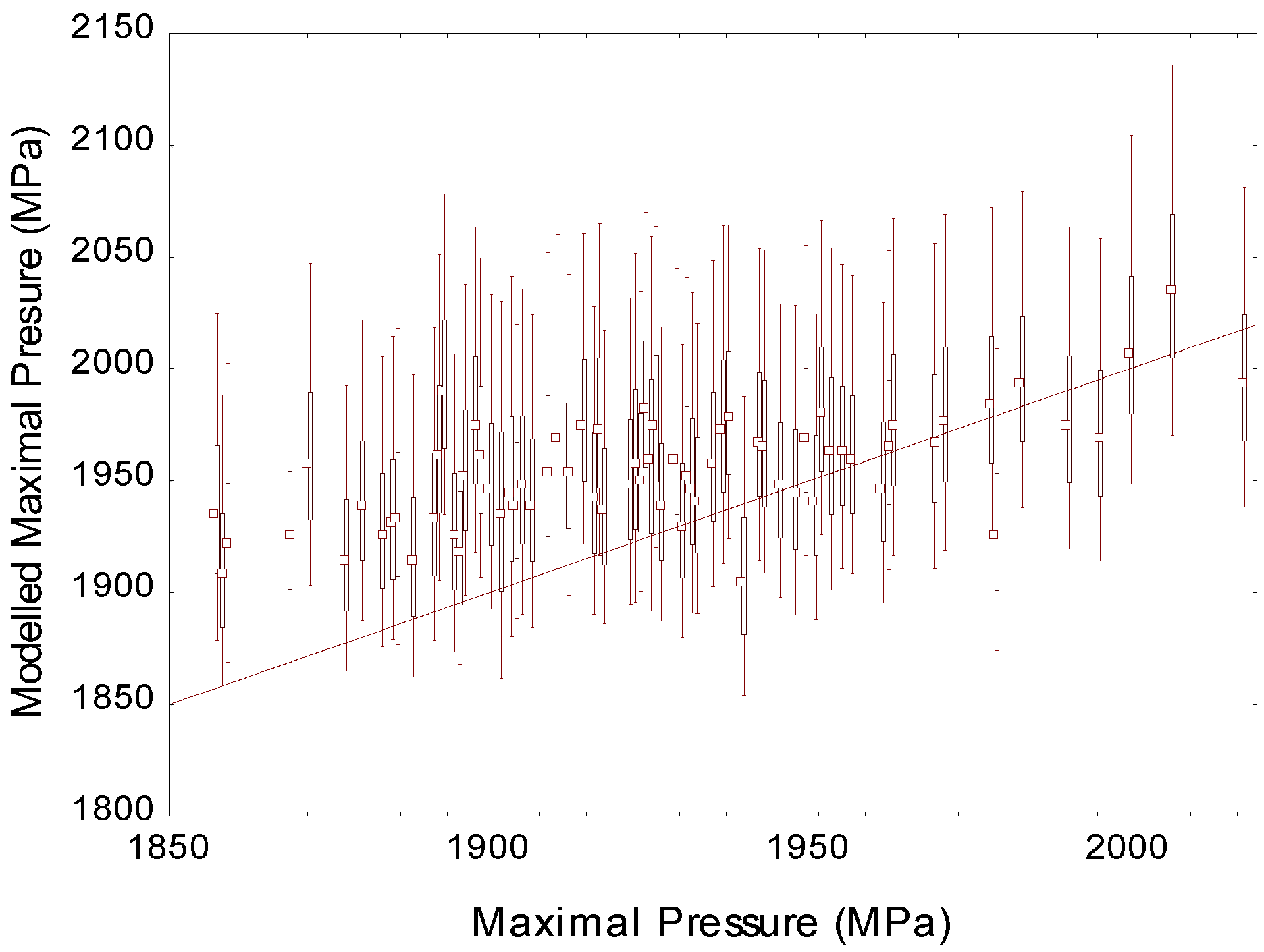
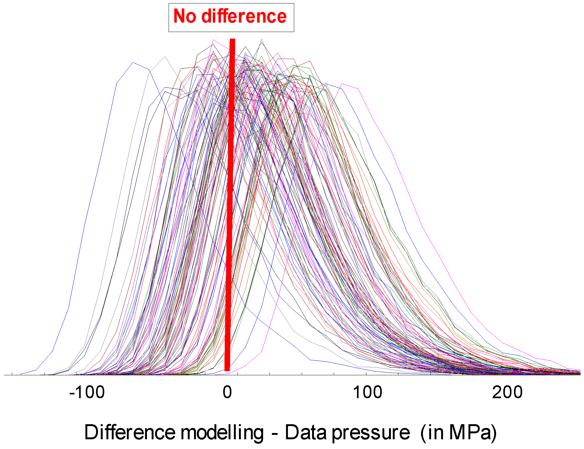
3.2.2. Numerical Validation
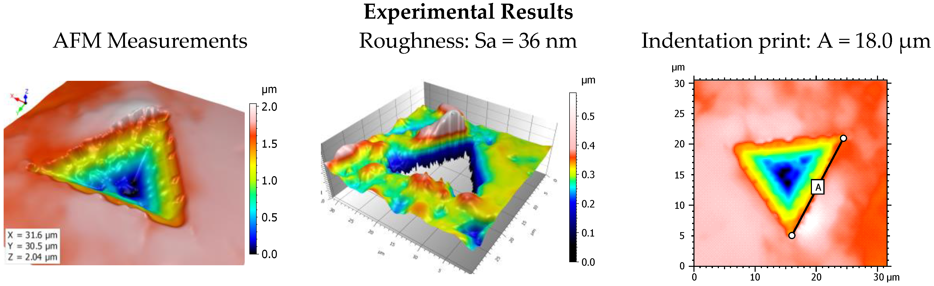
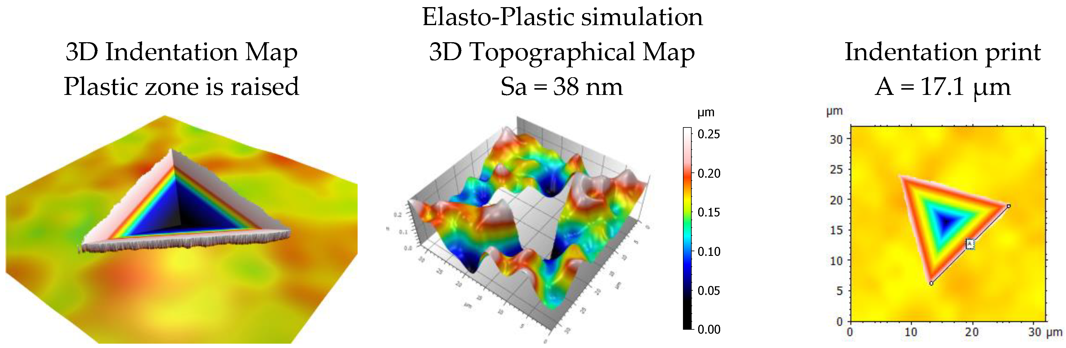
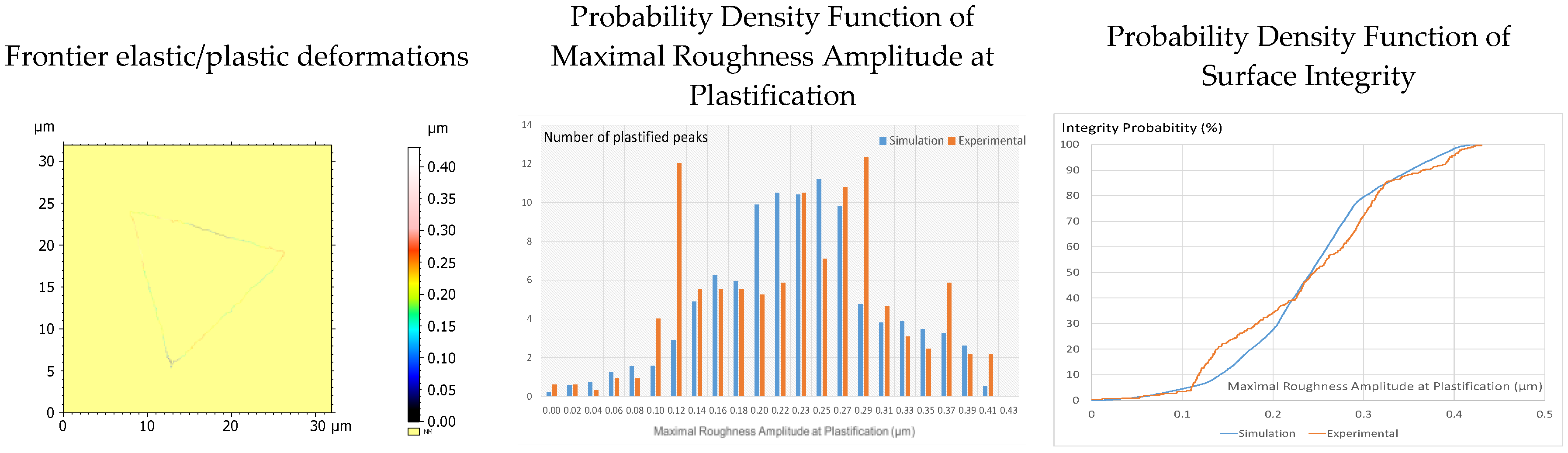
4. Experimental Validation
5. Conclusions
Author Contributions
Funding
Conflicts of Interest
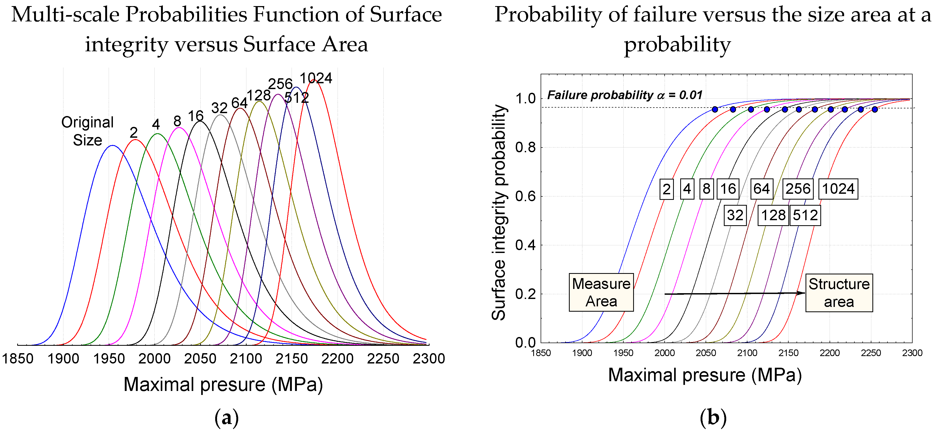
Appendix A. The MultiScale Formulation of the Probability of Failure

References
- Shen, J.; Liu, S.; Yi, K.; He, H.; Shao, J.; Fan, Z. Subsurface damage in optical substrates. Opt. Int. J. Light Electron Opt. 2005, 116, 288–294. [Google Scholar] [CrossRef]
- Fine, K.R.; Garbe, R.; Gip, T.; Nguyen, Q. Non-destructive, real time direct measurement of subsurface damage. In Proceedings of the SPIE, Orlando, FL, USA, 19 May 2005; Volume 5799, pp. 105–110. [Google Scholar]
- Stolz, C.J.; Menapace, J.A.; Schaffers, K.I.; Bibeau, C.; Thomas, M.D.; Griffin, A.J. Laser damage initiation and growth of antireflection coated S-FAP crystal surfaces prepared by pitch lap and magnetorheological finishing. In Proceedings of the SPIE, Boulder, CO, USA; 2005; Volume 5991, pp. 449–455. [Google Scholar]
- Campbell, J.H.; Hawley-Fedder, R.A.; Stolz, C.J.; Menapace, J.A.; Borden, M.R.; Whitman, P.K.; Yu, J.; Runkel, M.; Riley, M.O.; Feit, M.D.; et al. NIF optical materials and fabrication technologies: An overview. In Proceedings of the SPIE, San Jose, CA, USA, 28 May 2004; Volume 5341, pp. 84–101. [Google Scholar]
- Greenwood, J.A.; Williamson, J.P. Contact of nominally flat surfaces. In Proceedings of the Royal Society of London; Series A, Mathematical and Physical Sciences. Royal Society: London, UK, 1966; Volume 295, pp. 300–319. [Google Scholar]
- Greenwood, J.A.; Tripp, J.H. The contact of two nominally flat rough surfaces. Proc. Inst. Mech. Eng. 1970, 185, 625–633. [Google Scholar] [CrossRef]
- Tsukasa, T.; Anno, Y.; Fumio, K. Analysis of the deformation of contacting rough surface. Bull. JSME 1972, 15, 982–1003. [Google Scholar] [CrossRef]
- Van Zwol, P.J.; Svetovoy, V.B.; Palasantzas, G. Distance upon contact: Determination from roughness profile. Phys. Rev. B Condens. Matter Mater. Phys. 2009, 15, 996–1003. [Google Scholar] [CrossRef]
- Broer, W.; Palasantzas, G.; Knoester, J.; Svetovoy, V.B. Roughness correction to the Casimir force at short separations: Contact distance and extreme value statistics. Phys. Rev. B Condens. Matter Mater. Phys. 2012, 85, 155410. [Google Scholar] [CrossRef]
- Ponthus, N.; Scheibert, J.; Thøgersen, K.; Malthe-Sørenssen, A.; Perret-Liaudet, J. Statistics of the separation between sliding rigid rough surfaces: Simulations and extreme value theory approach. Phys. Rev. E 2019, 99, 023004. [Google Scholar] [CrossRef] [PubMed]
- Malekan, A.; Rouhani, S. Model of contact friction based on extreme value statistics. Friction 2019, 7, 327–339. [Google Scholar] [CrossRef]
- Bigerelle, M.; Najjar, D.; Iost, A. Multiscale functional analysis of wear: A fractal model of the grinding process. Wear 2005, 258, 232–239. [Google Scholar] [CrossRef][Green Version]
- Bhushan, B.; Majumdar, A. Elastic-plastic contact model for bifractal surfaces. Wear 1992, 153, 53–64. [Google Scholar] [CrossRef]
- Lopez, J.; Hansali, G.; Le Bossa, J.C.; Mathia, T. Caractérisation fractale de la rugosité tridimensionnelle d’une surface. J. Phys. III 1994, 4, 2501–2519. [Google Scholar] [CrossRef]
- Jourani, A.; Dursapt, M.; Hamdi, H.; Rech, J.; Zahouani, H. Effect of the belt grinding on the surface texture: Modeling of the contact and abrasive. Wear 2005, 259, 1137–1143. [Google Scholar] [CrossRef]
- Johnson, K.L. Contact Mechanics; Cambridge University Press: Cambridge, UK, 1985. [Google Scholar]
- Jourani, A.; Bigerelle, M.; Petit, L.; Zahouani, H. Local coefficient of friction, sub-surface stresses and temperature distribution during sliding contact. Int. J. Mater. Prod. Technol. 2010, 38, 44–56. [Google Scholar] [CrossRef]
- Jourani, A.; Hagege, B.; Bouvier, S.; Bigerelle, M.; Zahouani, H. Influence of abrasive grain geometry on friction coefficient and wear rate in belt finishing. Tribol. Int. 2013, 59, 30–37. [Google Scholar] [CrossRef]
- Gumbel, E.J. Statistical Theory of Extreme Values and Some Practical Applications; Applied Mathematics; National Bureau of Standards: Washington, DC, USA, 1954.
- Karian, Z.A.; Dudewicz, E.J. Fitting Statistical Distributions: The Generalized Lambda Distribution and Generalized Bootstrap Methods; Chapman & Hall: London, UK; CRC Press: Boca Raton, FL, USA, 2000. [Google Scholar]
- Karian, Z.A.; Dudewicz, E.J. Handbook of Fitting Statistical Distributions with R; Chapman & Hall: London, UK; CRC Press: Boca Raton, FL, USA, 2010. [Google Scholar]
- Najjar, D.; Bigerelle, M.; Lefebvre, C.; Iost, A. A new approach to predict the pit depth extreme value of a localized corrosion process. ISIJ Int. 2003, 43, 720–725. [Google Scholar] [CrossRef]
- Bigerelle, M.; Najjar, D.; Fournier, B.; Rupin, N.; Iost, A. Application of lambda distributions and bootstrap analysis to the prediction of fatigue lifetime and confidence intervals. Int. J. Fatigue 2006, 28, 223–236. [Google Scholar] [CrossRef][Green Version]
- Bigerelle, M.; Gautier, A.; Iost, A. Roughness characteristic length scales of micro-machined surfaces: A multi-scale modeling. Sens. Actuators B Chem. 2007, 126, 126–137. [Google Scholar] [CrossRef]
- Fournier, B.; Rupin, N.; Bigerelle, M.; Najjar, D.; Iost, A.; Wilcox, R. Estimating the parameters of a generalized lambda distribution. Comput. Stat. Data Anal. 2007, 51, 2813–2835. [Google Scholar] [CrossRef]
- Fournier, B.; Rupin, N.; Bigerelle, M.; Najjar, D.; Iost, A. Application of the generalized lambda distributions in a statistical process control methodology. J. Process Control 2006, 16, 1087–1098. [Google Scholar] [CrossRef]
- Efron, B. Bootstrap methods: Another look at the Jackknife. Ann. Stat. 1979, 7, 1–26. [Google Scholar] [CrossRef]
- Efron, B.; Tibshirani, R. An Introduction to the Bootstrap; Chapman & Hall: New York, NY, USA, 1993. [Google Scholar]
- Bowden, F.P.; Tabor, D. The Friction and Lubrication of Solids; Oxford University Press: Oxford, UK, 2001. [Google Scholar]


| Moments | GLD Parameters | |||||||
|---|---|---|---|---|---|---|---|---|
| H | λ1 | λ2 | λ3 | λ4 | ||||
| 1 | 1108 | 213 | 0.687 | 3.03 | 1307 | 9.2.10−4 | 0.276 | 0.032 |
| 0.5 | 1369 | 199 | 0.702 | 3.41 | 1509 | 8.1.10−4 | 0.181 | 0.041 |
| 0 | 1724 | 193 | 0.874 | 5.62 | 1789 | 2.6.10−4 | −0.018 | −0.034 |
© 2019 by the authors. Licensee MDPI, Basel, Switzerland. This article is an open access article distributed under the terms and conditions of the Creative Commons Attribution (CC BY) license (http://creativecommons.org/licenses/by/4.0/).
Share and Cite
Bigerelle, M.; Plouraboue, F.; Robache, F.; Jourani, A.; Fabre, A. Mechanical Integrity of 3D Rough Surfaces during Contact. Coatings 2020, 10, 15. https://doi.org/10.3390/coatings10010015
Bigerelle M, Plouraboue F, Robache F, Jourani A, Fabre A. Mechanical Integrity of 3D Rough Surfaces during Contact. Coatings. 2020; 10(1):15. https://doi.org/10.3390/coatings10010015
Chicago/Turabian StyleBigerelle, Maxence, Franck Plouraboue, Frederic Robache, Abdeljalil Jourani, and Agnes Fabre. 2020. "Mechanical Integrity of 3D Rough Surfaces during Contact" Coatings 10, no. 1: 15. https://doi.org/10.3390/coatings10010015
APA StyleBigerelle, M., Plouraboue, F., Robache, F., Jourani, A., & Fabre, A. (2020). Mechanical Integrity of 3D Rough Surfaces during Contact. Coatings, 10(1), 15. https://doi.org/10.3390/coatings10010015