Article

Smart and Rapid Design of Nanophotonic Structures by an Adaptive and Regularized Deep Neural Network

1
Shenzhen Key Laboratory of Semiconductor Lasers, School of Science and Engineering, The Chinese University of Hong Kong, Shenzhen 518172, China
2
The Future Network of Intelligence Institute (FNii), The Chinese University of Hong Kong, Shenzhen 518172, China
3
Department of Computer and Information Engineering, School of Science and Engineering, The Chinese University of Hong Kong, Shenzhen 518172, China
*
Authors to whom correspondence should be addressed.
These authors contributed equally to this work.
Nanomaterials 2022, 12(8), 1372; https://doi.org/10.3390/nano12081372
Submission received: 28 February 2022 / Revised: 8 April 2022 / Accepted: 14 April 2022 / Published: 16 April 2022

Abstract

:
The design of nanophotonic structures based on deep learning is emerging rapidly in the research community. Design methods using Deep Neural Networks (DNN) are outperforming conventional physics-based simulations performed iteratively by human experts. Here, a self-adaptive and regularized DNN based on Convolutional Neural Networks (CNNs) for the smart and fast characterization of nanophotonic structures in high-dimensional design parameter space is presented. This proposed CNN model, named LRS-RCNN, utilizes dynamic learning rate scheduling and L2 regularization techniques to overcome overfitting and speed up training convergence and is shown to surpass the performance of all previous algorithms, with the exception of two metrics where it achieves a comparable level relative to prior works. We applied the model to two challenging types of photonic structures: 2D photonic crystals (e.g., L3 nanocavity) and 1D photonic crystals (e.g., nanobeam) and results show that LRS-RCNN achieves record-high prediction accuracies, strong generalizibility, and substantially faster convergence speed compared to prior works. Although still a proof-of-concept model, the proposed smart LRS-RCNN has been proven to greatly accelerate the design of photonic crystal structures as a state-of-the-art predictor for both Q-factor and V. It can also be modified and generalized to predict any type of optical properties for designing a wide range of different nanophotonic structures. The complete dataset and code will be released to aid the development of related research endeavors.

1. Introduction

Artificial Intelligence (AI) has driven forward the development of countless research disciplines. By applying deep learning on previous data, an AI system can predict future events and make intelligent decisions at a level higher than human beings. At the frontier of deep learning, Deep Neural Networks (DNN) has demonstrated strong robustness and versatility against increasing model depth and data complexity [1,2] and has been widely applied in fields such as facial recognition [3,4] and autonomous driving [5,6]. Excitingly, recent advancement in DNN has given rise to many opportunities for the novel design of nanophotonic and optoelectronic devices, and it has been a central research thrust in the photonics community [7,8,9,10,11,12,13,14,15,16,17,18,19,20,21,22]. This is exemplified by our recent work [20], which modeled 2D photonic crystals using Convolutional Neural Networks (CNNs) and achieved very high prediction accuracies.
DNN has worked well for the following reason: A huge challenge during the design of nanophotonic structures was to correlate the design parameters (e.g., locations, radius, thickness, material selection, etc.) with optical properties (e.g., transmittance, modal volume, power, resonant wavelength, etc.). This correlation was commonly established by iterative physics-based simulations based on the researcher’s prior experience, which is both resource demanding and time consuming. Data-driven methods based on deep learning, on the other hand, can generate complex functions from mega-sized datasets and fit underlying relationships among a large number of complex parameters. Therefore, with enough training data, DNNs can capture this precise design parameter-to-optical property correlation (and its inverse) with more accuracy and little time.
Some very recent works have proposed various DNN models to characterize the relationship between design parameters and optical properties of nanophotonic structures. Ma et al. utilized a CNN model with an encode–decoder paradigm to characterize and design metasurfaces and achieved a mapping from structural pattern to reflectance [12]. Singh et al. applied fully connected (FC) layers to predict the band gap structure from given layer thicknesses of photonic topological designs [13]. Chugh et al. used fully connected layers to model waveguides and studied the relationship between their structural parameters and effective index [15]. Asano et al. applied a CNN to correlate the air hole locations with the Q-factor of a 2D photonic crystal and obtained a large Q-factor after iterative optimization [10]. Wiecha et al. adopted a CNN to model plasmonic nanostructures and was able to predict their near and far fields from an arbitrarily chosen geometry [18]. Chen et al. modeled photonic metamaterials using an Artifical Neural Network and predicted the absorbance and transmittance from given layer thicknesses [23]. Despite their demonstrated results, all the prior works have failed to address the important issue of overfitting and slow convergence speed that commonly arise in training DNNs. Moreover, most of them only have a small design parameter space and an even smaller optical property space, making their models inadequate for real-world design applications.
For this work, the authors propose a smart deep learning model for designing nanophotonic structures that is based on a self-adaptive and regularized CNN model (named LRS-RCNN by us; meaning of the acronym provided in Section 2.2). As a proof-of-concept, we applied the model to two different types of structures, 2D photonic crystals (e.g., L3 nanocavity) and 1D photonic crystals (e.g., nanobeam), both of which have been extensively studied to enhance their optical properties and are widely adopted in a variety of nanophotonic devices [10,22,24,25,26,27,28,29,30,31,32,33,34,35,36,37,38,39,40,41,42,43]. Nonetheless, the complexity of their periodic structures means that neither one is easy to design. The L3 nanocavity has been previously investigated by us using a CNN to predict only the Q-factor [20], and we adopted the same L3 design in this work. LRS-RCNN will function as an accurate predictor for both the Q-factor and modal volume V and after training, it is demonstrated that record-high prediction accuracies of both optical properties were achieved with fast convergence. Finally, LRS-RCNN was able to generalize extremely well to a fresh validation set previously unobserved by itself and still predicted Q and V with high fidelity. In summary, this generalized approach has the potential to enable the rapid design of nanoscale lasers and other nanophotonic structures with any set of optical properties.
The main merit and contributions of the proposed model are as follows:
1
To the best of our knowledge, this is the first time V is modeled by a DNN model as an optical property. V is crucial for reducing device footprints and having tight on-chip integration.
2
The employment of CNN empowers the algorithm through its unique advantage on recognizing complex patterns and extracting hidden information from images.
3
The use of learning rate scheduling (also known as adaptive learning rate) can effectively smoothen and speed up the convergence of the training process.
4
The use of L2 regularization can effectively reduce overfitting and improve the generalizibility of LRS-RCNN.
5
It has a high-dimensional design parameter (DA) space with over 160 degrees of freedom. A large DA space is a prerequisite for real-world design problems.

2. Methods

2.1. DNN Structure and Architecture

CNN is most powerful when it comes to image-related machine learning tasks [1,2,4,6,44,45]. One could argue that nanophotonic structures such as photonic crystals that seemingly are not related to images can indeed be treated as images, as extensively discussed in our prior work [20]. Thus, one can set up the learning of the optical property predictor as a CNN regression problem. Furthermore, CNN has the ability to compensate for the deficiencies of FC layers when it comes to large design parameter spaces and complex structures [9,20].
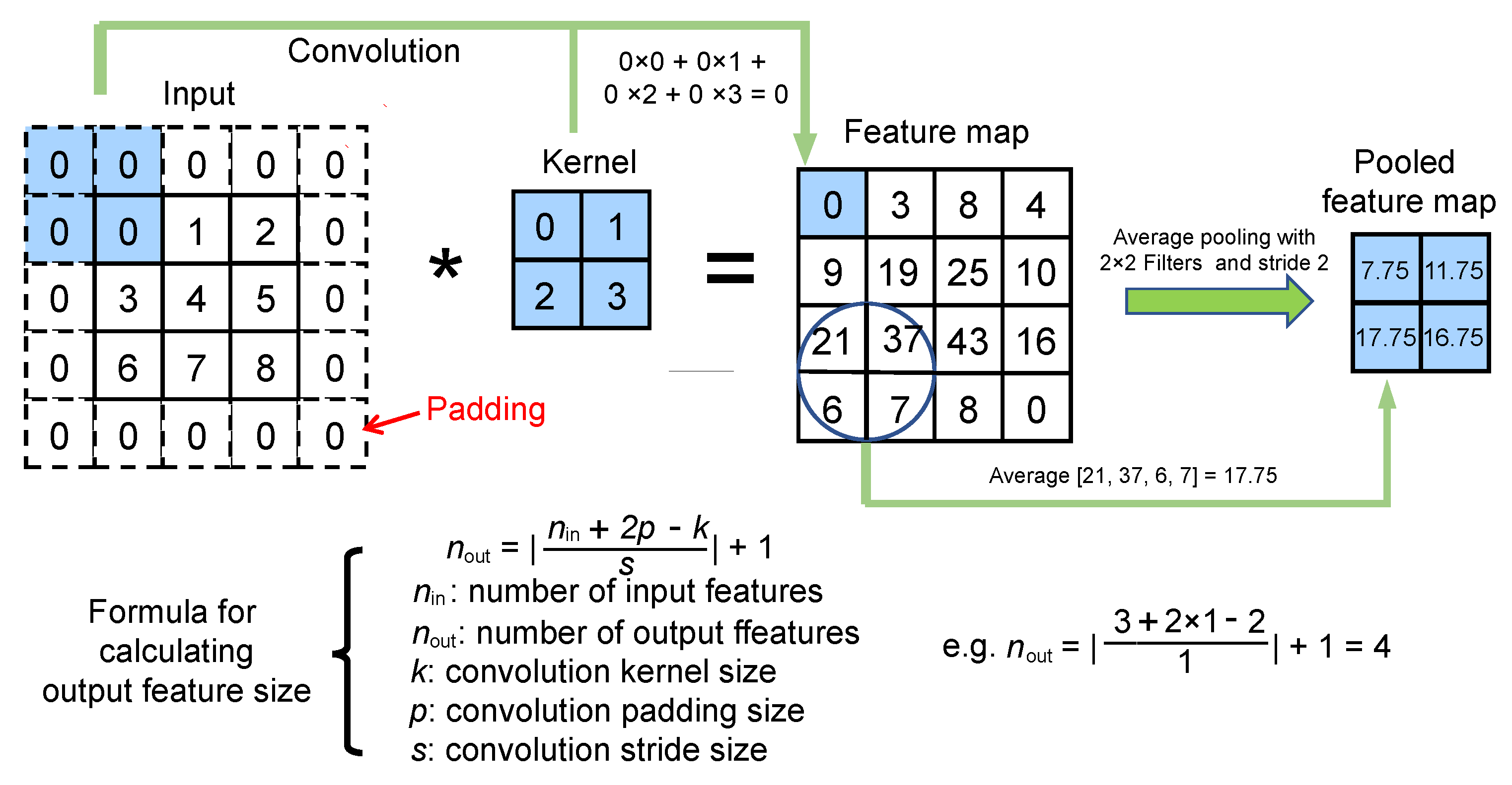
Figure 1 showcases the CNN model (i.e., LRS-RCNN) built for modeling 2D and 1D photonic crystals in this work. LRS-RCNN consists of two convolutional layers and three FC layers, with the input being a 3-channel N × 3 × H × W tensor containing user-defined design parameters and the output being an N × 2 tensor containing predicted optical properties (Q and V in our case). N represents the batch size, while H and W correspond to the height and width of the nanophotonic structure, respectively. This specific formalism allows LRS-RCNN to take in a large design parameter space of up to a few hundreds of degrees of freedom (DOF) as input. A full list of the optimized hyperparameters of LRS-RCNN is summarized in Table 1. Rectified linear unit (ReLU, f ( x ) = m a x ( 0 , x ) ) is used as it is both fast and free of vanishing/exploding gradient problems [2,46,47]. Average pooling (AP) can accelerate and stabilize the training of DNN while padding is used to preserve the size of the feature map to avoid information loss at the borders [2,47]. L2 regularization is used in backpropagation to reduce model overfitting [1,2]. Finally, an adaptive learning rate was employed to gain robustness against gradient noise and generate a smoother convergence [1,2,48]. The key working principles of CNN and average pooling are schematically illustrated in Figure 2, where the convolution formula and the feature size formula are also included.

2.2. Algorithm Description and Approach

Figure 3 schematically illustrates the full deep learning algorithm for designing nanophotonic structures by LRS-RCNN. DNNs generally need large datasets for it to effectively learn meaningful experiences and patterns that can aid in the prediction of future events. To generate a training dataset, one chooses the specific structure of interest, randomly fluctuates its design parameters (locations, radii, thicknesses, materials, refractive indices, etc.), and runs Lumerical FDTD [49] simulation to compute the corresponding optical properties (Poyting vector, Q-factor, reflectance, transmittance, resonant frequency, etc.). For our applications, we chose the target photonic crystals and generated 12,750 data samples in FDTD. A simulation of these 12,750 samples was completed in about two weeks; however, the actual time length may vary depending on the type of structures and the computing resources one possesses. We should stress that all data were strictly generated from simulations, and no experimental data/images were produced/used in this work.
After initial data collection, the algorithm follows a 3-step process, as shown in Figure 3: preprocess and split the data, train and optimize the model, and lastly validate the model. Specifically, the dataset is first normalized to have unit standard deviation and then randomly split into three sets—a training set (10,000 data points), a test set (2500 data points), and a validations set (250 data points). These three sets are randomly split up to guarantee that all data features are uniformly distributed to enhance the generalizibility of our model [2]. Normalization was necessary because the input values are on the order of 10 9 and would have led to vanishing gradients in the training process. During training, one evaluates the training results with the test dataset and closely monitors losses over entire epochs. Care should be taken to ensure the model does not overfit or underfit, both of which are undesirable cases in machine learning [1,2]. After training is complete, as the final step, one should validate the correctness of the learned model by using the validation dataset by checking for signs of any overfitting. It is important to note that the validation data should not have been seen by the model beforehand.
To realize smart and rapid design of nanophotonic structures, we utilized two important techniques that are quintessential parts of the LRS-RCNN algorithm:
1.
Adaptive learning rate through learning rate scheduling and, thus, the “LRS” in LRS-RCNN. Adaptive learning rate works by dynamically reducing the learning rate when training slows down or a metric hits a plateau and has the power of gaining robustness against gradient noise and inducing a smoother and faster convergence [1,2,48]. While there is a multitude of learning rate schedulers available, Reduce-On-Plateau was selected in this work due to its stable and consistent behavior according to our experiments.
2.
L2 Regularization and, thus, the “R” after the hyphen in LRS-RCNN. When there is a complex model with a large number of features in the dataset, L2 regularization can be used in backpropagation to address the common overfitting issue and boost generalizibility [1,2]. It works by adding a squared penalty term associated with weight parameters (W) to the loss function, as shown in Equation (1), where λ controls how much one would like to penalize large weights. The Error term corresponds to MSE in Equation (2).
R e g u l a r i z e d L o s s = E r r o r ( x i , x * ) + λ i N W i 2
Although both techniques have been rarely adopted in the literature, they have brought about tremendous benefits and improvement to the deep learning algorithm as shown later in this article.
Next, the stochastic gradient descent (SGD) optimizer was used to minimize the loss function, which is the mean squared error ( M S E ). Equation (2) calculates the M S E that is defined as the averaged distance between the value x i predicted by LRS-RCNN and the target value x * . x here could represent any optical properties associated with the chosen structure. x * is also commonly referred to as the “label” in machine learning terminology. In Equations (1) and (2), N is the batch size. An accurate predictor with low loss and fast convergence can be realized by optimizing the network hyperparameters listed in Table 1.
M S E = 1 N i N ( x i x * ) 2
Lastly, the quality of the trained LRS-RCNN will be assessed by a performance metric commonly used in deep learning: the prediction error  ϵ p r e d . ϵ p r e d represents the relative difference between x i and x * (Equation (3)). In other words, ϵ p r e d = 100 % prediction accuracy. Both Equations (2) and (3) are part of the closed-loop in Step 2 of Figure 3 for optimizing the model.
ϵ p r e d = | x i x * | x * × 100 %

3. Results and Discussion

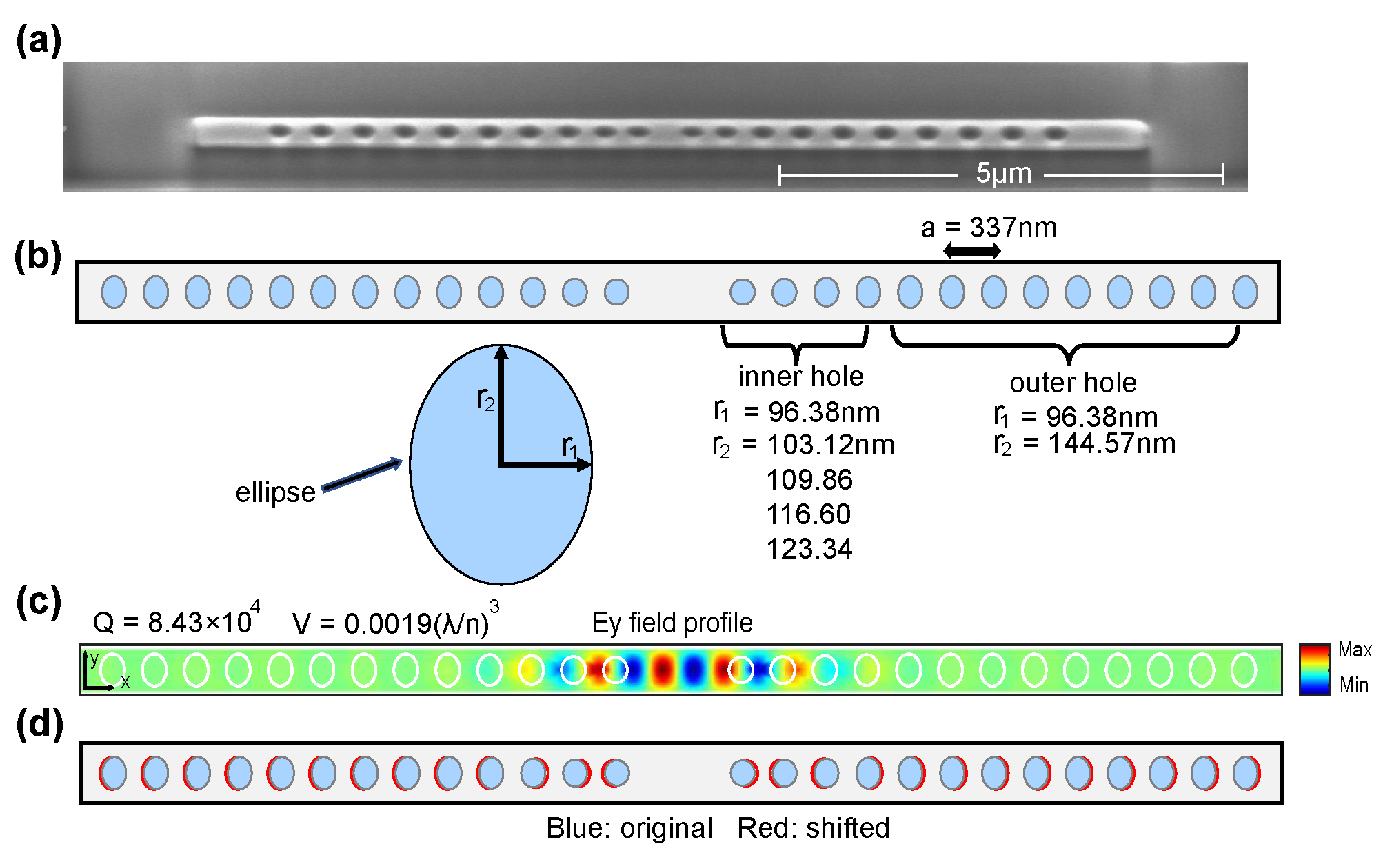
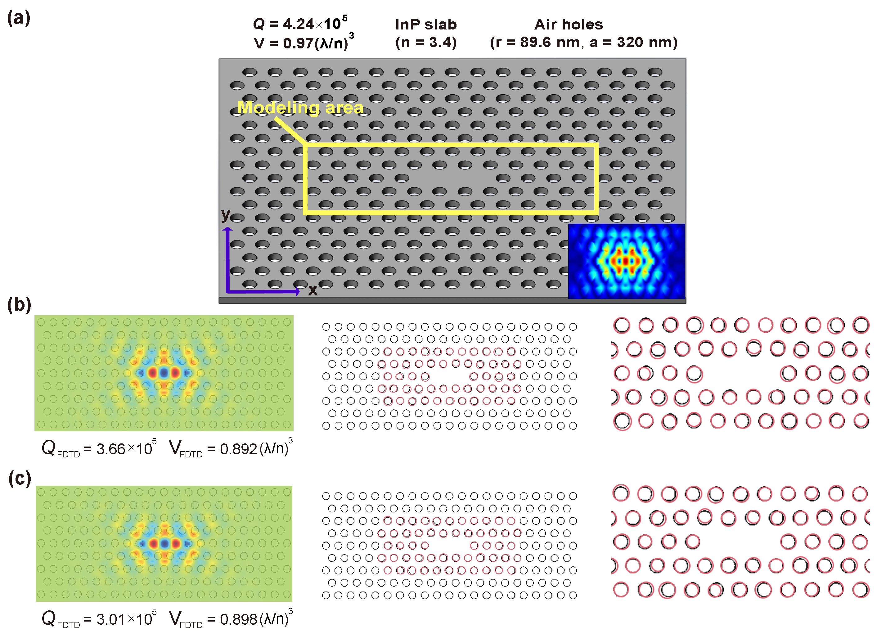
The full-fledged LRS-RCNN model, once properly trained and validated, can be applied as a smart tool to rapidly predict the optical properties of nanophotonic structures. Here, we take a nanobeam and an L3 nanocavity (Figure 4 and Figure 5, respectively) as two examples to demonstrate the power of LRS-RCNN. Figure 4 shows our initial nanobeam design similar to [36,37], where Figure 4a is the SEM image of an actual InP nanobeam fabricated by us. Figure 4b illustrates the original design parameters including semi-minor axis, semi-major axis, lattic constant a, and number of holes, while Figure 4c showcases the corresponding E y filed profile, Q-factor, and modal volume V. Figure 4d illustrates how the holes have been randomly shifted relative to Figure 4b to generate the dataset as laid out in Section 2.2. The details of the dataset generated are summarized in Table 2. Similarly to nanobeams, Figure 5 shows our initial L3 nanocavity design where Figure 5a contains the original design parameters and optical properties and Figure 5b,c are two samples in the dataset with randomly shifted holes. The L3 nanocavity dataset is also summarized in Table 2. Since nanobeam has 13 holes on each side (symmetrically shifted) and each hole has three design parameters, there is a total of 39 DOFs; by the same token, the L3 nanocavity is calculated to have 162 DOFs (the complete dataset and its detailed description can be found at [50]).

3.1. Nanobeam

Figure 6 shows the learning results of LRS-RCNN when trained to model the nanobeam. Figure 6a,b are the convergence curves of ϵ p r e d and M S E over the entire epochs for Q, respectively, while Figure 6c,d are those for V. Key performance metrics using the test dataset have been extracted from Figure 6 and summarized in Table 3 for comparison to prior works, where bold-faced numbers indicate the best metrics among all listed works. As seen in Table 3, in the case of the nanobeam, LRS-RCNN yielded dominant performance and contributed three best metrics—min ϵ p r e d for Q, min M S E , and M S E ¯ for V—that are multiple orders of magnitude smaller than existing literature data [10,13,14,15,18,22,23,51]. Furthermore, some of the other metrics, such as prediction time for a single structure and time speedup relative to conventional FDTD simulation (over six orders of magnitude), were also placed high up on the leaderboard. These results have demonstrated LRS-RCNN’s state-of-the-art capacity for the smart and rapid design of the nanobeam.
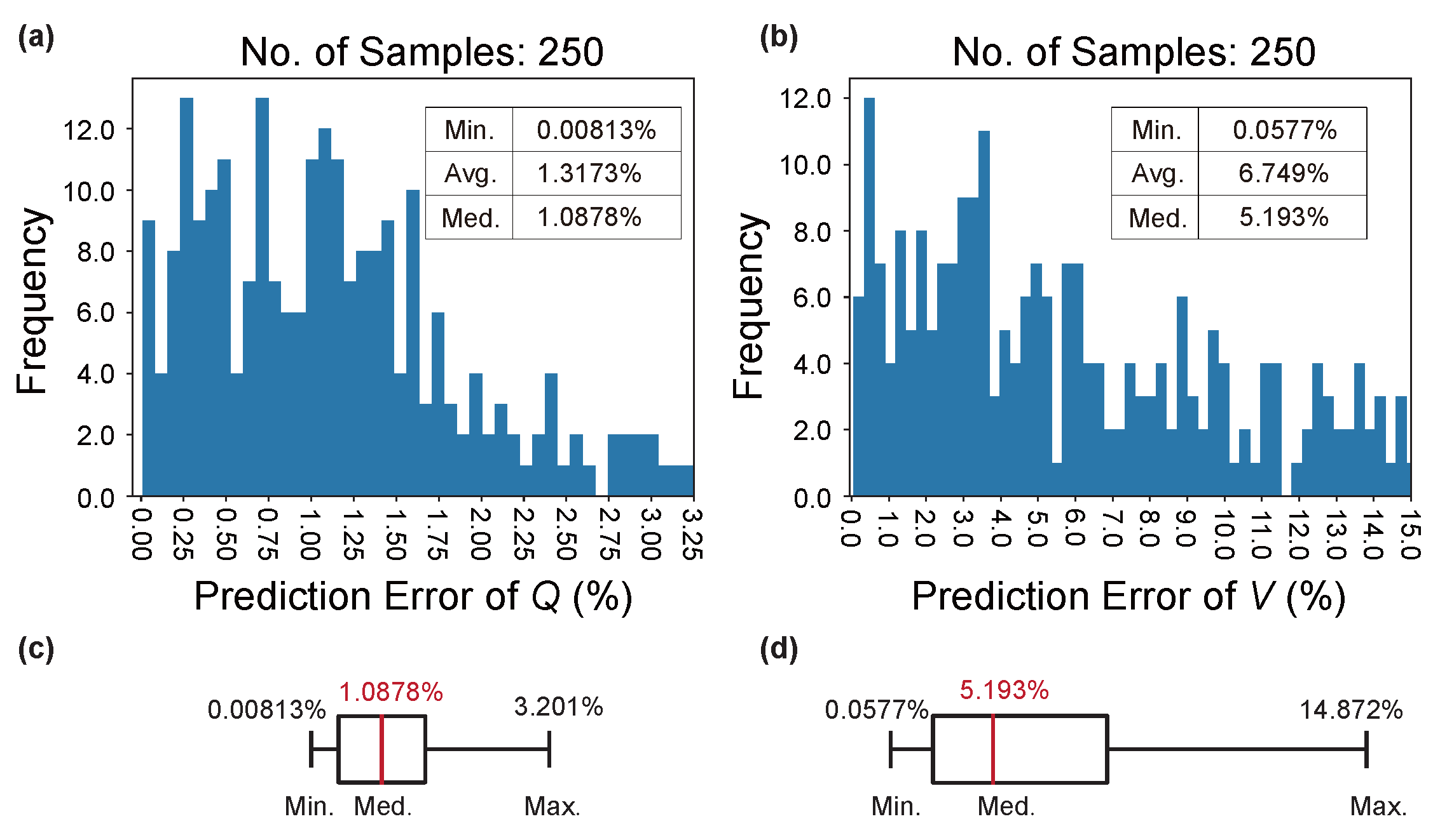
Next, Figure 7 exhibits the validation results of the trained LRS-RCNN using the validation dataset, where the prediction error ϵ p r e d for both the Q and V are plotted. This step is necessary for verifying the model’s ability to generalize unknown design parameters and for checking for any presence of overfitting. As shown in Figure 7a,c, statistically speaking, an average ϵ p r e d of 1.317% and a median ϵ p r e d of 1.088% warrant a prediction accuracy for Q close to 99% (the highest so far in the literature). Similarly, according to Figure 7b,d, the prediction accuracy for V is approaching 95%, which is still considered highly accurate for DNNs. Although the highest ϵ p r e d for V is close to 15%, it can be ignored as outliers as shown in the boxplot Figure 7d. These validation results guarantee that LRS-RCNN has attained excellent generalizibility as a predictor for both optical properties.
Lastly, it should be noted that since this is the first time V has been included in any deep learning based modeling of photonic crystals in the literature, the authors could only compare the training results of V against their own results of Q during the production of this work. The authors hope what is demonstrated here could be used as a benchmark for future work.
Table 3. Results of training LRS-RCNN with nanobeam and L3 nanocavity. Tabulated are the performance metrics of the predictor at the test/validation phase and its comparison against prior works. Data partially extracted from Figure 6 and Figure 8. Overlined parameters, such as ϵ p r e d ¯ and M S E ¯ , indicate converged values. Bold-faced numbers are best metrics. Prediction time and speedup vs. FDTD, both calculated by averaging the time measured with samples in the validation dataset, refer to the time for characterizing a single structure by LRS-RCNN. N/A means no data available from the cited work.
min ϵ p r e d ϵ p r e d ¯ min MSE MSE ¯ EpochsTraining TimePrediction TimeSpeedup (vs. FDTD)
NanobeamQ0.000157%0.0148%0.007340.007357009 min 7 × 10 5 s 5.1 × 10 6
V0.00102%0.141% 3 . 00 × 10 8 3 . 16 × 10 8
L3Q0.00105%0.0112%0.0003600.0003653005 min 9 × 10 5 s 3 × 10 6
V0.00317%0.0158%0.002520.00282
Gou et al. [22] 0.540%N/A0.000300N/A1000143 s 3 . 6 × 10 5 s 1 . 2 × 10 8
Christensen et al. [14] 0.470%0.530%N/A0.0064003 min0.02 sN/A
Asano et al. [10] 16.0%19.0%N/AN/A 2 × 10 5 N/AN/AN/A
Chugh et al. [15] 1.00%N/AN/A0.008084000N/AN/AN/A
Singh et al. [13] N/AN/A0.008100.01450045 minN/AN/A
Chen et al. [23] 0.700%5.00%N/AN/A110N/AN/AN/A
Wiecha et al. [18] N/A5.78%N/AN/A100200 min 3 × 10 3 s 10 5
Tahersima et al. [51] N/AN/AN/A0.13010,00022 minN/AN/A

3.2. L3 Nanocavity

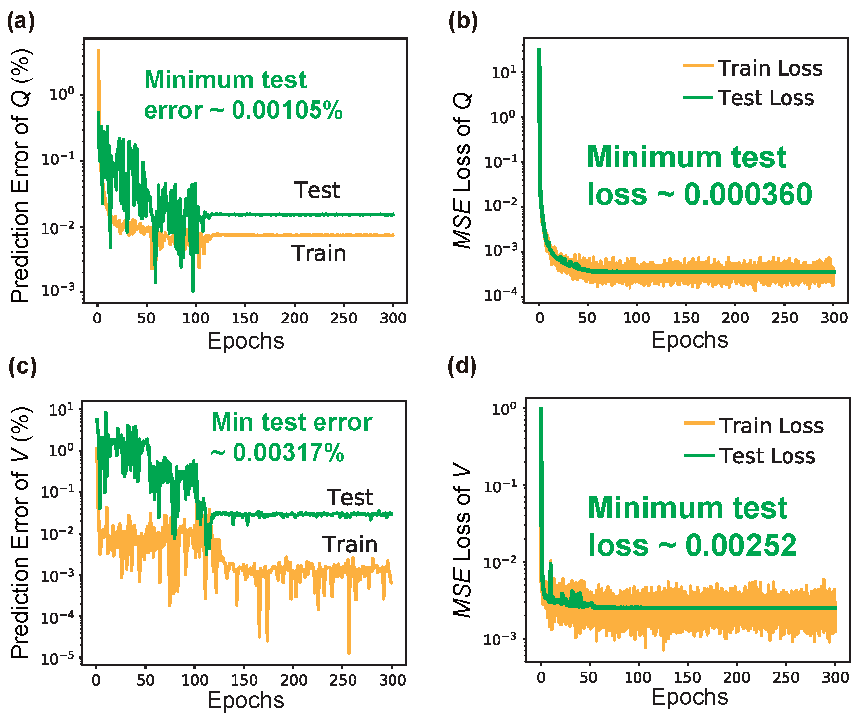
In the same fashion as the nanobeam, Figure 8 shows the learning results of LRS-RCNN when trained to model the L3 nanocavity, the metrics data of which have also been summarized in Table 3. Although LRS-RCNN only contributed one best metric (i.e., ϵ p r e d ¯ for Q), its other metrics are all ranked high on the leaderboard and are comparable to the best metrics reported for the nanobeam. For instance, the min ϵ p r e d , M S E ¯ , and prediction times are better than and/or comparable to those reported in prior works [10,13,14,15,18,22,23,51] by a large margin. Moreover, the Epochs until convergence, which include 300, leads to super fast convergence and largely reduced training time. Therefore, we have once again demonstrated the power of LRS-RCNN for the smart and rapid design of L3 nanocavities.
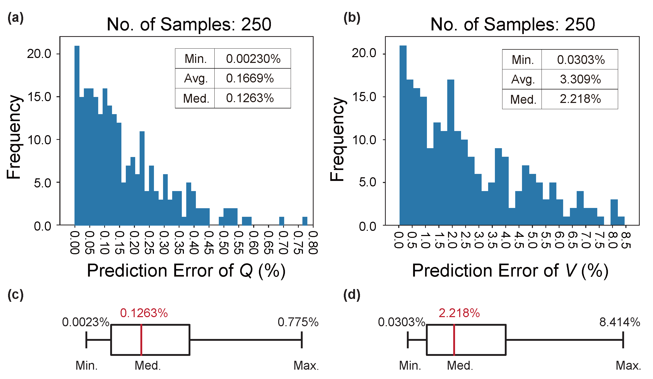
As for validation, one can see that in Figure 9a, an average ϵ p r e d of 0.167% and a median ϵ p r e d of 0.126% warrant a prediction accuracy for Q close to 99.9% (the highest so far in the literature). Similarly, according to Figure 9b, the prediction accuracy for V is approaching 97%, which is generally regarded as highly accurate for DNNs. Although the max ϵ p r e d for V is as high as 8.4%, it can be ignored as outliers as illustrated in the boxplot of Figure 9d. The validation results here can reinforce the fact that LRS-RCNN is a well generalizible predictor for unseen optical properties.

3.3. On the Importance of Adaptiveness and Regularization

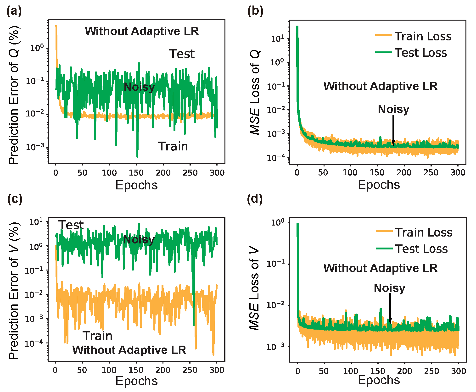
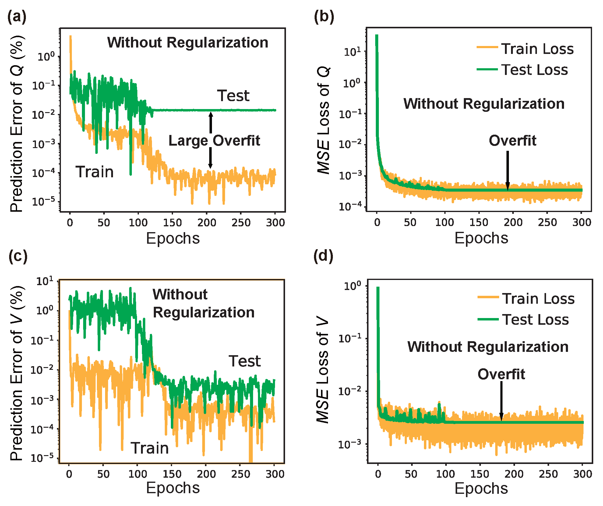
The significant impacts learning rate scheduling (LRS) and L2 regularization have on the deep learning model is discussed here. For simplicity, we only conducted experiments with L3 nanocavity, and similar results should easily extend to nanobeam and other structures. For the comparative experiment, the learning curves of LRS-RCNN without using LRS and L2 regularization are compared to those shown previously in Figure 8. It should be noted that the exact same hyperparameters and dataset are used here for training. Figure 10 shows the results without using LRS, where it can be observed that the learning curves are much more noisier than those in Figure 8 and they even failed to converge within the initial 300 epochs. This means a much slower convergence speed. Next, in Figure 11, one can observe the existence of large overfittings in all of them, but (c) when the L2 regularization is not used, which means poor generalizibility of the trained model. Therefore, we can conclude that both LRS (i.e., adaptive learning rate) and L2 regularization are crucial for the realization of smart and rapid designs.

4. Conclusions

In conclusion, this work has proposed and successfully demonstrated a self-adaptive and regularized CNN model for designing nanophotonic structures. The smart LRS-RCNN with dynamic learning rate scheduling and L2 regularization allows one to rapidly predict optical properties with high confidence from a large design parameter space. Specifically, when tested on two different photonic crystal structures, all major performance metrics improved by several orders of magnitude compared to previously reported values and, thus, proved that LRS-RCNN reached a state-of-the-art capacity. Using a validation set not previously seen, LRS-RCNN was still able to predict Q and V with an accuracy up to 99.9% and 97%, respectively. This demonstrates the strong generalizibility of the trained model that allows for the prediction of optical properties from an arbitrary set of design parameters or even arbitrary nanophotonic structures. In addition, since this is the first time V has been characterized by a deep learning model, we hope our work can serve as a benchmark for assessing related works in the future. Lastly and more broadly, this generalized accurate predictor potentially paves the way for the rapid design of a series of optoelectronic and photonic integrated devices [32,52,53,54,55,56,57,58,59,60,61] with an extremely high performance caliber.
A limitation of this work might be a lack of experimental data that back the numerical findings. However, given Lumerical FDTD’s proven strong fidelity relative to experimental data, we can say with confidence that the results in Figure 6, Figure 7, Figure 8 and Figure 9 and Table 3 are highly accurate and reliable. Nonetheless, using experiments to support calculations is still an important component of scientific research and worth our attention going forward. Efforts could further develop our architecture to predict more optical properties, including resonance frequency, full width at half maximum and lasing threshold, etc., all of which are key attributes of lasers based on photonic crystals. This would likely require the adoption of a more powerful DNN, and the latest development in vision transformers [62] and attention nets [63] are promising candidates to choose from. In addition, data collection so far takes up to two weeks to complete due to the large computational complexity of FDTD simulations. To resolve this, we would turn to some open-source light-weight simulation packages such as MPB and MEEP that would greatly reduce time consumption at the cost of losing certain degree of accuracy. Another benefit of this alternative approach would be the ability to collect more data. Furthermore, we could experiment our algorithm on a more diverse pool of structures, such as plasmonic structures, metamaterials, and DFB lasers, all of which are important and interesting paths to pursue. Lastly, instead of relying on aimlessly cascading DNNs or gradient-based optimization algorithms, we could employ the latest reinforcement learning models [64] to inverse design and optimize nanophotonic structures on a large scale.

Author Contributions

Conceptualization, Z.Z. and R.L.; methodology, R.L., Z.Z. and X.G.; software, R.L.; validation, R.L. and X.G.; formal analysis, R.L.; investigation, R.L. and X.G.; resources, Z.Z. and Z.L.; data curation, R.L. and Y.S.; writing—original draft preparation, R.L.; writing—review and editing, R.L.; visualization, Y.S. and K.L.; supervision, Z.Z. and Z.L.; project administration, R.L.; funding acquisition, Z.Z. All authors have read and agreed to the published version of the manuscript.

Funding

This work is supported by National Natural Science Foundation of China under Grant No.62174144; Shenzhen Fundamental Research Fund under Grant No.JCYJ20210324115605016 and No.JCYJ20210324120204011; Shenzhen Key Laboratory Project under Grant No.ZDSYS201603311644527; Longgang Key Laboratory Project under Grant No.ZSYS2017003 and No.LGKCZSYS2018000015; Longgang Matching Support Fund No.CXPTPT-2017-YJ-002 and No.201617486; President’s Fund (PF01000154); and the Optical Communication Core Chip Research Platform.

Institutional Review Board Statement

Not applicable.

Informed Consent Statement

Not applicable.

Data Availability Statement

The data and code presented in this study are openly available in Github at https://github.com/Arcadianlee/Deep-Learning-Design-Photonic-Crystals.git (accessed on: 10 November 2021), reference number [50]. Full deep learning code and simulation files used in the production of this work are available from R.L. upon reasonable request at the current stage and will be made publicly available in the future following the completion of this project.

Acknowledgments

We thank Qian Chen for his helpful discussion on neural networks and computer vision techniques. We thank Feng Yin for his helpful discussion on machine learning and Gaussian distribution. We thank Liu Sun and Hong Tang for their hard work on building and maintaining our HPC clusters. We thank the many engineers and staff at the Core Research Facilities (CRF) of SUSTech for their persistent tech support.

Conflicts of Interest

The authors declare no conflict of interest.

References

  1. LeCun, Y.; Bengio, Y.; Hinton, G. Deep learning. Nature 2015, 521, 436–444. [Google Scholar] [CrossRef] [PubMed]
  2. Goodfellow, I.; Bengio, Y.; Courville, A.; Bengio, Y. Deep Learning; MIT Press: Cambridge, MA, USA, 2016; Volume 1. [Google Scholar]
  3. Hu, G.; Yang, Y.; Yi, D.; Kittler, J.; Christmas, W.; Li, S.Z.; Hospedales, T. When face recognition meets with deep learning: An evaluation of convolutional neural networks for face recognition. In Proceedings of the IEEE International Conference on Computer Vision Workshops, Santiago, Chile, 7–13 December 2015; pp. 142–150. [Google Scholar]
  4. Yim, J.; Jung, H.; Yoo, B.; Choi, C.; Park, D.; Kim, J. Rotating your face using multi-task deep neural network. In Proceedings of the IEEE Conference on Computer Vision and Pattern Recognition, Boston, MA, USA, 7–12 June 2015; pp. 676–684. [Google Scholar]
  5. Zhang, M.; Zhang, Y.; Zhang, L.; Liu, C.; Khurshid, S. DeepRoad: GAN-based metamorphic testing and input validation framework for autonomous driving systems. In Proceedings of the 2018 33rd IEEE/ACM International Conference on Automated Software Engineering (ASE), Montpellier, France, 3–7 September 2018; pp. 132–142. [Google Scholar]
  6. Li, P.; Chen, X.; Shen, S. Stereo r-cnn based 3d object detection for autonomous driving. In Proceedings of the IEEE/CVF Conference on Computer Vision and Pattern Recognition, Long Beach, CA, USA, 15–20 June 2019; pp. 7644–7652. [Google Scholar]
  7. Ma, W.; Liu, Z.; Kudyshev, Z.A.; Boltasseva, A.; Cai, W.; Liu, Y. Deep learning for the design of photonic structures. Nat. Photonics 2020, 15, 77–90. [Google Scholar] [CrossRef]
  8. Jiang, J.; Chen, M.; Fan, J.A. Deep neural networks for the evaluation and design of photonic devices. Nat. Rev. Mater. 2020, 6, 679–700. [Google Scholar] [CrossRef]
  9. Ma, W.; Cheng, F.; Liu, Y. Deep-learning-enabled on-demand design of chiral metamaterials. ACS Nano 2018, 12, 6326–6334. [Google Scholar] [CrossRef] [PubMed]
  10. Asano, T.; Noda, S. Optimization of photonic crystal nanocavities based on deep learning. Opt. Express 2018, 26, 32704–32717. [Google Scholar] [CrossRef] [PubMed]
  11. Abe, R.; Takeda, T.; Shiratori, R.; Shirakawa, S.; Saito, S.; Baba, T. Optimization of an H0 photonic crystal nanocavity using machine learning. Opt. Lett. 2020, 45, 319–322. [Google Scholar] [CrossRef]
  12. Ma, W.; Liu, Y. A data-efficient self-supervised deep learning model for design and characterization of nanophotonic structures. Sci. China Phys. Mech. Astron. 2020, 68, 1–8. [Google Scholar] [CrossRef]
  13. Singh, R.; Agarwal, A.; Anthony, B.W. Mapping the design space of photonic topological states via deep learning. Opt. Express 2020, 28, 27893–27902. [Google Scholar] [CrossRef]
  14. Christensen, T.; Loh, C.; Picek, S.; Jakobović, D.; Jing, L.; Fisher, S.; Ceperic, V.; Joannopoulos, J.D.; Soljačić, M. Predictive and generative machine learning models for photonic crystals. Nanophotonics 2020, 9, 4183–4192. [Google Scholar] [CrossRef]
  15. Chugh, S.; Ghosh, S.; Gulistan, A.; Rahman, B. Machine learning regression approach to the nanophotonic waveguide analyses. J. Light. Technol. 2019, 37, 6080–6089. [Google Scholar] [CrossRef] [Green Version]
  16. Asano, T.; Noda, S. Iterative optimization of photonic crystal nanocavity designs by using deep neural networks. Nanophotonics 2019, 8, 2243–2256. [Google Scholar] [CrossRef]
  17. Jiang, J.; Fan, J.A. Global optimization of dielectric metasurfaces using a physics-driven neural network. Nano Lett. 2019, 19, 5366–5372. [Google Scholar] [CrossRef] [PubMed] [Green Version]
  18. Wiecha, P.R.; Muskens, O.L. Deep learning meets nanophotonics: A generalized accurate predictor for near fields and far fields of arbitrary 3D nanostructures. Nano Lett. 2019, 20, 329–338. [Google Scholar] [CrossRef] [PubMed] [Green Version]
  19. Liu, D.; Tan, Y.; Khoram, E.; Yu, Z. Training deep neural networks for the inverse design of nanophotonic structures. Acs Photonics 2018, 5, 1365–1369. [Google Scholar] [CrossRef] [Green Version]
  20. Li, R.; Gu, X.; Li, K.; Huang, Y.; Li, Z.; Zhang, Z. Deep learning-based modeling of photonic crystal nanocavities. Opt. Mater. Express 2021, 11, 2122–2133. [Google Scholar] [CrossRef]
  21. Sajedian, I.; Badloe, T.; Rho, J. Optimisation of color generation from dielectric nanostructures using reinforcement learning. Opt. Express 2019, 27, 5874–5883. [Google Scholar] [CrossRef]
  22. Gou, Z.; Wang, C.; Yang, Y.; Han, Z.; Nie, T.; Tian, H. Artificial neural networks applied in fast-designing ultrabroad bandgap elliptical hole dielectric mode photonic crystal nanobeam cavity. Appl. Opt. 2021, 60, 8977–8982. [Google Scholar] [CrossRef]
  23. Chen, Y.; Zhu, J.; Xie, Y.; Feng, N.; Liu, Q.H. Smart inverse design of graphene-based photonic metamaterials by an adaptive artificial neural network. Nanoscale 2019, 11, 9749–9755. [Google Scholar] [CrossRef]
  24. Ryu, H.Y.; Notomi, M.; Lee, Y.H. High-quality-factor and small-mode-volume hexapole modes in photonic-crystal-slab nanocavities. Appl. Phys. Lett. 2003, 83, 4294–4296. [Google Scholar] [CrossRef] [Green Version]
  25. Tanaka, Y.; Asano, T.; Noda, S. Design of Photonic Crystal Nanocavity With Q-Factor of 109. J. Light. Technol. 2008, 26, 1532–1539. [Google Scholar] [CrossRef] [Green Version]
  26. Zhang, Z.; Qiu, M. Small-volume waveguide-section high Q microcavities in 2D photonic crystal slabs. Opt. Express 2004, 12, 3988–3995. [Google Scholar] [CrossRef] [PubMed]
  27. Lai, Y.; Pirotta, S.; Urbinati, G.; Gerace, D.; Minkov, M.; Savona, V.; Badolato, A.; Galli, M. Genetically designed L3 photonic crystal nanocavities with measured quality factor exceeding one million. Appl. Phys. Lett. 2014, 104, 241101. [Google Scholar] [CrossRef] [Green Version]
  28. Taguchi, Y.; Takahashi, Y.; Sato, Y.; Asano, T.; Noda, S. Statistical studies of photonic heterostructure nanocavities with an average Q factor of three million. Opt. Express 2011, 19, 11916–11921. [Google Scholar] [CrossRef] [PubMed]
  29. Kuramochi, E.; Notomi, M.; Mitsugi, S.; Shinya, A.; Tanabe, T.; Watanabe, T. Ultrahigh-Q photonic crystal nanocavities realized by the local width modulation of a line defect. Appl. Phys. Lett. 2006, 88, 041112. [Google Scholar] [CrossRef]
  30. Akahane, Y.; Asano, T.; Song, B.S.; Noda, S. High-Q photonic nanocavity in a two-dimensional photonic crystal. Nature 2003, 425, 944–947. [Google Scholar] [CrossRef]
  31. Kaniber, M.; Laucht, A.; Neumann, A.; Villas-Bôas, J.; Bichler, M.; Amann, M.C.; Finley, J. Investigation of the nonresonant dot-cavity coupling in two-dimensional photonic crystal nanocavities. Phys. Rev. B 2008, 77, 161303. [Google Scholar] [CrossRef] [Green Version]
  32. Shambat, G.; Ellis, B.; Petykiewicz, J.; Mayer, M.A.; Majumdar, A.; Sarmiento, T.; Harris, J.S.; Haller, E.E.; Vuckovic, J. Electrically driven photonic crystal nanocavity devices. IEEE J. Sel. Top. Quantum Electron. 2012, 18, 1700–1710. [Google Scholar] [CrossRef] [Green Version]
  33. Ota, Y.; Liu, F.; Katsumi, R.; Watanabe, K.; Wakabayashi, K.; Arakawa, Y.; Iwamoto, S. Photonic crystal nanocavity based on a topological corner state. Optica 2019, 6, 786–789. [Google Scholar] [CrossRef]
  34. Altug, H.; Vučković, J. Photonic crystal nanocavity array laser. Opt. Express 2005, 13, 8819–8828. [Google Scholar] [CrossRef] [Green Version]
  35. Barth, M.; Kouba, J.; Stingl, J.; Löchel, B.; Benson, O. Modification of visible spontaneous emission with silicon nitride photonic crystal nanocavities. Opt. Express 2007, 15, 17231–17240. [Google Scholar] [CrossRef]
  36. Quan, Q.; Deotare, P.B.; Loncar, M. Photonic crystal nanobeam cavity strongly coupled to the feeding waveguide. Appl. Phys. Lett. 2010, 96, 203102. [Google Scholar] [CrossRef] [Green Version]
  37. Quan, Q.; Loncar, M. Deterministic design of wavelength scale, ultra-high Q photonic crystal nanobeam cavities. Opt. Express 2011, 19, 18529–18542. [Google Scholar] [CrossRef] [PubMed] [Green Version]
  38. Karnadi, I.; Son, J.; Kim, J.Y.; Jang, H.; Lee, S.; Kim, K.S.; Min, B.; Lee, Y.H. A printed nanobeam laser on a SiO 2/Si substrate for low-threshold continuous-wave operation. Opt. Express 2014, 22, 12115–12121. [Google Scholar] [CrossRef] [PubMed]
  39. Fegadolli, W.S.; Kim, S.H.; Postigo, P.A.; Scherer, A. Hybrid single quantum well InP/Si nanobeam lasers for silicon photonics. Opt. Lett. 2013, 38, 4656–4658. [Google Scholar] [CrossRef] [PubMed] [Green Version]
  40. Kim, S.; Ahn, B.H.; Kim, J.Y.; Jeong, K.Y.; Kim, K.S.; Lee, Y.H. Nanobeam photonic bandedge lasers. Opt. Express 2011, 19, 24055–24060. [Google Scholar] [CrossRef]
  41. Jeong, K.Y.; No, Y.S.; Hwang, Y.; Kim, K.S.; Seo, M.K.; Park, H.G.; Lee, Y.H. Electrically driven nanobeam laser. Nat. Commun. 2013, 4, 1–6. [Google Scholar] [CrossRef] [Green Version]
  42. Zhang, Y.; Khan, M.; Huang, Y.; Ryou, J.; Deotare, P.; Dupuis, R.; Lončar, M. Photonic crystal nanobeam lasers. Appl. Phys. Lett. 2010, 97, 051104. [Google Scholar] [CrossRef] [Green Version]
  43. Deotare, P.B.; McCutcheon, M.W.; Frank, I.W.; Khan, M.; Lončar, M. High quality factor photonic crystal nanobeam cavities. Appl. Phys. Lett. 2009, 94, 121106. [Google Scholar] [CrossRef] [Green Version]
  44. Greenspan, H.; Van Ginneken, B.; Summers, R.M. Guest editorial deep learning in medical imaging: Overview and future promise of an exciting new technique. IEEE Trans. Med. Imaging 2016, 35, 1153–1159. [Google Scholar] [CrossRef]
  45. Ren, S.; He, K.; Girshick, R.; Sun, J. Faster R-CNN: Towards real-time object detection with region proposal networks. IEEE Trans. Pattern Anal. Mach. Intell. 2016, 39, 1137–1149. [Google Scholar] [CrossRef] [Green Version]
  46. Glorot, X.; Bordes, A.; Bengio, Y. Deep sparse rectifier neural networks. In Proceedings of the Fourteenth International Conference on Artificial Intelligence and Statistics, JMLR Workshop and Conference Proceedings, Fort Lauderdale, FL, USA, 11–13 April 2011; pp. 315–323. [Google Scholar]
  47. Dumoulin, V.; Visin, F. A guide to convolution arithmetic for deep learning. arXiv 2016, arXiv:1603.07285. [Google Scholar]
  48. Zeiler, M.D. Adadelta: An adaptive learning rate method. arXiv 2012, arXiv:1212.5701. [Google Scholar]
  49. Lumerical. Lumerical FDTD Solutions. Product Serial Number: 75D28D211BA4.
  50. Li, R. Repository for Data Files and Datasets. 2022. Available online: https://github.com/Arcadianlee/Deep-Learning-Design-Photonic-Crystals.git (accessed on 10 November 2021).
  51. Tahersima, M.H.; Kojima, K.; Koike-Akino, T.; Jha, D.; Wang, B.; Lin, C.; Parsons, K. Deep neural network inverse design of integrated photonic power splitters. Sci. Rep. 2019, 9, 1–9. [Google Scholar] [CrossRef]
  52. Zhou, T.; Tang, M.; Xiang, G.; Xiang, B.; Hark, S.; Martin, M.; Baron, T.; Pan, S.; Park, J.S.; Liu, Z.; et al. Continuous-wave quantum dot photonic crystal lasers grown on on-axis Si (001). Nat. Commun. 2020, 11, 1–7. [Google Scholar] [CrossRef] [PubMed] [Green Version]
  53. Liu, X.; Mashooq, K.; Szkopek, T.; Mi, Z. Improving the efficiency of transverse magnetic polarized emission from AlGaN based LEDs by using nanowire photonic crystal. IEEE Photonics J. 2018, 10, 1–11. [Google Scholar] [CrossRef]
  54. Feldmann, J.; Youngblood, N.; Wright, C.D.; Bhaskaran, H.; Pernice, W. All-optical spiking neurosynaptic networks with self-learning capabilities. Nature 2019, 569, 208–214. [Google Scholar] [CrossRef] [PubMed] [Green Version]
  55. Shastri, B.J.; Tait, A.N.; de Lima, T.F.; Pernice, W.H.; Bhaskaran, H.; Wright, C.D.; Prucnal, P.R. Photonics for artificial intelligence and neuromorphic computing. Nat. Photonics 2021, 15, 102–114. [Google Scholar] [CrossRef]
  56. Gan, X.; Gao, Y.; Fai Mak, K.; Yao, X.; Shiue, R.J.; Van Der Zande, A.; Trusheim, M.E.; Hatami, F.; Heinz, T.F.; Hone, J.; et al. Controlling the spontaneous emission rate of monolayer MoS2 in a photonic crystal nanocavity. Appl. Phys. Lett. 2013, 103, 181119. [Google Scholar] [CrossRef] [Green Version]
  57. Zhang, H.; Zhang, X.; Li, H.; Deng, Y.; Zhang, X.; Xi, L.; Tang, X.; Zhang, W. A design strategy of the circular photonic crystal fiber supporting good quality orbital angular momentum mode transmission. Opt. Commun. 2017, 397, 59–66. [Google Scholar] [CrossRef]
  58. Mahmoodian, S.; Prindal-Nielsen, K.; Söllner, I.; Stobbe, S.; Lodahl, P. Engineering chiral light–matter interaction in photonic crystal waveguides with slow light. Opt. Mater. Express 2017, 7, 43–51. [Google Scholar] [CrossRef] [Green Version]
  59. Hendrickson, J.R.; Soref, R.; Gibson, R. Improved 2× 2 Mach–Zehnder switching using coupled-resonator photonic-crystal nanobeams. Opt. Lett. 2018, 43, 287–290. [Google Scholar] [CrossRef] [PubMed]
  60. Bhattacharya, S.; John, S. Designing high-efficiency thin silicon solar cells using parabolic-pore photonic crystals. Phys. Rev. Appl. 2018, 9, 044009. [Google Scholar] [CrossRef] [Green Version]
  61. Chang, W.H.; Chen, W.Y.; Chang, H.S.; Hsieh, T.P.; Chyi, J.I.; Hsu, T.M. Efficient Single-Photon Sources Based on Low-Density Quantum Dots in Photonic-Crystal Nanocavities. Phys. Rev. Lett. 2006, 96, 117401. [Google Scholar] [CrossRef] [PubMed]
  62. Dosovitskiy, A.; Beyer, L.; Kolesnikov, A.; Weissenborn, D.; Zhai, X.; Unterthiner, T.; Dehghani, M.; Minderer, M.; Heigold, G.; Gelly, S.; et al. An image is worth 16x16 words: Transformers for image recognition at scale. arXiv 2020, arXiv:2010.11929. [Google Scholar]
  63. Vaswani, A.; Shazeer, N.; Parmar, N.; Uszkoreit, J.; Jones, L.; Gomez, A.N.; Kaiser, Ł.; Polosukhin, I. Attention is all you need. Adv. Neural Inf. Process. Syst. 2017, 30. [Google Scholar]
  64. Hessel, M.; Modayil, J.; Van Hasselt, H.; Schaul, T.; Ostrovski, G.; Dabney, W.; Horgan, D.; Piot, B.; Azar, M.; Silver, D. Rainbow: Combining improvements in deep reinforcement learning. In Proceedings of the Thirty-Second AAAI Conference on Artificial Intelligence, New Orleans, LA, USA, 2–7 February 2018. [Google Scholar]
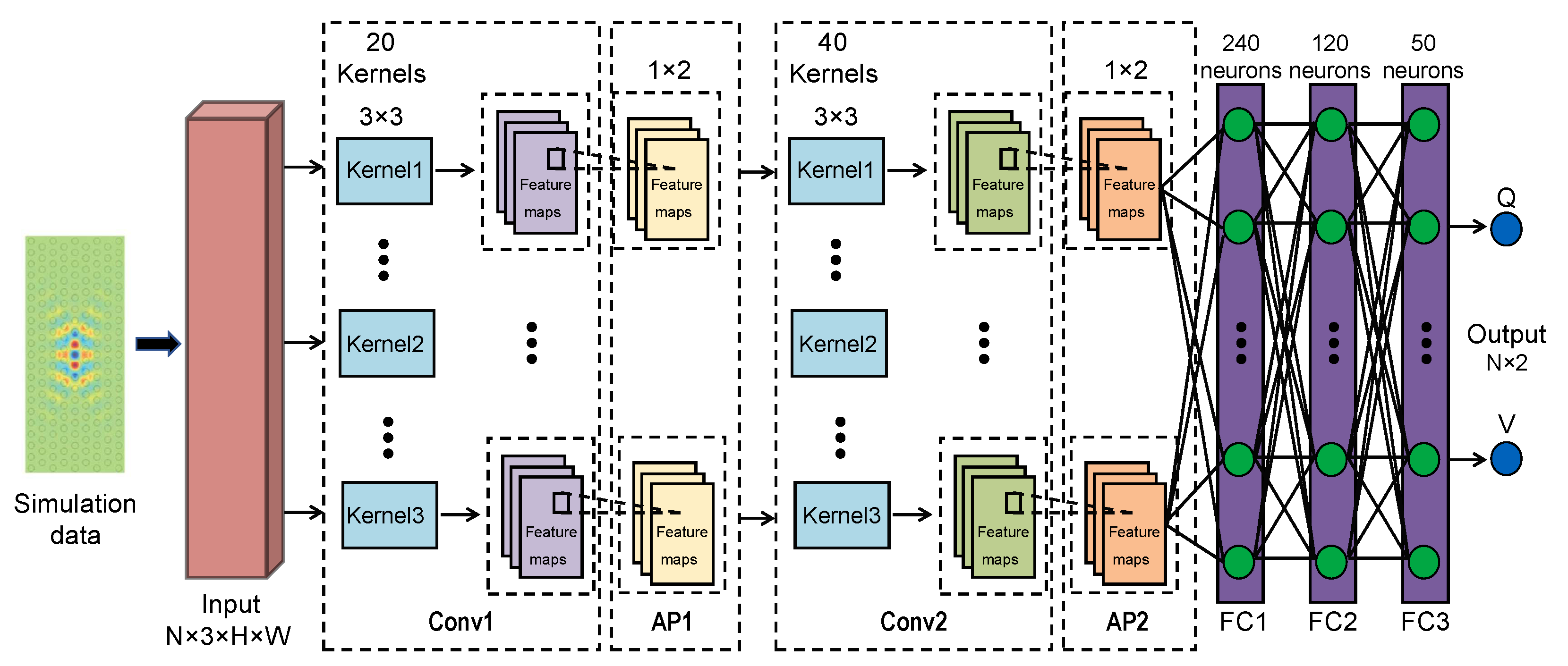
Figure 1. The DNN model (LRS-RCNN) to correlate the input (i.e., design parameters) with output (i.e., optical parameters such as Q and V) of nanophotonic structures. LRS-RCNN consists of two convolutional layers (Conv1 and Conv2), each accompanied by an averaging pooling (AP) operation, and lastly three FC layers. LRS-RCNN tackles the prediction of optical properties as a deep learning regression problem. The detailed specifications of the network and its hyperparameters are marked on the diagram and/or listed in Table 1.
Nanomaterials 12 01372 g001
Figure 2. Pictorial illustration of the working principle of convolutional neural networks (CNN) with average pooling. Moreover, the formula for calculating the output feature size of a convolutional operation is also shown.
Nanomaterials 12 01372 g002
Figure 3. LRS-RCNN algorithm for modeling nanophotonic structures, implemented with a multi-step process: choose the desired structure, randomly fluctuate its design parameters and compute the optical properties in FDTD (pre-training steps), preprocess the dataset (step 1), train the model (step 2), and finally validate the model (step 3). Not shown in the diagram are the adaptive learning rates and L2 regularization, which are both core components of this algorithm.
Nanomaterials 12 01372 g003
Figure 4. Nanobeam structure. (a) SEM image of an actual fabricated nanobeam by us. (b,c) The initial structure’s design parameters and optical properties, respectively. As shown, holes are elliptically shaped with r 1 and r 2 as its two axes. (d) A sample in the dataset with randomly shifted holes. Blue: original holes; red: shifted holes.
Nanomaterials 12 01372 g004
Figure 5. L3 nanocavity structure. (a) The initial structure’s design parameters and optical properties. Yellow box is the region where we randomly fluctuate the design parameters. Inset: the E y field of the initial structure. (b,c) Two samples in the dataset with randomly shifted holes. Black: original holes; red: shifted holes. Far right figures are magnified views of the configuration.
Nanomaterials 12 01372 g005
Figure 6. Learning curves of LRS-RCNN when trained to characterize nanobeam’s Q and V. Top panel contains results for Q: (a) prediction error ϵ p r e d vs. Epochs curve; (b) M S E vs. Epochs curve, for both training (yellow) and test (green) datasets. Min ϵ p r e d and M S E using the test dataset are also labeled on the figures, respectively. Bottom panel are the same results for V (c,d).
Nanomaterials 12 01372 g006
Figure 7. Validation results of the trained LRS-RCNN for nanobeam using the validation dataset. Plotted is the histogram of ϵ p r e d for Q in (a) and V in (b). The boxplot in (c) is extracted from data in (a), and (d) from (b). Inset data: minimum, average, and median ϵ p r e d values in the histograms.
Nanomaterials 12 01372 g007
Figure 8. Learning curves of LRS-RCNN when trained to characterize L3 nanocavity’s Q and V. Top panel contains results for Q: (a) prediction error ϵ p r e d vs. Epochs curve; (b) M S E vs. Epochs curve, for both training (yellow) and test (green) datasets. Min ϵ p r e d and M S E using the test dataset are also labeled on the figures, respectively. Bottom panel are the same results for V (c,d).
Nanomaterials 12 01372 g008
Figure 9. Validation results of the trained LRS-RCNN for L3 nanocavity using the validation dataset. Plotted is the histogram of ϵ p r e d for Q in (a) and V in (b). The boxplot in (c) is extracted from data in (a), and (d) from (b). Inset data: minimum, average, and median ϵ p r e d values in the histograms.
Nanomaterials 12 01372 g009
Figure 10. Results of training LRS-RCNN for L3 nanocavity when no LRS is used. The figure has the same order as Figure 8. One can observe the substantially noisier convergence curves in (ad) in this case compared to before.
Nanomaterials 12 01372 g010
Figure 11. Results of training LRS-RCNN for L3 when no L2 regularization is used. The figure has the same order as Figure 8. It is observed that large overfittings are present in (ad) in this case.
Nanomaterials 12 01372 g011
Table 1. Hyperparameters of LRS-RCNN.
HyperparameterValueHyperparameterValue
Conv120 3 × 3 kernels + 1 × 2 APFC1240 neurons
Conv240 3 × 3 kernels + 1 × 2 APFC2120 neurons
Paddings1FC350 neurons
Activation functionReLUNo. of Epochs700
Training batch size64Test batch size100
OptimizerSGDInitial learning rate0.01
Momentum0.5L2 regularization λ 0.001
Nanobeam’s ( H , W ) (1, 13)Learning rate schedulerReduceOnPlateau
L3’s ( H , W ) (5, 12)Loss function M S E
Table 2. Specifications of the dataset, generated according to Section 2.2, for training LRS-RCNN (DA = design parameter, OP = optical property, and DOF = degree of freedom). Left panel: nanobeam; right panel: L3 nanocavity. DAs such as “x locations” and “r” refer to the x coordinate and radius of each individual air hole, respectively. Corresponding OPs are computed by FDTD simulation.
Nanobeam DAsNanobeam OPsL3 DAsL3 OPs
r 1 Q-factorx locationsQ-factor
r 2 Modal volume Vy locationsModal volume V
x locations r
D O F = 13 × 3 = 39 D O F = 54 × 3 = 162
Publisher’s Note: MDPI stays neutral with regard to jurisdictional claims in published maps and institutional affiliations.