Appendix A. Invertible Autoencoder for Domain Adaptation
Figure A1.
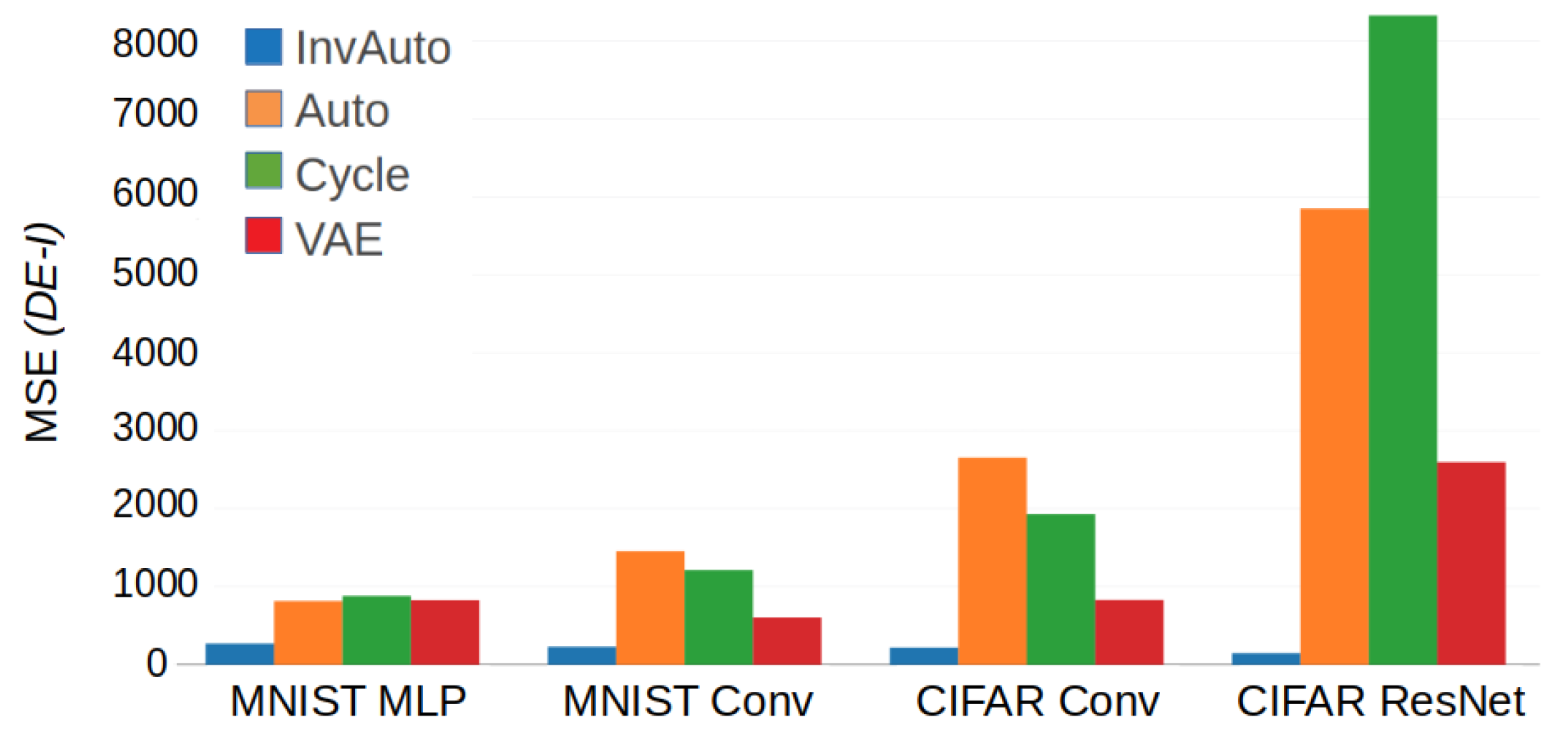
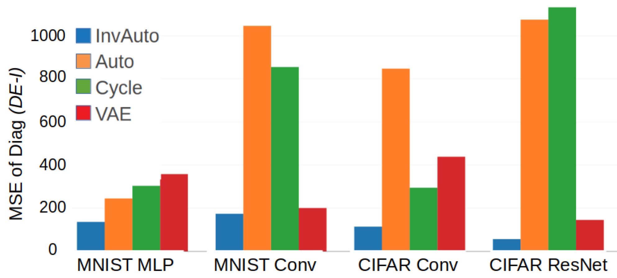
Comparison of the MSE of the diagonal of for InvAuto, Auto, Cycle, and VAE on MLP, convolutional (Conv), and ResNet architectures and MNIST and CIFAR datasets.
Figure A1.
Comparison of the MSE of the diagonal of for InvAuto, Auto, Cycle, and VAE on MLP, convolutional (Conv), and ResNet architectures and MNIST and CIFAR datasets.
Figure A2.
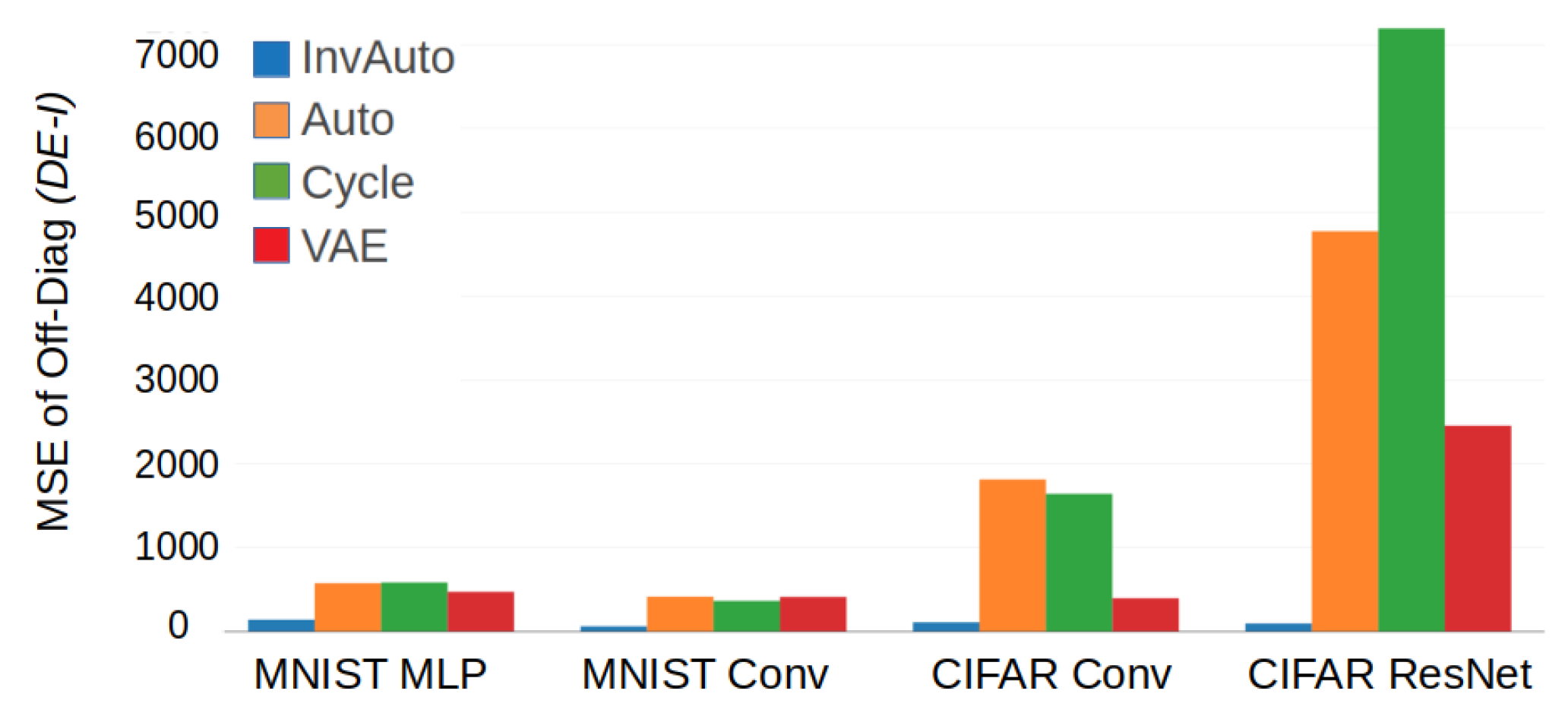
Comparison of the MSE of the off-diagonal of for InvAuto, Auto, Cycle, and VAE on MLP, convolutional (Conv), and ResNet architectures and MNIST and CIFAR dataset.
Figure A2.
Comparison of the MSE of the off-diagonal of for InvAuto, Auto, Cycle, and VAE on MLP, convolutional (Conv), and ResNet architectures and MNIST and CIFAR dataset.
Figure A3.
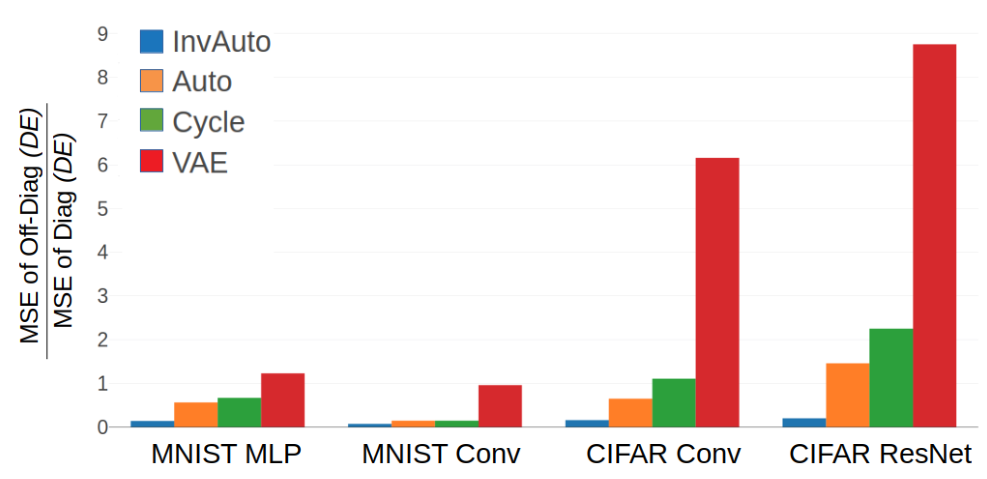
Comparison of the ratio of MSE of the off-diagonal and diagonal of for InvAuto, Auto, Cycle, and VAE on MLP, convolutional (Conv), and ResNet architectures and MNIST and CIFAR datasets.
Figure A3.
Comparison of the ratio of MSE of the off-diagonal and diagonal of for InvAuto, Auto, Cycle, and VAE on MLP, convolutional (Conv), and ResNet architectures and MNIST and CIFAR datasets.
Table A1.
Test reconstruction loss (MSE) for InvAuto, Auto, Cycle, and VAE on MLP, convolutional (Conv), and ResNet architectures and MNIST and CIFAR datasets. VAE has significantly higher reconstruction loss by construction.
Table A1.
Test reconstruction loss (MSE) for InvAuto, Auto, Cycle, and VAE on MLP, convolutional (Conv), and ResNet architectures and MNIST and CIFAR datasets. VAE has significantly higher reconstruction loss by construction.
| Dataset and Model | InvAuto | Auto | Cycle | VAE |
|---|
| MNIST MLP | | | | |
| MNIST Conv | | | | |
| CIFAR Conv | | | | |
| CIFAR ResNet | | | | |
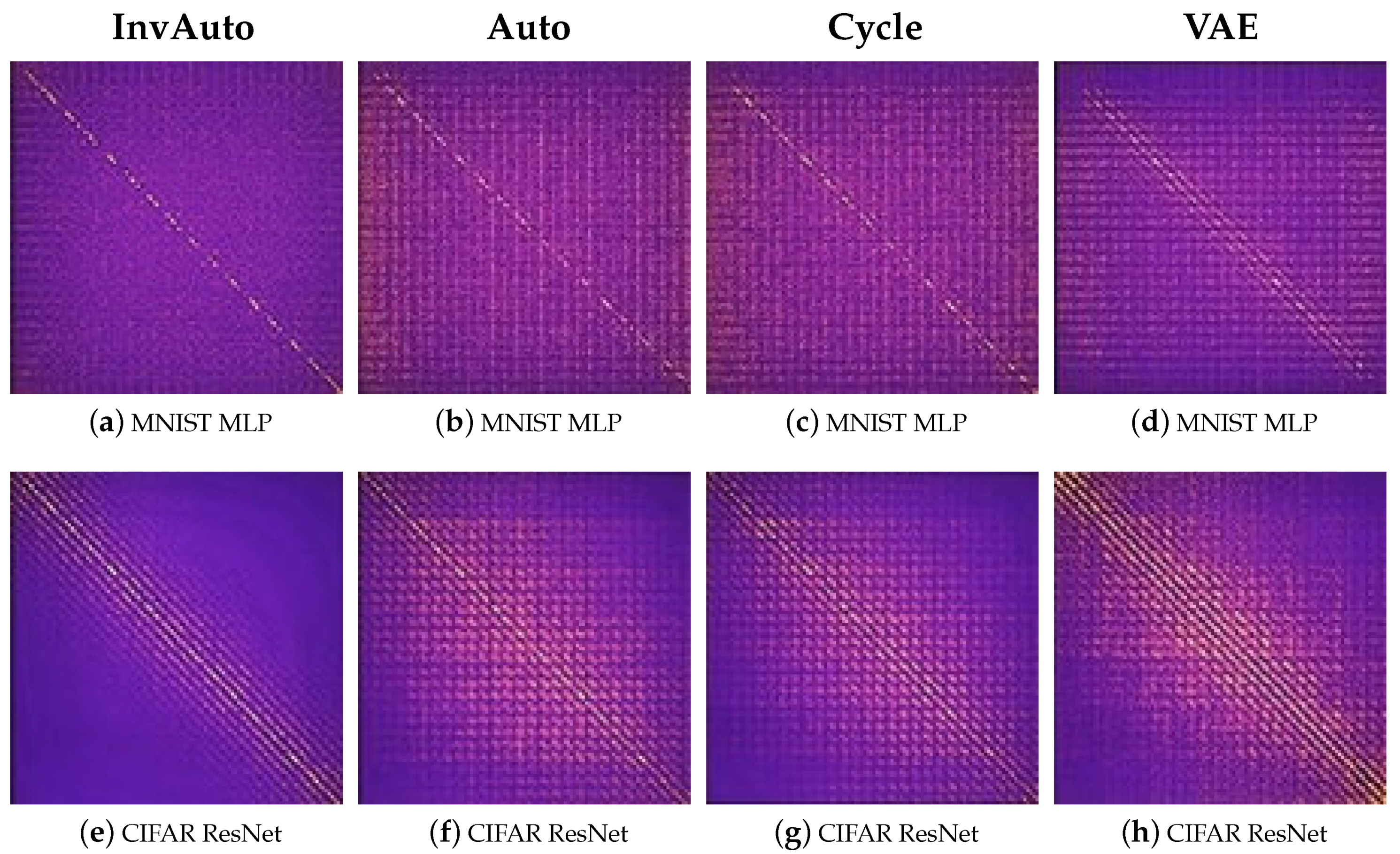
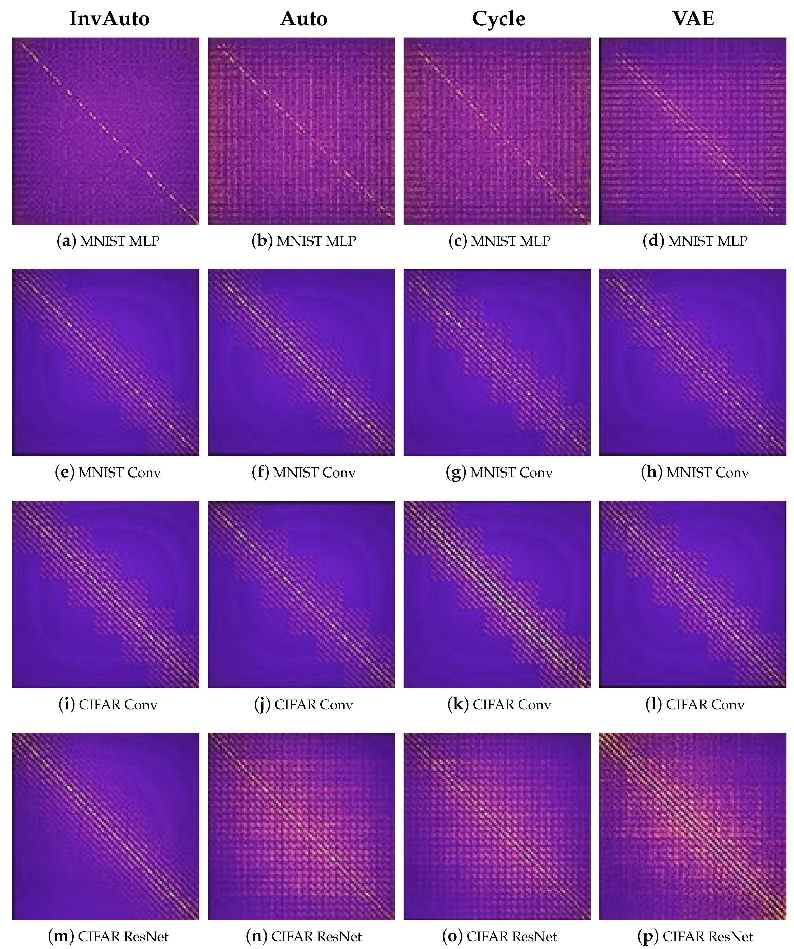
Figure A4.
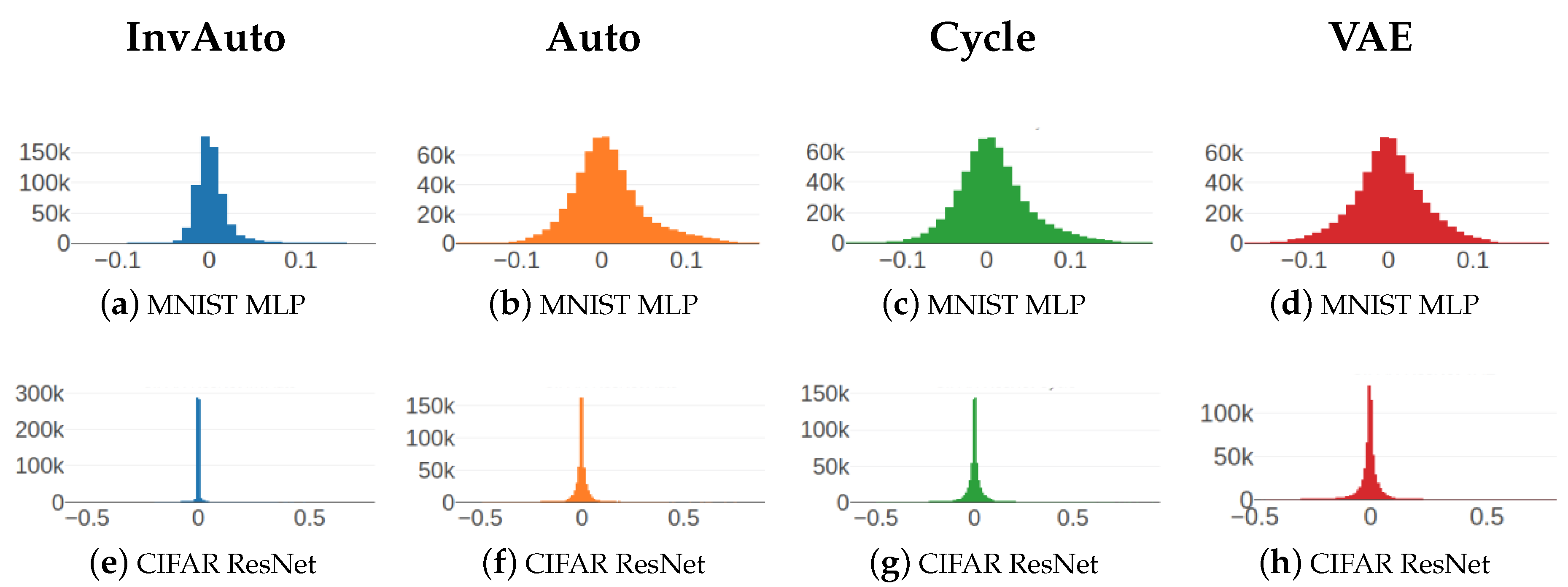
Heatmap of the values of matrix for InvAuto, (a,e,i,m) Auto (b,f,j,n), Cycle (c,g,k,o), and VAE (d,h,l,p) on MLP, convolutional (Conv), and ResNet architectures and MNIST and CIFAR datasets. Matrices E and D are constructed by multiplying the weight matrices of consecutive layers of encoder and decoder, respectively. In case of InvAuto, is the closest to the identity matrix.
Figure A4.
Heatmap of the values of matrix for InvAuto, (a,e,i,m) Auto (b,f,j,n), Cycle (c,g,k,o), and VAE (d,h,l,p) on MLP, convolutional (Conv), and ResNet architectures and MNIST and CIFAR datasets. Matrices E and D are constructed by multiplying the weight matrices of consecutive layers of encoder and decoder, respectively. In case of InvAuto, is the closest to the identity matrix.
Additional Experimental Results for
Section 5
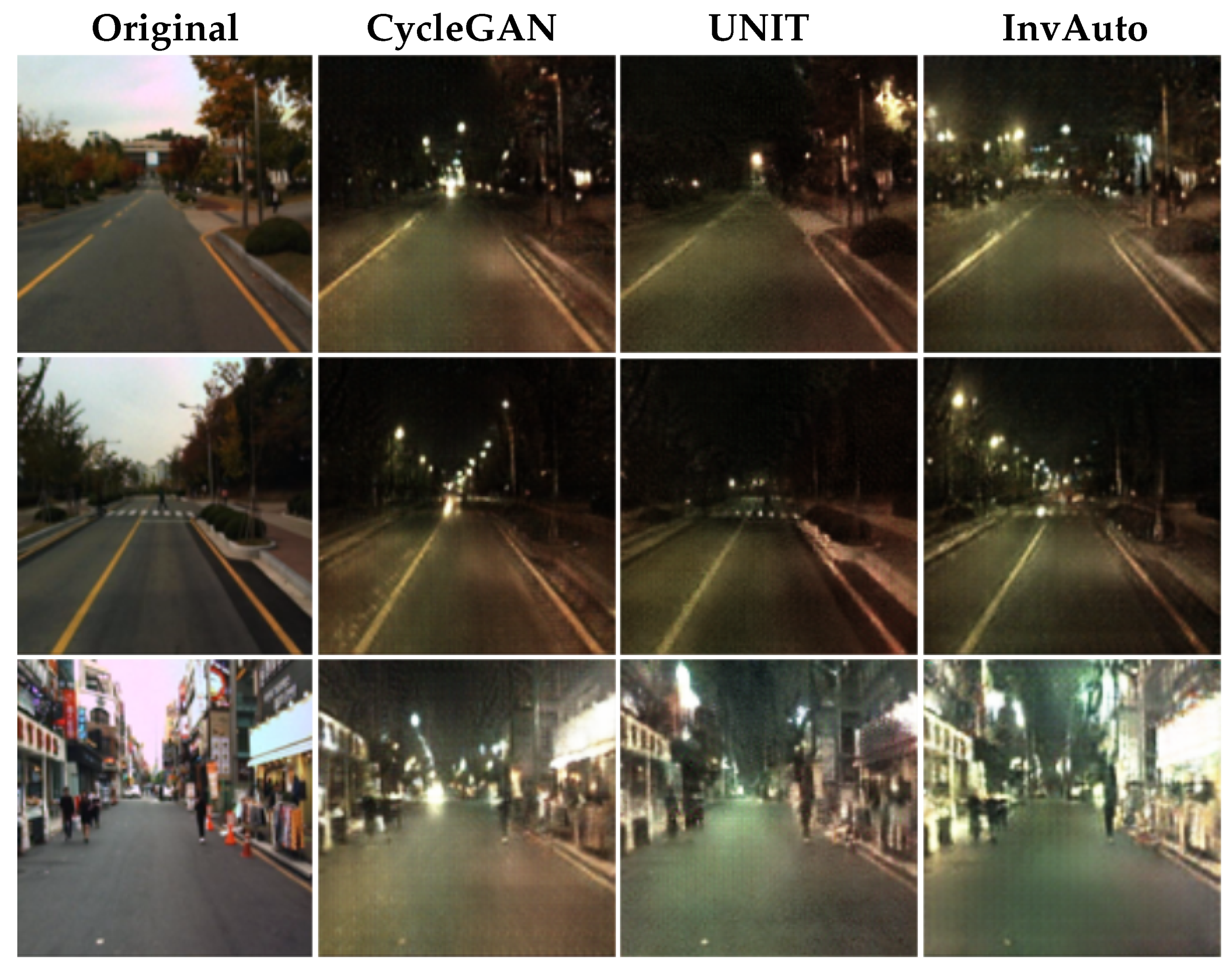
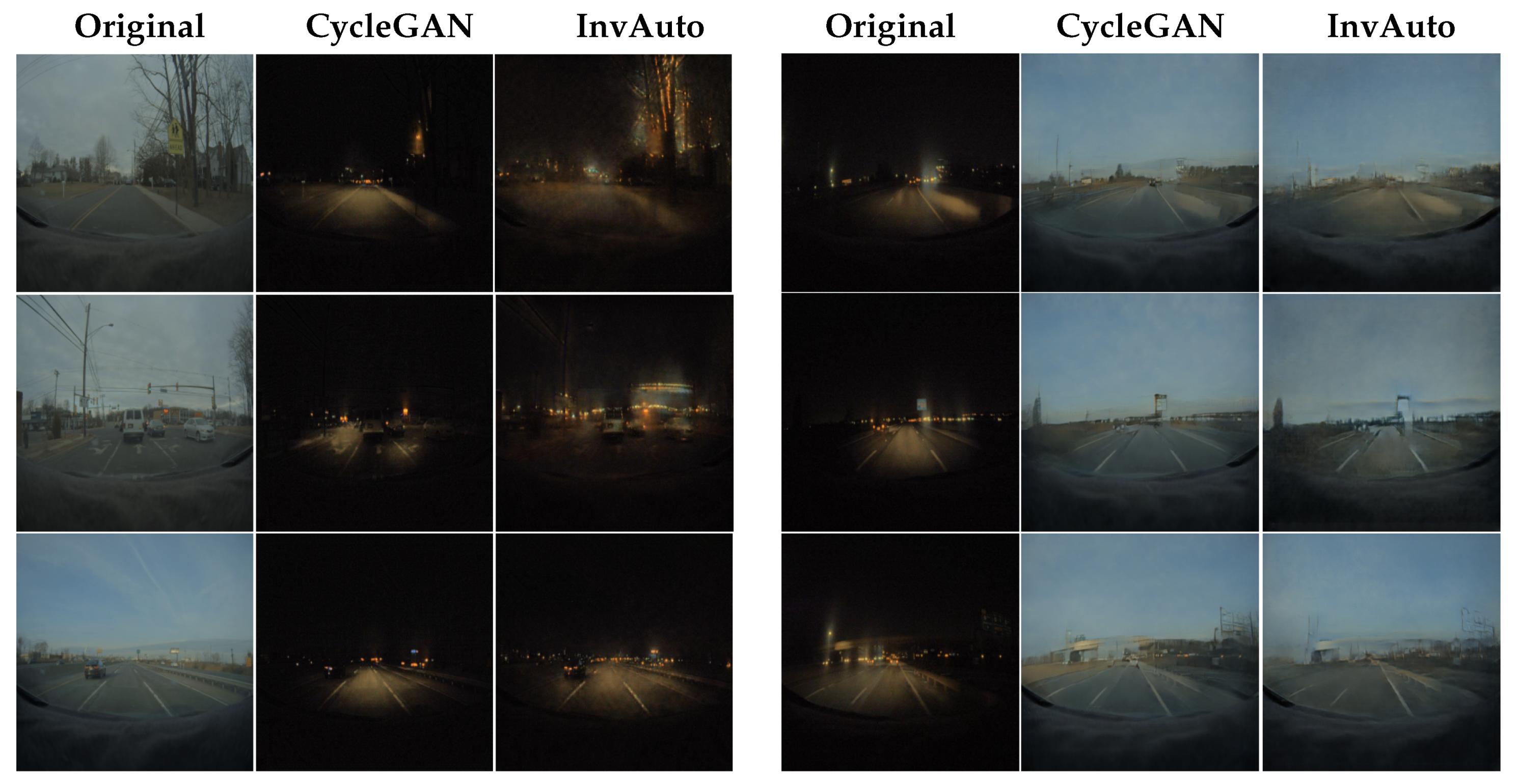
Figure A5.
Day-to-night image conversion.
Figure A5.
Day-to-night image conversion.
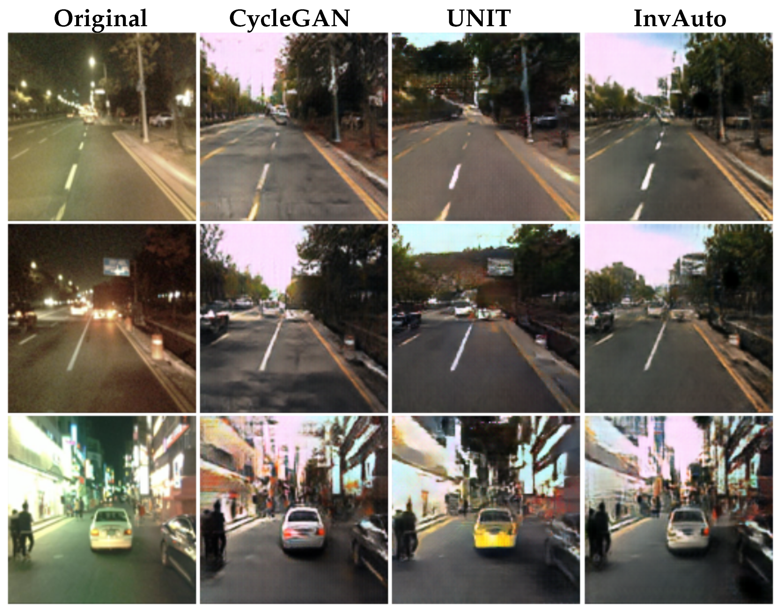
Figure A6.
Night-to-day image conversion.
Figure A6.
Night-to-day image conversion.
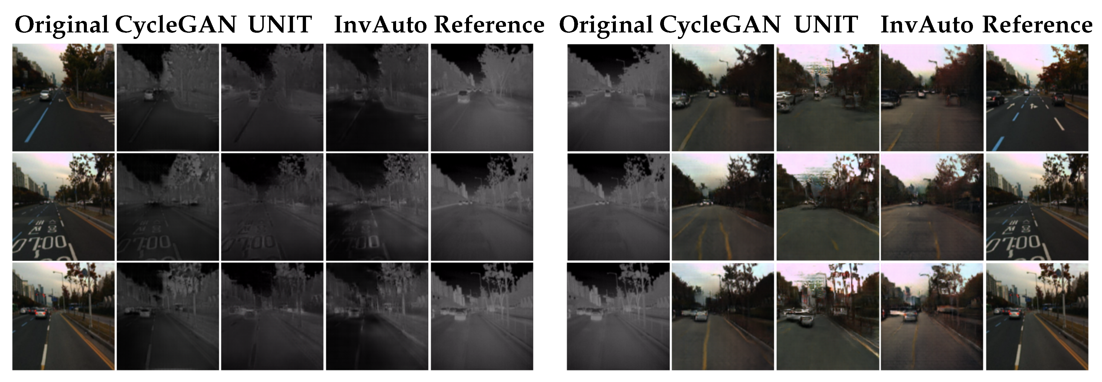
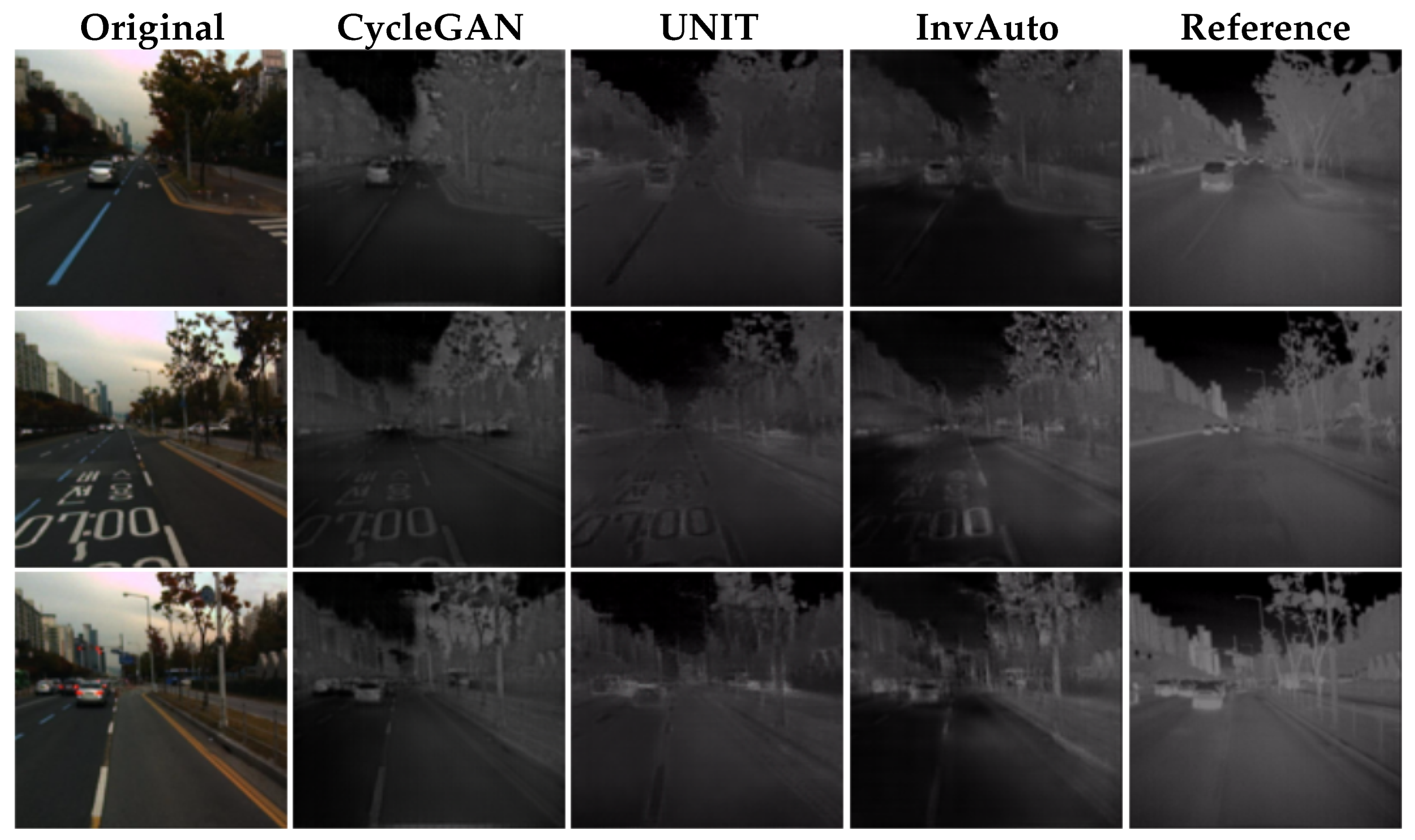
Figure A7.
Day-to-thermal image conversion.
Figure A7.
Day-to-thermal image conversion.
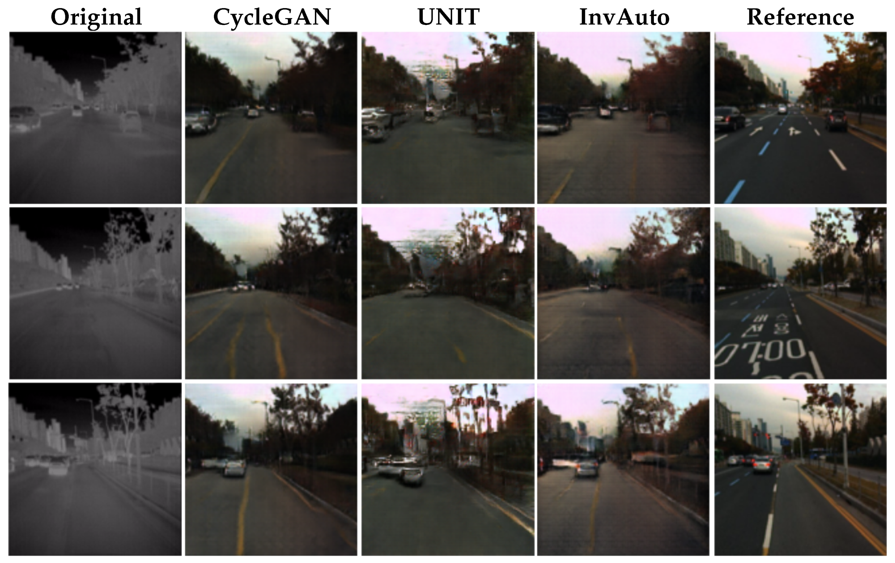
Figure A8.
Thermal-to-day image conversion.
Figure A8.
Thermal-to-day image conversion.
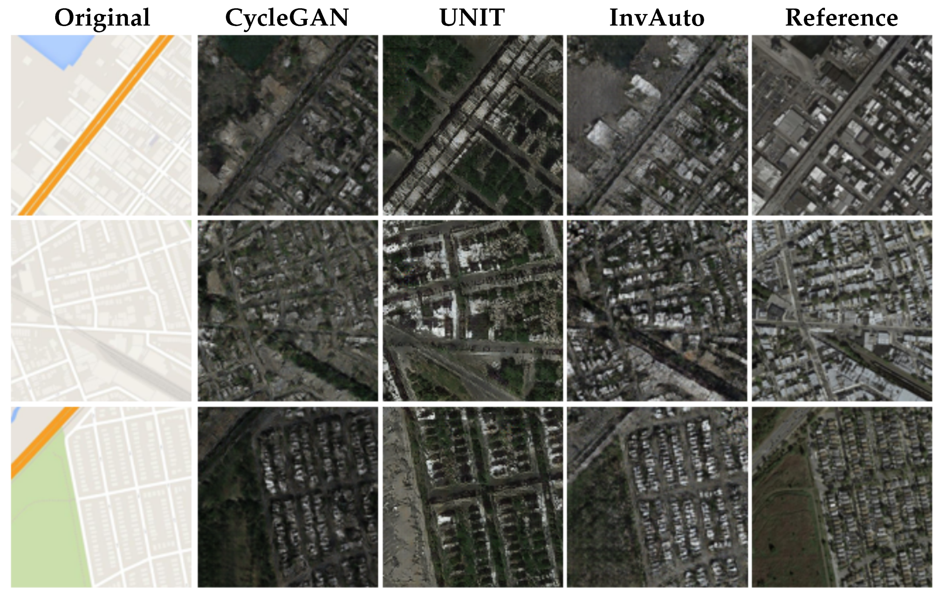
Figure A9.
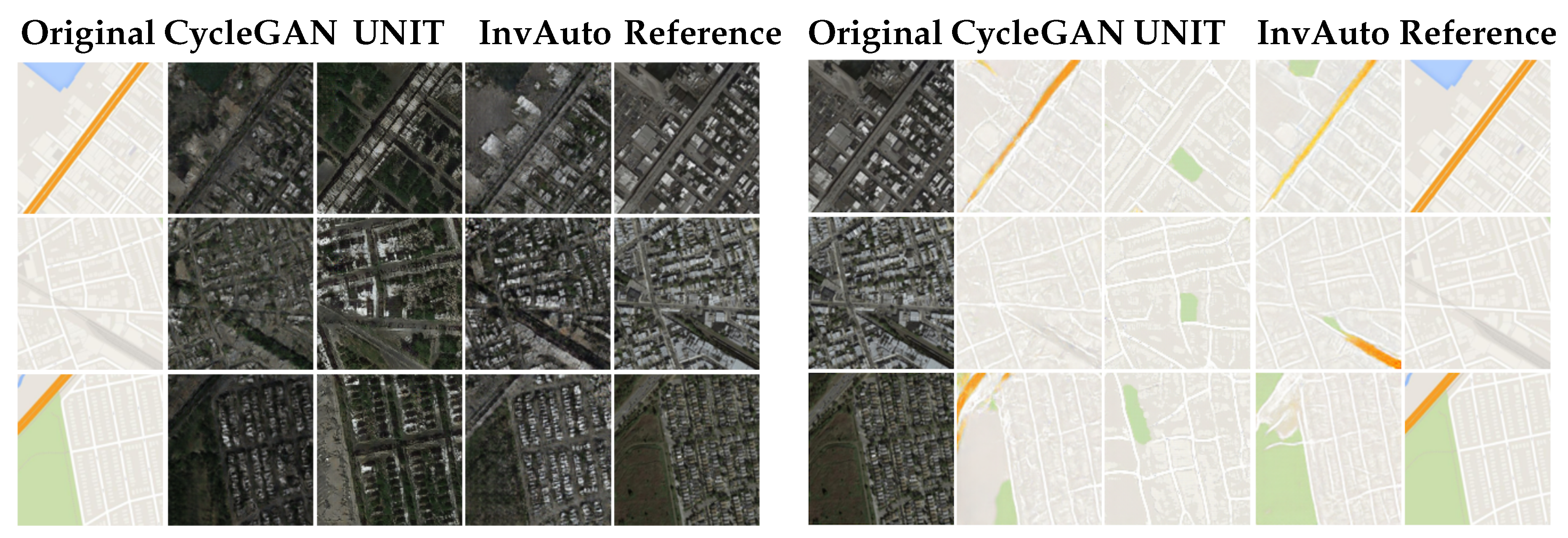
Maps-to-satellite image conversion.
Figure A9.
Maps-to-satellite image conversion.
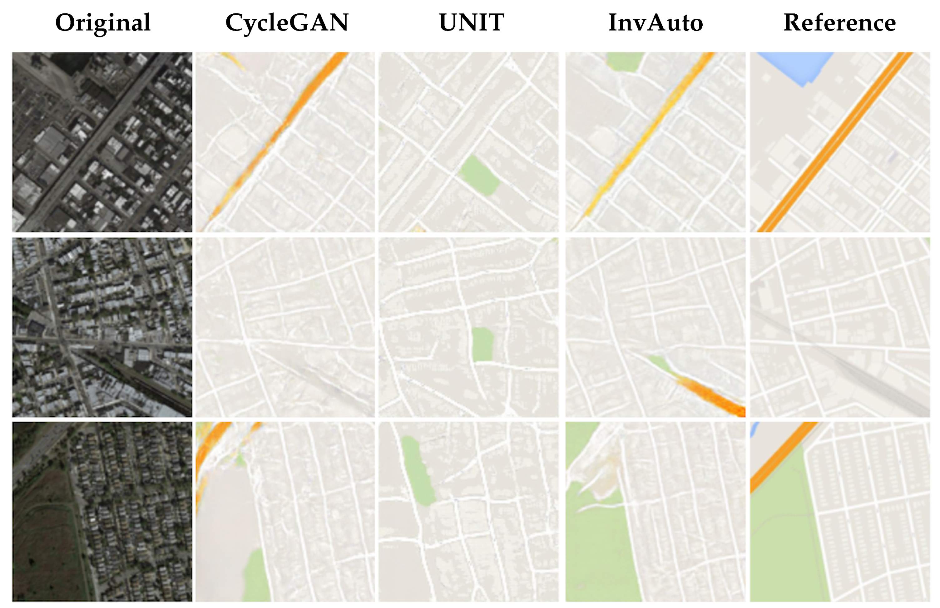
Figure A10.
Satellite-to-maps image conversion.
Figure A10.
Satellite-to-maps image conversion.
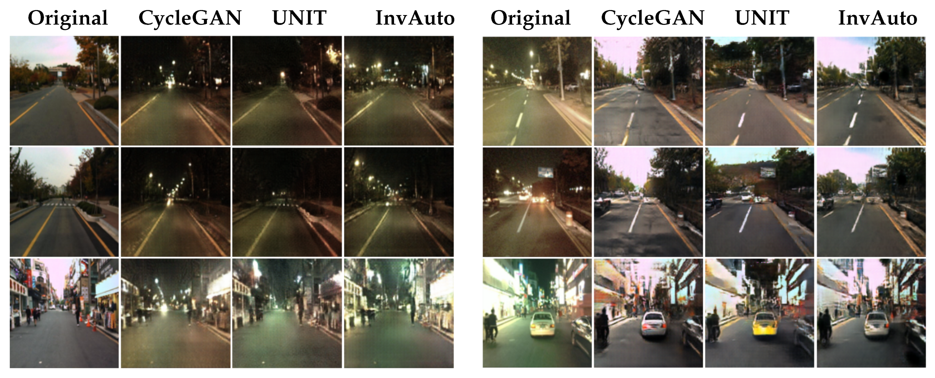
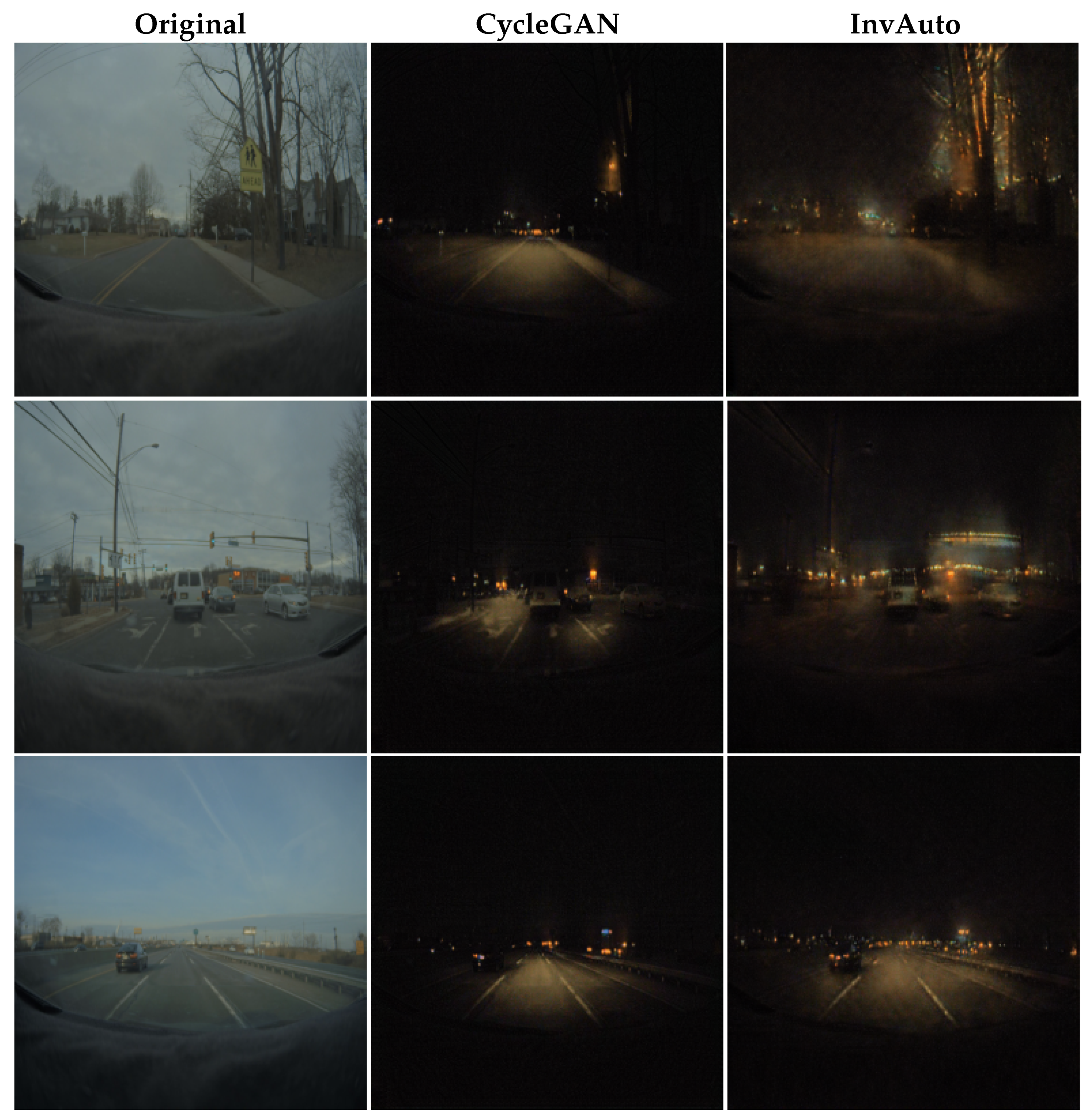
Figure A11.
Experimental results with autonomous driving system: day-to-night conversion.
Figure A11.
Experimental results with autonomous driving system: day-to-night conversion.
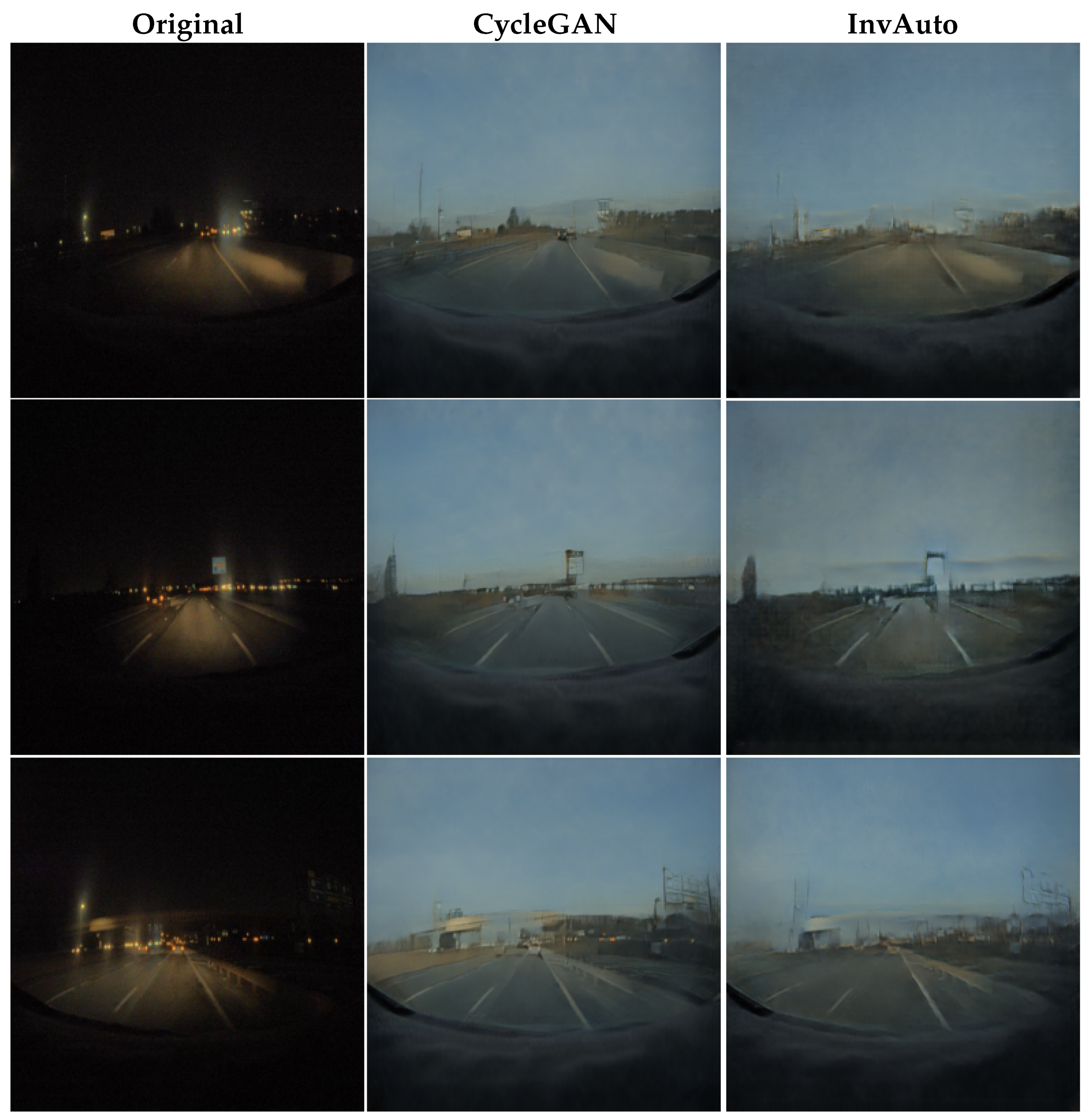
Figure A12.
Experimental results with autonomous driving system: night-to-day conversion.
Figure A12.
Experimental results with autonomous driving system: night-to-day conversion.
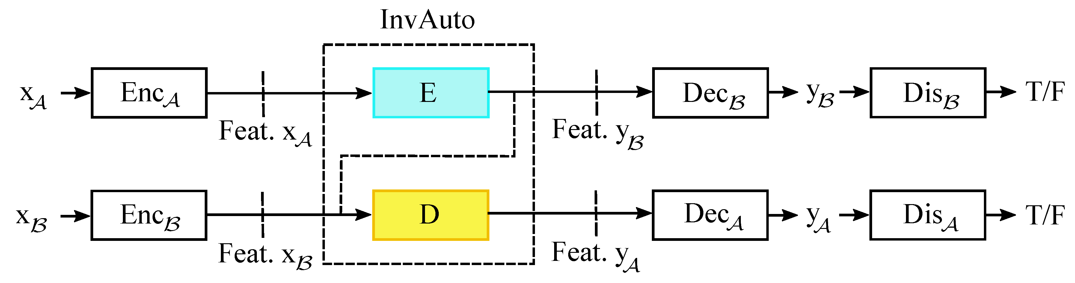
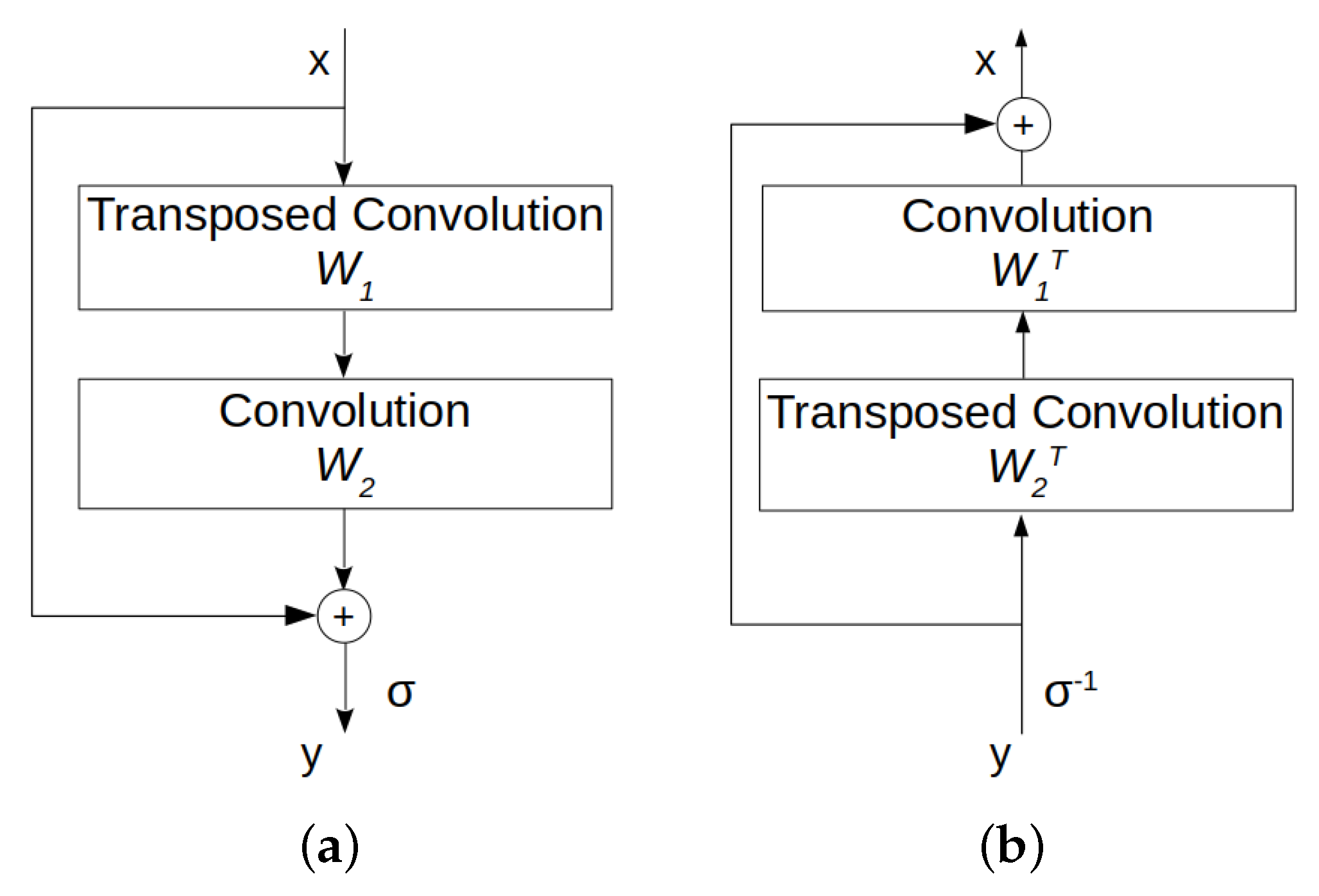
Generator architecture Our implementation of InvAuto contains 18 invertible residual blocks for both
and
images, where 9 blocks are used in the encoder and the remaining in the decoder. All layers in the decoder are the inverted versions of encoder’s layers. We furthermore add two down-sampling layers and two up-sampling layers for the model trained on
images, and three down-sampling layers and three up-sampling layers for the model trained on
images. The details of the generator’s architecture are listed in
Table A3 and
Table A4. For convenience, we use Conv to denote convolutional layer, ConvNormReLU to denote Convolutional-InstanceNorm-LeakyReLU layer, InvRes to denote invertible residual block, and Tanh to denote hyperbolic tangent activation function. The negative slope of LeakyReLU function is set to
. All filters are square and we have the following notations:
K represents filter size and
F represents the number of output feature maps. The paddings are added correspondingly.
Discriminator architecture We use similar discriminator architecture as PatchGAN [
1]. It is described in
Table A2. We use this architecture for training both on
and
images.
Criterion and Optimization At training, we set
and use
loss for the cycle consistency in Equation (
12). We use Adam optimizer [
32] with learning rate
= 0.0002,
and
. We also add
penalty with weight
.
Table A2.
Discriminator for both 128 × 128 and 512 × 512 images.
Table A2.
Discriminator for both 128 × 128 and 512 × 512 images.
| Name | Stride | Filter |
|---|
| ConvNormReLU | 2 × 2 | K4-F64 |
| ConvNormReLU | 2 × 2 | K4-F128 |
| ConvNormReLU | 2 × 2 | K4-F256 |
| ConvNormReLU | 1 × 1 | K4-F512 |
| Conv | 1 × 1 | K4-F1 |
Table A3.
Generator for 128 × 128 images.
Table A3.
Generator for 128 × 128 images.
| Name | Stride | Filter |
|---|
| ConvNormReLU | 1 × 1 | K7-F64 |
| ConvNormReLU | 2 × 2 | K3-F128 |
| ConvNormReLU | 2 × 2 | K3-F256 |
| InvRes | 1 × 1 | K3-F256 |
| InvRes | 1 × 1 | K3-F256 |
| InvRes | 1 × 1 | K3-F256 |
| InvRes | 1 × 1 | K3-F256 |
| InvRes | 1 × 1 | K3-F256 |
| InvRes | 1 × 1 | K3-F256 |
| InvRes | 1 × 1 | K3-F256 |
| InvRes | 1 × 1 | K3-F256 |
| InvRes | 1 × 1 | K3-F256 |
| ConvNormReLU | 1/2 × 1/2 | K3-F128 |
| ConvNormReLU | 1/2 × 1/2 | K3-F64 |
| Conv | 1 × 1 | K7-F3 |
| Tanh | | |
Table A4.
Generator for 512 × 512 images.
Table A4.
Generator for 512 × 512 images.
| Name | Stride | Filter |
|---|
| ConvNormReLU | 1 × 1 | K7-F64 |
| ConvNormReLU | 2 × 2 | K3-F128 |
| ConvNormReLU | 2 × 2 | K3-F256 |
| ConvNormReLU | 2 × 2 | K3-F512 |
| InvRes | 1 × 1 | K3-F512 |
| InvRes | 1 × 1 | K3-F512 |
| InvRes | 1 × 1 | K3-F512 |
| InvRes | 1 × 1 | K3-F512 |
| InvRes | 1 × 1 | K3-F512 |
| InvRes | 1 × 1 | K3-F512 |
| InvRes | 1 × 1 | K3-F512 |
| InvRes | 1 × 1 | K3-F512 |
| InvRes | 1 × 1 | K3-F512 |
| ConvNormReLU | 1/2 × 1/2 | K3-F256 |
| ConvNormReLU | 1/2 × 1/2 | K3-F128 |
| ConvNormReLU | 1/2 × 1/2 | K3-F64 |
| Conv | 1 × 1 | K7-F3 |
| Tanh | | |


