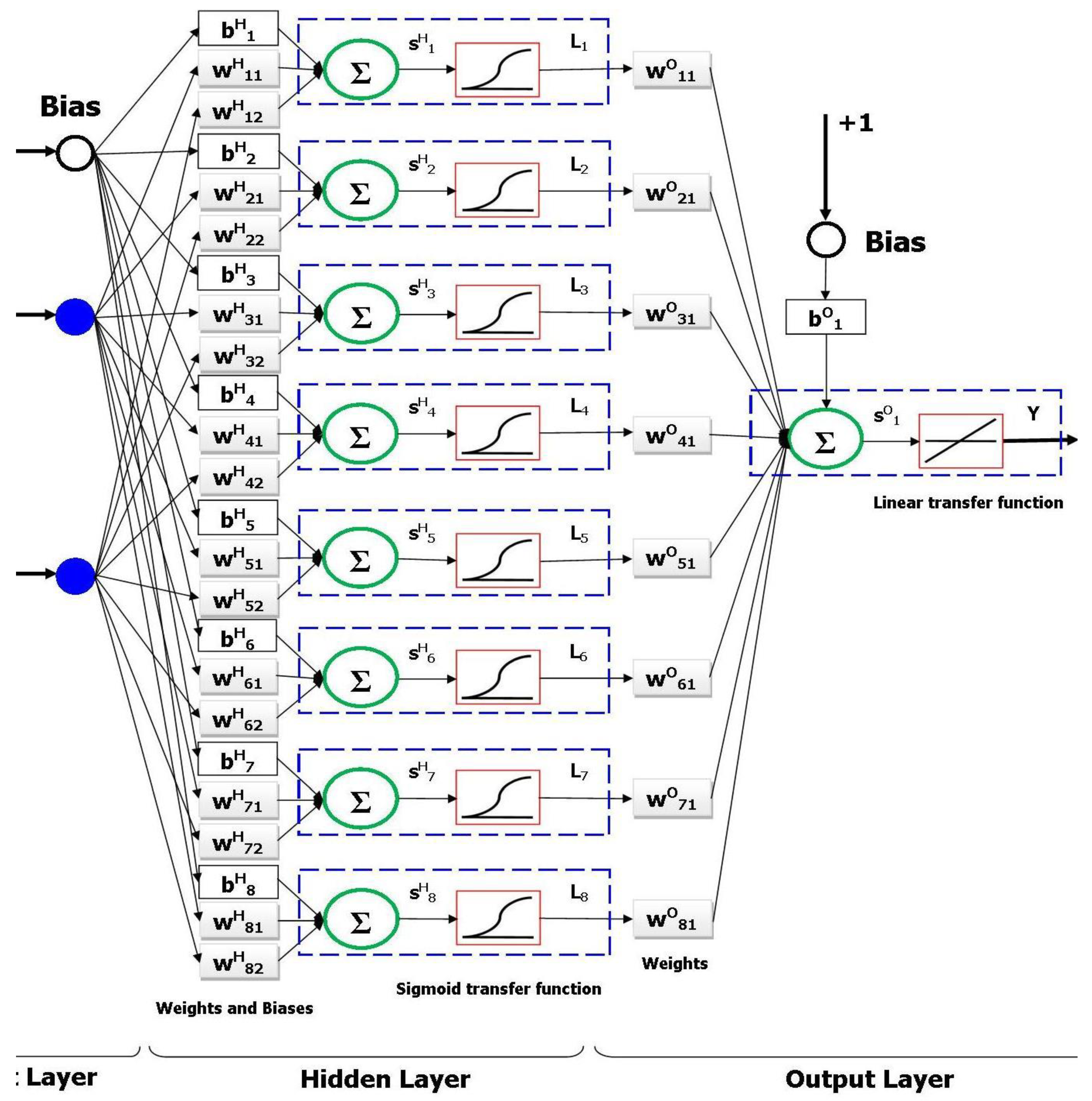
Figure 1.
Structure of the proposed three layers feed-forward neural network model.
Figure 1.
Structure of the proposed three layers feed-forward neural network model.
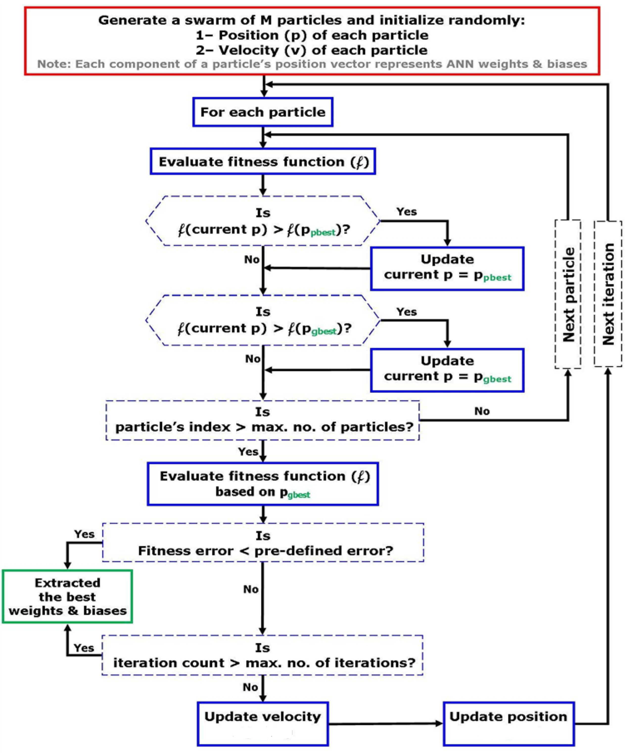
Figure 2.
Flowchart of the Particle Swarm Optimization (PSO)-based optimization algorithm for evolving the weights and biases of the constructed artificial neural networks (ANN).
Figure 2.
Flowchart of the Particle Swarm Optimization (PSO)-based optimization algorithm for evolving the weights and biases of the constructed artificial neural networks (ANN).
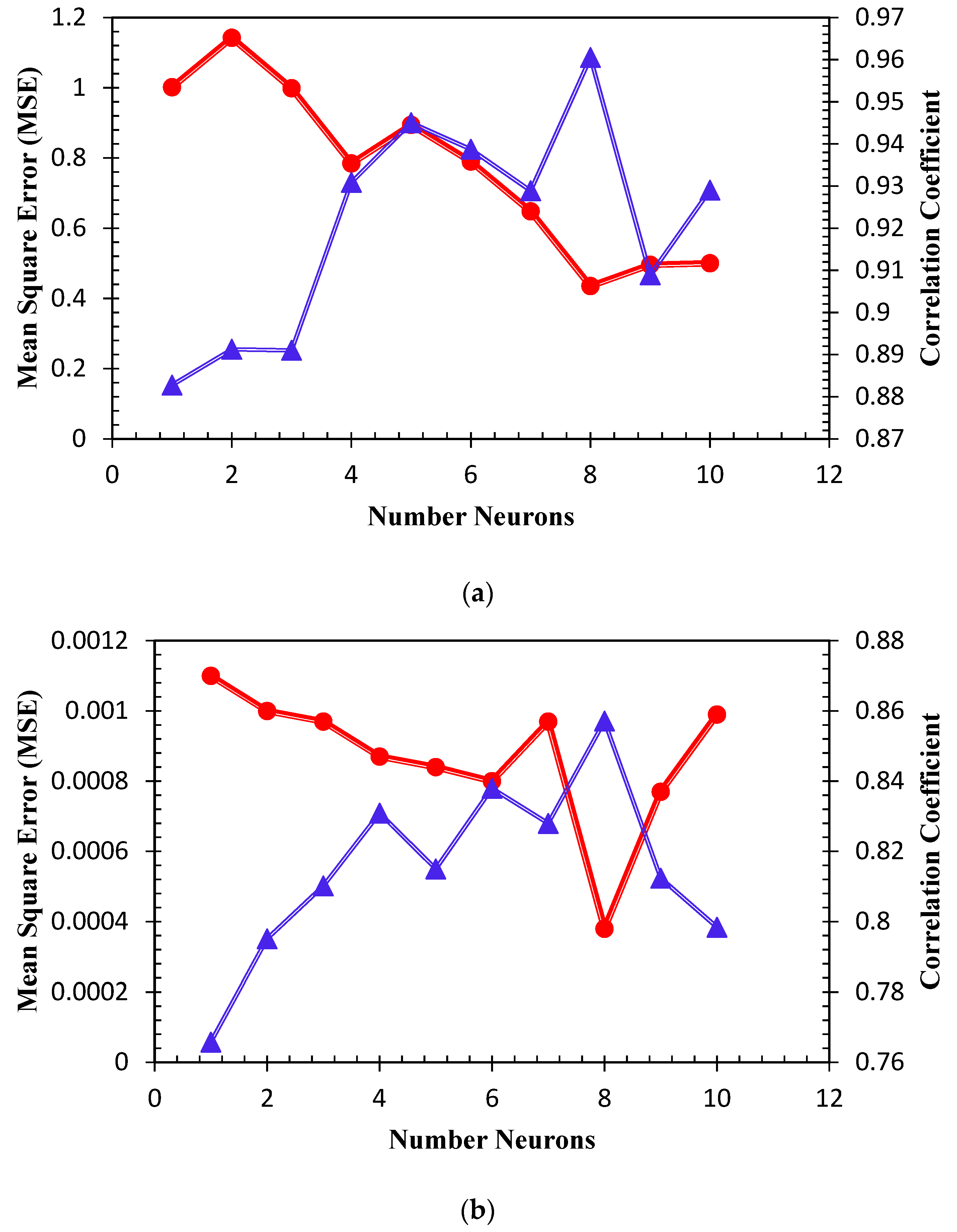
Figure 3.
Effect of the number of hidden neurons on the performance of the PSO-ANN model in terms of R2 and MSE values for (a) viscosity (b) thermal conductivity.
Figure 3.
Effect of the number of hidden neurons on the performance of the PSO-ANN model in terms of R2 and MSE values for (a) viscosity (b) thermal conductivity.
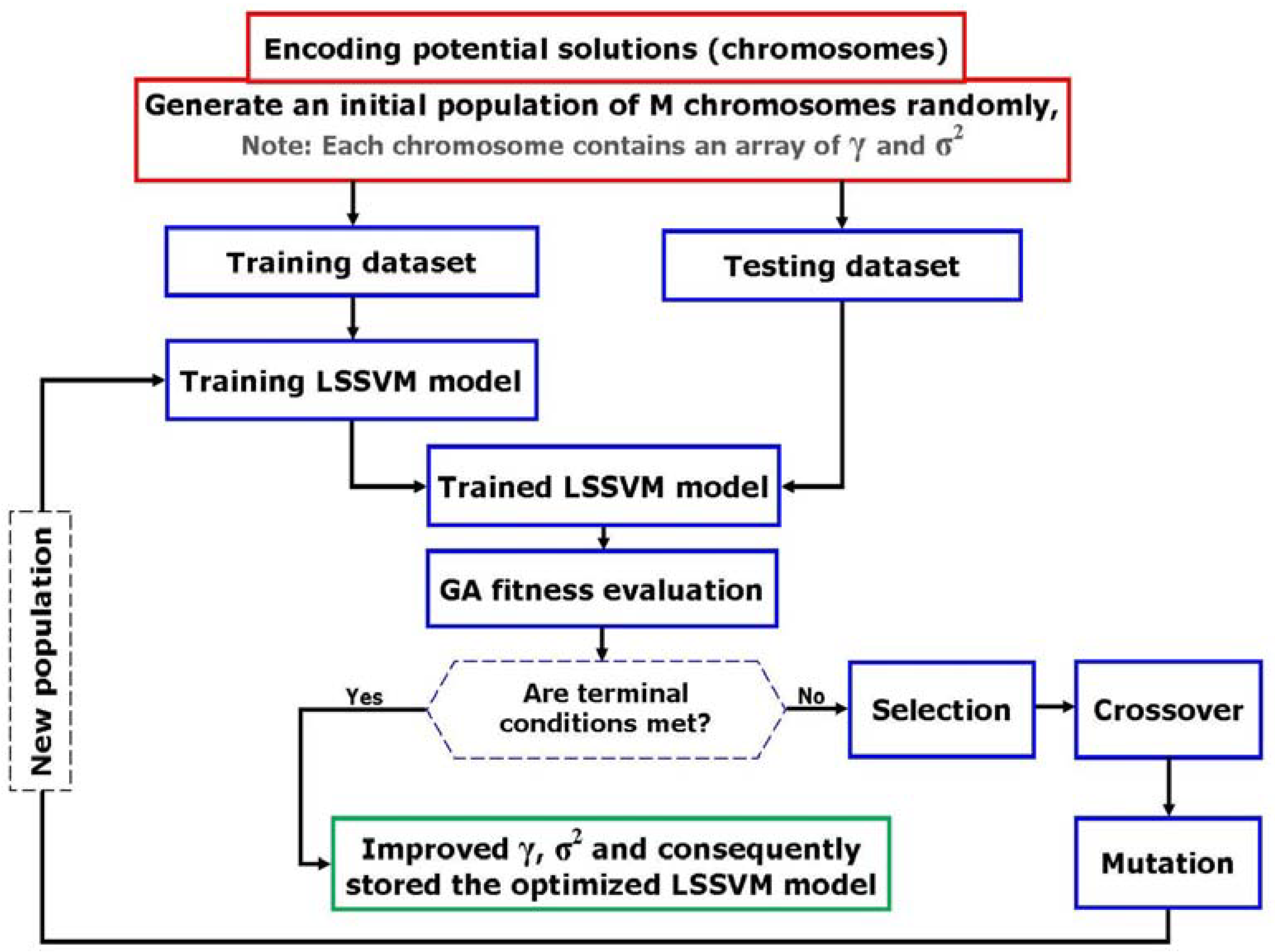
Figure 4.
Flowchart of GA-based optimization algorithm to adjust the embedded parameters of LSSVM model.
Figure 4.
Flowchart of GA-based optimization algorithm to adjust the embedded parameters of LSSVM model.
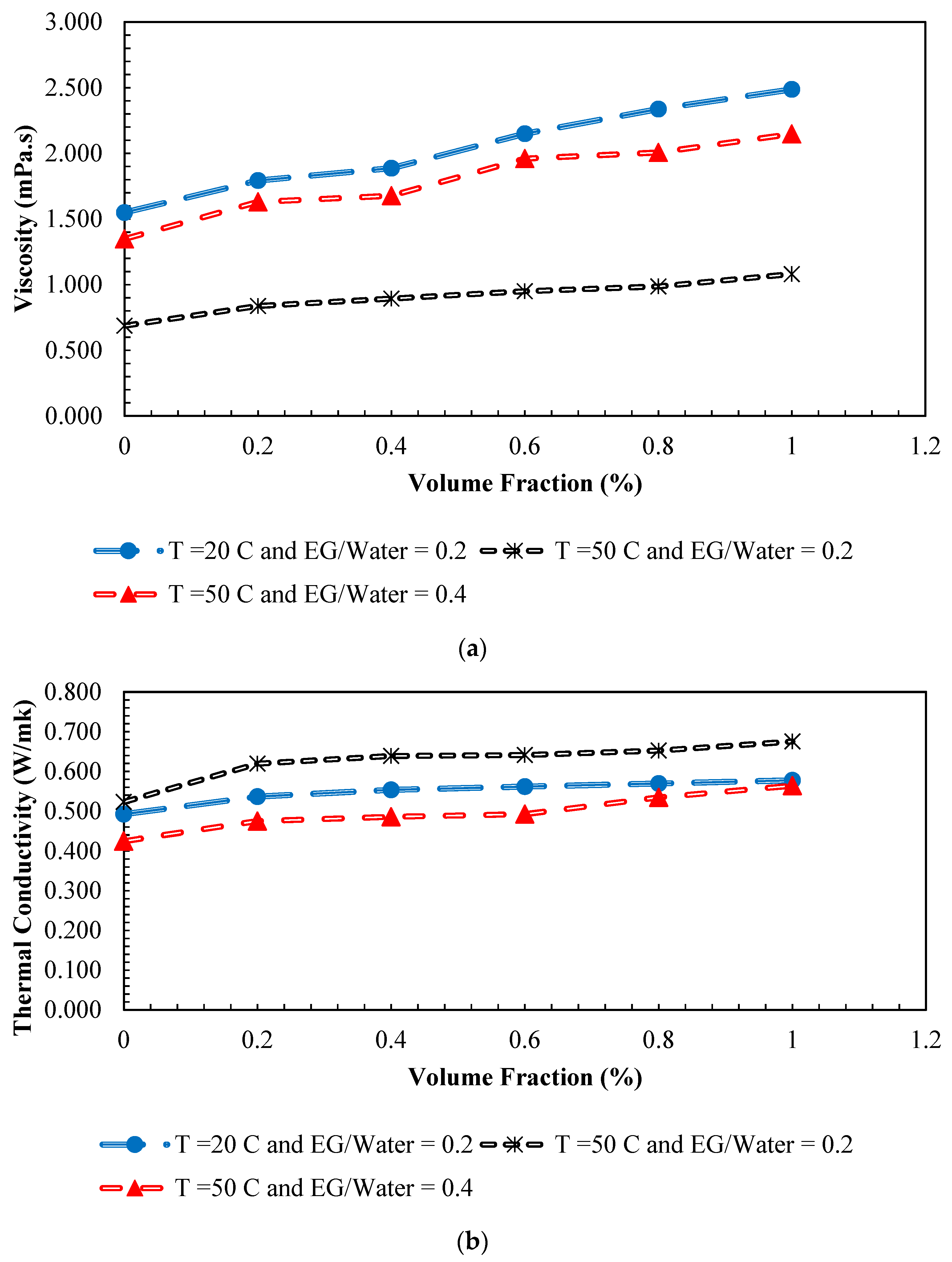
Figure 5.
Variation of viscosity (a) and thermal conductivity (b) versus volume fraction at different temperatures.
Figure 5.
Variation of viscosity (a) and thermal conductivity (b) versus volume fraction at different temperatures.
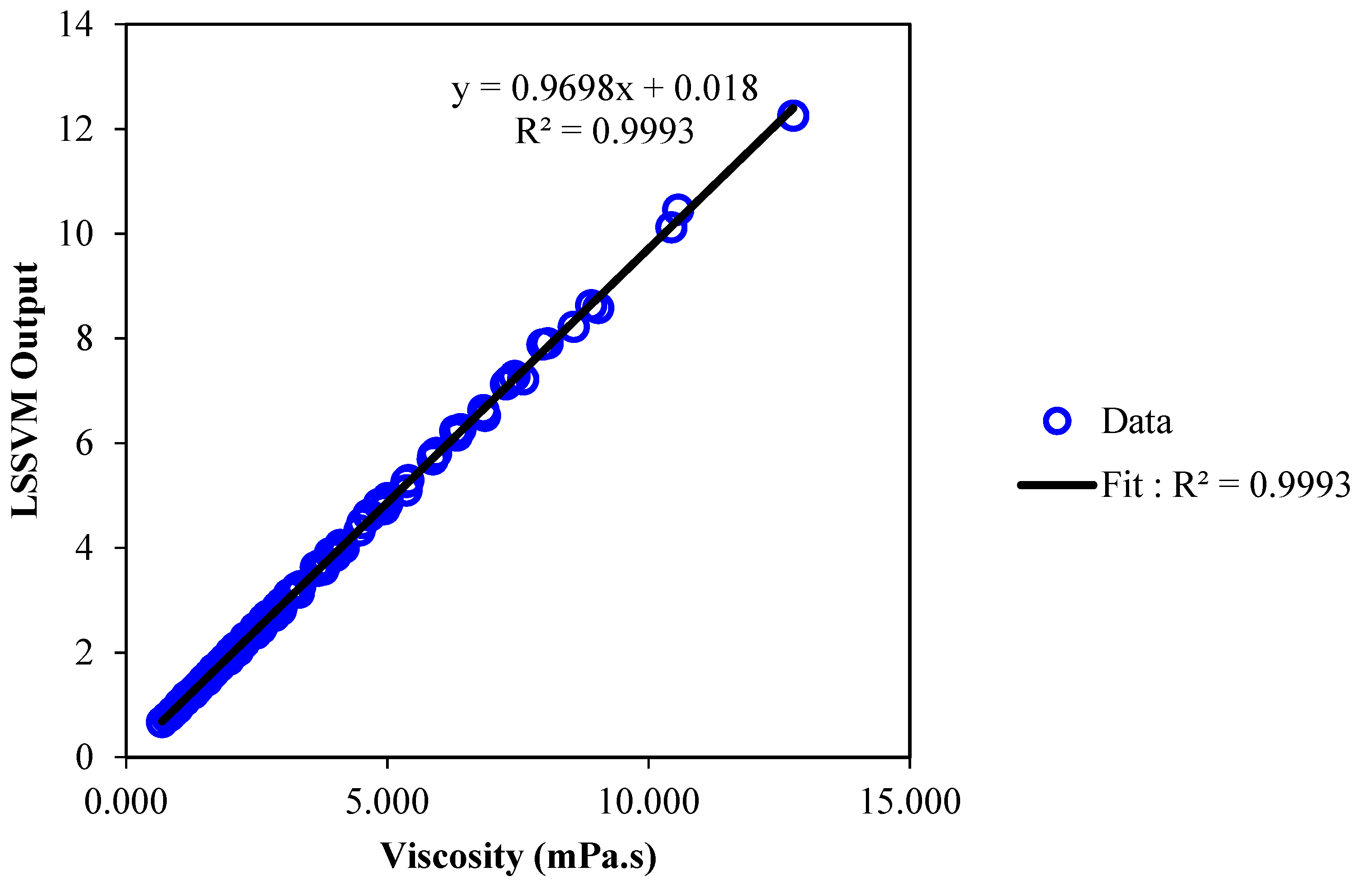
Figure 6.
Regression plot of the proposed vector machine model versus actual viscosity of /ethlyene glycol-water nanofluid.
Figure 6.
Regression plot of the proposed vector machine model versus actual viscosity of /ethlyene glycol-water nanofluid.
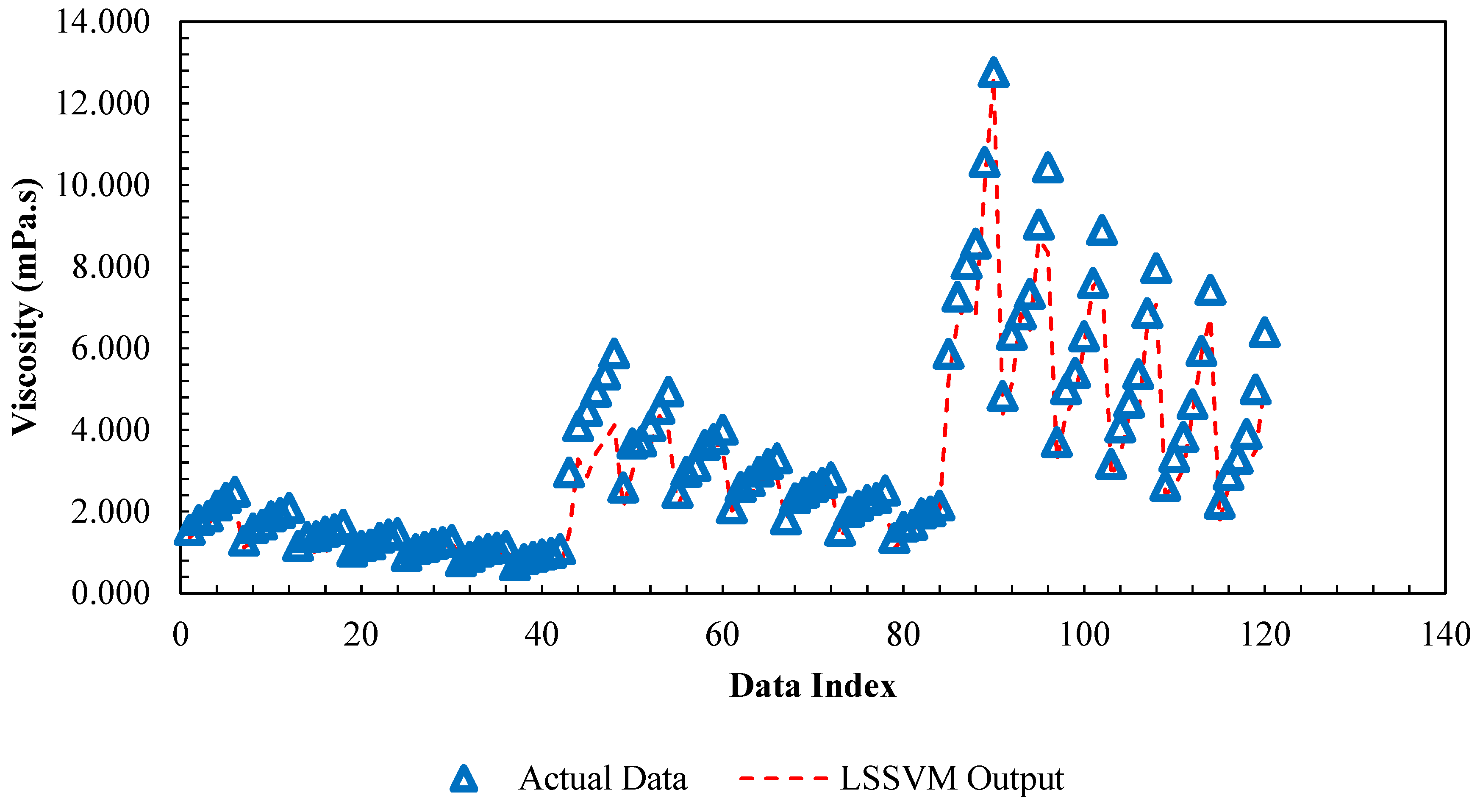
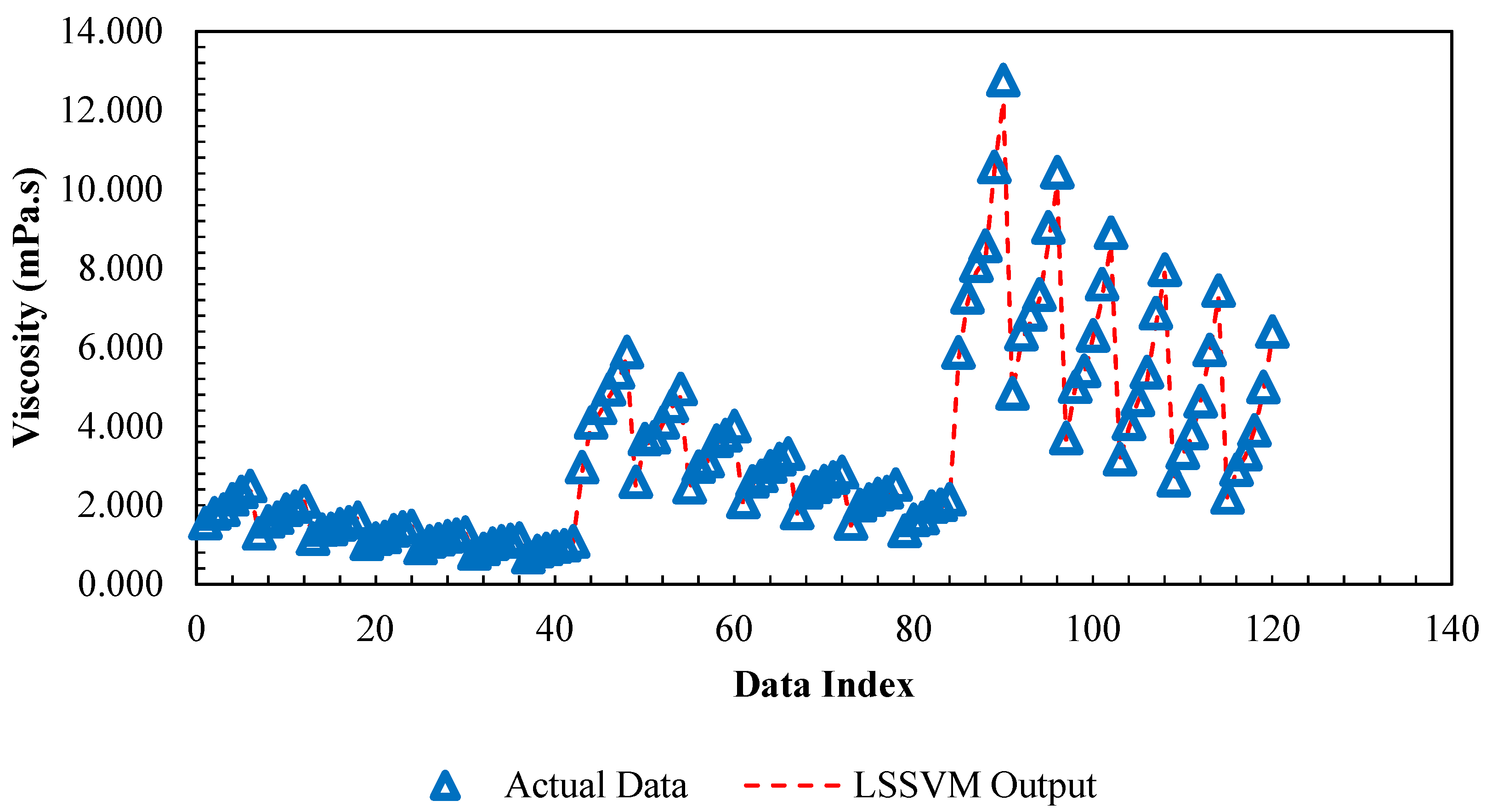
Figure 7.
Comparison between actual viscosity of /ethylene glycol-water nanofluid and predicted values by Least Square Support Vector Machine (LSSVM) model versus relevant data index.
Figure 7.
Comparison between actual viscosity of /ethylene glycol-water nanofluid and predicted values by Least Square Support Vector Machine (LSSVM) model versus relevant data index.
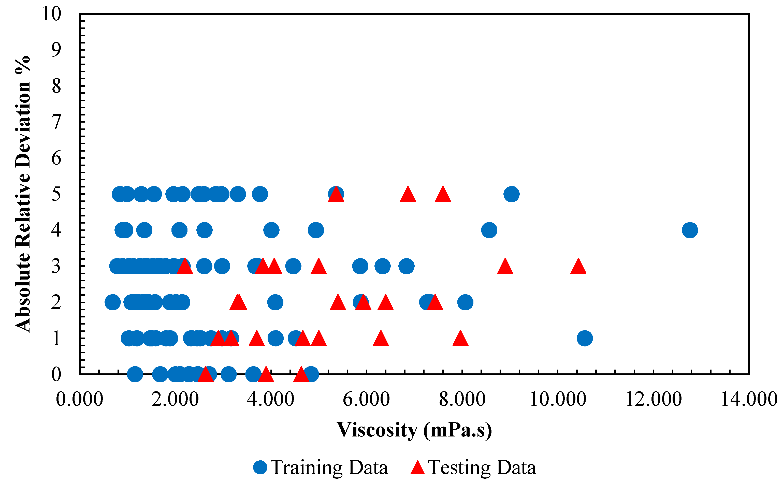
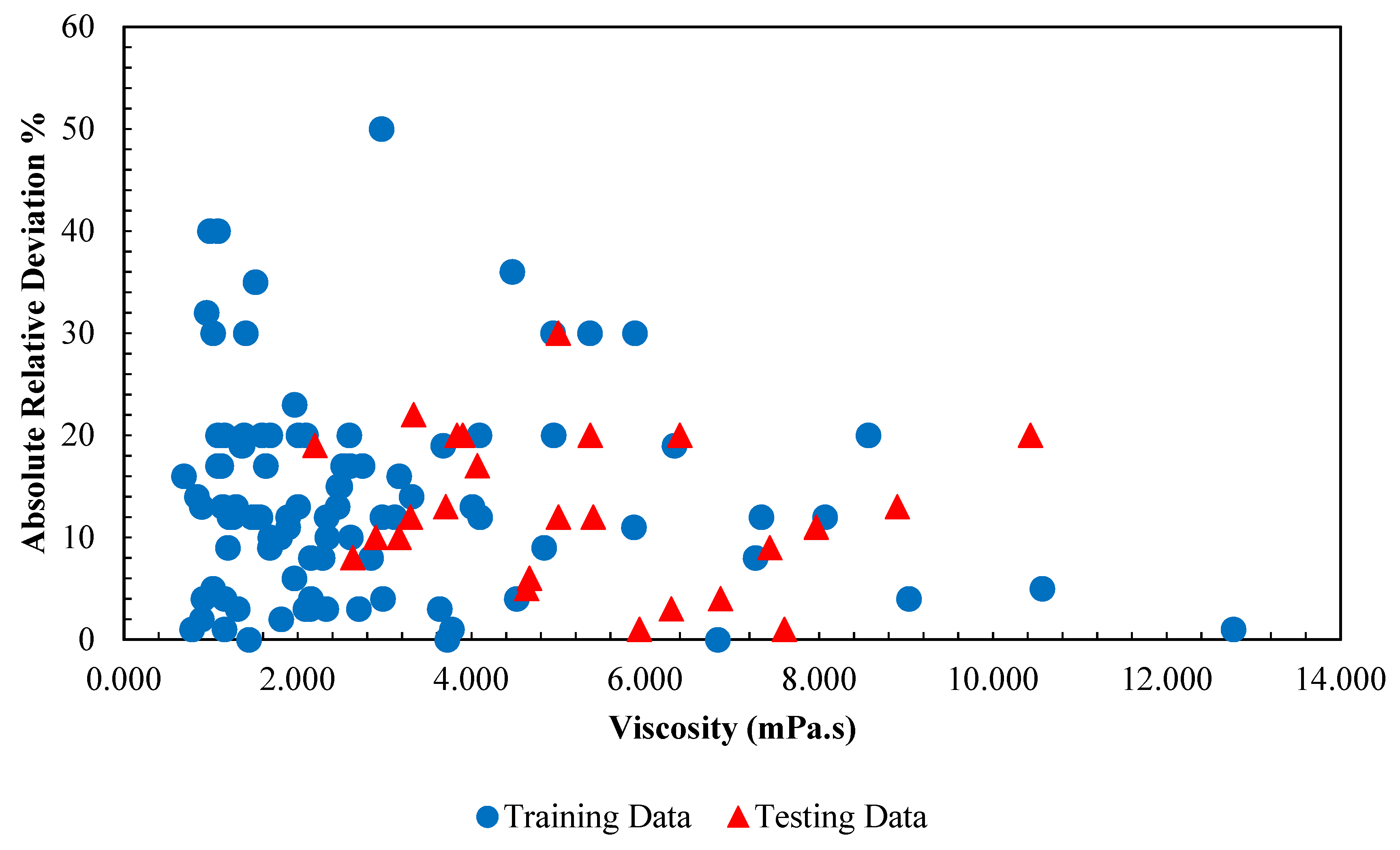
Figure 8.
Absolute relative error distribution of the obtained outputs from LSSVM model versus corresponding viscosity of /ethylene glycol-water nanofluid data points.
Figure 8.
Absolute relative error distribution of the obtained outputs from LSSVM model versus corresponding viscosity of /ethylene glycol-water nanofluid data points.
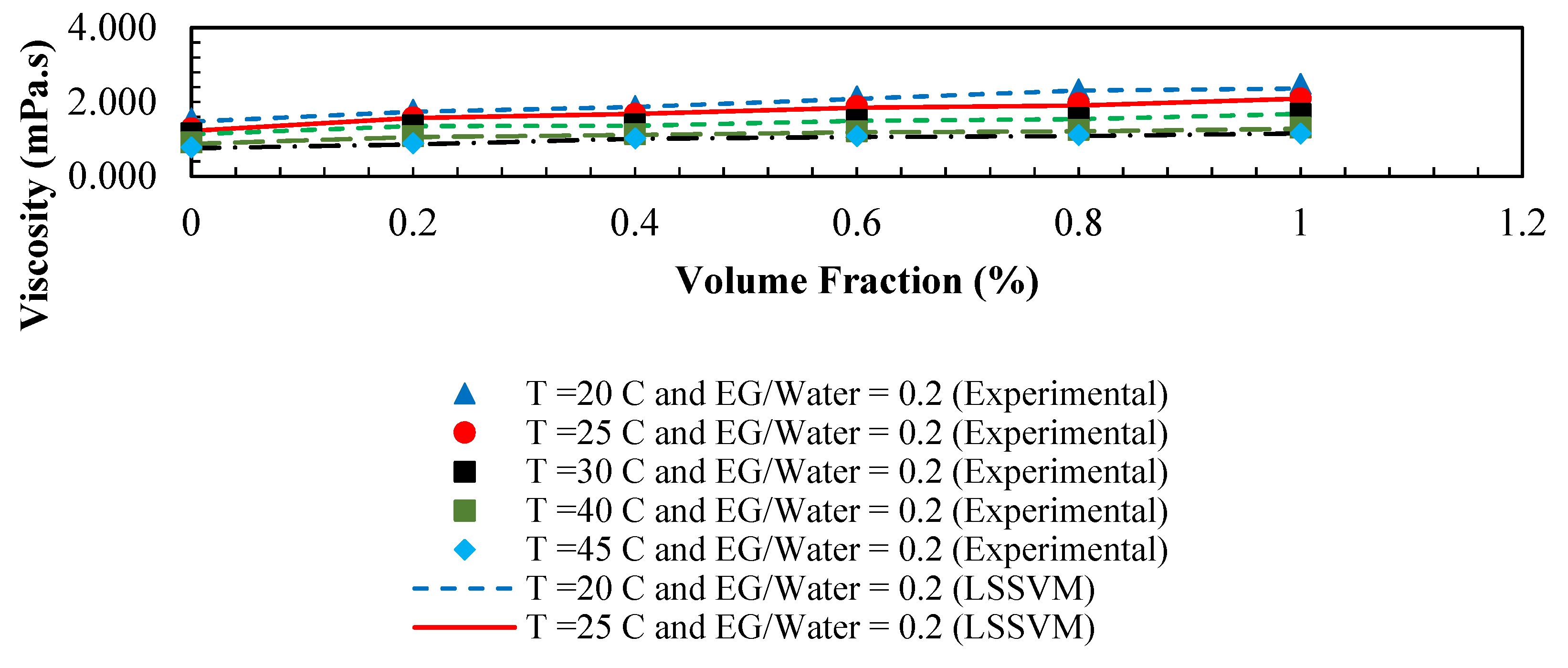
Figure 9.
Comparison between predicted and experimental viscosity of /ethylene glycol-water nanofluid, versus volume fraction (%) at different condition.
Figure 9.
Comparison between predicted and experimental viscosity of /ethylene glycol-water nanofluid, versus volume fraction (%) at different condition.
Figure 10.
Relative importance of each input variables on the viscosity of /ethylene glycol-water nanofluid.
Figure 10.
Relative importance of each input variables on the viscosity of /ethylene glycol-water nanofluid.
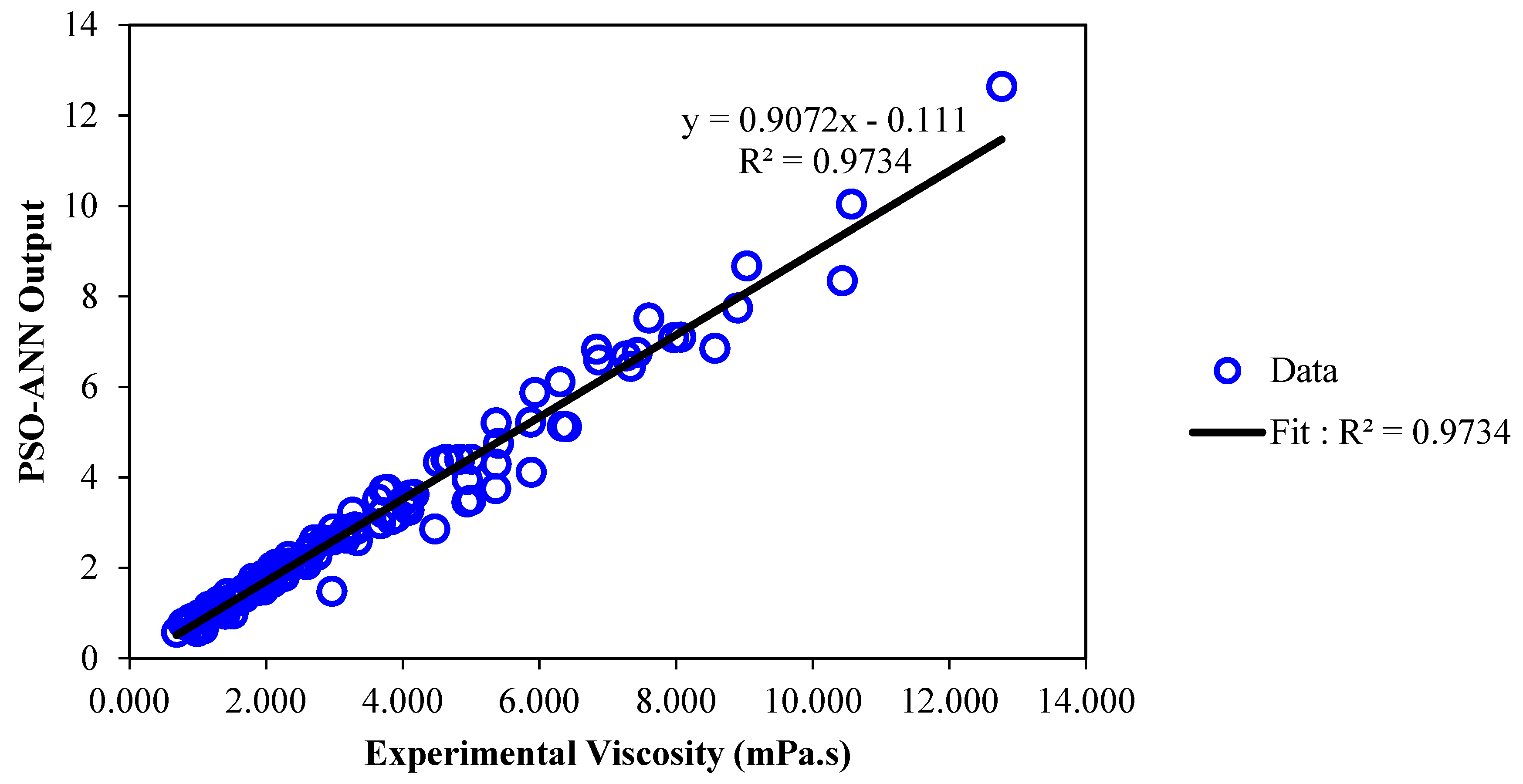
Figure 11.
Regression plot of the proposed PSO-ANN model versus actual viscosity of /ethylene glycol-water nanofluid.
Figure 11.
Regression plot of the proposed PSO-ANN model versus actual viscosity of /ethylene glycol-water nanofluid.
Figure 12.
Comparison between actual viscosity of /ethylene glycol-water nanofluid and predicted values by PSO-ANN model versus relevant data index.
Figure 12.
Comparison between actual viscosity of /ethylene glycol-water nanofluid and predicted values by PSO-ANN model versus relevant data index.
Figure 13.
Absolute relative error distribution of the obtained outputs from PSO-ANN model versus corresponding viscosity of /ethylene glycol-water nanofluid data points.
Figure 13.
Absolute relative error distribution of the obtained outputs from PSO-ANN model versus corresponding viscosity of /ethylene glycol-water nanofluid data points.
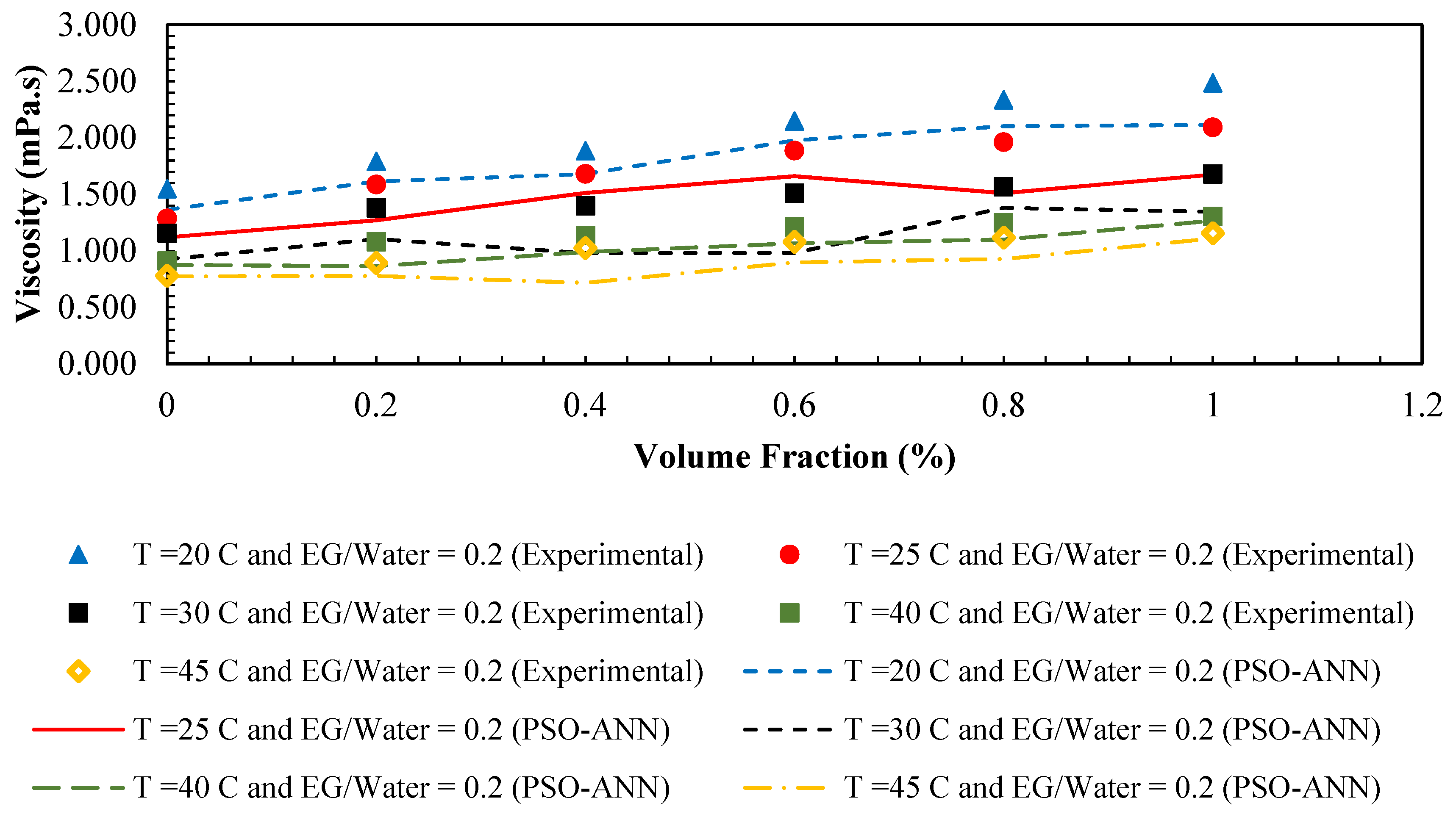
Figure 14.
Comparison between PSO-ANN outputs and experimental viscosity of /ethylene glycol-water nanofluid, versus volume fraction (%) at different condition.
Figure 14.
Comparison between PSO-ANN outputs and experimental viscosity of /ethylene glycol-water nanofluid, versus volume fraction (%) at different condition.
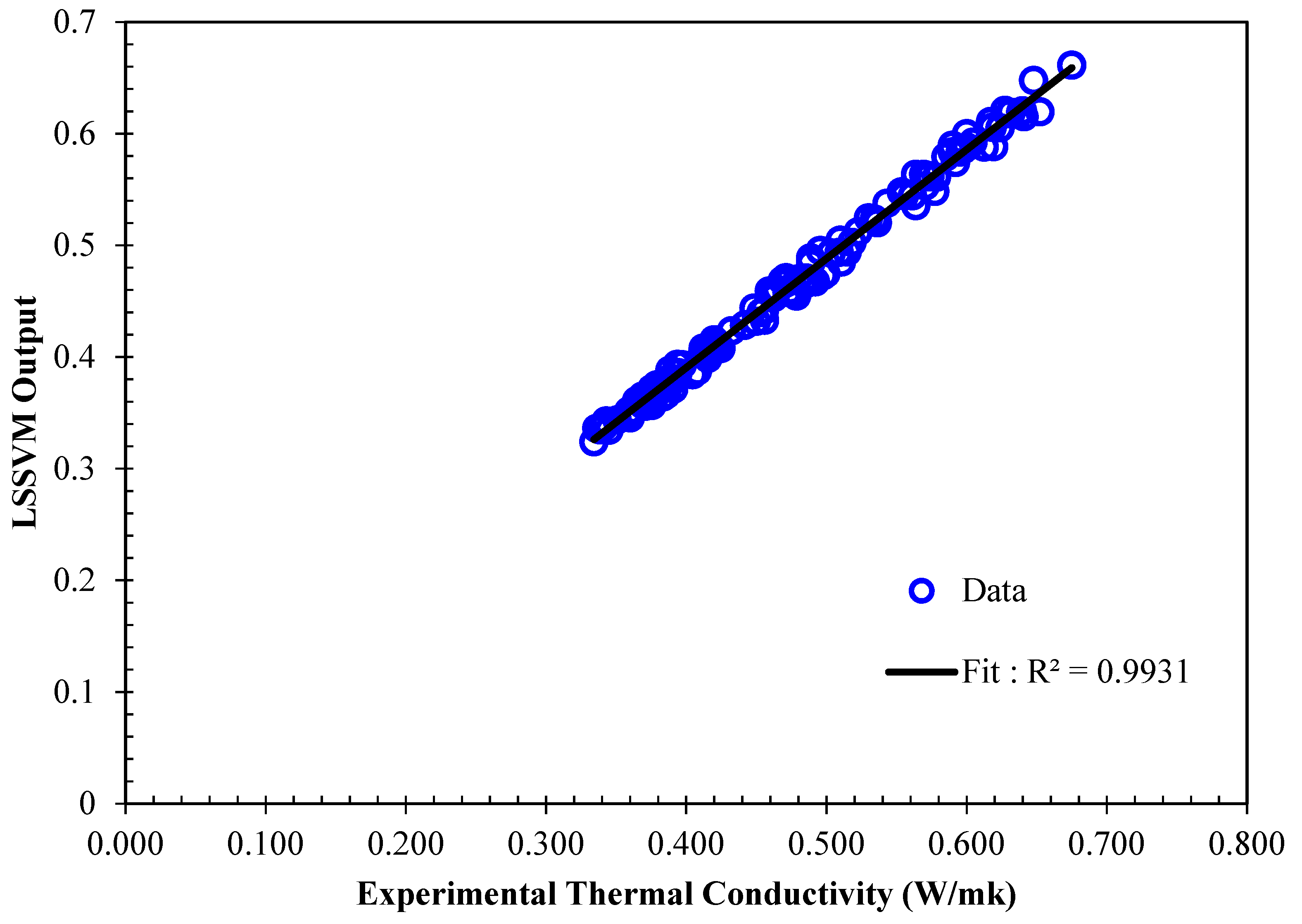
Figure 15.
Regression plot of the proposed vector machine model versus actual thermal conductivity of /ethylene glycol-water nanofluid.
Figure 15.
Regression plot of the proposed vector machine model versus actual thermal conductivity of /ethylene glycol-water nanofluid.
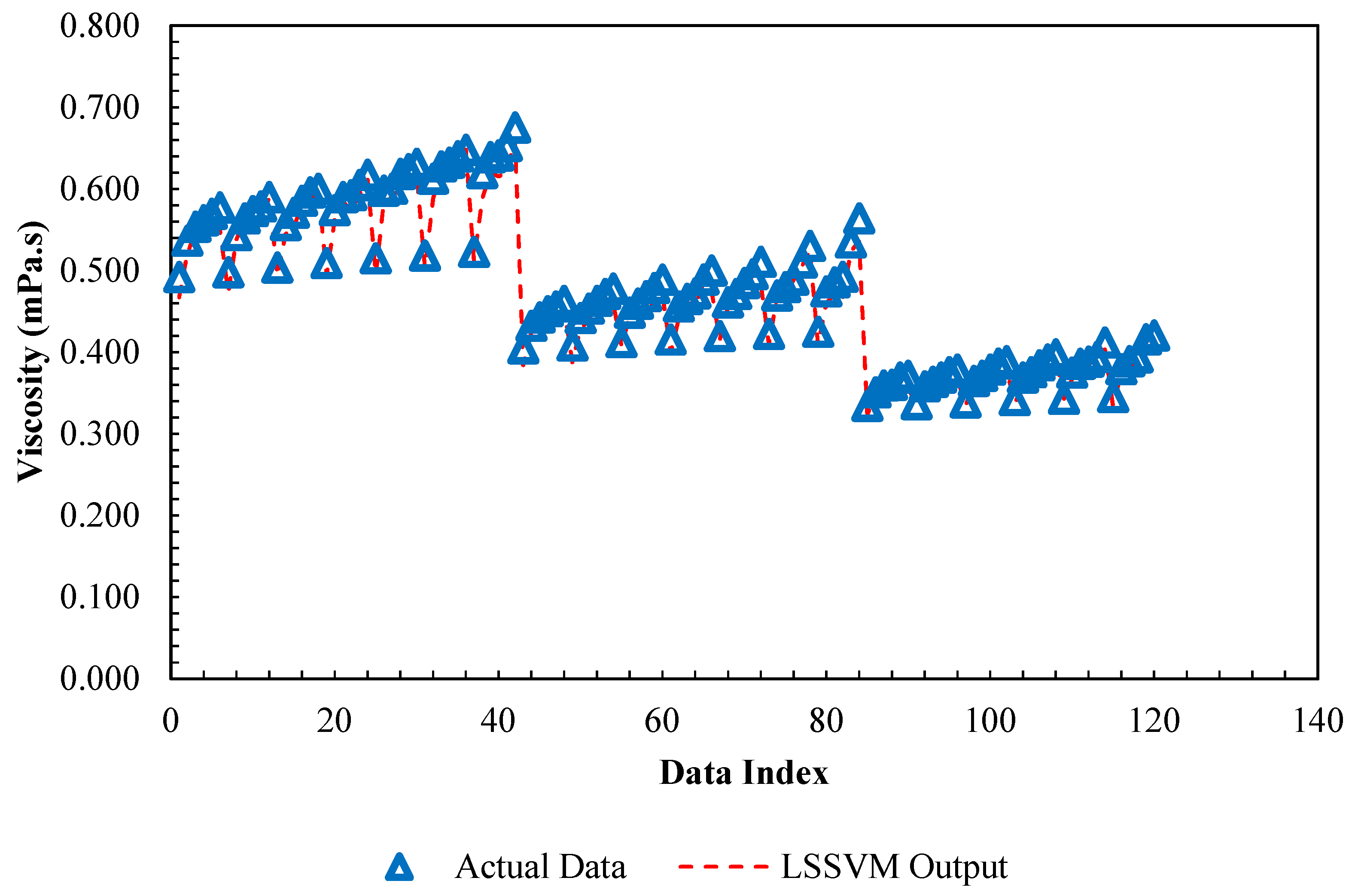
Figure 16.
Comparison between actual thermal conductivity of /ethylene glycol-water nanofluid and predicted values by LSSVM model versus relevant data index.
Figure 16.
Comparison between actual thermal conductivity of /ethylene glycol-water nanofluid and predicted values by LSSVM model versus relevant data index.
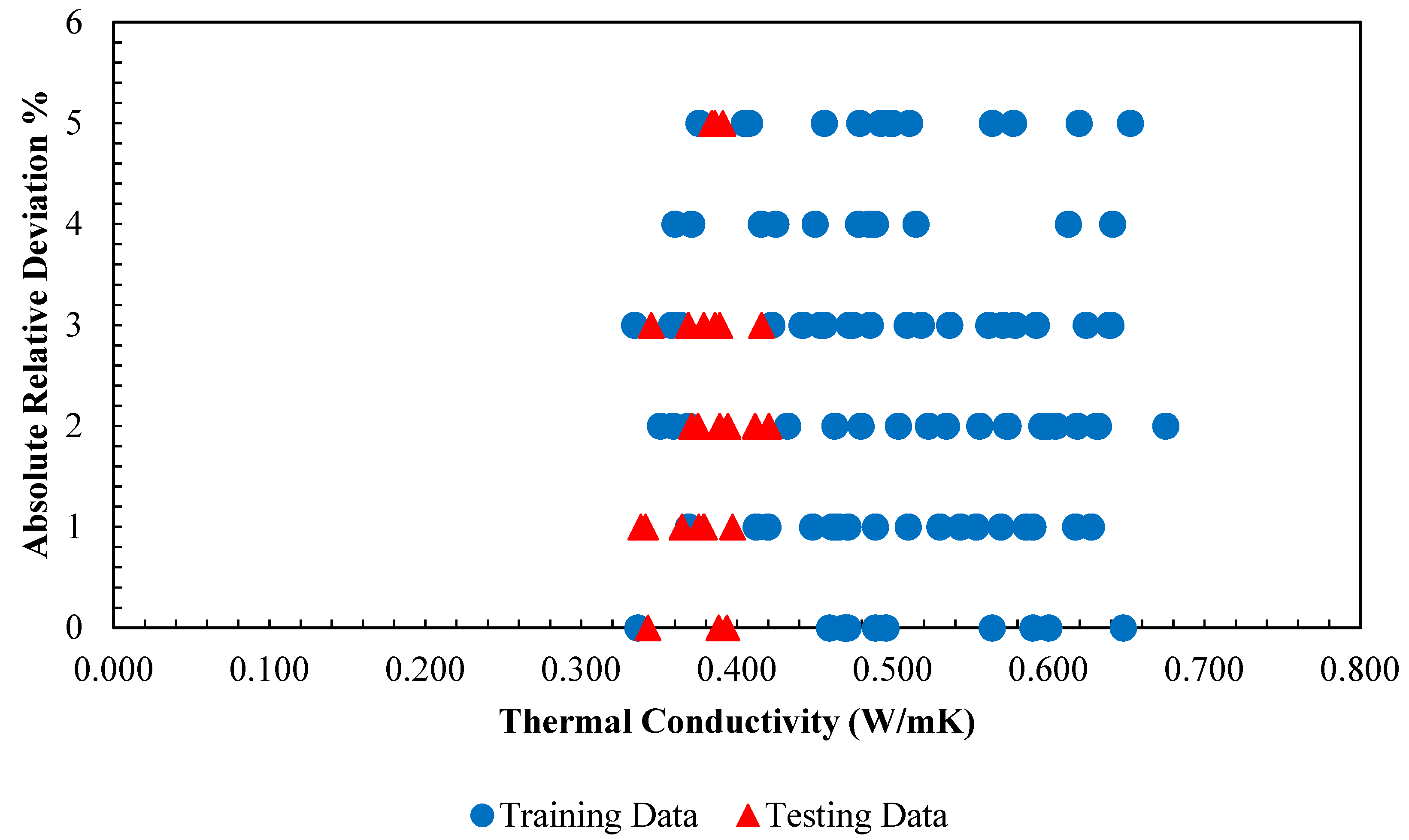
Figure 17.
Absolute relative error distribution of the obtained outputs from LSSVM model versus corresponding thermal conductivity of /ethylene glycol-water nanofluid data points.
Figure 17.
Absolute relative error distribution of the obtained outputs from LSSVM model versus corresponding thermal conductivity of /ethylene glycol-water nanofluid data points.
Figure 18.
Comparison between predicted and experimental thermal conductivity of /ethylene glycol-water mixture, versus volume fraction (%) at different condition.
Figure 18.
Comparison between predicted and experimental thermal conductivity of /ethylene glycol-water mixture, versus volume fraction (%) at different condition.
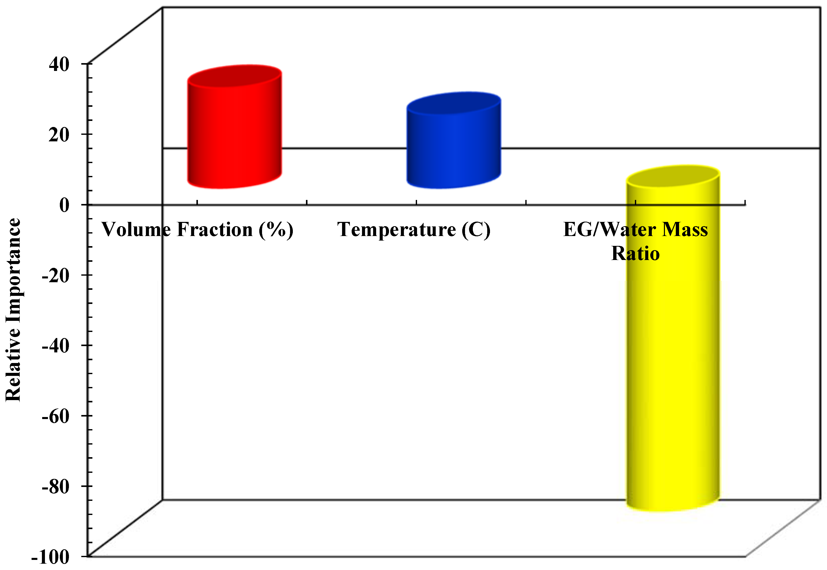
Figure 19.
Relative importance of each input variables on the thermal conductivity of /ethylene glycol-water nanofluid.
Figure 19.
Relative importance of each input variables on the thermal conductivity of /ethylene glycol-water nanofluid.
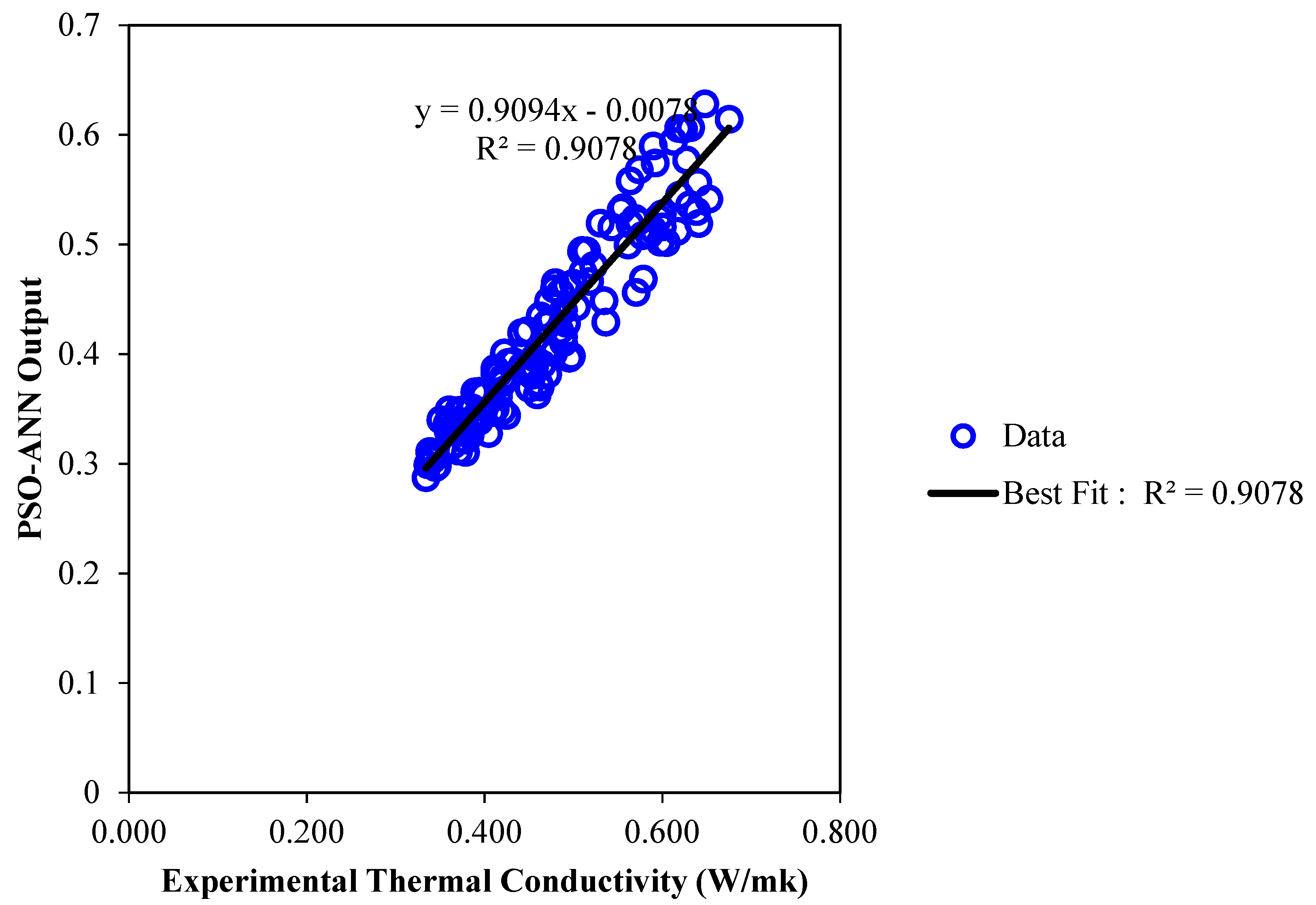
Figure 20.
Regression plot of the proposed PSO-ANN model versus actual thermal conductivity of /ethylene glycol-water nanofluid.
Figure 20.
Regression plot of the proposed PSO-ANN model versus actual thermal conductivity of /ethylene glycol-water nanofluid.
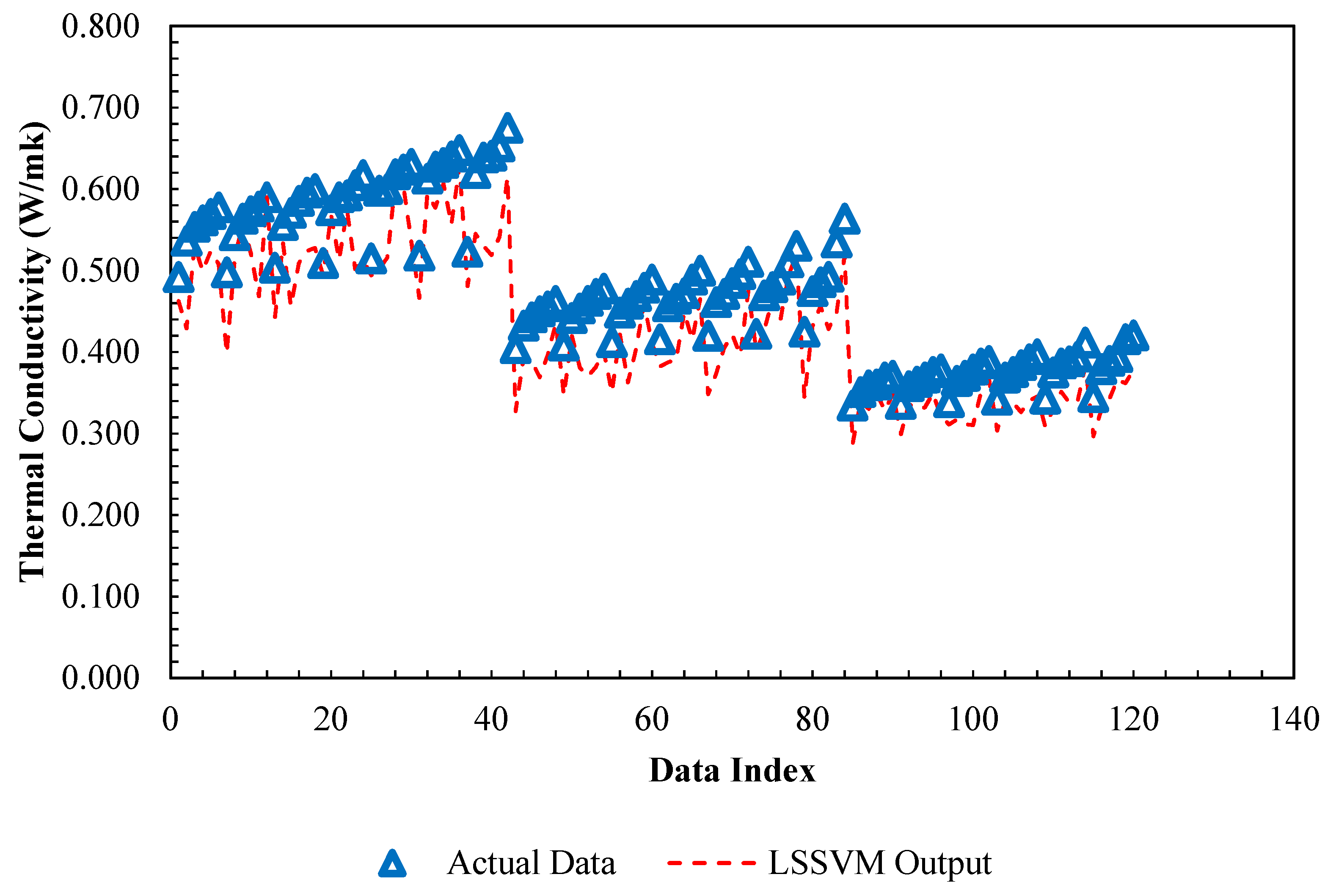
Figure 21.
Comparison between actual thermal conductivity of /ethylene glycol-water nanofluid and predicted values by PSO-ANN model versus relevant data index.
Figure 21.
Comparison between actual thermal conductivity of /ethylene glycol-water nanofluid and predicted values by PSO-ANN model versus relevant data index.
Figure 22.
Absolute relative error distribution of the obtained outputs from PSO-ANN model versus corresponding thermal conductivity of /ethylene glycol-water nanofluid data points.
Figure 22.
Absolute relative error distribution of the obtained outputs from PSO-ANN model versus corresponding thermal conductivity of /ethylene glycol-water nanofluid data points.
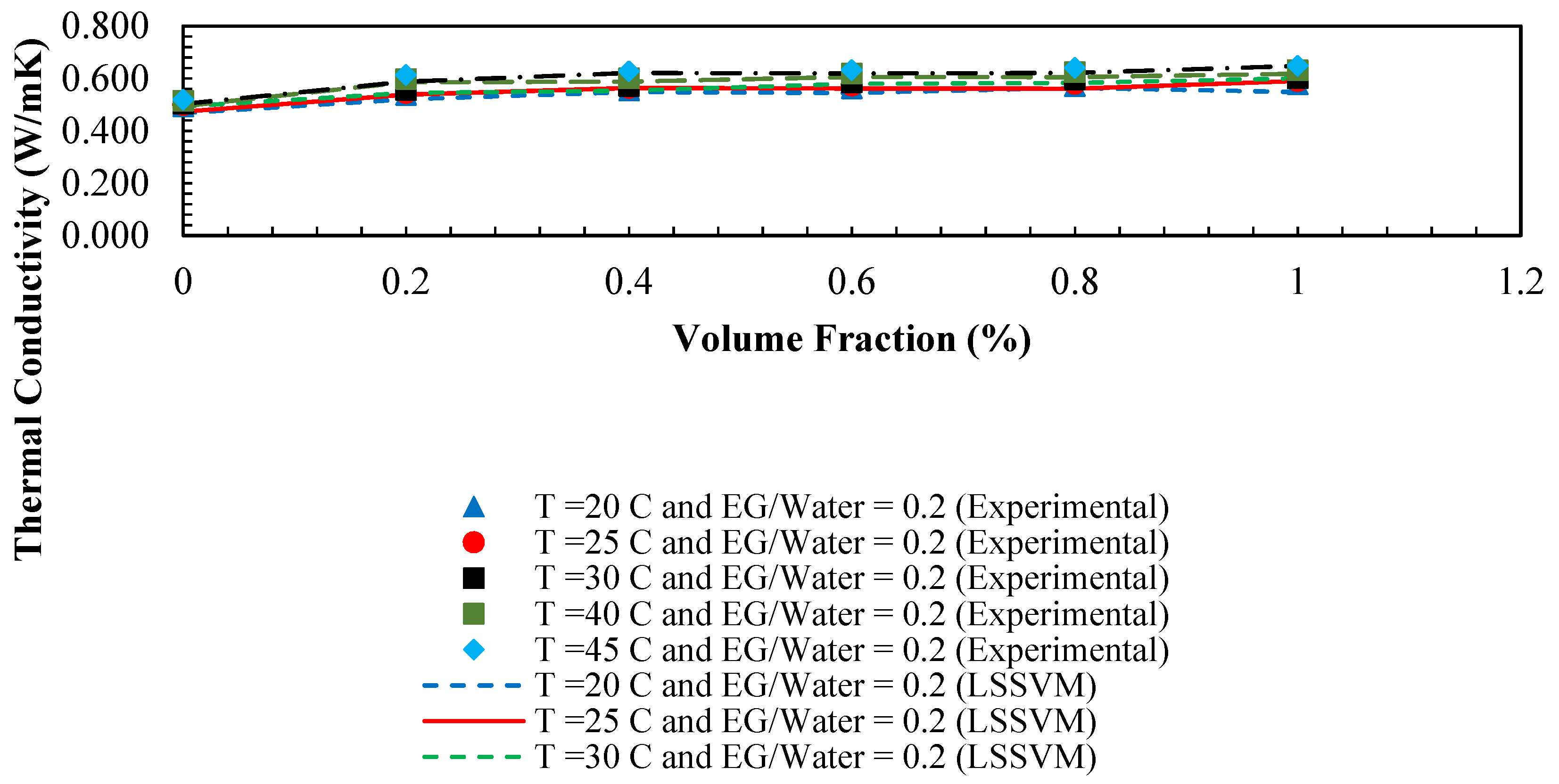
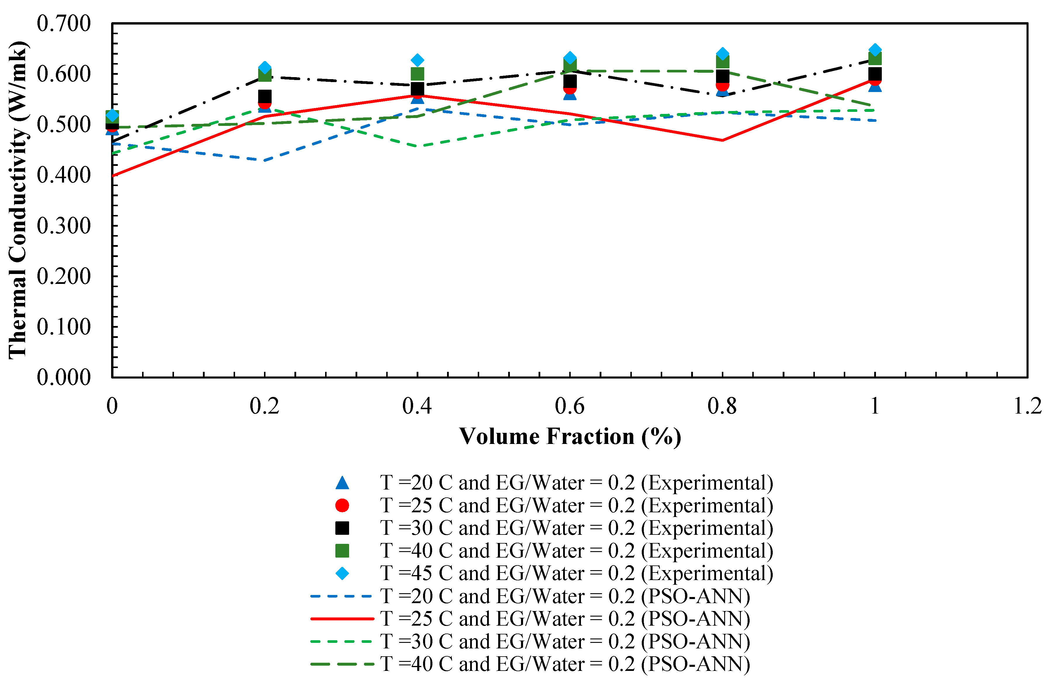
Figure 23.
Comparison between PSO-ANN outputs and experimental thermal conductivity of /ethylene glycol-water nanofluid, versus volume fraction (%) at different condition.
Figure 23.
Comparison between PSO-ANN outputs and experimental thermal conductivity of /ethylene glycol-water nanofluid, versus volume fraction (%) at different condition.
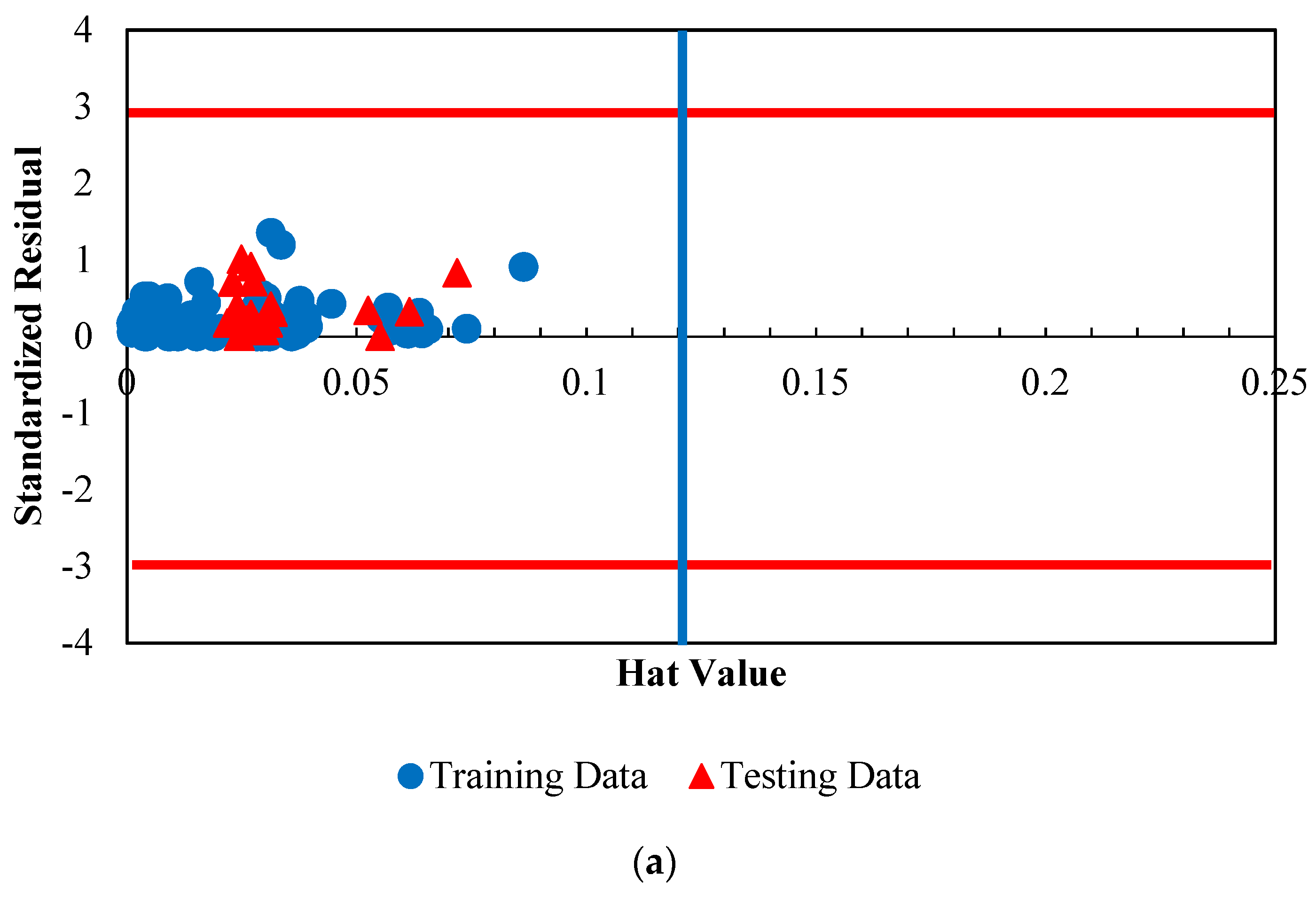
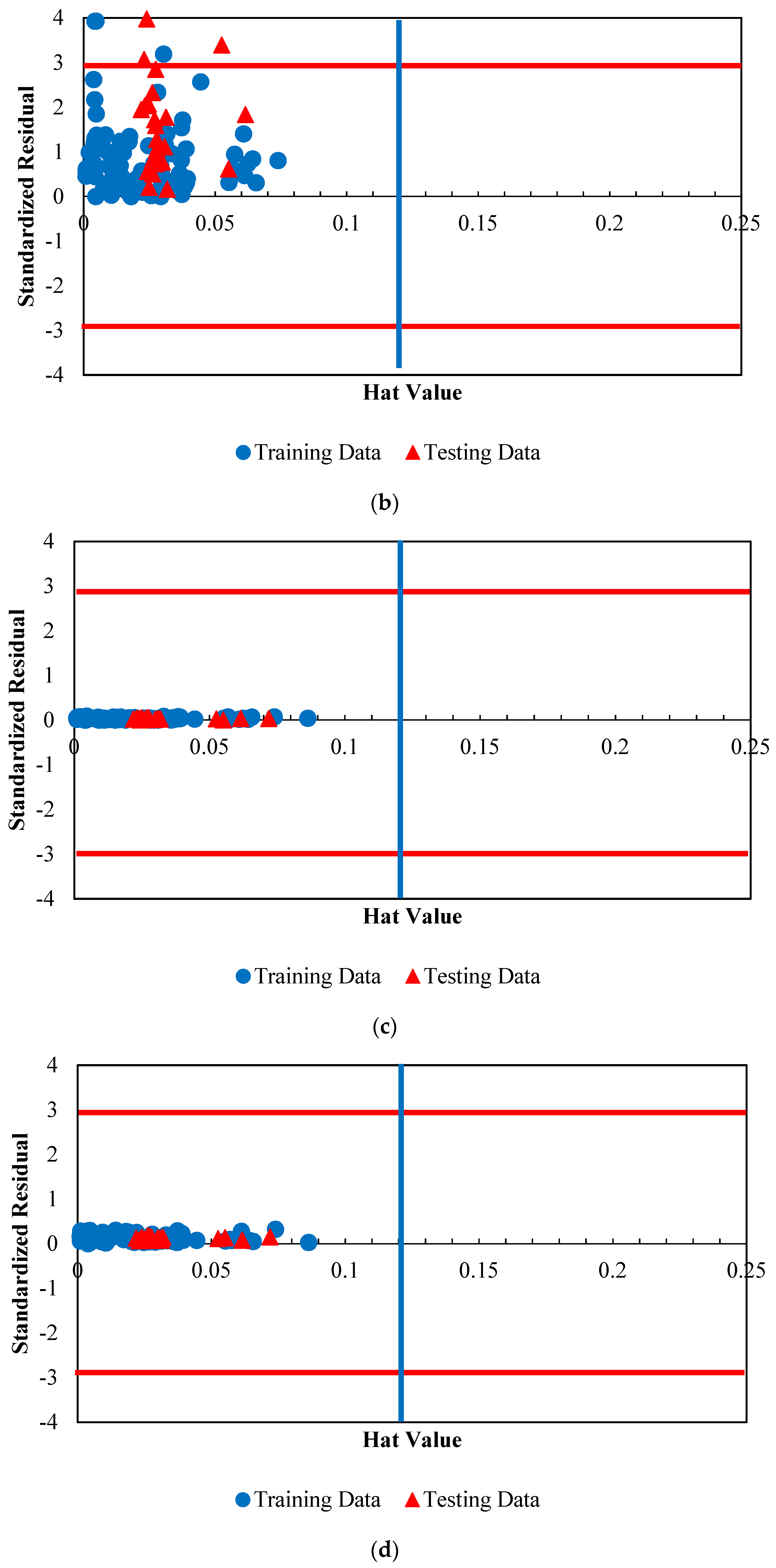
Figure 24.
Detection of the probable doubtful measured viscosity and thermal conductivity data and the applicability domain of the suggested approaches for the viscosity of /ethylene glycol-water nanofluid. (a) GA-LSSVM model for viscosity prediction (b) PSO-ANN model for viscosity prediction (c) GA-LSSVM model for thermal conductivity prediction (d) PSO-ANN model for thermal conductivity prediction (the H* value is 0.12).
Table 1.
Details of trained ANNs with PSO for the prediction of viscosity and thermal conductivity of /ethylene glycol-water nanofluid.
Table 1.
Details of trained ANNs with PSO for the prediction of viscosity and thermal conductivity of /ethylene glycol-water nanofluid.
| Type | Value/Comment |
|---|
| Input layer | 3 |
| Hidden layer | 8 |
| Output layer | 2 |
| Hidden layer activation function | Logsig |
| Output layer activation function | Purelin |
| Number of datum used for training | 100 |
| Number of datum used for testing | 26 |
| Number of max iterations | 1000 |
| c1 and c2 in Equation (15) | 2 |
| Number of particles | 25 |
Table 2.
Basic parameter values of GA-LSSVM model for the prediction of viscosity and thermal conductivity of /ethylene glycol-water nanofluid.
Table 2.
Basic parameter values of GA-LSSVM model for the prediction of viscosity and thermal conductivity of /ethylene glycol-water nanofluid.
| Type | Value/Comment |
|---|
| Input layer | 2 |
| Output layer | 1 |
| Kernel function | RBF kernel function |
| Number of datum used for training | 100 |
| Number of datum used for testing | 26 |
| GA Population size | 1000 |
| Max. number of generations | 1000 |
| Crossover rate | 0.82 |
| Mutation rate | 0.02 |
Table 3.
Statistical parameters of the evolved LSSVM approach for determination of viscosity of /ethylene glycol-water nanofluid.
Table 3.
Statistical parameters of the evolved LSSVM approach for determination of viscosity of /ethylene glycol-water nanofluid.
| Training Set |
| R2 | 0.9995 |
| Average absolute relative deviation | 2.8194 |
| mean square error | 0.01387 |
| N | 100 |
| Test Set |
| R2 | 0.9985 |
| Average absolute relative deviation | 2.1923 |
| mean square error | 0.433 |
| N | 26 |
| Total |
| R2 | 0.9993 |
| Average absolute relative deviation | 2.7828 |
| mean square error | 0.0156 |
| N | 126 |
Table 4.
Calculated statistical indexes of the implemented intelligence-based approaches for the viscosity of /ethylene glycol-water mixture determination.
Table 4.
Calculated statistical indexes of the implemented intelligence-based approaches for the viscosity of /ethylene glycol-water mixture determination.
| Statistical Parameter | LSSVM | PSO-ANN |
|---|
| (MSE) | 0.0156 | 0.3541 |
| R2 | 0.9993 | 0.9734 |
| AARD | 2.7828 | 13.492 |
Table 5.
Statistical parameters of the evolved LSSVM approach for calculating thermal conductivity of /ethylene glycol-water nanofluid.
Table 5.
Statistical parameters of the evolved LSSVM approach for calculating thermal conductivity of /ethylene glycol-water nanofluid.
| Training Set |
| R2 | 0.9921 |
| Average absolute relative deviation | 2.43 |
| mean square error | 0.00021 |
| N | 100 |
| Test Set |
| R2 | 0.942 |
| Average absolute relative deviation | 2.192 |
| mean square error | 0.0001 |
| N | 26 |
| Total |
| R2 | 0.9931 |
| Average absolute relative deviation | 2.3809 |
| mean square error | 0.00019 |
| N | 126 |
Table 6.
Calculated statistical indexes of the implemented intelligence-based approaches for thermal conductivity of /ethylene glycol-water nanofluid determination.
Table 6.
Calculated statistical indexes of the implemented intelligence-based approaches for thermal conductivity of /ethylene glycol-water nanofluid determination.
| Statistical Parameter | LSSVM | PSO-ANN |
|---|
| (MSE) | 0.00019 | 0.00338 |
| R2 | 0.9931 | 0.9078 |
| AARD | 2.3809 | 10.761 |


 ,
, 


