Article

Offset Free Tracking Predictive Control Based on Dynamic PLS Framework

School of Information and Control Engineering, Liaoning Shihua University, Fushun 113001, China
*
Author to whom correspondence should be addressed.
Information 2017, 8(4), 121; https://doi.org/10.3390/info8040121
Submission received: 30 August 2017 / Revised: 23 September 2017 / Accepted: 25 September 2017 / Published: 10 October 2017

Abstract

:
This paper develops an offset free tracking model predictive control based on a dynamic partial least square (PLS) framework. First, state space model is used as the inner model of PLS to describe the dynamic system, where subspace identification method is used to identify the inner model. Based on the obtained model, multiple independent model predictive control (MPC) controllers are designed. Due to the decoupling character of PLS, these controllers are running separately, which is suitable for distributed control framework. In addition, the increment of inner model output is considered in the cost function of MPC, which involves integral action in the controller. Hence, the offset free tracking performance is guaranteed. The results of an industry background simulation demonstrate the effectiveness of proposed method.

1. Introduction

Nowadays, industrial production is becoming more complex and larger in scale. There are usually hundreds or thousands of input and output variables in this class of novel industrial system. It raises higher requirements for process control technology. With the development of cyber physical systems, more and more new technologies are applied to the industrial process control, such as network control [1], wireless technology [2] and embedded technology [3]. These technologies bring in innovations in the control system, which lead to conventional control theory not being applicable for the application of these new technologies. Model predictive control (MPC) [4] is the most widely used advanced control theory. It has three features: predictive model; rolling optimization, and; feedback correction. Due to the advantages of dealing with multivariable control and constraints [5], MPC has many successful applications. The process of industrial production is sometimes nonlinear. MPC designs for nonlinear system is also one of the hot spots of research. Many research results have formed a special course [6]. Many researchers combine other nonlinear method with MPC such as nonlinear identification [7], neural network [8] and fuzzy model [9] to deal with nonlinear control problem. However, with the increase of dimensionality of controlled variables, the computation load has been greatly increased. MPC is a typical centralized control method, it is not suitable for combing with new cyber physical system technologies such as those mentioned above.
On the other hand, with the development of computation and storage techniques, it became possible to obtain huge dimension and large number of industry production operation data. While the process is often restricted to move in a space of much lower dimension than the data indicate. Hence, many data reduction methods based on principal component extraction are available. Partial least square (PLS) is one of these methods, which is used to model the relationship between two blocks of data. It has been applied to many areas in the past decades, such as quality prediction, process monitoring and chemometrics [10]. PLS is not only able to extract principle component from both the input and output dataset, but also able to determine the direction on which input and output data has the largest covariance [11]. Considering the advantage of dimension reduction and automatic decoupling, many researchers have applied PLS to the modeling and control of dynamic systems. Based on the advantages of PLS, multivariable systems can be decoupled into multiple single input single output (SISO) subsystems. One can design controllers for each subsystem separately, which is suitable for the application of distribute control of cyber physical system. Kaspar and Ray [12,13] proposed a dynamic PLS framework by utilizing the PLS loading matrices to construct precompensators and postcompensatores. Chen and Cheng [14] proposed another dynamic PLS framework with the ARX model. Laurı́ et al. [15] proposed a PLS-based MPC relevant identification method. With these dynamic PLS models (DyPLS), many control schemes are applied. Kaspar and Ray proposed a proportion-integration-differentiation (PID) control scheme under this framework [12], and Chen and Cheng [14] designed multi-loop adaptive PID controllers based on a modified decoupling PLS framework. Hu et al. [16,17] proposed a multi-loop internal model controller in the dynamic PLS framework and achieved better performance for disturbance rejection. LÜ and Liang [18] proposed a multi-loop constrained MPC scheme.
In practice it is often required to track a reference set-point, and achieve zero offset in the presence of persistent disturbances and plant-model mismatch. This type of problem is usually considered as an offset-free problem. To solve this problem, many methods have been proposed so far. One is to augment the state model with disturbance model, which can account for the presence of disturbance or for plant-model mismatch (an observer is usually used). Many algorithms have been developed based on it, for example, references [19,20,21]. González et al. [22] pointed out that if the observer does not reach accurately the stationary state, the model predictions are made on a mistaken stationary model. Another method is to describe the system in the so-called velocity form, see [23,24], where the state is composed by the state increments and the output error, while the manipulated variable is the control increment. The velocity form does not require the use of a state estimator and does not require to compute the steady state target for the plant state and control variables, but no stability results have been established for MPC algorithms based on the velocity form [23]. Pannocchia et al. [25] point out that velocity form model is a special case of disturbance model/observer in the offset-free linear MPC design. A third method is based on the internal model principle. With this method, an integral model is introduced to the system model, and MPC is designed to guarantee the stable of system and integral model. Then the effect of the disturbances is cancelled by the MPC optimization and the controlled variables are tracked at their set-points. This strategy has been followed in [26,27,28,29].
This paper focus on the offset free tracking performance of dynamic PLS control framework, and proposed a novel MPC control strategy. The paper organized as follows. In Section 2, the used dynamic PLS model and its modification are defined and described. Offset-free MPC in DyPLS is described. An industrial background simulation is given to demonstrate the merit of the proposed method. Conclusions are drawn in Section 5.

2. Dynamic PLS Model Description

The origins of PLS are traced to Herman Wold’s original non-linear iterative partial least square (NIPALS) algorithm [30]. The advantage of PLS lies in that it decomposes the multivariate regression problem into a series of uncorrelated univariate regression problems, and problems of non-square and ill-conditioned in the regression can be dealt with [11]. The conventional PLS consists of an outer model which extracts the latent variables, and an inner model to estimate the algebraic relationship between the input and output scores [31]. Considering scaled l × m dimension input dataset X and a l × n dimension output dataset Y, where l, m and n denote the number of sampling, input dimension and output dimension, respectively. The outer model is built by decomposing matrix X and Y as follows:
X = r = 1 R t r p r T + E * = T P T + E * Y = r = 1 R u r q r T + F * = U Q T + F *
where R is the number of latent variables (due to the effect of dimensionality reduction of PLS. R max ( m , n ) is met in most cases), pr and qr are the r-th loading vectors of loading matrices P and Q, respectively; t r and u r are the r-th score vectors of matrices T and U, respectively; and E* and F* are residual matrices of X and Y, respectively.
In inner model, the score matrices T and U are related by a diagonal matrix B (Equation (2)) which is obtained by least squares (LS) method.
u r = b r t r U = T B
where, b r = u r T t r t r T t r ; B = ( T T T ) 1 T T U ; U = diag ( u 1 , u 2 , , u R ) ; T = diag ( t 1 , t 2 , , t R ) .
The conventional PLS is suitable for pure algebraic regression. It is not able to cope with dynamic system such as industry process systems. Researchers have proposed many different DyPLS models by introducing dynamic structures into PLS to describe the dynamic character, such as time-series terms [13], dynamic filters [32] or the ARX model [33].
In this paper, state space model is used as PLS inner model to describe the dynamic character. For the r-th latent variable, inner state space model can be expressed as follows:
x r ( k + 1 ) = A r x r ( k ) + B r t r ( k ) u r ( k ) = C r x r ( k )
The state space model can be obtained by subspace identification method [34], and the dimension of parameters Ar, Br, Cr can be determined by model output error method. The structure of dynamic PLS with state space model is shown in Figure 1, where, Wx and Wy are scaling matrices of X and Y.

3. Predictive Controller Design

3.1. Dynamic PLS Control Framework

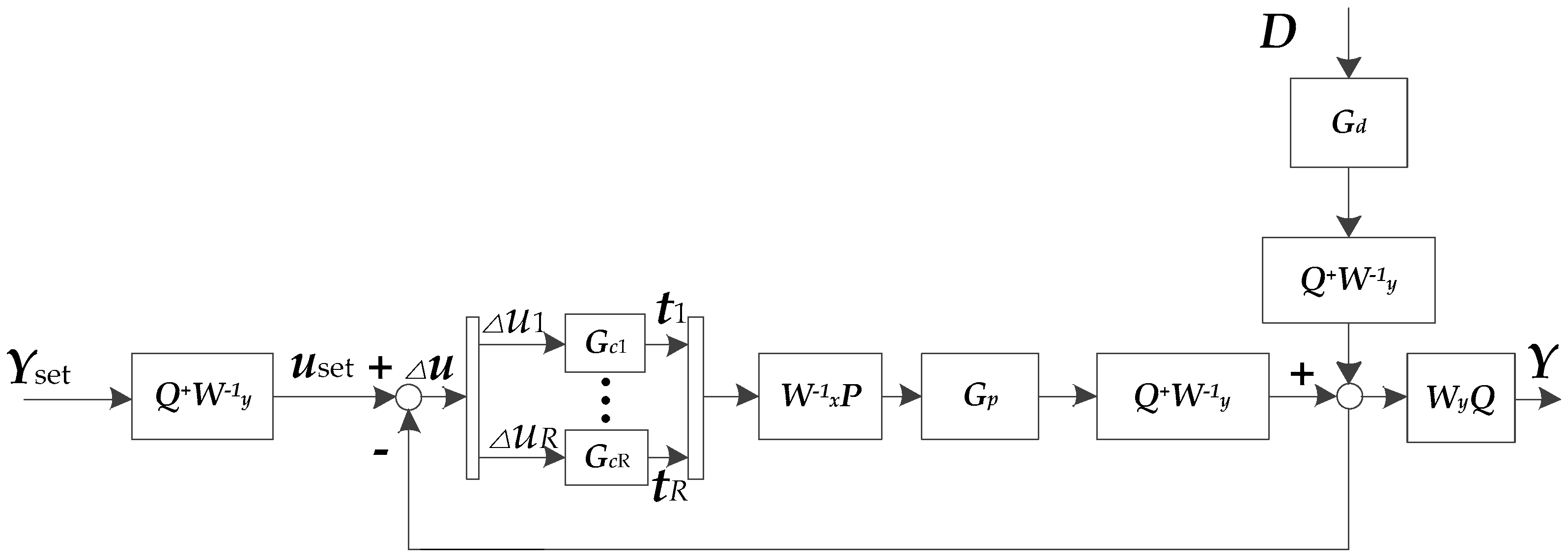
Shown in Figure 2 is the control structure with dynamic PLS model proposed by Kaspar and Ray [13]. Based on the DyPLS model proposed in Section 2, this scheme employs the PLS loading matrices P and Q as precompensators and postcompensators to connect the actual process. With the loading matrices, inputs and outputs of the system are mapped into the latent variable space. Controllers designed in the latent variable space use input scores to control output scores. Since the multiple input multiple output (MIMO) system is decoupled into multiple single input single output (SISO) subsystems in latent variable space, the original MIMO controller problem is decomposed into multiple independent SISO control problems. A variety of conventional controls scheme could be involved in this control framework [13]. In this framework, each controller in the latent variable space responds synchronously to the error between score variable u and its set-point, which is Yset mapped into the latent variable space. Generated controller output T is back mapped into origin space and then is used as the input of the system.
In Figure 2, G c i ( i = 1 , , R ) , Gp and Gd are the transfer function matrices of the controller in latent variable space, the controlled plant and disturbances, respectively; Q+ is the appropriate inverse of Q. Yset is the set-point sequence of process; D is the disturbance sequence. Δ = 1 z 1 .

3.2. Equation of Prediction

The r-th inner model Equation (3) can be considered in incremental forms as follows:
Δ x r ( k + 1 ) = A r Δ x r ( k ) + B r Δ t r ( k ) Δ u r ( k ) = C r Δ x r ( k )
Let Np,r and Nc,r denote prediction horizon and control horizon for the r-th controller, respectively.
Considering Equation (3), the Np,r step ahead prediction of state with Nc,r control step are
[ x ^ r ( k + 1 | k ) x ^ r ( k + N c , r | k ) x ^ r ( k + N c , r + 1 | k ) x ^ r ( k + N p , r | k ) ] = [ A r A r N c , r A r N c , r + 1 A r N p , r ] x r ( k ) + [ B r i = 0 N c , r 1 A r i B r i = 0 N c , r A r i B r i = 0 N p , r 1 A r i B r ] t r ( k 1 ) + [ B r 0 i = 0 N c , r 1 A r i B r B r i = 0 N c , r A r i B r i = 0 1 A r i B r i = 0 N p , r 1 A r i B r i = 0 N p , r N c , r A r i B r ] [ Δ t ^ r ( k | k ) Δ t ^ r ( k + N c , r 1 | k ) ]
Similarly, with Equation (4), the Np,r step ahead prediction of incremental state with Nc,r control step are
[ Δ x ^ r ( k + 1 | k ) Δ x ^ r ( k + N c , r | k ) Δ x ^ r ( k + N c , r + 1 | k ) Δ x ^ r ( k + N p , r | k ) ] = [ A r A r N c , r A r N c , r + 1 A r N p , r ] x r ( k ) + [ B r 0 i = 0 N c , r 1 A r i B r B r i = 0 N c , r A r i B r i = 0 1 A r i B r i = 0 N p , r 1 A r i B r i = 0 N p , r N c , r A r i B r ] [ Δ t ^ r ( k | k ) Δ t ^ r ( k + N c , r 1 | k ) ]
From Equation (5) and considering Equation (3), the estimates of future of inner model output are
[ u ^ r ( k + 1 | k ) u ^ r ( k + N c , r | k ) u ^ r ( k + N c , r + 1 | k ) u ^ r ( k + N p , r | k ) ] = [ C r A r C r A r N c , r C r A r N c , r + 1 C r A r N p , r ] x r ( k ) + [ C r B r i = 0 N c , r 1 C r A r i B r i = 0 N c , r C r A r i B r i = 0 N p , r 1 C r A r i B r ] t r ( k 1 ) + [ C r B r 0 i = 0 N c , r 1 C r A r i B r C r B r i = 0 N c , r C r A r i B r i = 0 1 C r A r i B r i = 0 N p , r 1 C r A r i B r i = 0 N p , r N c , r C r A r i B r ] [ Δ t ^ r ( k | k ) Δ t ^ r ( k + N c , r 1 | k ) ]
Equation (7) can be written in matrix notation as follows:
u ^ r ( k ) = Φ r x r ( k ) + Ψ r u r ( k ) + Γ r Δ t ^ r ( k )
where u ^ r ( k ) = [ u ^ r ( k + 1 | k ) , , u ^ r ( k + N p , r | k ) ] T , Δ t ^ r ( k ) = [ Δ t ^ r ( k | k ) , , Δ t ^ r ( k + N c , r 1 | k ) ] T , Φ r = [ C r A r , C r A r N p , r ] T , Ψ r = [ C r B r , , i = 0 N p , r 1 C r A r i B r ] T , Γ r = [ C r B r 0 i = 0 N c , r 1 C r A r i B r C r B r i = 0 N c , r C r A r i B r i = 0 1 C r A r i B r i = 0 N p , r 1 C r A r i B r i = 0 N p , r N c , r C r A r i B r ] .
Similarly, from Equation (6) and considering Equation (4), the estimates of future of inner model output are
[ Δ u ^ r ( k + 1 | k ) Δ u ^ r ( k + N c , r | k ) Δ u ^ r ( k + N c , r + 1 | k ) Δ u ^ r ( k + N p , r | k ) ] = [ C r A r C r A r N c , r C r A r N c , r + 1 C r A r N p , r ] x r ( k ) + [ C r B r 0 i = 0 N c , r 1 C r A r i B r C r B r i = 0 N c , r C r A r i B r i = 0 1 C r A r i B r i = 0 N p , r 1 C r A r i B r i = 0 N p , r N c , r C r A r i B r ] [ Δ t ^ r ( k | k ) Δ t ^ r ( k + N c , r 1 | k ) ]
Equation (9) can be written in matrix notation as follows:
Δ u ^ r ( k ) = Φ r Δ x r ( k ) + Γ r Δ t ^ r ( k )
where Δ u ^ r ( k ) = [ Δ u ^ r ( k + 1 | k ) , , Δ u ^ r ( k + N p , r | k ) ] T .

3.3. Offset-Free Control

In order to get offset-free tracking performance, it should give zero value for the error between set-point and system output as
lim k e ( k ) = lim k u set r ( k ) u r ( k ) 0
According to the final value theorem applied to the control system, it is necessary to provide at least one integrator action in the control loop. A typical cost function of MPC is the 2-norm form as follows:
J r = j = 1 N p , r u set r ( k + j ) u ^ r ( k + j | k ) Q u 2 + j = 1 N c , r Δ t ^ r ( k + j 1 | k ) Q t 2
where u s e t r is the r-th component of uset. Qu and Qt are weighting diagonal matrices. Equation (12) does not add any integrator action. One can modify Equation (12) as follows:
J r = j = 1 N p , r u set r ( k + j ) u ^ r ( k + j | k ) Q u 2 + j = 1 N c , r Δ t ^ r ( k + j 1 | k ) Q t 2 + j = 1 N p , r Δ u ^ r ( k + j | k ) Q Δ u 2
Equation (13) can be written in matrix notation as follows:
J r = u set r u ^ r ( k ) Q u 2 + Δ t ^ r ( k ) Q t 2 + Δ u ^ r ( k ) Q Δ u 2
The cost function Equation (14) contains integrator action for increments Δ u ^ r ( k ) . To optimize the cost function Equation (14), one can get analytical solution of Δ u ^ r ( k ) as
Δ t ^ r ( k ) = [ Γ r T ( Q u + Q Δ u ) Γ r + Q t ] 1 Γ r T [ ( Q u + Q Δ u ) Φ r x r ( k ) Q Δ u Φ r x r ( k 1 ) + Q u ( Ψ r u r ( k ) u set ) ]
One can calculate the control low with Equation (15) offline, so the proposed method will not dramatically increase the online calculation burden. Comparing with conventional MPC, there is only one more polynomial x r ( k 1 ) in the proposed method.
The structure of proposed controller is shown in Figure 3. It is a distributed form which is similar as the distributed model predictive control form [35]. Each controller is a SISO controller, hence the control burden is lower than the conventional MIMO MPC. Hence, this control method is suitable for multiple controllers be embedded in to different low cost control nodes. In each node, there are independent mapping matrices Q + W y 1 and W x 1 P . There is another advantage of this structure. For controllers are operating separately, if one controller is broken down, other controllers can still make the system having a part control action.

3.4. Stability Analysis

Suppose the prediction horizon and control horizon of MPC in latent space are equal, and prediction horizon for different latent variable controllers are also equal. Equation (13) can be reformed as
J r = j = 1 N p u set r ( k + j ) u ^ r ( k + j | k ) Q u 2 + j = 1 N p Δ t ^ r ( k + j 1 | k ) Q t 2 + j = 1 N p Δ u ^ r ( k + j | k ) Q Δ u 2
According to Equations (8) and (13), Equation (16) is a function of state variables and increment input prediction, as
J r = j = 1 N p L ( x ^ r ( k + j | k ) , Δ t ^ r ( k + j 1 | k ) )
Suppose { Δ t ^ r ( k | k ) , , Δ t ^ r ( k + N p 1 | k ) } is the optimal sequence of solution Equation (17). At every time t, Δ t ^ r ( k | k ) is added to control rate at the previous time and acts on the system. Let J r * ( k ) and { x ^ r * ( k | k ) , , x ^ r * ( k + N p 1 | k ) } denote the optimal performance index and optimal state corresponding to this control action. If dynamic PLS can fully describe the actual system and there is no disturbance in system, x r ( k + 1 ) = x ^ r * ( k + 1 | k ) . According to Equation (4), one can get t ^ r ( k + N p | k ) = 0 . When x ^ r ( k + N p | k ) = 0 , then x ^ r ( k + N p + 1 | k ) = 0 . Hence, a feasible control sequence at time t is { Δ t ^ r ( k + 1 | k ) , , Δ t ^ r ( k + N p 1 | k ) , 0 } . A performance index corresponding to it is
J r ( k + 1 ) = J r * ( k ) L ( x ^ r ( k + 1 | k ) , Δ t ^ r ( k | k ) ) J r * ( k )
J r ( k + 1 ) is not less than J r * ( k + 1 ) . Hence
J r * ( k + 1 ) J r * ( k ) L ( x ^ r ( k + 1 | k ) , Δ t ^ r ( k | k ) ) J r * ( k )
Hence, the performance index of each controller in latent space is monotonically decreasing. That is to say that latent output u r ( k ) is bounded. In other words, when k , J r * ( k + 1 ) = J r * ( k ) . According to Equation (1), the system output in original space is a linear combination of u r ( k ) . When u r ( k ) is stable, the original space output is stable.

4. Case Study

The efficiency of the proposed method is demonstrated by carrying out simulation study on polyethylene reaction, which is described by Embirucu and Fontes [36]. Polyethylene is the largest synthetic polymer in terms of production, and stirred-tank reactor is a significant part of it. Ziegler-Natta and Phillips catalysis can be used in this reaction. In these both catalysis, the system is a typical MIMO system with nine inputs and seven outputs. In this study case, Phillips catalysis is chosen. And the first three equations are extracted in this simulation, which are described as follows:
( 1 0.9021 q 1 ) y 1 ( k ) = ( 0.9283 0.8350 q 1 ) x 1 ( k ) ( 1 0.9067 q 1 ) y 2 ( k ) = ( 0.8415 0.7664 q 1 ) x 1 ( k ) + ( 0.6873 0.6023 q 1 ) x 2 ( k ) ( 1 0.8932 q 1 ) y 3 ( k ) = ( 0.8591 0.7536 q 1 ) x 1 ( k ) + ( 0.8097 0.7066 q 1 ) x 3 ( k ) + 0.0081 x 4 ( k )
The description of input and output variables are illustrated in Table 1. This system is a typically non-square system with four inputs and three outputs.
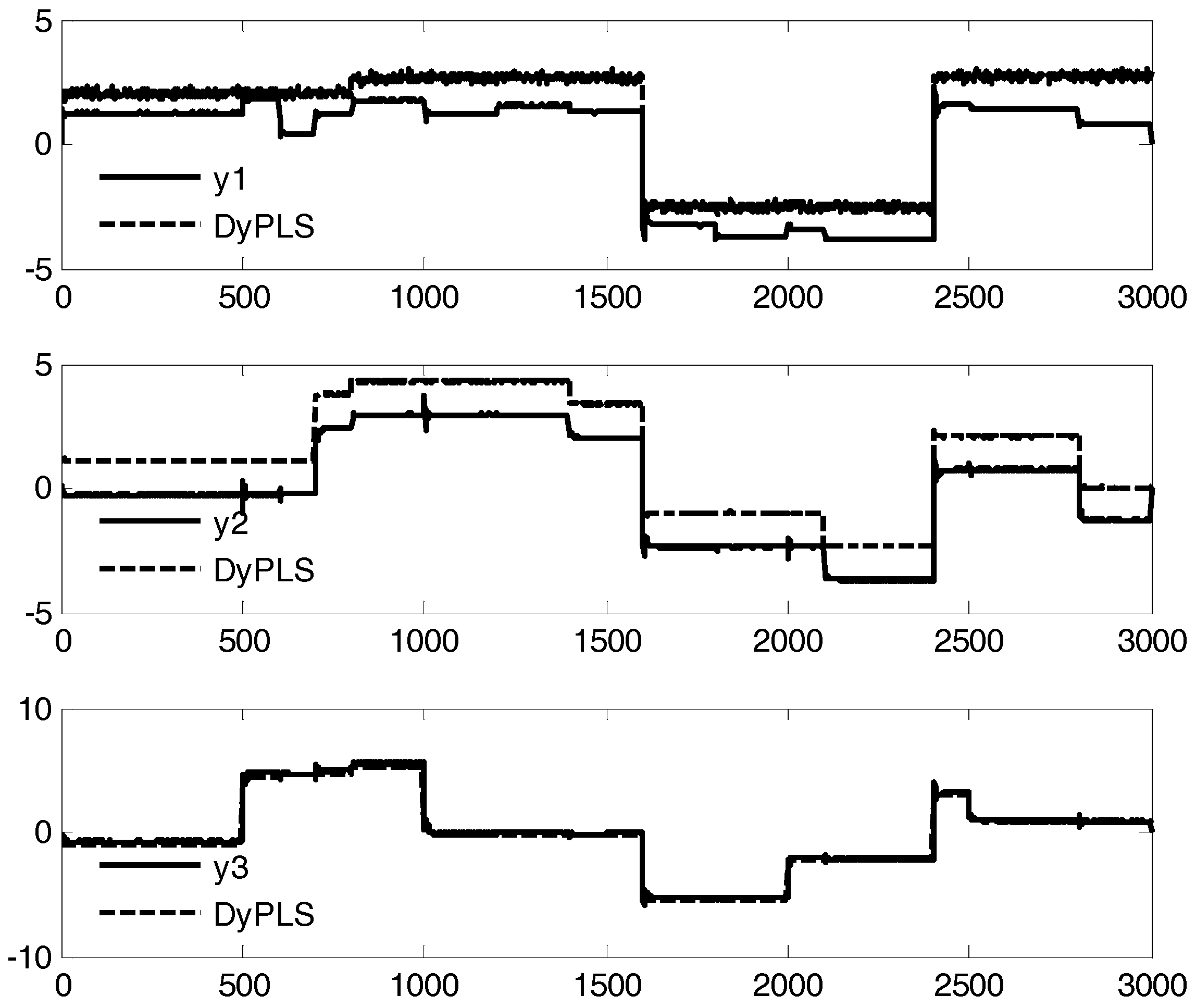
In order to build a well-described dynamic PLS model, four input random step signals magnitudes ranging between −3.5 and 3.5 (shown in Figure 4) are applied to excite the system. In this simulation, a white noise with deviation 0.01 and zero mean is added to input data. The system responses are collected as a part of modeling data (solid line shown in Figure 5). Modeling results are shown in the Figure 5 with dotted line and marked with “DyPLS”. In the DyPLS model, the number of latent variables is three, and the number of state variables of the inner model is five. The integral of squared error between system responses and modeling results of three outputs are 4.2531 × 10 3 , 5.5489 × 10 3 and 243.64, respectively. One can see that the DyPLS did not match process well, that is because some of useful information are ignored due to the iterative modeling mechanism of PLS (according to Equation (1), there is always F* and E*).
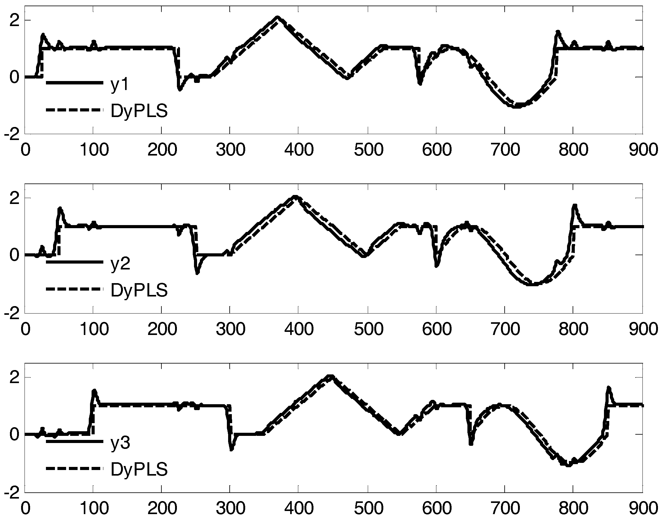
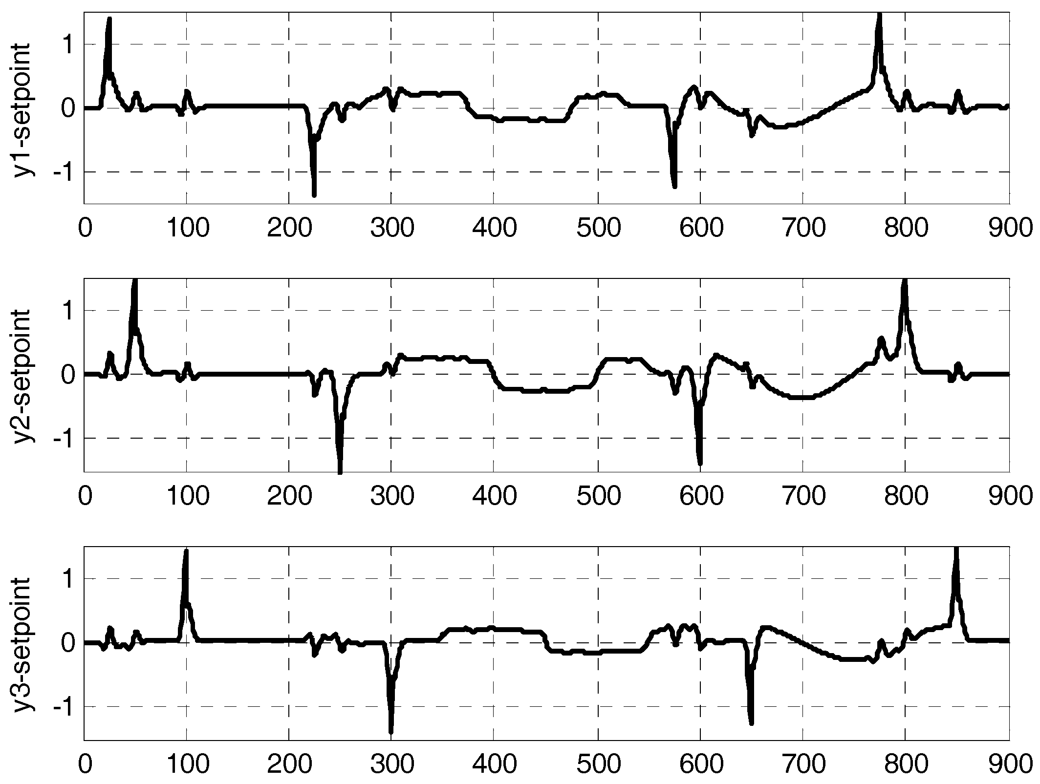
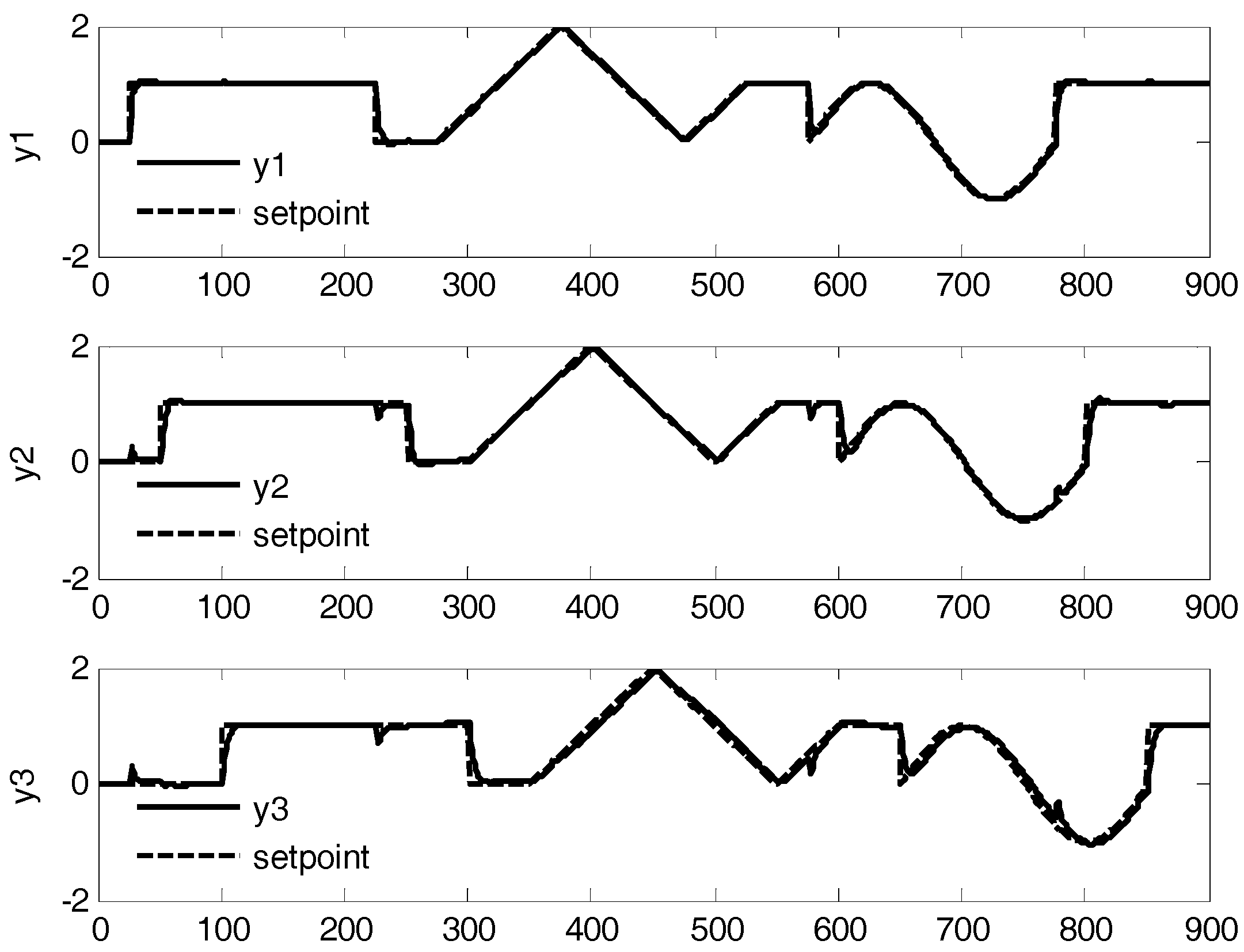
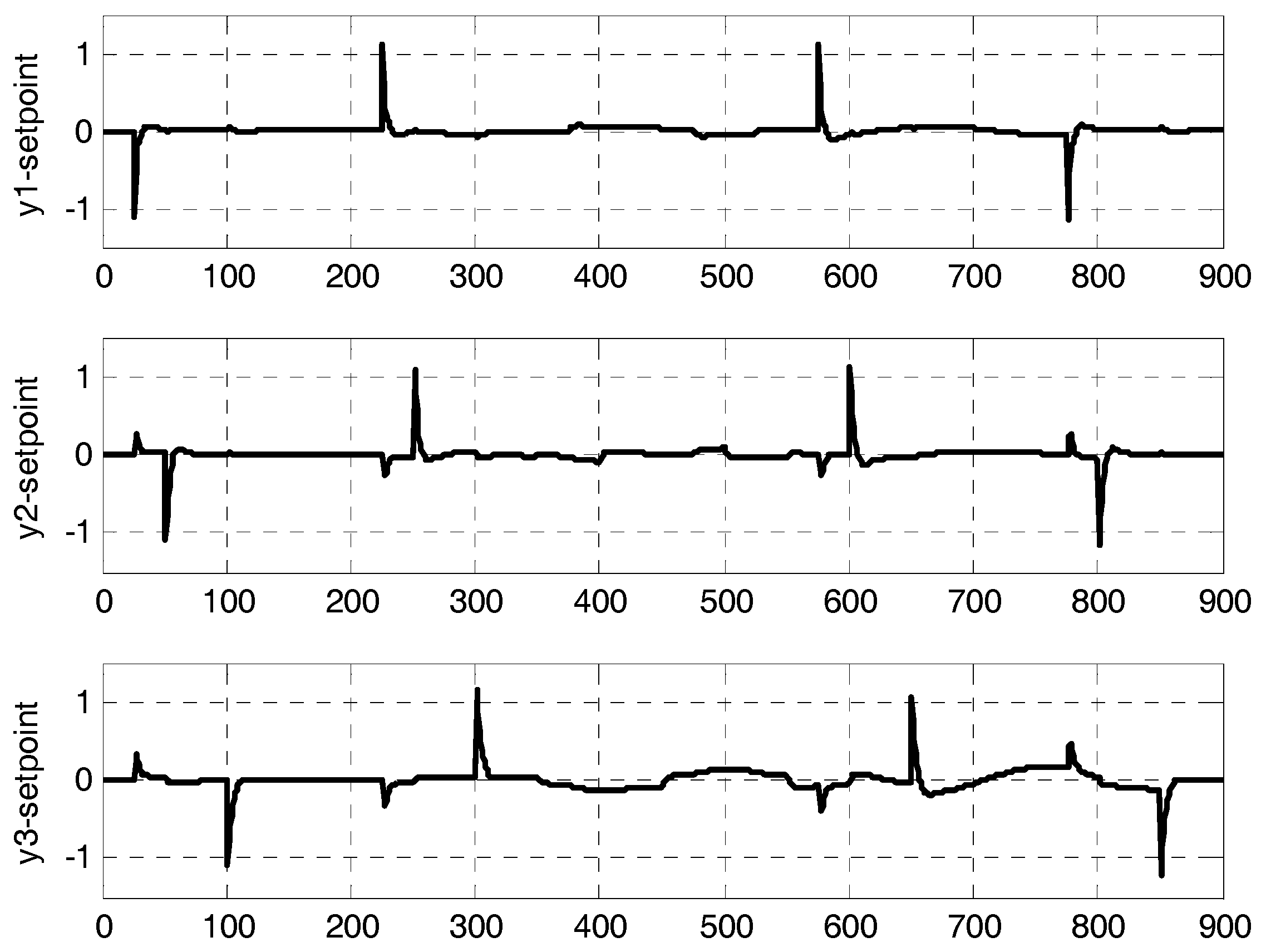
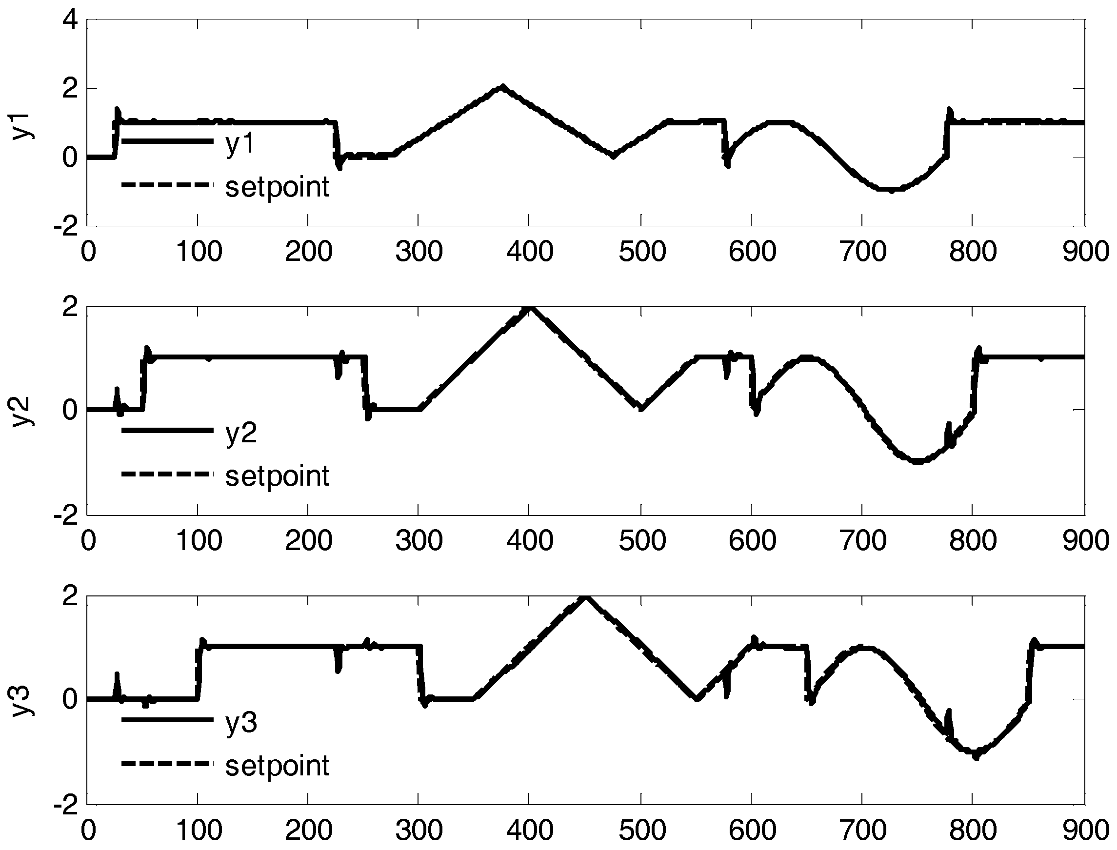
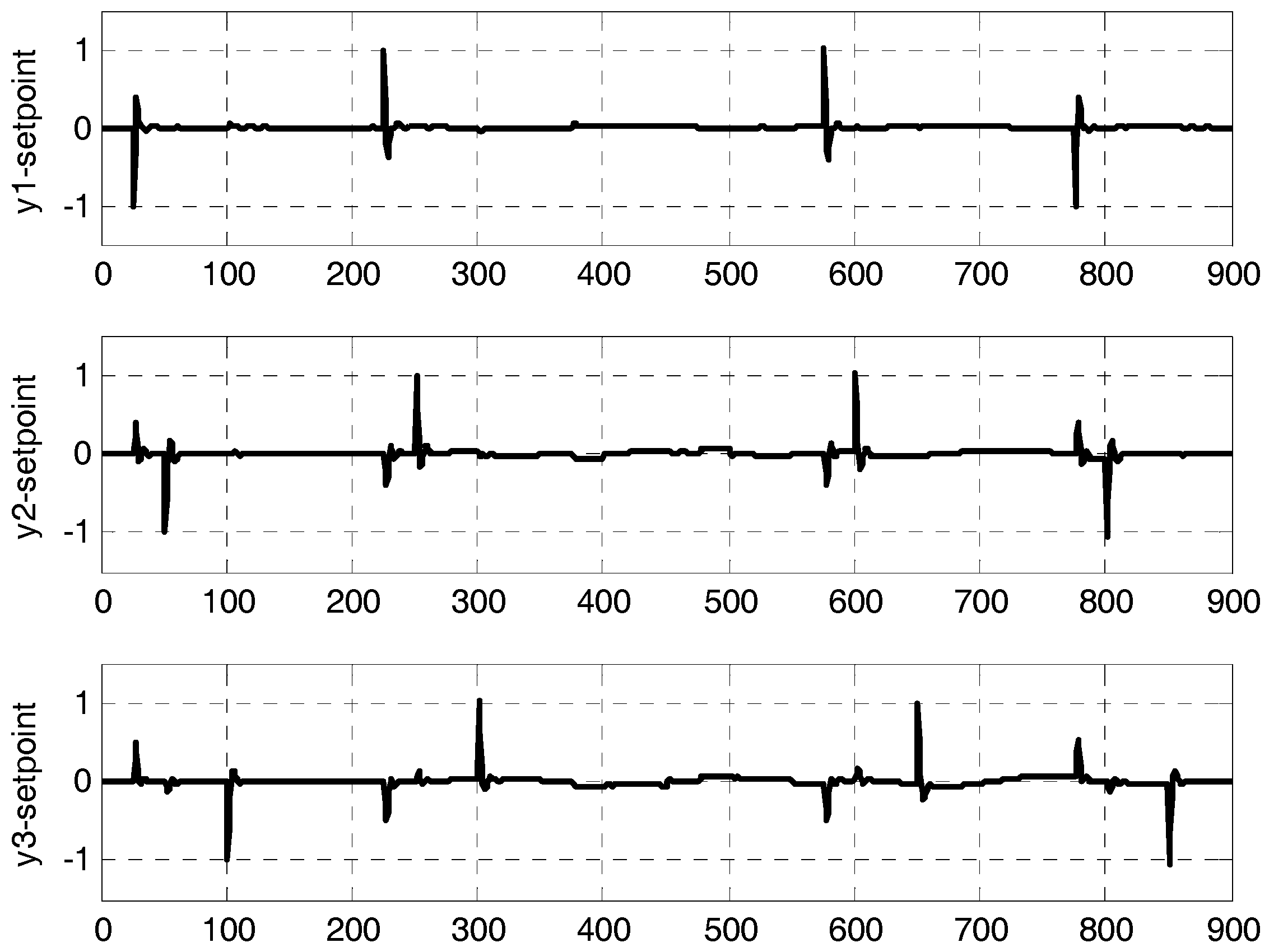
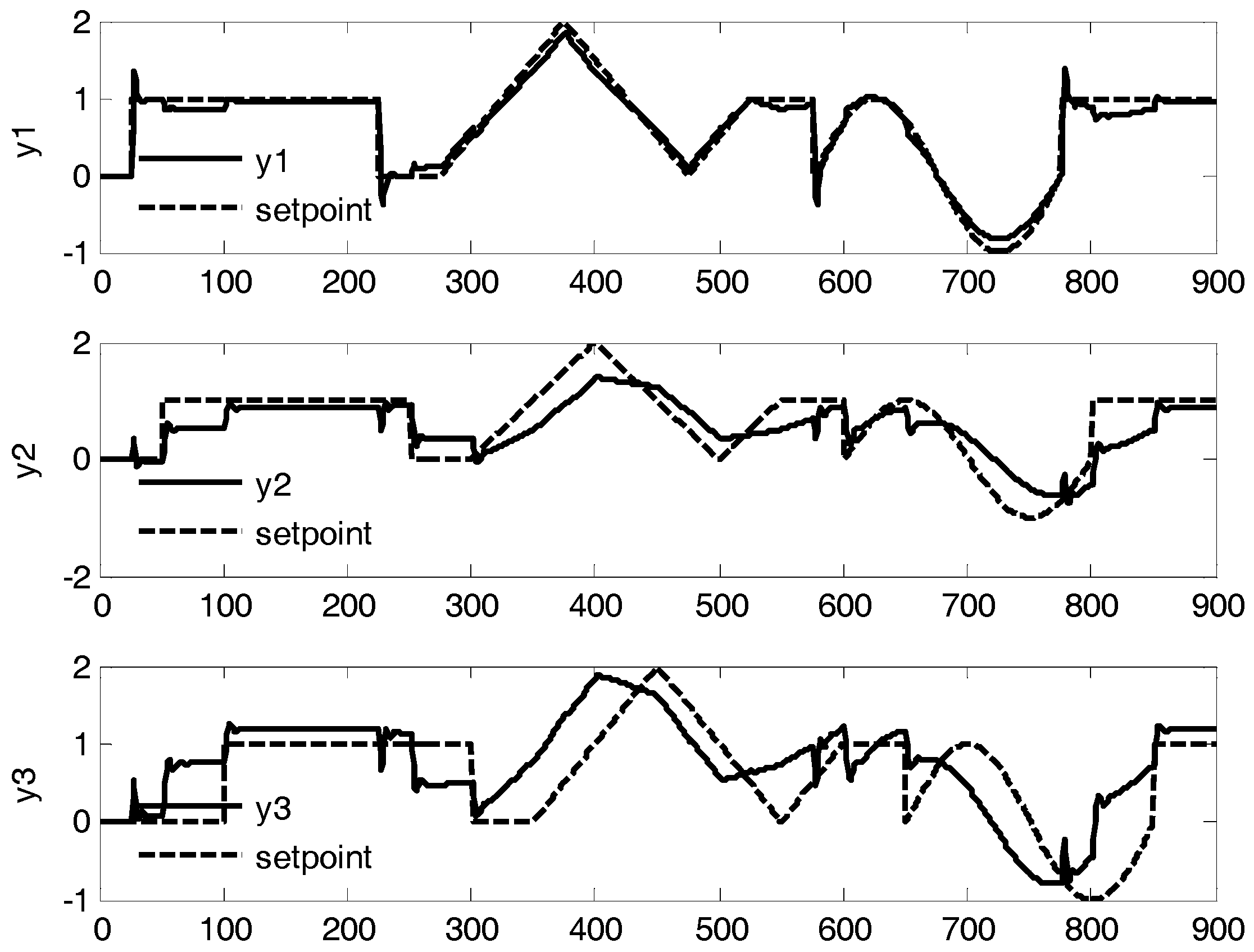
The total simulation horizon for the control comparison is 900. Step signal, ramp signal and sinusoidal signal are used as the set-point of outputs to simulate the common reference signals in industry. In this case study, the conventional MPC, conventional MPC in dynamic PLS and the proposed method are compared together. Control results are shown in Figure 6, Figure 7, Figure 8, Figure 9, Figure 10 and Figure 11. Shown in Figure 7, Figure 9 and Figure 11 are the control error between system outputs and set-points of two methods. In order to evaluate and compare the control performance, the integral of squared error (ISE) between set-points and system outputs is used, results are shown in Table 2. In this case study, Matlab R2012a is used. The configuration of computer is i5 2.6 GHz CPU and 8 GB RAM. Computing time of the three methods are shown in Table 2. From the simulation results, one can conclude that the proposed method has less tracking error than the conventional methods. And the computing time of PLS framework is significantly lower than that of conventional MPC.
Shown in Figure 12 is the control result for third controller is broken. One can see that even if a controller is broken, the proposed method can still keep the system output within a certain range.

5. Conclusions

In this paper, a MPC controller design in the DyPLS framework with an offset-free mechanism was proposed. First, a state space model-based DyPLS model is identified. Based on the obtained model, multiple sub-MPCs are designed. With the integral action in the proposed MPC, offset-free reference tracking performance is guaranteed. With the decoupling character of PLS, the proposed method can be considered as distributed form. It can reduce the calculation burden and is suitable for being embedded into distributed control systems such as network control systems. Furthermore, due to the independently running character of controllers, the proposed method can retain partial control performance for the system when some controllers are broken down.

Acknowledgments

This work was supported by the National Natural Science Foundation of China under Grants 61703191 and supported by Talent Scientific Research Fund of LSHU (No. 00005489).

Author Contributions

Jin Xin proposed the idea and gave formula deduction; Wang Yue wrote this paper; Luo Lin carried out the experiments and analyzed the data; all authors have read and approved the final manuscript.

Conflicts of Interest

The authors declare no conflict of interest.

References

  1. Ge, X.H.; Yang, F.W.; Han, Q.L. Distributed networked control systems: A brief overview. Inf. Sci. 2017, 380, 117–131. [Google Scholar] [CrossRef]
  2. Lyu, L.; Chen, C.L.; Hua, C.Q.; Zhu, S.Y.; Guan, X.P. Co-design of stabilisation and transmission scheduling for wireless control systems. IET Control Theory Appl. 2017, 11, 1767–1778. [Google Scholar] [CrossRef]
  3. Acuna-Bravo, W.; Canuto, E.; Agostani, M.; Bonadei, M. Proportional electro-hydraulic valves: An embedded model control solution. Control Eng. Pract. 2017, 62, 22–35. [Google Scholar] [CrossRef]
  4. Lee, J.H. Model predictive control: Review of the three decades of development. Int. J. Control Autom. Syst. 2011, 9, 415. [Google Scholar] [CrossRef]
  5. Maciejowski, J.M. Predictive Control with Constraints; Prentice-Hall: Upper Saddle River, NJ, USA, 2001. [Google Scholar]
  6. Grüne, L.; Pannek, J. Nonlinear Model Predictive Control; Springer Publishing Company, Incorporated: London, UK, 2013; pp. 2267–2274. [Google Scholar]
  7. Rahmani, M.A.; Alamir, M.; Gualino, D.; Rieu, V. Nonlinear dynamic model identification and mpc control of an organic rankine cycle (orc) based solar thermal power plant. In Proceedings of the 2015 European Control Conference, Linz, Austria, 15–17 July 2015. [Google Scholar]
  8. Ławryńczuk, M. Computationally efficient model predictive control algorithms. Stud. Syst. Decis. Control 2014, 3, 137–149. [Google Scholar]
  9. Lu, Q.; Shi, P.; Lam, H.K.; Zhao, Y. Interval type-2 fuzzy model predictive control of nonlinear networked control systems. IEEE Trans. Fuzzy Syst. 2015, 23, 2317–2328. [Google Scholar] [CrossRef]
  10. Yao, Y.; Gao, F. A survey on multistage/multiphase statistical modeling methods for batch processes. Annu. Rev. Control 2009, 33, 172–183. [Google Scholar] [CrossRef]
  11. Chi, Q.; Fei, Z.; Zhao, Z.; Zhao, L.; Liang, J. A model predictive control approach with relevant identification in dynamic pls framework. Control Eng. Pract. 2014, 22, 181–193. [Google Scholar] [CrossRef]
  12. Kaspar, M.H.; Ray, W.H. Chemometric methods for process monitoring and high-performance controller design. AIChE J. 1992, 38, 1593–1608. [Google Scholar] [CrossRef]
  13. Kaspar, M.H.; Ray, W.H. Dynamic pls modelling for process control. Chem. Eng. Sci. 1993, 48, 3447–3461. [Google Scholar] [CrossRef]
  14. Chen, J.; Cheng, Y.-C.; Yea, Y. Multiloop pid controller design using partial least squares decoupling structure. Korean J. Chem. Eng. 2005, 22, 173–183. [Google Scholar] [CrossRef]
  15. Laurí, D.; Martínez, M.; Salcedo, J.V.; Sanchis, J. Pls-based model predictive control relevant identification: Pls-ph algorithm. Chemom. Intell. Lab. Syst. 2010, 100, 118–126. [Google Scholar] [CrossRef]
  16. Hu, B.; Zheng, P.; Liang, J. Multi-loop internal model controller design based on a dynamic pls framework. Chin. J. Chem. Eng. 2010, 18, 277–285. [Google Scholar] [CrossRef]
  17. Hu, B.; Zhao, Z.; Liang, J. Multi-loop nonlinear internal model controller design under nonlinear dynamic pls framework using arx-neural network model. J. Process Control 2012, 22, 207–217. [Google Scholar] [CrossRef]
  18. LÜ, Y.; Liang, J. Multi-loop constrained iterative model predictive control using arx -pls decoupling structure. Chin. J. Chem. Eng. 2013, 21, 1129–1143. [Google Scholar] [CrossRef]
  19. Huusom, J.K.; Poulsen, N.K.; Jorgensen, S.B.; Jorgensen, J.B. Adaptive disturbance estimation for offset-free siso model predictive control. In Proceedings of the 2011 American Control Conference, San Francisco, CA, USA, 29 June–1 July 2011; IEEE: New York, NY, USA, 2011; pp. 2417–2422. [Google Scholar]
  20. Muske, K.R.; Badgwell, T.A. Disturbance modeling for offset-free linear model predictive control. J. Process Control 2002, 12, 617–632. [Google Scholar] [CrossRef]
  21. Morari, M.; Maeder, U. Nonlinear offset-free model predictive control. Automatica 2012, 48, 2059–2067. [Google Scholar] [CrossRef]
  22. González, A.H.; Adam, E.J.; Marchetti, J.L. Conditions for offset elimination in state space receding horizon controllers: A tutorial analysis. Chem. Eng. Process. Process Intensif. 2008, 47, 2184–2194. [Google Scholar] [CrossRef]
  23. Betti, G.; Farina, M.; Scattolini, R. An mpc algorithm for offset-free tracking of constant reference signals. In Proceedings of the 2012 IEEE 51st Annual Conference on Decision and Control, Maui, HI, USA, 10–13 December 2012; pp. 5182–5187. [Google Scholar]
  24. Betti, G.; Farina, M.; Scattolini, R. A robust mpc algorithm for offset-free tracking of constant reference signals. IEEE Trans. Autom. Control 2013, 58, 2394–2400. [Google Scholar] [CrossRef]
  25. Pannocchia, G.; Gabiccini, M.; Artoni, A. Offset-free mpc explained: Novelties, subtleties, and applications. In Proceedings of the IFAC Conference on Nonlinear Model Predictive Control, Seville, Spain, 17–20 September 2015; pp. 342–351. [Google Scholar]
  26. Borrelli, F.; Morari, M. Offset free model predictive control. In Proceedings of the 46th IEEE Conference on Decision and Control, New Orleans, LA, USA, 12–14 December 2007; pp. 4663–4668. [Google Scholar]
  27. Maeder, U.; Borrelli, F.; Morari, M. Linear offset-free model predictive control. Automatica 2009, 45, 2214–2222. [Google Scholar] [CrossRef]
  28. Pannocchia, G.; Rawlings, J.B. Disturbance models for offset-free model-predictive control. AIChE J. 2003, 49, 426–437. [Google Scholar] [CrossRef]
  29. Maeder, U.; Morari, M. Offset-free reference tracking with model predictive control. Automatica 2010, 46, 1469–1476. [Google Scholar] [CrossRef]
  30. Barker, M.; Rayens, W. Partial least squares for discrimination. J. Chemom. 2003, 17, 166–173. [Google Scholar] [CrossRef]
  31. Wold, S.; Sjostrom, M.; Eriksson, L. Pls-regression: A basic tool of chemometrics. Chemom. Intell. Lab. Syst. 2001, 58, 109–130. [Google Scholar] [CrossRef]
  32. Qin, S.J.; McAvoy, T.J. Nonlinear pls modeling using neural networks. Comput. Chem. Eng. 1992, 16, 379–391. [Google Scholar] [CrossRef]
  33. Lakshminaravanan, S.; Shah, S.L.; Nandakumar, K. Modeling and control of multivariable processes: Dynamic pls approach. AIChE J. 1997, 43, 2307–2322. [Google Scholar] [CrossRef]
  34. Qin, S.J. An overview of subspace identification. Comput. Chem. Eng. 2006, 30, 1502–1513. [Google Scholar] [CrossRef]
  35. Negenborn, R.R.; van Overloop, P.J.; Keviczky, T.; de Schutter, B. Distributed model predictive control of irrigation canals. Netw. Heterog. Media 2009, 4, 359–380. [Google Scholar] [CrossRef]
  36. Embirucu, M.; Fontes, C. Multirate multivariable generalized predictive control and its application to a slurry reactor for ethylene polymerization. Chem. Eng. Sci. 2006, 61, 5754–5767. [Google Scholar] [CrossRef]
Figure 1. Structure of dynamic partial least square (DyPLS) models with state space model.
Information 08 00121 g001
Figure 2. PLS control framework proposed by Kaspar and Ray.
Information 08 00121 g002
Figure 3. The structure of proposed method in distributed form.
Information 08 00121 g003
Figure 4. Input data set for polyethylene reaction.
Information 08 00121 g004
Figure 5. Output data set and modeling results.
Information 08 00121 g005
Figure 6. Control results of conventional model predictive control (MPC) in dynamic PLS.
Information 08 00121 g006
Figure 7. Control error of conventional MPC.
Information 08 00121 g007
Figure 8. Control results of conventional MPC in dynamic PLS.
Information 08 00121 g008
Figure 9. Control error of conventional MPC in dynamic PLS.
Information 08 00121 g009
Figure 10. Control results of offset free MPC in dynamic PLS.
Information 08 00121 g010
Figure 11. Control error of offset free MPC in dynamic PLS.
Information 08 00121 g011
Figure 12. Control results for one controller broken.
Information 08 00121 g012
Table 1. The description of input and output variables.
SymbolDescription
inputx1monomer feed flow
x2solvent(n-hexane) feed flow
x3catalyst feed flow
x4gas recycle/monomer feed ratio
outputy1production
y2slurry polymer
y3catalyst efficiency
Table 2. Integral of squared error (ISE) and computing time of three methods.
Conventional MPCConventional MPC in Dynamic PLSProposed Method
ISE of y137.336.385.70
ISE of y252.219.267.80
ISE of y331.9814.739.08
Computing time (ms)87.2363.8764.37