Article

A Novel Grey Prediction Model Combining Markov Chain with Functional-Link Net and Its Application to Foreign Tourist Forecasting

1
College of Management & College of Tourism, Fujian Agriculture and Forestry University, Fuzhou 350002, China
2
Department of Business Administration, Chung Yuan Christian University, Taoyuan 32023, Taiwan
3
School of Economics and Management, Dalian Ocean University, Dalian 116023, China
4
Department of Business Management, National Taipei University of Technology, Taipei 10608, Taiwan
*
Author to whom correspondence should be addressed.
Information 2017, 8(4), 126; https://doi.org/10.3390/info8040126
Submission received: 31 August 2017 / Revised: 29 September 2017 / Accepted: 3 October 2017 / Published: 13 October 2017
(This article belongs to the Section Information Systems)

Abstract

:
Grey prediction models for time series have been widely applied to demand forecasting because only limited data are required for them to build a time series model without any statistical assumptions. Previous studies have demonstrated that the combination of grey prediction with neural networks helps grey prediction perform better. Some methods have been presented to improve the prediction accuracy of the popular GM(1,1) model by using the Markov chain to estimate the residual needed to modify a predicted value. Compared to the previous Grey-Markov models, this study contributes to apply the functional-link net to estimate the degree to which a predicted value obtained from the GM(1,1) model can be adjusted. Furthermore, the troublesome number of states and their bounds that are not easily specified in Markov chain have been determined by a genetic algorithm. To verify prediction performance, the proposed grey prediction model was applied to an important grey system problem—foreign tourist forecasting. Experimental results show that the proposed model provides satisfactory results compared to the other Grey-Markov models considered.

1. Introduction

Both time series and econometric methods have been commonly used for demand forecasting. However, prediction performance of econometric methods can be significantly influenced by incomplete information associated with explanatory factors; and models for time series, such as ARIMA [1] and Box-Jenkins models, usually require large size of samples to obtain reasonable prediction accuracy [2,3,4,5]. Neural networks, such as multilayer perceptron and support vector regression, have also been applied to demand forecasting [6,7]. Although the neural network has proven to be an efficient technique involving computational intelligence in representing complex nonlinear mappings, similar to econometric methods, multilayer perceptron and support vector regression suffer from incomplete information associated with input variables.
Grey prediction models [8] have the ability to characterize an unknown system with small data sets [9], without requiring conformance to statistical assumptions such as normality distribution. For time series prediction, GM(1,1) is among the most frequently used grey prediction models [10]. It requires only four recent samples to derive reliable and acceptable prediction accuracy [5], and has been widely applied to various decision problems involving management, economics, and engineering [2,3,4,11,12,13,14,15,16]. To better improve the prediction performance of the original GM(1,1) model, several versions combining with computational intelligence have been proposed, such as models with self-adaptive intelligence [17], neural-network-based grey prediction for electricity consumption prediction [18,19], PGM(1,1) using particle swarm optimization to determine the development coefficient [20], GM(1,1) models with online sequential extreme learning machine [21], an optimized nonlinear grey Bernoulli model [22], an adaptive GM(1,1) for electricity consumption [3], and grey wave forecasting through qualified contour sequences [23]. Literally, the combination of grey prediction and neural networks can better represent system dynamics with uncertainty and nonlinearity [21].
The GM(1,1) model with residual modification could be established to improve prediction accuracy of the original GM(1,1) model [7,9]. To modify the predicted values from the original model, a residual modification model is commonly set up by building the original GM(1,1) model, and then constructing the residual GM(1,1) model by a residual series [4,19]. As a matter of facts, construction of grey prediction models with residual modification all stemmed from the foundation of the GM(1,1) residual model. It is interesting that prediction accuracy obtained by the original GM(1,1) model can be effectively improved using the Markov chain to realize the residual model [24,25]. The Grey-Markov model, MCGM(1,1) uses the GM(1,1) model to get the basic trend of the original data, and then uses the Markov chain to fix residual errors generated by the GM(1,1) model. It has shown advantages over the GM(1,1) model, when the time series data fluctuated significantly [26,27]. Other related MCGM(1,1) studies, such as Hsu and Wen [28] and Hsu [29] used Markov chain sign estimation to modify residuals for the trans-Pacific air passenger market and the global integrated circuit industry. Hsu et al. [30] combined a Fourier grey model with Markov chain to predict turning time of the stock market. Kumar and Jain [31] applied MCGM(1,1) to predict conventional energy consumption. Li et al. [32] combined RGM(1,1) with the Markov chain for thermal electric power generation. Mao and Sun [33] applied MCGM(1,1) to fire accident prediction. Sun et al. [25] proposed a MCGM(1,1) variant using the Cuckoo search algorithm for foreign tourist arrivals prediction. Wang [34] showed the effectiveness of MCGM(1,1) for tourism demand prediction. Xie et al. [35] proposed a QP-Markov model to estimate the probability that one energy component can transit to another energy component.
However, for an MCGM(1,1)-based model, it is not easy to determine the number of states and their bounds for the Markov chain—these parameters are usually specified in advance through experience and the modification range for a predicted value derived by the original GM(1,1) model is identical to its corresponding predicted residual from the Markov chain. These more or less have an impact on prediction performance. Because of the advantage of combining grey prediction with neural networks, we propose a residual modification model based on neural networks, NN-Grey-Markov, incorporating a functional link net (FLN) with effective function approximation capability [36,37,38,39] to estimate the modification range with respect to a predicted residual obtained from the Markov chain. The genetic algorithm (GA) is employed to determine connection weights of an FLN, the number of states, and the bounds of each state, to construct the proposed grey prediction model with high prediction accuracy.
Foreign tourist forecasting can be recognized to be a grey system problem since several factors influence tourism demand in uncertain ways. That is, several factors such as exchange rate, security, and disease cause fluctuations in tourism demand but the precise manner of this effect is not clear. The variety of the international tourism market has meant foreign tourist prediction has been a challenging task for tourism administrators [25,40,41]. The global tourism industry has a significant impact on a nation’s economic development and foreign tourist forecasting plays a very important role when devising tourism development plans for cities or countries. It therefore makes us more intrigued to examine the prediction performance of the proposed residual modification model on foreign tourist forecasting.
The remainder of the paper is organized as follows: Section 2 introduces the MCGM(1,1) model and Section 3 presents the proposed NN-Grey-Markov model. Section 4 validates the prediction accuracy of the proposed grey prediction model for foreign tourist forecasting using two real cases. This paper is concluded with Section 5.

2. The MCGM(1,1) Model

2.1. Original GM(1,1) Model

By one time accumulated generating operation (1-AGO) [9], a new sequence, x ( 1 ) = ( x 1 ( 1 ) , x 2 ( 1 ) , …, x n ( 1 ) ), can be generated from an original data sequence x ( 0 ) = ( x 1 ( 0 ) , x 2 ( 0 ) , …, x n ( 0 ) ) as follows:
x k ( 1 ) = j = 1 k x k ( 0 ) , k =   1 ,   2 ,   , n
and x 1 ( 1 ) , x 2 ( 1 ) , …, x n ( 1 ) can be approximated by a first-order whitenization differential equation,
d x ( 1 ) d t   + a   x ( 1 ) =   b
where a is the developing coefficient and b is the control variable. Using 1-AGO is beneficial to identify regularity hidden in data sequences, even if the original data are finite, insufficient, and chaotic.
The predicted value, x ^ k ( 1 ) , for x k ( 1 ) can be obtained by solving the differential equation with initial condition x 1 ( 1 ) = x 1 ( 0 ) ,
x ^ k ( 1 ) = ( x 1 ( 0 ) b a ) e a ( k 1 ) + b a
Thus, x ^ 1 ( 1 ) = x 1 ( 0 ) holds, and a and b can be estimated from the grey difference equation
x k ( 0 ) + a z k ( 1 ) = b
where z k ( 1 ) is the background value,
z k ( 1 ) = α x k ( 1 ) + ( 1   α ) x k 1 ( 1 )
where α = 0.5 usually, for convenience. Using n − 1 grey difference equations (k = 2, 3, …, n), a and b can be derived using the ordinary least squares approach,
[a, b]T = (BTB)1BTy
where
B = [ z 2 ( 1 ) 1 z 3 ( 1 ) 1 z n ( 1 ) 1 ]
and
y = [ x 2 ( 0 ) , x 3 ( 0 ) , , x n ( 0 ) ] T
Using the inverse AGO, the predicted value of x k ( 0 ) is
x ^ k ( 0 ) = x ^ k ( 1 ) x ^ k 1 ( 1 ) , k =   2 ,   3 ,   , n
Therefore,
x ^ k ( 0 )   =   ( 1 e a )   ( x 1 ( 0 ) b a ) e a ( k 1 ) , k =   2 ,   3 ,   , n
and x ^ 1 ( 1 ) = x ^ 1 ( 0 ) holds.

2.2. Residual Modification by Markov Chain

Let ε = ( ε 1 , ε 2 , …, ε n ) denote the sequence of residual values, where
ε k = | x k ( 0 ) x ^ k ( 0 ) | , k =   1 ,   2 ,   , n
Let [ ε min , ε max ] denote the range of residuals, where ε min and ε max are the minimum and maximum values among ε k , respectively. Then [ ε min , ε max ] can be divided into r intervals (r ≥ 2), with each interval treated as a state. The state with lower bound ε min is state 1, and state r is the state with upper bound ε max . Therefore, state of ε k can be determined depending on where it locates. It is not necessary to require intervals with equal length.
Subsequently, an m-step transition probability matrix P(m) can be generated as follows:
P ( m ) = [ p 11 ( m ) p 12 ( m ) p 1 r ( m ) p 21 ( m ) p 22 ( m ) p 2 r ( m ) p r 1 ( m ) p r 2 ( m ) p r r ( m ) ]
where p i j ( m ) denotes the transition probability from state i to j (1 ≤ i, jr) by m steps,
p i j ( m ) = t i j ( m ) t i
where t i j ( m ) denotes the number of transitions from state i to j by m steps, and ti denotes the number of state i among the sequence of residual values. For each row in P(m), the sum of elements equals one. However, p i i ( m ) can be specified directly as one when the sum of elements in the row i equals zero. In other words, such a state is treated as an absorbing state.
The predicted residual value, ε ^ k ( m ) can be computed if ε k locates in state i,
ε ^ k ( m ) = p i 1 ( m ) c 1 + p i 2 ( m ) c 2 + + p i r ( m ) c r
where cw (1 ≤ wr) is the center of state w, whose lower and upper bounds are lw and uw, respectively. Alternatively, cw can be expressed as [25,32]
cw = αw lw + (1 − αw) uw
Then x ^ k ( 0 ) can be revised as a new predicted value x ˜ k ( 0 ) by adding the predicted residual ε ^ k ( m ) .
x ˜ k ( 0 ) = x ^ k ( 0 ) + ε ^ k ( m ) , k =   1 ,   2 ,   , n
The Markov chain is used to modify the residuals generated by the GM(1,1) model. Sun et al. [25] and Mao and Sun [33] used the sequence of relative errors rather than the sequence of residual values.

3. The Proposed NN-Grey-Markov Model

Two issues must be addressed for the original Grey-Markov model. First, the modification range of x ^ k ( 0 ) in the original Grey-Markov model is restricted to ε ^ k ( m ) with a positive sign, which may affect prediction accuracy of the residual modification models. To increase flexibility, the restriction may be relaxed by deriving the sign and modification range with respect to ε ^ k ( m ) . Second, the number of intervals, r, is fixed and usually specified in advance. To improve prediction accuracy it is reasonable to apply a GA—which is a powerful search and optimization method [42,43,44]—to automatically determine r and the lower and upper bounds of each interval. FLN is an appropriate tool to provide estimations for the sign and modification range, due to its effective function approximation capability.
Section 3.1 describes how to apply FLN to estimate the sign and modification range for each predicted residual, and Section 3.2 describes the construction of the proposed NN-Grey-Markov model using GA to determine the required parameters, including FLN connection weights, r and the lower and upper bounds of each interval.

3.1. Incorporating Functional-Link Net into the Proposed NN-Grey-Markov Model

For flexibility, it is reasonable to modify x ^ k ( 0 ) as x ˜ k ( 0 ) by adding or subtracting ε ^ k ( m ) ,
x ˜ k ( 0 ) = x ^ k ( 0 ) + y k ε ^ k ( m ) , k =   1 ,   2 ,   , n
where yk ranges from −1 to 1 and can be interpreted as the degree to which x ^ k ( 0 ) can be adjusted. That is, if yk is positive, the greater yk, the more likely x ^ k ( 0 ) is to be adjusted toward x ^ k ( 0 ) + ε ^ k ( m ) . On the contrary, if yk is negative, the smaller yk, the more likely x ^ k ( 0 ) is to be adjusted toward x ^ k ( 0 ) ε ^ k ( m ) . We estimated yk with FLN using the hyperbolic tangent function,
tanh ( z )   = e z e z e z + e z
as the activation function, which has range (−1, 1).
An enhanced pattern with respect to a single input denoted by tk, can be generated as (tk, sin(πtk), cos(πtk), sin(2πtk), cos(2πtk), sin(4πtk)) through a functional link, where tk denotes the time period k with respect to x ^ k ( 0 ) . Let θ be the bias to the output node. Then the actual output value, yk, corresponding to (tk, sin(πtk), cos(πtk), sin(2πtk), cos(2πtk), sin(4πtk)) is
yk = tanh(w1tk + w2sin(πtk) + w3cos(πtk) + w4sin(2πtk) + w5cos(2πtk) + w6sin(4πtk) + θ)
Although the components in the functional expansion representation can be unrestrictedly extended for tk, this is not practical in real applications. (tk, sin(πtk), cos(πtk), sin(2πtk), cos(2πtk), sin(4πtk)) with respect to tk is acceptable [37]. Hu [45] also demonstrated the superiority of applying residual modification using FLN to predict energy demand.

3.2. Constructing the Proposed NN-Grey-Markov Model

To construct the proposed grey prediction model with high prediction accuracy, we consider the mean absolute percentage error (MAPE), which is usually recommended to be used for modelling [46,47]. MAPE with respect to x ( 0 ) is formulated as follows:
MAPE = 1 n k = 1 n | x k ( 0 ) x ˜ k ( 0 ) | x k ( 0 ) × 100 %
What we are aiming for is to set up a prediction model with high prediction accuracy. The problem can be formulated as maximizing the reciprocal of MAPE for constructing the prediction model. Using this fitness function, a real-valued GA was developed to automatically determine 7 + 2r parameters, including the connection weights (w1, w2, w3, w4, w5, w6), bias (θ), the number of intervals (r), partition points (p1, p2, …, pr−1), and relative weights in respective intervals (α1, α2, …, αr) for the proposed grey prediction model, where w1, w2, w3, w4, w5, w6, and θ range from −1 to 1, p1, p2, …, pr−1 range from ε min to ε max , and r range from 2 to 10. It is noted that ur−1 = lr = pr−1 holds.
Let nsize and nmax denote the population size and maximum number of generations, respectively, and Pm denote the population in generation m (1 ≤ mnmax). After evaluating the fitness value of each chromosome in Pm, nsize new chromosomes were generated for Pm+1 by means of selection, crossover, and mutation. GA was performed for nmax generations. When the stopping condition was satisfied, the algorithm is terminated, and the best chromosome with maximum fitness value among consecutive generations can be used to examine the generalization ability of the NN-Grey-Markov model. These genetic operations are briefly described below.

3.2.1. Selection

Let chromosome u (1 ≤ unsize) produced in Pm be represented as w u , 1 m w u , 2 m w u , 3 m w u , 4 m w u , 5 m w u , 6 m θ u m r u m p u , 1 m p u , 2 m p u , r 1 m α u , 1 m α u , 2 m α u , r m . Two chromosomes from Pm were randomly selected by binary tournament selection, and the one with higher fitness was put into a mating pool. This process was repeated until nsize chromosomes were placed in the mating pool. nsize/2 pairs of chromosomes from the pool were then randomly selected, and offspring of the selected parents were reproduced by crossover and mutation.

3.2.2. Crossover

Crossover was applied to reproduce children by altering the parent chromosomal makeup. For two selected chromosomes, u ( w u , 1 m w u , 2 m w u , 3 m w u , 4 m w u , 5 m w u , 6 m θ u m r u m p u , 1 m p u , 2 m p u , r 1 m α u , 1 m α u , 2 m α u , r m ) and v ( w v , 1 m w v , 2 m w v , 3 m w v , 4 m w v , 5 m w v , 6 m θ v m r v m p v , 1 m p v , 2 m p v , r 1 m α v , 1 m α v , 2 m α v , r m ) (1 ≤ vnsize), each pair of real-valued genes can be used to generate two new genes with crossover probability Prc.
w u , i m   =   h i w u , i m   +   ( 1     h i ) w v , i m ,   w v , i m   =   ( 1     h i ) w u , i m   +   h i w v , i m ,   i   =   1 ,   2 ,   ,   6 θ u m   =   h 7 θ u m   +   ( 1     h 7 ) θ v m ,   θ v m   =   ( 1     h 7 )   θ u m   +   h 7 θ v m r u m   =   h 8 r u m   +   ( 1     h 8 ) r v m ,   r v m =   ( 1     h 8 )   r u m   +   h 8 r v m p u , i m   =   h 8 + j p u , i m   +   ( 1     h 8 + j ) p v , i m ,   p v , i m   =   ( 1     h 8 + j ) p u , i m   +   h 8 + j p v , i m ,   j   =   1 ,   2 ,   ,   r     1 α u , i m   =   h 7 + r + j α u , i m   +   ( 1     h 7 + r + j ) α v , i m ,   p v , i m   =   ( 1     h 7 + r + j ) α u , i m   +   h 7 + r + j α v , i m ,   j   =   1 ,   2 ,   ,   r
where h1, h2, , h7+2r are all random numbers in the interval [0, 1]. It is noted that Prc should be specified as a large value because it controls the exploratory range in the solution space.

3.2.3. Mutation

Mutation was performed with probability Prm for each real valued parameter in a new chromosome generated by crossover. To avoid excessive perturbation, a low mutation rate was taken into account. When a mutation happened with a real valued gene, that gene was changed by adding a randomly selected number from a specified interval. After crossover and mutation, ndel (0 ≤ ndelnsize) chromosomes in Pm+1 were removed randomly from the set of new chromosomes to create space for the chromosome with maximum fitness value in Pm.

4. Empirical Study

4.1. Background

The global tourism industry plays a significant role in the economic development of a country. To boost the tourism industry, devising tourism development and marketing strategies by estimating the number of the foreign tourists has become increasingly important for governments and industries in the private sector such as airlines, hospitality services, and travel agencies. Effective tourism demand forecasting can significantly affect the amount of resources that governments and private sectors invest [6]. In Taiwan, tourism statistics show that foreign tourists mainly came from Japan, Hong Kong, Macao, Korea, China, and USA for 2014–2016. It is noteworthy that the number of tourist arrivals from Southeast Asia increased by 15% in May 2016 compared to May 2015. In face of the growth rate, authorities have actively investigated how to continuously expand the tourism market in the Southeast Asia through new policies. Therefore, foreign tourist forecasting will have a great impact on the outcomes of programs related to the policy.
Real datasets are used to conduct experiments to compare foreign tourist forecasting from the proposed NN-Grey-Markov model against the original GM(1,1), MCGM(1,1), and several models proposed by Sun et al. [25], including segmented GM(1,1) (SGM(1,1)), SGM(1,1) using Markov chain (MCSGM(1,1)), and MCSGM(1,1) using a Cuckoo search algorithm (CMCSGM(1,1)). In contrast to the original GM(1,1) and MCGM(1,1) using all observed data, the SGM model first used a rolling mechanism to determine the set of newly observed data, and then constructed the GM(1,1) model. Thus, the rolling mechanism could select only a few recent data by capturing the developing trend from all observed data. This reflects the premise that as the system develops, the significance of older data reduces [9].
As the system develops further, the significance of the older data reduces [9,48]. Therefore, the training data, retained after rolling, were applied to the SGM(1,1), MCSGM(1,1) and CMCSGM(1,1) models. The rolling mechanism could select only a few recent data by capturing the developing trend from the training data. For x ( 0 ) = ( x 1 ( 0 ) , x 2 ( 0 ) , …, x n ( 0 ) ), the l-point rolling (4 ≤ ln − 1) can be exercised on x ( 0 ) to construct a GM(1,1) model. MAPEl corresponding to the l-point rolling can be computed as
MAPE l = 1 n l k = l + 1 n | x k ( 0 ) x ˜ k ( 0 ) | x k ( 0 ) × 100 %
Finally, the best number of point, say v, that can be used to construct a GM(1,1) model, called SGM(1,1), is determined as
v = arg min l MAPE l
For fair comparisons, the proposed NN-Grey-Markov model used the same training data as the SGM(1,1), the MCSGM(1,1), and the CMCSGM(1,1) models. The rest of this section is organized as follows. Section 4.1 presents the parameter specifications for the GA and Section 4.2 presents prediction accuracy for different grey prediction models on real data.

4.2. GA Parameters

It is known that population size and crossover and mutation probabilities can have impacts on GA performance. There are no optimal parameter settings. Therefore, following [42,44], the experiment parameters were chosen to be:
(i)
nsize = 200: It is reasonable to specify population size ranging from 50 to 500 individuals.
(ii)
nmax = 1000: nmax plays a role of stopping condition, and it should take available computing time into account.
(iii)
ndel = 2: A small number of elite chromosomes is considered.
(iv)
Prc = 0.8, Prm = 0.01.
In the experiment, no matter what the data set is, the same parameters of GA were used to examine the prediction accuracy of the proposed NN-Grey-Markov model.

4.3. Applications to Foreign Tourist Forecasting

4.3.1. Case I

The first experiment was conducted on the yearly statistics reported by Taiwan Tourism Bureau [49]. Table 1 shows historical annual foreign tourists to Taiwan from six countries, Japan, Hong Kong/Macao, Korea, China, USA, and Southeast Asia, collected from 2001 to 2016. Year 2016 was used for testing using a one-step transition probability matrix, i.e., m = 1. Therefore, after performing the rolling mechanism, 2011–2015 data from China and 2012–2015 from the other countries can be used for model-fitting for the SGM(1,1), the MCSGM(1,1), the CMCSGM(1,1), and proposed grey prediction models. Whichever the country is, the original GM(1,1) and the MCGM(1,1) were constructed using data from 2001 to 2015.
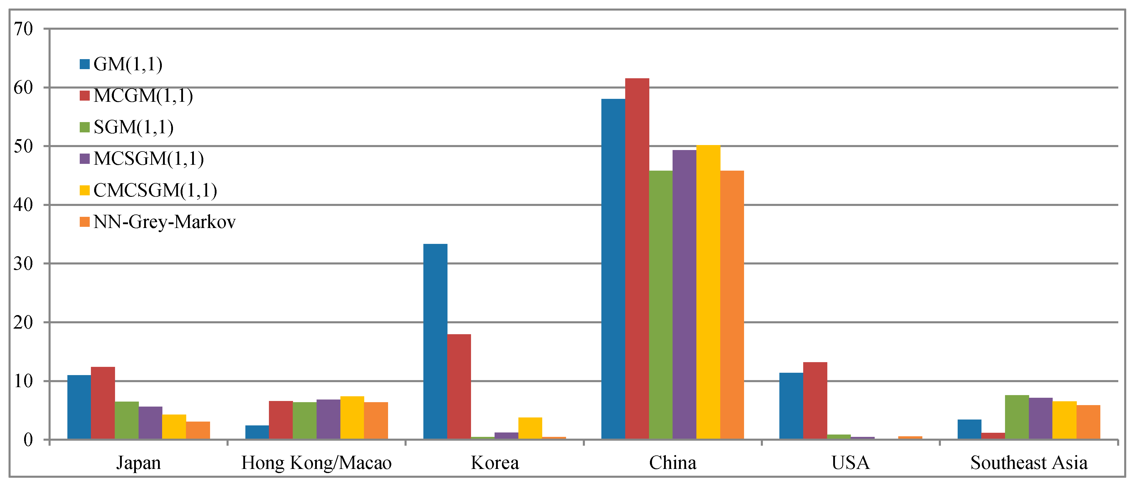
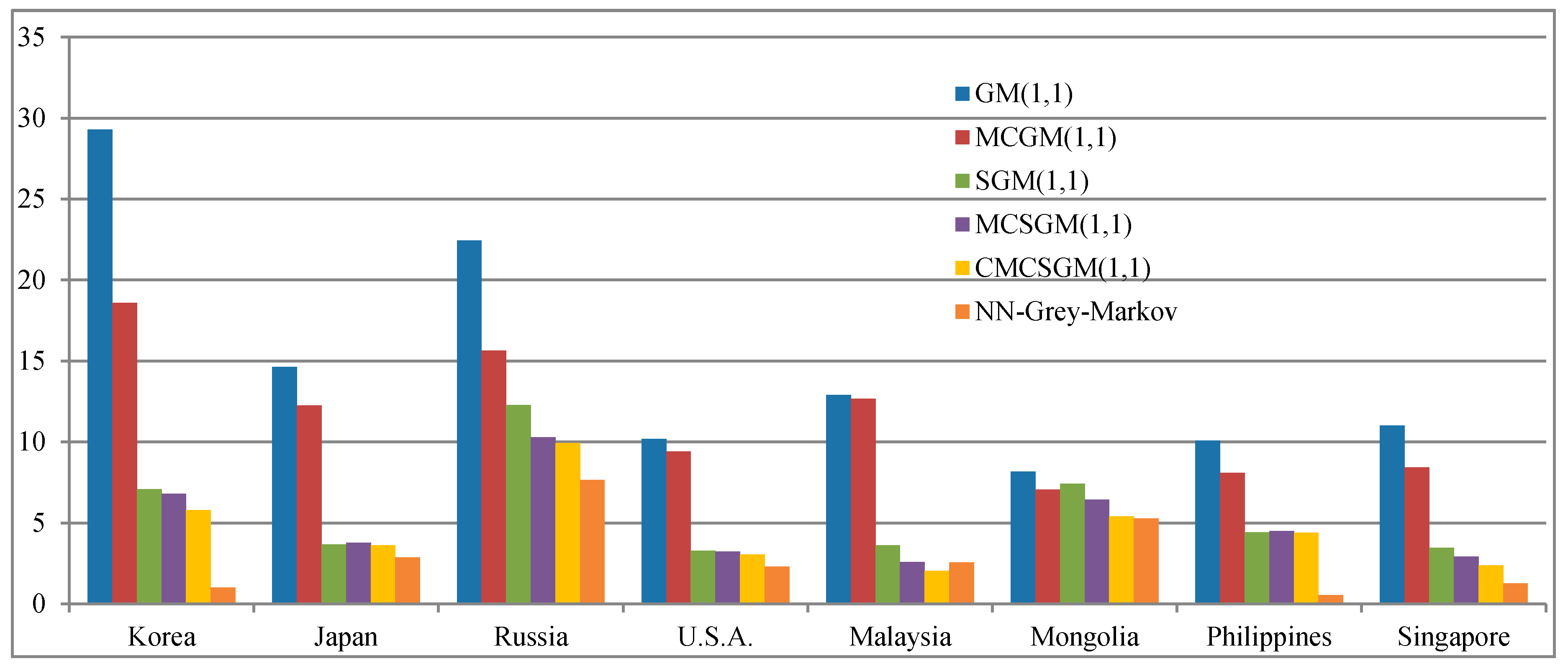
Figure 1 and Figure 2 show prediction results with respect to model fitting and testing for different models, respectively. Figure 1 shows that the proposed NN-Grey-Markov model outperforms the other prediction models considered for model-fitting. For testing, the proposed NN-Grey-Markov model outperforms the SGM(1,1), the MCSGM(1,1), and the CMCSGM(1,1) models, and it is little inferior to the original GM(1,1) and the MCGM(1,1) models for Hong Kong/Macao and Southeast Asia.

4.3.2. Case II

Historical annual data from 1997 to 2013 published by China National Tourism Administration were used to conduct the second experiment. The data were summarized in Reference [25]. The collected data were associated with foreign tourists from eight main countries, including Japan, Korea, Malaysia, Mongolia, Philippines, Russia, Singapore, and USA. Year 2013 was used for testing by a one-step transition probability matrix. Performing the rolling mechanism, 2005–2012 data from Korea, Japan, USA, and Malaysia; 2006–2012 from Russia, 2003–2012 from Mongolia and Philippines; and 2004–2012 from Singapore from 2004 to 2012 can be used to construct the SGM(1,1), the MCSGM(1,1), the CMCSGM(1,1), and proposed NN-Grey-Markov models. The original GM(1,1) and the MCGM(1,1) were constructed using data from 1997 to 2012 for each economy. Using the same data, Sun et al. [25] demonstrated the effectiveness of the CMCSGM(1,1) model.
Figure 3 and Figure 4 show prediction results with respect to model fitting and testing for different prediction models, respectively. For model-fitting, Figure 3 shows that the proposed NN-Grey-Markov model is comparable or superior to the compared models. It is slightly inferior to the CMCSGM(1,1) model for Malaysia. As for testing results, prediction accuracy of the proposed NN-Grey-Markov model outperforms that of the CMCSGM(1,1) model, except for Malaysia and Singapore. The proposed grey prediction model is superior to the original GM(1,1), the SGM(1,1), and the MCSGM(1,1) models. It is obvious that the proposed NN-Grey-Markov model provides comparable and satisfactory results compared to the other prediction models considered.

5. Discussion and Conclusions

Data fluctuations such as tourism time series data often arise from random factors, which can be effectively reduced by the Grey-Markov model. Based on the Grey-Markov model, this study proposed a novel grey residual modification model, NN-Grey-Markov, for tourism demand prediction. Compared to previous studies based on MCGM(1,1), there are two distinctive features of the proposed NN-Grey-Markov model. First, the proposed grey prediction model incorporates FLN to estimate the sign of each revised residual, and available degree to which a predicted value from the GM(1,1) model can be adjusted. Second, we need not define the number of states and their bounds for the Markov chain in advance, since these can be fully determined by GA. It should be noted that, the FLNGM(1,1) model [45] integrated the original GM(1,1) with the residual GM(1,1) models and then used the functional-link net to estimate the sign and the modification range with respect to a predicted residual obtained from the residual GM(1,1) model. The implementation of the proposed NN-Grey-Markov model is therefore different from that of the FLNGM(1,1) model.
Development of the tourism industry has contributed relatively highly to economic prosperity. In the variable global tourism market, accurate prediction of tourism demand is crucial for governments and private sectors to set up strategies—such as investment and construction—to promote the tourism industry. It is challenging to predict precisely the trend of tourism demand. From the perspective of the grey system, it is reasonable to apply the GM(1,1) model to foreign tourist prediction. Historical annual data for foreign tourists, collected from Taiwan and China official institutions, were used to evaluate prediction performance of the proposed NN-Grey-Markov model. The proposed model with pre-specified GA parameters, including population size, number of generations, probabilities for crossover and mutation, performs well. This means that fine parameter tuning is not required for the proposed prediction model, and that parameter specifications introduced in the previous section were acceptable. Real case experiments reveal that the proposed NN-Grey-Markov model outperformed other grey prediction models considered for the majority of data sets. This validated the potential usefulness of the proposed NN-Grey-Markov model for tourism demand prediction.
For future studies, there are two issues that require addressing. First, this study used a one-step transition probability matrix to predict the residual for testing on a predicted time period. The other alternative is to sum the rows of the transition probability matrices corresponding to some near time periods prior to a predicted one to estimate the residual corresponding to a predicted time period [32,33]. It would be interesting to examine the influence on foreign tourist prediction using the proposed NN-Grey-Markov model. Second, FLN used the hyperbolic tangent function as the output neuron’s activation function, computing a weighted sum of a vector of connection weights with an enhanced pattern. This assumes additivity among individual variables in the enhanced pattern [50]. However, these criteria are not always independent [12,51,52], and would be interesting to explore the impact of non-additivity on prediction performance of the proposed NN-Grey-Markov model.

Acknowledgments

The authors would like to thank the anonymous referees for their valuable comments. This research is supported by the Ministry of Science and Technology, Taiwan under grant MOST 106-2410-H-033-006-MY2.

Author Contributions

Yi-Chung Hu conceived the research; Yi-Chung Hu and Peng Jiang performed the experiments; Yu-Jing Chiu collected and analyzed data; Yi-Chung Hu, Peng Jiang, and Jung-Fa Tsai wrote the paper; and Yu-Jing Chiu revised the paper. All authors have read and approved the final version.

Conflicts of Interest

The authors declare no conflict of interest.

References

  1. Ediger, V.S.; Akar, S. ARIMA forecasting of primary energy demand by fuel in Turkey. Energy Policy 2007, 35, 1701–1708. [Google Scholar] [CrossRef]
  2. Feng, S.J.; Ma, Y.D.; Song, Z.L.; Ying, J. Forecasting the energy consumption of China by the grey prediction model. Energy Sour. B Econ. Plan. Policy 2012, 7, 376–389. [Google Scholar]
  3. Li, D.C.; Chang, C.J.; Chen, C.C.; Chen, W.C. Forecasting short-term electricity consumption using the adaptive grey-based approach-An Asian case. Omega 2012, 40, 767–773. [Google Scholar] [CrossRef]
  4. Pi, D.; Liu, J.; Qin, X. A grey prediction approach to forecasting energy demand in China. Energy Sour. A Recovery Util. Environ. Eff. 2010, 32, 1517–1528. [Google Scholar] [CrossRef]
  5. Wang, C.H.; Hsu, L.C. Using genetic algorithms grey theory to forecast high technology industrial output. Appl. Math. Comput. 2008, 195, 256–263. [Google Scholar] [CrossRef]
  6. Cankurt, S.; Subasi, A. Developing tourism demand forecasting models using machine learning techniques with trend, seasonal, and cyclic components. Balkan J. Electr. Comput. Eng. 2015, 3, 42–49. [Google Scholar]
  7. Lin, C.J.; Chen, H.F.; Lee, T.S. Forecasting tourism demand using time series, artificial neural networks and multivariate adaptive regression splines: Evidence from Taiwan. Int. J. Bus. Adm. 2011, 2, 14–24. [Google Scholar]
  8. Deng, J.L. Control problems of grey systems. Syst. Control Lett. 1982, 1, 288–294. [Google Scholar]
  9. Suganthi, L.; Samuel, A.A. Energy models for demand forecasting-A review. Renew. Sustain. Energy Rev. 2012, 16, 1223–1240. [Google Scholar] [CrossRef]
  10. Liu, S.; Lin, Y. Grey Information: Theory and Practical Applications; Springer: London, UK, 2006. [Google Scholar]
  11. Cui, J.; Liu, S.F.; Zeng, B.; Xie, N.M. A novel grey forecasting model and its optimization. Appl. Math. Model. 2013, 37, 4399–4406. [Google Scholar] [CrossRef]
  12. Hu, Y.C.; Chiu, Y.J.; Liao, Y.L.; Li, Q. A fuzzy similarity measure for collaborative filtering using nonadditive grey relational analysis. J. Grey Syst. 2015, 27, 93–103. [Google Scholar]
  13. Lee, Y.S.; Tong, L.I. Forecasting energy consumption using a grey model improved by incorporating genetic programming. Energy Convers. Manag. 2011, 52, 147–152. [Google Scholar] [CrossRef]
  14. Mao, M.Z.; Chirwa, E.C. Application of grey model GM(1,1) to vehicle fatality risk estimation. Technol. Forecast. Soc. Chang. 2006, 73, 588–605. [Google Scholar] [CrossRef]
  15. Tsaur, R.C.; Liao, Y.C. Forecasting LCD TV demand using the fuzzy grey model GM(1,1). Int. J. Uncertain. Fuzziness 2007, 15, 753–767. [Google Scholar] [CrossRef]
  16. Wei, J.; Zhou, L.; Wang, F.; Wu, D. Work safety evaluation in Mainland China using grey theory. Appl. Math. Model. 2015, 39, 924–933. [Google Scholar] [CrossRef]
  17. Zeng, B.; Meng, W.; Tong, M.Y. A self-adaptive intelligence grey predictive model with alterable structure and its application. Eng. Appl. Artif. Intell. 2016, 50, 236–244. [Google Scholar] [CrossRef]
  18. Hu, Y.C. Electricity consumption forecasting using a neural-network-based grey prediction approach. J. Oper. Res. Soc. 2017, 68, 1259–1264. [Google Scholar] [CrossRef]
  19. Hu, Y.C.; Jiang, P. Forecasting energy demand using neural-network-based grey residual modification models. J. Oper. Res. Soc. 2017, 68, 556–565. [Google Scholar] [CrossRef]
  20. Li, K.; Liu, L.; Zhai, J.; Khoshgoftaar, T.M.; Li, T. The improved grey model based on particle swarm optimization algorithm for time series prediction. Eng. Appl. Artif. Intell. 2016, 55, 285–291. [Google Scholar] [CrossRef]
  21. Yin, J.C.; Zou, Z.J.; Feng, X.; Wang, N.N. Online ship roll motion prediction based on grey sequential extreme learning machine. Neurocomputing 2014, 129, 168–174. [Google Scholar] [CrossRef]
  22. Lu, J.; Xie, W.; Zhou, H.; Zhang, A. An optimized nonlinear grey Bernoulli model and its applications. Neurocomputing 2016, 177, 206–214. [Google Scholar] [CrossRef]
  23. Chen, Y.; He, K.; Zhang, C. A novel grey wave forecasting method for predicting metal prices. Res. Policy 2016, 49, 323–331. [Google Scholar] [CrossRef]
  24. Liu, S.F.; Yang, Y.G.; Wu, L.F. Grey System Theory and Application; Science Press: Beijing, China, 2014. [Google Scholar]
  25. Sun, X.; Sun, W.; Wang, J.; Gao, Y. Using a Grey-Markov model optimized by Cuckoo search algorithm to forecast the annual foreign tourist arrivals to China. Tour. Manag. 2016, 52, 369–379. [Google Scholar] [CrossRef]
  26. He, Y.; Bao, Y.D. Grey-Markov forecasting model and its application. Syst. Eng. Theory Pract. 1992, 9, 59–63. [Google Scholar]
  27. Huang, M.; He, Y.; Cen, H. Predictive analysis on electric power supply and demand in China. Renew. Energy 2007, 32, 1165–1174. [Google Scholar] [CrossRef]
  28. Hsu, C.I.; Wen, Y.U. Improved Grey prediction models for trans-Pacific air passenger market. Transp. Plan. Technol. 1998, 22, 87–107. [Google Scholar] [CrossRef]
  29. Hsu, L.C. Applying the grey prediction model to the global integrated circuit industry. Technol. Forecast. Soc. Chang. 2003, 70, 563–574. [Google Scholar] [CrossRef]
  30. Hsu, Y.T.; Liu, M.C.; Yeh, J.; Hung, H.F. Forecasting the turning time of stock market based on Markov-Fourier grey model. Expert Syst. Appl. 2009, 36, 8597–8603. [Google Scholar] [CrossRef]
  31. Kumar, U.; Jain, V.K. Time series models (Grey-Markov, Grey Model with rolling mechanism and singular spectrum analysis) to forecast energy consumption in India. Energy 2010, 35, 1709–1716. [Google Scholar] [CrossRef]
  32. Li, G.D.; Masuda, S.; Nagai, M. The prediction model for electrical power system using an improved hybrid optimization model. Electr. Power Energy Syst. 2013, 44, 981–987. [Google Scholar] [CrossRef]
  33. Mao, Z.L.; Sun, J.H. Application of Grey-Markov model in forecasting fire accidents. Procedia Eng. 2011, 11, 314–318. [Google Scholar]
  34. Wang, C.H. Predicting tourism demand using fuzzy time-series and hybrid grey theory. Tour. Manag. 2004, 25, 367–374. [Google Scholar] [CrossRef]
  35. Xie, N.M.; Yuan, C.Q.; Yang, Y.J. Forecasting China’s energy demand and self-sufficiency rate by grey forecasting model and Markov model. Electr. Power Energy Syst. 2015, 66, 1–8. [Google Scholar] [CrossRef]
  36. Hu, Y.C. Functional-link nets with genetic-algorithm-based learning for robust nonlinear interval regression analysis. Neurocomputing 2009, 72, 1808–1816. [Google Scholar] [CrossRef]
  37. Pao, Y.H. Adaptive Pattern Recognition and Neural Networks; Addison-Wesley: Reading, MA, USA, 1989. [Google Scholar]
  38. Pao, Y.H. Functional-link net computing: Theory, system architecture, and functionalities. Computer 1992, 25, 76–79. [Google Scholar] [CrossRef]
  39. Park, G.H.; Pao, Y.H. Unconstrained word-based approach for off-line script recognition using density-based random-vector functional-link net. Neurocomputing 2000, 31, 45–65. [Google Scholar] [CrossRef]
  40. Song, H.; Li, G. Tourism Demand Modelling and Forecasting: A Review of Recent Research. Tour. Manag. 2008, 29, 203–220. [Google Scholar] [CrossRef] [Green Version]
  41. Yu, G.; Schwartz, Z. Forecasting short time-series tourism demand with artificial intelligence models. J. Travel Res. 2006, 45, 194–203. [Google Scholar] [CrossRef]
  42. Ishibuchi, H.; Nakashima, T.; Nii, M. Classification and Modeling with Linguistic Information Granules: Advanced Approaches to Linguistic Data Mining; Springer: Heidelberg, Germany, 2004. [Google Scholar]
  43. Goldberg, D.E. Genetic Algorithms in Search, Optimization, and Machine Learning; Addison-Wesley: Reading, MA, USA, 1989. [Google Scholar]
  44. Osyczka, A. Evolutionary Algorithms for Single and Multicriteria Design Optimization; Physica-Verlag: Heidelberg, Germany, 2003. [Google Scholar]
  45. Hu, Y.C. Grey prediction with residual modification using functional-link net and its application to energy demand forecasting. Kybernetes 2017, 46, 349–363. [Google Scholar] [CrossRef]
  46. Lee, S.C.; Shih, L.H. Forecasting of electricity costs based on an enhanced gray-based learning model: A case study of renewable energy in Taiwan. Technol. Forecast. Soc. Chang. 2011, 78, 1242–1253. [Google Scholar] [CrossRef]
  47. Makridakis, S. Accuracy measures: Theoretical and practical concerns. Int. J. Forecast. 1993, 9, 527–529. [Google Scholar] [CrossRef]
  48. Wang, J.; Zhu, S.; Zhao, W.; Zhu, W. Optimal parameters estimation and input subset for grey model based on chaotic particle swarm optimization algorithm. Expert Syst. Appl. 2011, 38, 8151–8158. [Google Scholar] [CrossRef]
  49. Taiwan Tourism Bureau. The Yearly Statistics, Technical Report. Available online: http://admin.taiwan.net.tw/statistics/year_en.aspx?no=15 (accessed on 15 July 2017).
  50. Onisawa, T.; Sugeno, M.; Nishiwaki, M.Y.; Kawai, H.; Harima, Y. Fuzzy measure analysis of public attitude towards the use of nuclear energy. Fuzzy. Sets Syst. 1986, 20, 259–289. [Google Scholar] [CrossRef]
  51. Hu, Y.C.; Tseng, F.M. Functional-link net with fuzzy integral for bankruptcy prediction. Neurocomputing 2007, 70, 2959–2968. [Google Scholar] [CrossRef]
  52. Wang, W.; Wang, Z.; Klir, G.J. Genetic algorithms for determining fuzzy measures from data. J. Intell. Fuzzy. Syst. 1998, 6, 171–183. [Google Scholar]
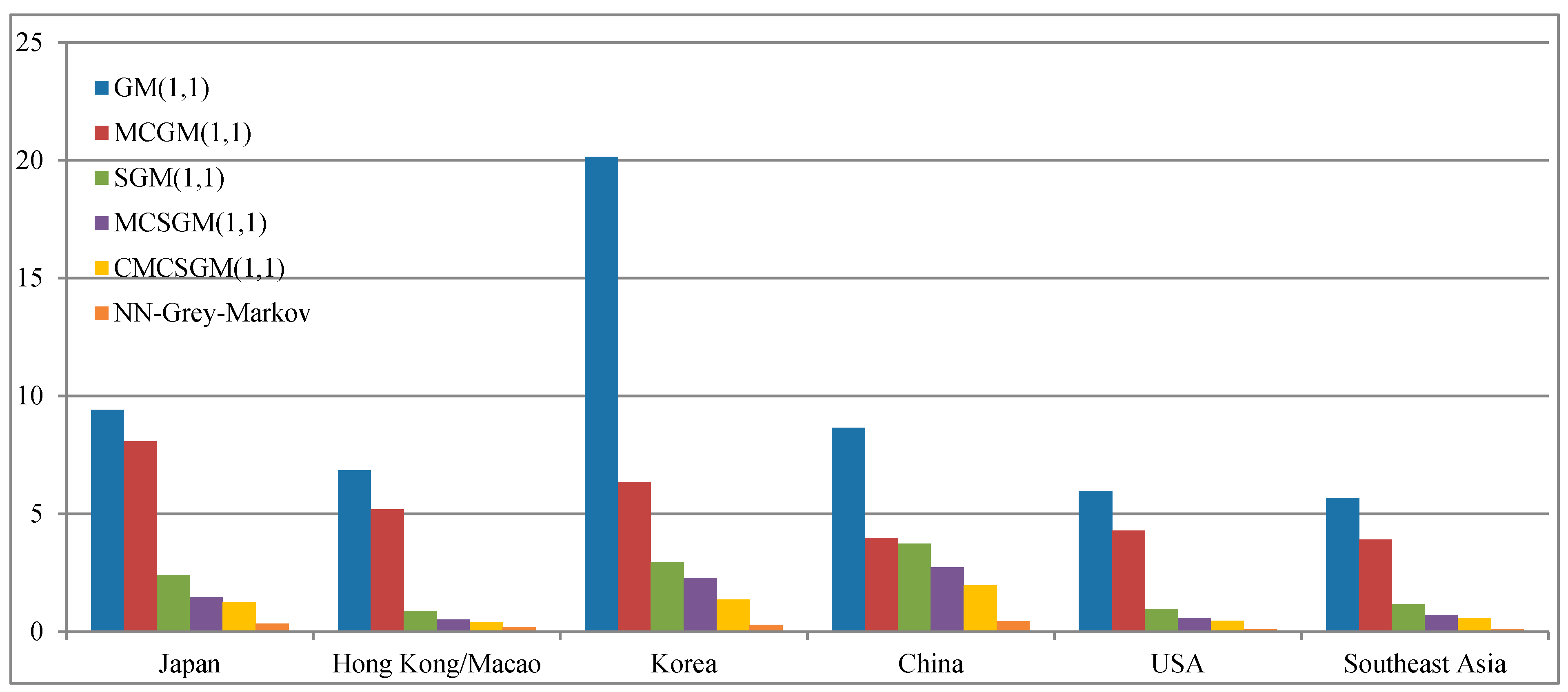
Figure 1. Model-fitting results for Case I.
Information 08 00126 g001
Figure 2. Testing results for Case I.
Information 08 00126 g002
Figure 3. Model-fitting results for Case II.
Information 08 00126 g003
Figure 4. Testing results for Case II.
Information 08 00126 g004
Table 1. Historical annual foreign tourists from six countries to Taiwan.
YearJapanHong Kong/MacaoKoreaChinaU.S.A.Southeast Asia
2001976,750435,16485,744 348,808488,968
2002998,497456,55483,624 377,470530,319
2003657,053323,17892,893 272,858457,103
2004887,311417,087148,095 382,822568,269
20051,124,334432,718182,517 390,929636,925
20061,161,489431,884196,260 394,802643,338
20071,166,380491,437225,814 397,965700,287
20081,086,691618,667252,266329,204387,197725,751
20091,000,661718,806167,641972,123369,258689,027
20101,080,153794,362216,9011,630,735395,729911,174
20111,294,758817,944242,9021,784,185412,6171,071,975
20121,432,3151,016,356259,0892,586,428411,4161,132,592
20131,421,5501,183,341351,3012,874,702414,0601,261,596
20141,634,7901,375,770527,6843,987,152458,6911,388,305
20151,627,2291,513,597658,7574,184,102479,4521,425,485
20161,895,7021,614,803884,3973,511,734523,8881,653,908