Article

Socioeconomic Covariate-Dependent Bayesian Nonparametric Mixture Model for Household Spending Patterns to Identify Multidimensional Vulnerability

1
Faculty of Information Science and Technology, Multimedia University, Jalan Ayer Keroh Lama, Melaka 75450, Malaysia
2
Centre for Advanced Analytics, COE for Artificial Intelligence, Multimedia University, Melaka 75450, Malaysia
3
Faculty of Management, Multimedia University, Jalan Multimedia, Cyberjaya 63100, Malaysia
4
Centre for Management and Marketing Innovation, COE for Business Innovation and Communication, Multimedia University, Cyberjaya 63100, Malaysia
*
Author to whom correspondence should be addressed.
Information 2026, 17(5), 459; https://doi.org/10.3390/info17050459
Submission received: 22 March 2026 / Revised: 26 April 2026 / Accepted: 5 May 2026 / Published: 9 May 2026
(This article belongs to the Special Issue Machine Learning and Data Analytics for Business Process Improvement)

Abstract

Household vulnerability assessment in Malaysia has traditionally relied on income-based indicators, which do not adequately capture multidimensional deprivation. To address this limitation, this study employs Random Tree–Dirichlet Process Mixture Model (RT-DPMM) to identify latent heterogeneity in spending patterns and their associated socioeconomic characteristics. Using microdata from Household Expenditure Survey (HES), this study performs clustering on 5130 stable household head samples with nine spending proportional features to model their joint distribution as mixtures of Dirichlet distributions, while five socioeconomic covariates inform cluster allocation through Random Tree embeddings. The proposed RT-DPMM identifies four distinct spending clusters: Balanced Budget Households (Cluster 1, N = 2883), Mobility and Home-Support Households (Cluster 2, N = 642), Basic Essentials-Focused Households (Cluster 3, N = 977), and Luxury Households (Cluster 4, N = 628). Cluster 1 and 3 are characterized as relatively vulnerable groups. These clusters have lower income levels and allocate a larger budget share in Food and Beverages, consistent with the Engel Law’s interpretation of higher food percentage in lower income households. Cluster 1 households primarily allocate their budget evenly across essential and non-essential spending. Cluster 3 are mostly elderly household heads with the highest budget shares in essential spending. In contrast, Cluster 2 and 4 appear relatively better off financially, given their higher income and larger spending share to non-essential categories. These findings suggest that social assistance policies should target expenditure patterns, rather than relying solely on income-based targeting.

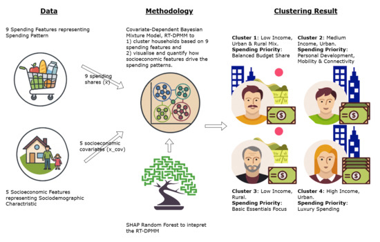
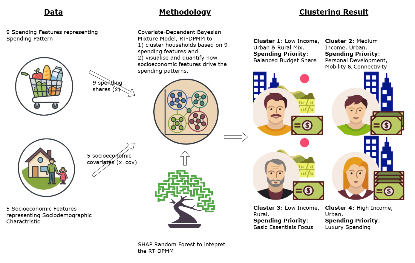
Graphical Abstract

1. Introduction

Poverty is increasingly recognized as a multidimensional phenomenon rather than a solely income-based measure. In Malaysia, the official Multidimensional Poverty Index (MPI) was introduced in 2015 as a complement to traditional income-based measures under the Eleventh Malaysia Plan (MP11) [1]. This framework covers three dimensions: education, health, and living-standard deprivations [2,3], emphasizing that poverty is far more complex than low income alone [4,5]. International studies have found that some individuals are multidimensionally deprived even when they are above the income poverty line [6], reflecting the importance of assessing vulnerability across multiple dimensions.
Economists have long argued that household consumption expenditure often provides a more accurate picture of household living standards than income. Firstly, households tend to smooth consumption using savings, whereas income may vary seasonally or be under-reported [7,8]. Several local studies have analyzed household poverty and inequality from a consumption expenditure perspective, but these are mainly conducted at an aggregate level [9,10]. For instance, Ref. [9] analyzed overall per-capita consumption expenditure inequality and its sociodemographic drivers, while [10] applied both linear and machine learning models to estimate overall consumption expenditure and its sociodemographic determinants, and found that variables such as age exhibit an inverted U-shaped nonlinear relationship with consumption expenditure.
A more informative analysis involves examining consumption expenditure at a disaggregated level to better understand household living standards. This represents a monetary view of living standards, where the analysis not only considers purchasing power but also evaluates whether households meet essential expenditure needs such as food and housing [11]. Aggregate consumption measures may conceal vulnerable households; for example, a household may be classified as non-poor overall but still be deprived in key areas if large share of its budget is absorbed by housing costs and constrain expenditure on food. In this study, we refer to this disaggregated composition of household consumption expenditure as the household spending patterns. In addition, multidimensional vulnerability refers to household deprivation assessed jointly across household spending pattern (monetary value) and socioeconomic characteristics (non-monetary value), aligning closely with the three core dimensions of the United Nation (UN)’s MPI (standard of living, health, and education). The former captures household expenditure allocations across essential and non-essential categories including health and education spending, while the latter incorporates income, education level, household size, age, and residential strata as proxies for the standard of living dimension.
Beyond the monetary perspective, recent studies have documented the use of sociodemographic variables as predictors in regression models to estimate their effects on consumption expenditure [12,13,14,15]. Nevertheless, a more holistic approach is to use these variables to explain the variations in spending behavior. Studies examining the relationship between socioeconomic drivers and spending patterns have gained increasing international attention in recent years [16,17], yet remain limited in the local literature. Existing Malaysian studies either treat overall consumption expenditure as a single dependent variable [9,10] or focus on a single Classification of Individual Consumption According to Purpose (COICOP) category at a time [13,14].
Generally, most of the local and international studies discussed above rely on regression techniques, treating income, consumption expenditure, or related poverty measures as dependent variables and household socioeconomic factors as determinants, with relatively little attention given to clustering approaches [18]. Clustering methods used predominantly rely on classical parametric techniques such as K-means or hierarchical clustering, which require pre-specifying the number of clusters or using heuristic methods such as the elbow criterion [18]. In contrast, Bayesian nonparametric approaches allow the data to determine the number of clusters. A common algorithm in this class is the Dirichlet Process Mixture Model (DPMM), implemented via a stick-breaking construction. Moreover, Bayesian methods provide probabilistic household-to-cluster assignments, capturing uncertainty that frequentist approaches typically overlook. In this context, a DPMM model can capture the joint distribution of households’ disaggregated consumption expenditures to cluster households with similar spending profiles together.
To incorporate socioeconomic variables, we adopt a covariate-dependent DPMM, specifically the single-atom-dependent formulation introduced by [19]. In this framework, all the clusters are defined as mixture components (atoms) shared across a common set of spending profiles, while household assignment probabilities vary with socioeconomic characteristics through a covariate-dependent weight function. In this context, socioeconomic variables are first mapped into a Random Tree embedding layer that captures nonlinear relationships and produces a high dimensional sparse matrix of the covariates. These matrix representations are then transformed into a dense vector and fed into a logistic stick-breaking that defines the covariate-dependent mixture weights within the DPMM. We refer to this specification as the Random Tree-dependent Dirichlet Process Mixture Model (RT-DPMM). This model enables the segmentation of households into latent spending clusters, addressing two key questions as follows:
  • What are the spending patterns of the latent clusters?
  • How do socioeconomic factors influence the probability of a household belonging to each spending-pattern cluster?
The proposed model demonstrates novelty in joining nonparametric clustering over disaggregated spending variables with the integration of socioeconomic covariates through an embedding layer within a coherent Bayesian framework. To the best of our knowledge, no prior Malaysian study has employed such an advanced mixture model to link household socioeconomic characteristics with spending patterns. Furthermore, the incorporation of forest-based machine learning models to create a nonlinear-based weight function within a unified Bayesian mixture modeling framework remains relatively unexplored in the context of household expenditure pattern analysis.
In summary, several gaps remain in the literature motivating this research. First, Malaysian poverty studies predominantly rely on aggregate income or consumption measures to assess household vulnerability. Although some studies conceptualize poverty as a multidimensional phenomenon, there is limited work examining disaggregated consumption expenditure to identify multidimensionally deprived households based on spending patterns. Second, Bayesian nonparametric clustering frameworks remain underutilized in this domain, despite their suitability for uncovering latent household groups that correspond to multidimensional vulnerability. This study aims to identify associations between household socioeconomic factors and spending patterns. By integrating disaggregated consumption expenditure features and modeling socioeconomic factors as covariates within the proposed RT-DPMM, this research seeks to fill these gaps and provide interpretable clustering results that can inform targeted policy interventions based on household spending behavior and socioeconomic characteristics.

2. Materials and Methods

2.1. Overview of Study

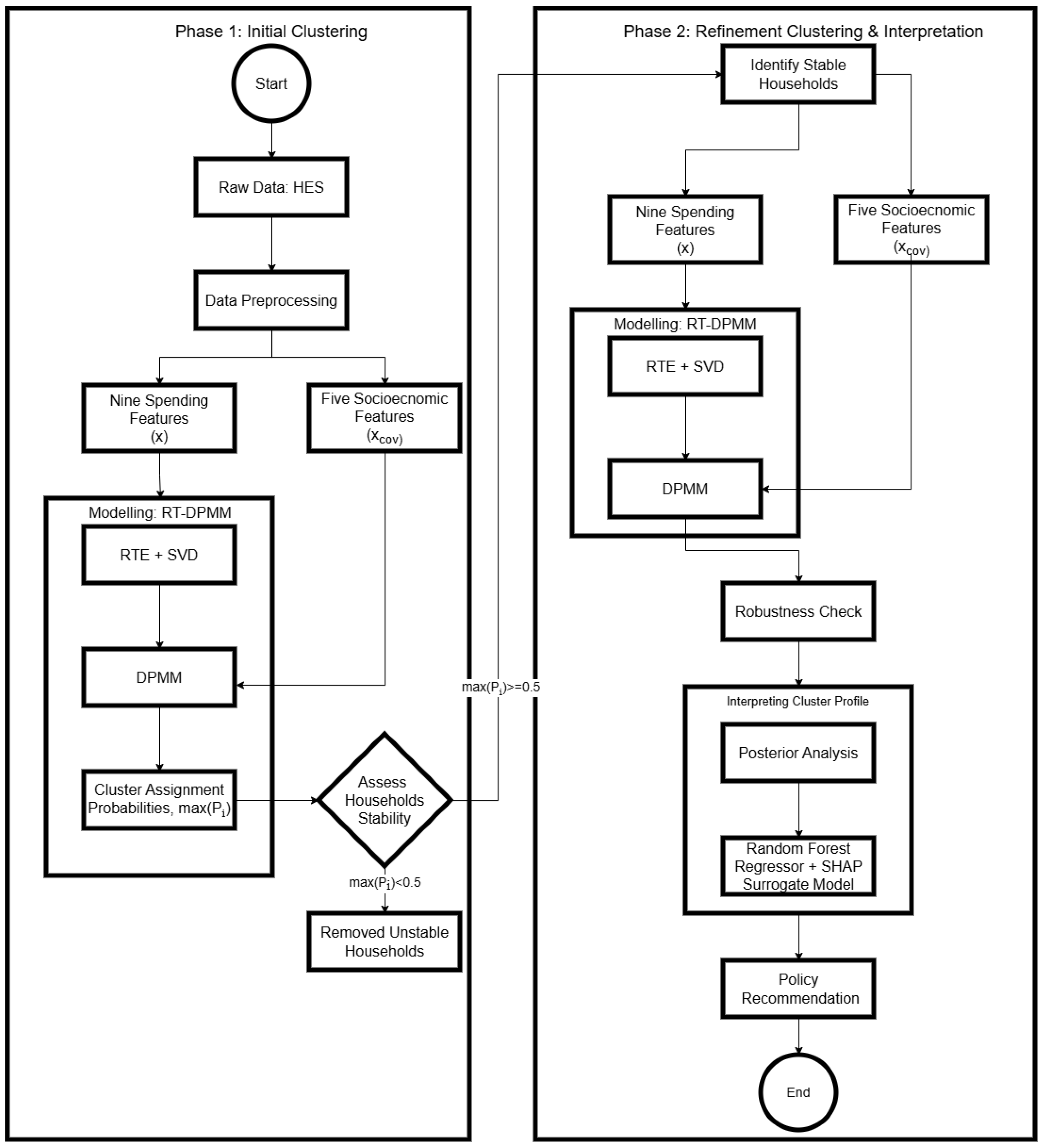
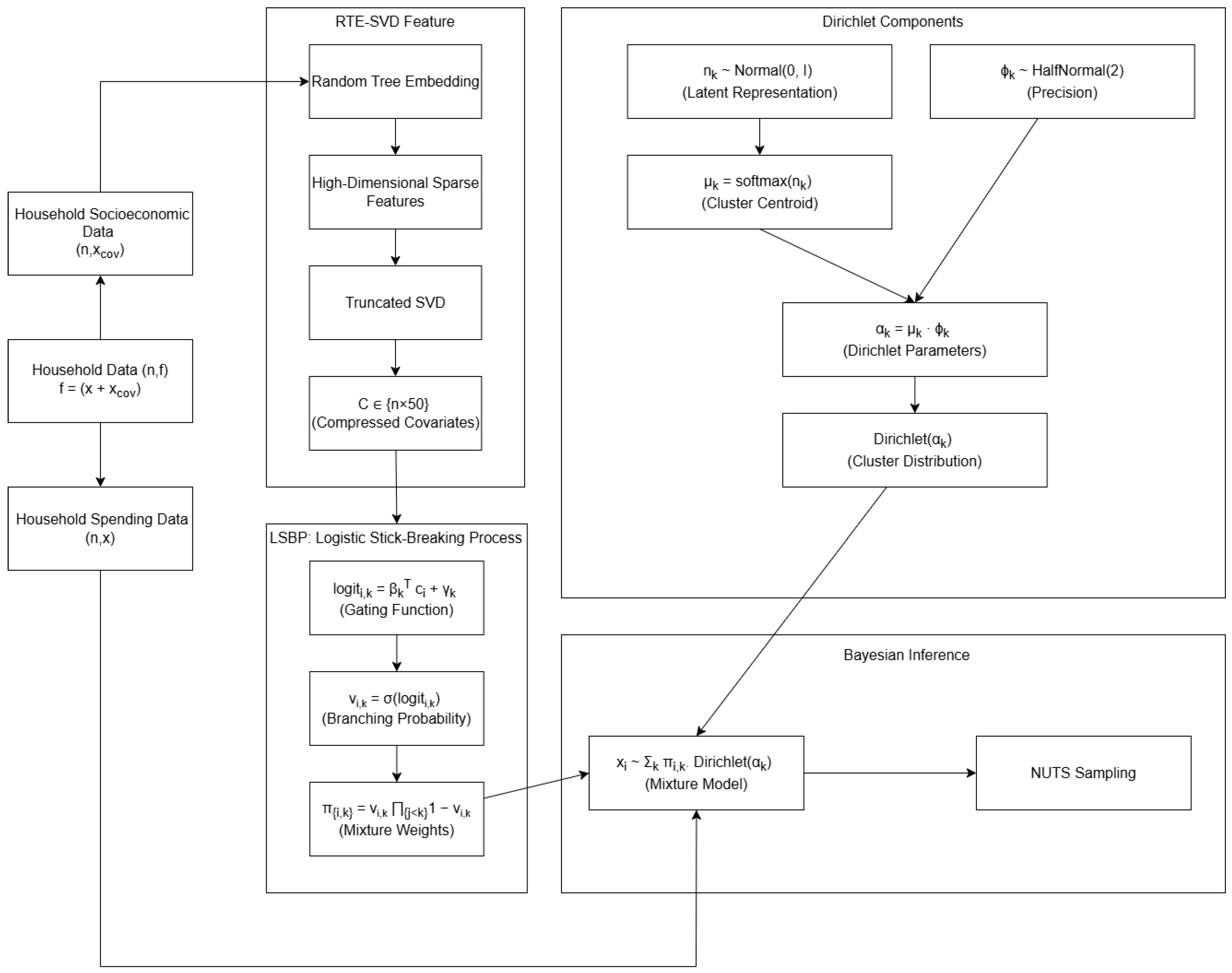
Figure 1 provides a flowchart illustrating how the experiment was conducted. The experiment adopts an iterative refinement strategy to identify and exclude unstable households in Phase 1, which may otherwise lead to convergence difficulties in estimating the model parameters. Algorithm 1 presents pseudocode and Figure 2 presents a schematic diagram for the RT-DPMM model specification applied in Phase 2 to stable households identified through the procedure as discussed in Figure 1.
In Phase 1, several preprocessing steps were applied to produce two feature sets for each household head: (i) nine spending proportion features (denoted by x), and (ii) five socioeconomic covariates (denoted by x cov ). Within the RT-DPMM framework, the socioeconomic covariates were transformed using Random Tree embedding (RTE) followed by Truncated Singular Value Decomposition (SVD) to form a dense continuous covariate vector consisting of 50 features. This transformed covariate vector, together with the nine spending features, was then used as input to the RT-DPMM, and posterior inference was performed to compute household-level cluster assignment probabilities. Households with a maximum posterior assignment probability P i < 0.5 are classified as unstable and filtered out because no single cluster received majority posterior support for that household [20].
In Phase 2, all the remaining households were refitted using the RT-DPMM, and the resulting posterior distributions were evaluated to ensure model robustness. Cluster spending patterns were interpreted based on posterior draws of the model parameters. To further interpret the effects of socioeconomic covariates on cluster assignment probabilities, a Random Forest regressor was trained as a surrogate model to directly map the original five socioeconomic covariates as independent variables to the mixture weights, used as dependent variables in a multi-output regression setting. Subsequently, SHAP (SHapley Additive exPlanations) was applied to the trained Random Forest surrogate model to interpret and explain how socioeconomic factors drive cluster assignment probabilities for the active clusters. Covariate contributions were visualized and quantified using feature importance bar plots and partial dependence plots (PDP).
Algorithm 1: RT-DPMM Specification presented in Pseudocode
  • Input:
  • X : n × 9 matrix of household spending proportions, where each row sums to 1.
  • C : n × 50 compressed socioeconomic profiles obtained from RTE-SVD.
  • K = 8 : maximum number of latent spending clusters (truncation level).
  • Output: Posterior distributions.
  • Part A: RT-DPMM Model Specification
  • Step 1 —Compute household-specific cluster weights via LSBP. For each household i and cluster k, a branching probability v i , k ( 0 , 1 ) is derived from socioeconomic profile c i , then converted to mixture weights π i , k via stick-breaking such that k π i , k = 1 .
  • for each cluster k = 1 , , K 1 do
    |       logit i , k = β k c i + γ k       v i , k = σ logit i , k ( 0 , 1 )
    end
                π i , k = v i , k · j < k 1 v i , j , such that k = 1 K π i , k = 1
                β k j N ( 0 , 0.5 ) , γ k N ( 0 , 1 )
  • Step 2—Define the spending profile of each cluster under mean–precision parameterization. Centroid μ k represents the average spending allocation of cluster k, while precision ϕ k controls how tightly households concentrate around it.
  • for each cluster k = 1 , , K do
    |       n k N ( 0 , I d )       μ k = Softmax ( n k )       ϕ k HalfNormal ( σ = 2 )       α k = μ k · ϕ k
    end
  • Step 3—Specify the observed spending likelihood as a weighted mixture of cluster-specific Dirichlet distributions with household-specific weights from Step 1.
                x i k = 1 K π i , k · Dirichlet ( α k )
  • Step 4—Perform Bayesian inference via NUTS sampler (2 chains, 2000 warm-up + 4000 draws; convergence criterion.

2.2. Data Preprocessing

This study utilized micro-level household data from the Household Expenditure Survey (HES) 2022 administrated by Department of Statistics Malaysia (DOSM). There are 13 household consumption expenditure features that capture how a household spends on different goods and services monthly. This disaggregated level of 13 consumption expenditure features is known as Malaysian Classification of Individual Consumption According to Purpose (M-COICOP) which follows the United Nations COICOP [21]. Additionally, HES also captures several household socioeconomic features. All the 13 M-COICOP features and five socioeconomic factors were selected in this study. The five socioeconomic factors selected and their ranges are as follows:
  • Income: RM320.06–RM38,344.08.
  • Age of Household Head: 15–98.
  • Household Size: 1–21.
  • Education Level of Household Head: 1–7 (The higher the number, the higher the education level).
  • Strata (Urban Ref.): 0–1 (A value of 1 denotes household living in urban).
Based on evidence from recent local studies of household socioeconomic determinants of overall consumption expenditure using HES data from different years, these studies strongly support these five socioeconomic factors as significant determinants of household spending power [9,10]. In a later modeling phase, these socioeconomic variables will be transformed into a high-dimensional and sparse matrix vectors; thus, selecting five socioeconomic variables is a safe choice to prevent computational complexity and adding more insignificant socioeconomic variables may not increase the explanatory power.
HES data comprises both household-level and individual-level records. As the 13 M-COICOP features are recorded as household-level, this study selected only household heads as the representatives for each household in order to ease the subsequent interpretation to the reference individual across households of different sizes. Given this, the actual spending by a household head must be calculated after considering the household size. Simply dividing the income and 13 M-COICOP features by number of individuals living in a household (divisor) is not ideal as household head (adult) tends to be allocated more resources. For this purpose, this study computed the divisor using the Oxford Equivalence Scale [22] as shown in Equation (1):
S i = 1.0 + 0.7 ( N adults 1 ) + 0.5 ( N children )
where N adults is the number of adults (age 18 ) including the household head and N children is the number of children (age < 18 ) in a household. The first adult was weighed at 1.0, subsequent adults was weighed at 0.7, and children at 0.5. The 13 M-COICOP and income features were then transformed into per-capita scale using this adjusted-divisor. Households with total consumption expenditure (calculated as total of 13 M-COICOP features) higher than 95th percentiles were considered as outliers and discarded in this study. In this stage, 14,268 households observation were selected, and Table 1 shows the descriptive statistics of the 13 M-COICOP and five socioeconomic features. In the rest of this paper, references to ’household’ should be read as referring to the household head that represents a particular household.
As presented in Table 1, most of the M-COICOP features have zero values, but cannot simply be dropped. This prevalence of zero values will distort the probabilistic model built in the later analysis. To mitigate this, selected pair of M-COICOP features were merged to reduce the sparsity caused by excessive zero values, and thus ensure the pairings are conceptually meaningful based on their similar roles in household budgeting:
  • Discretionary Spending: Alcoholic Beverages and Tobacco + Restaurant and Accommodation Services to capture discretionary spending.
  • Household Operation: Furnishing, Household Equipment, Routine Household Maintenance + Personal Care, Social Protection and Miscellaneous Goods and Services to capture personal, shelter and maintenance costs.
  • Personal Development: Recreation, Sport and Culture + Education to capture human capital and leisure investment.
  • Mobility and Connectivity: Transport + Information and Communication to capture social interaction.
This aggregation reduced the 13 M-COICOP to nine spending features. This significantly reduces the amount of zero values. To further ensure no zero values lie in any nine spending features, households with any zero value under these nine features were excluded. In this stage, the household head samples left were 11,374 (retaining 79.7% of the original 14,269).
The nine expenditure features were transformed into a proportion scale. This was done by dividing the absolute spending value of each spending feature by total expenditure (sum of nine spending features) to obtain proportions ranging from 0 to 1. The continuous socioeconomic features (Per Capita Income, Education Level, Household Size, Age) were standardized, while the binary variable ‘Strata’ remained untouched. Table 2 shows again the descriptive statistics of the retained 11,374 household heads that were used in the modeling part with no zero values left in the nine spending and five socioeconomic features. We refer to x as the nine spending features and x cov as five socioeconomic features.

2.3. Transforming Socioecnomic Features

Worldwide studies have well documented the nonlinear relationships between socioeconomic factors and consumption expenditure [23,24], and this is further supported by a local study using the same HES 2022 dataset [10]. This study employed Random Tree embedding (RTE), an unsupervised case of Random Tree [25] to capture the complex and nonlinear relationships between these x cov , and transform the socioeconomic covariates into a high-dimensional sparse binary representation, where the dimensionality is equal to the total number of leaves of all the trees. One can view this representation as households (rows) assigned to different leaves (columns), so household with similar socioeconomic profiles should have assigned to similar leaves.
The raw sparse representation of x cov is computationally expensive to use directly as an input in the Bayesian model. To handle this sparse x cov , Truncated SVD is applied to transform it into a lower-dimensional dense x cov . This effectively preserves the main structural information of the socioeconomic profiles while reducing the input dimensions to a tractable level, thereby improving the computational efficiency and enhancing the convergence stability of the MCMC sampler.

2.4. Random Tree-Dependent Dirichlet Process Mixture Model (RT-DPMM)

This study develops a novel hybrid Bayesian model that integrate the Random Tree embedding with covariate-dependent DPMM model (RT-DPMM) to cluster household based on their spending patterns. The proposed RT-DPMM model is capable of addressing the problem domain of this study through three mechanisms. First, the model leverages the dense x cov within the stick-breaking process. As explained earlier, the dense representation of x cov captures the interactions within socioeconomic features interactions, allowing the model to reflect the nonlinear relationships between socioeconomic covariates, x cov and latent spending clusters instead of directly model x cov within stick-breaking process which treat them linearly. Second, we utilized the Dirichlet distribution for the mixture component since the x is in a proportion scale. Dirichlet distribution is a perfect candidate as it aligns with our study design where each household head’s spending features sum up to exactly 1. Finally, we implemented a covariate-dependent Logit Stick-Breaking Process (LSBP) as the proposed model’s stick-breaking process. This algorithm offers two key advantages: First, it allows the number of spending clusters to grow infinitely (theoretically) without bound, instead of imposing predetermined a fixed number of cluster. Second, it ensures that the probability of cluster assignment is conditioned on x cov . The details of proposed RT-DPMM are described in the following section.

2.4.1. Mixture Likelihood (Check Mixture Weight or Cluster Assignment Probs)

Since each row in spending features x is compositional (sum to 1), likelihood is modeled as Dirichlet mixtures. The mean–precision parameterization is utilized for interpretability of latent spending clusters. For a specific cluster k, it has a Dirichlet distribution as its component with a centroid parameter μ k and a precision parameter ϕ k .
Suppose that each household is i; we can denote its spending features as x i , and corresponding socioeconomic features dense x cov covariates as c i . Therefore, the likelihood for x i is given by Equations (2) and (3) below:
x i k = 1 K π k ( c i ) Dirichlet ( α k ) ,
α k = μ k · ϕ k ,
where π k ( c i ) is covariate-dependent mixture weight representing the probability that household i is generated from cluster k given its socioeconomic covariates c i , unlike standard DPMM model which assumes global mixture weights shared across for all the households. Furthermore, α k is decomposed into two interpretable components where μ k represents the component centroid of cluster k which is expected value of the x i for any household assigned to cluster k, and ϕ k controls the compactness of the cluster. The component centroid μ k directly inform the average spending pattern of household assigned to cluster k. A higher ϕ k indicates that households in the cluster k are tightly concentrated around the centroid μ k .

2.4.2. LSBP—A Covariate-Dependent Stick-Breaking Process

The construction of LSBP is originally proposed by [26] that extend the constructive definition of the Dirichlet Process [27] by replacing the beta-distributed breaking variables with logistic regression functions so the mixture weight π k vary with covariates c i . Specifically, this is the single-atom DDP application of LSBP [19,28]. In single-atom DDP, the cluster components Dirichlet ( α k ) are shared globally but the mixture weight π k ( c i ) are dependents on socioeconomic covariates c i . The novelty of our RT-DPMM is the usage of the nonlinear RTE as the input covariates for the LSBP. This hybrid combination of nonlinear machine learning embedding and Bayesian model (RT-DPMM) ensure household-specific mixture weights π k ( c i ) are determined based on the nonlinear interactions of socioeconomic factors, overcoming the linearity constraints of the standard logistic regression used in the stick-breaking process.
For each cluster k (with a truncation level of K), we defined a conditional branching probability. This represents the prior probability of household i being generated from cluster k in the stick-breaking sequence, given it was not allocated to any earlier cluster j < k . Equation (4) show how the branching probability is computed using a logistic regression as defined by [26]
v i , k = σ ( β k c i + γ k ) ,
where σ ( · ) is the sigmoid function, β k is the vector of regression coefficients linking the socioeconomic covariate c i to cluster k, and γ k is the cluster-specific intercept.
The mixture weight π k ( c i ) is defined as Equation (5) below:
π k ( c i ) = v i , k j = 1 k 1 ( 1 v i , j ) ,
where the j = 1 k 1 ( 1 v i , j ) represents the remaining probability mass available after accounting for Cluster 1 through k 1 . This formulation ensures that the sum π k ( c i ) is 1 for every household, and the most crucial property is the probability that a household belonging to a specific latent spending cluster is now explicitly driven by their unique socioeconomic covariates c i .

2.4.3. Hyperparameter Prior Specification and Inference Settings

We assigned weakly informative priors to the hyperparameters of the proposed RT-DPMM. The prior distributions used in this study are as follows:
Component Centroid ( μ k ): We model the unconstrained cluster n k using a weakly informative Normal prior of μ = 0 and σ = 1 , which is then transformed to component centroid μ k using the SoftMax function. Equation (6) shows the idea:
n k Normal ( μ = 0 , σ = 1 ) and μ k = Softmax ( n k ) ,
Component Precision ( ϕ k ): The Half-Normal prior constrains precision to be positive. A scale of σ = 2 is a suitable weakly informative Half-Normal prior where the sampler can explore the cluster variance freely. Equation (7) shows the idea:
ϕ k HalfNormal ( σ = 2 ) ,
Beta Coefficients ( β k j ): We apply a regularizing prior with σ = 0.5 to the regression weight. Since the socioeconomic covariates c i remains a high-dimensional embedding (50 features), and this prior specification prevents the model from assigning extreme odds ratios to features. Equation (8) shows the idea:
β k j Normal ( μ = 0 , σ = 0.5 ) ,
Intercepts ( γ k ): A weakly informative Normal prior of μ = 0 and σ = 1 is used for the intercepts. Equation (9) shows the idea:
γ k Normal ( μ = 0 , σ = 1 ) ,
We tested the truncation level of cluster K = [ 8 , 10 , 12 , 15 , 20 ] , which is computationally efficient and sufficient for this domain. The posterior distributions were estimated using No-U-Turn Sampler (NUTS) implemented in PyMC library with a Blackjax backend, running 2 chains of 2000 tunes + 4000 draws to ensure convergence.

2.5. Hungarian Algorithm to Detect Label Switching

A fundamental challenge in Bayesian mixture modeling is the label switching problem [29]. This happens when the MCMC sampler explores symmetric modes of the posterior distribution invariant to the permutation of cluster indices, causing the cluster labels to swap randomly across chains. To resolve this, a post-processing re-labeling strategy is employed based on the Hungarian Algorithm [30] to align all the clusters in chain 1 using chain 0 as reference.
We defined a reference configuration based on the first chain. As there are 2 chains, we computed the optimal permutation σ * that minimizes the Squared Euclidean distance between chain 1’s cluster centroids μ k and the reference centroids of chain 0. The cost minimization is solved via the linear assignment problem as shown in Equation (10) below:
σ * = arg min σ S K j = 1 K μ j ref μ σ ( j ) chain ,
where S K denotes the set of all the possible permutations of the indices { 1 , , K } . The term μ j ref μ σ ( j ) chain represents the Euclidean distance between the centroid of cluster j in the reference chain (Chain 0) and the centroid of the cluster assigned to index j by permutation σ in the target chain. The optimization finds the specific mapping σ * that minimizes the total aggregate distance between the two sets of cluster centroids.
Once the optimal permutation σ * is identified, this mapping is applied globally to all the posterior samples within chain 1. After this relabeling, the labels of all the latent clusters are consistent across two chains and safe to proceed to the posterior analysis.

2.6. Interpreting Socioeconomic Covariates Effect via Explainable Random Forest Regressor

Apart from interpreting the cluster spending patterns via component centroid μ k , we also aimed to quantify and visualize the relationships between household socioeconomic factors c i and the mixture weight π k ( c i ) as estimated by the RT-DPMM. One of the easiest ways is to simply summarize the descriptive statistics across household assigned to active clusters but this approach will limit the analysis of relationships and determination of the exact magnitude of how covariates drive the mixture weight. Although the LSBP in Equation (4) is structurally interpretable (one can simply read the β k to understand the magnitude and direction of covariates’ effects). In this implementation, the covariates c i is an RTE–SVD embedding rather than by the original human-readable variables. Therefore, reporting the numerical values of β k does not directly translate into policy-relevant insights such as how the income of a household head affects its probability of being assigned to active clusters.
For this reason, we further developed a surrogate model (Random Forest regressor + SHAP) to map the original five socioeconomic covariates x cov to the sticks v i , k which are then used to compute mixture weight π k ( c i ) outcome using Equation (5). Random Forest was selected to capture nonlinearities and higher-order interactions without explicit feature engineering and handle outliers. Another important reason for selecting Random Forest is that both RTE and Random Forest are tree-based ensemble methods that partition the covariate space via decision trees. RTE is an unsupervised method to produces leaf nodes, while Random Forest is a supervised method that maps socioeconomic covariates to mixture weight. Using similar method to reconstruct the relationships can best recover the information represented in RTE–SVD embedding. Since the predictive outcome v i , k is continuous, thus a Random Forest Regressor is built. This model also supports the fitting of multiple continuous targets simultaneously, so it can directly fit v i , k as the target variables.
After fitting the Random Forest, we used SHAP (SHapley Additive exPlanations) values to decompose the covariates’ contribution over the predictions [31]. SHAP determines global feature importance by calculating the mean absolute SHAP value across all the observations, thereby quantifying the average marginal contribution of each covariate to the prediction. To interpret the result, feature importance bar plot was used to evaluate the importance of five socioeconomic covariates for each active cluster and the partial dependence plot to visualize the relationship between socioeconomic covariates and cluster memberships.

2.7. Robustness Check

To ensure the reliability of the discovered consumption patterns, we conducted a rigorous two-step validation process focusing on MCMC convergence and the decisiveness of household-to-cluster assignments.

2.7.1. MCMC Convergence Diagnostics

The most important evaluation is the convergence status of the posterior distribution across chains. The R-hat statistic is used to assess whether the independent MCMC chains meet convergence. A R-hat value of 1.0 indicates perfect convergence, while R-hat < 1.05 are generally acceptable [32,33]. We also reported the Effective Sample Size (ESS) in two forms: ESS (bulk), which measures sampling efficiency across the bulk of the posterior distribution, and ESS (tail), which assesses the reliability of tail quantile estimates. Both values required values of at least 100, with higher values indicating more reliable posterior summaries [33].

2.7.2. Assessing Model Fit Through Posterior Prediction

To assess the model’s goodness-of-fit, we performed Posterior Predictive Checks [32]. This process involves generating synthetic datasets x rep from the posterior predictive distribution, which marginalizes over the uncertainty in the model parameters θ . Equation (11) shows the idea:
p ( x rep x ) = p ( x rep θ ) p ( θ x ) d θ ,
where p ( x rep θ ) is the likelihood of the replicated dataset, given model θ and p ( θ x ) is the posterior distribution of parameters given the observed data x. The marginal density of the observed spending pattern against posterior predictive draws is plotted. This visual check assesses the robustness of RT-DPMM in reproducing the key features of the observed spending pattern x and thus the model can be generalized for predicting new households.

2.7.3. Unstable Assignment and Iterative Refinement

Apart from statistical convergence of parameters, we also evaluated the uncertainty of the cluster assignments for each household. Since the proposed RT-DPMM is a soft clustering method, it is possible for a household to have ambiguous cluster membership. For example, with a truncation level of K = 8 , a household might be assigned to Cluster 1 with a probability of 0.4 while simultaneously holding a probability of 0.35 for Cluster 2. In such cases, while the household is technically “assigned” to Cluster 1, it is weak and statistically unstable. We referred to such households as unstable.
To identify unstable households, we computed Max Posterior Probability ( P i ) of a household i, defined as the maximum expected assignment probability across all the clusters. Equation (12) below presents the idea:
P i = max π ¯ i , k ,
where π ¯ i , k is the posterior mean probability of all the MCMC samples of household i belonging to cluster k and P i is simply the largest π ¯ i , k value among the K clusters. Based on this metric, we applied an iterative refinement strategy as described in Section 2.1. Households with P i < 0.50 were classified as unstable and removed. The RT-DPMM was then re-fit using only stable households.

3. Results

3.1. Construction of Latent Socioeconomic Features via RTE-SVD

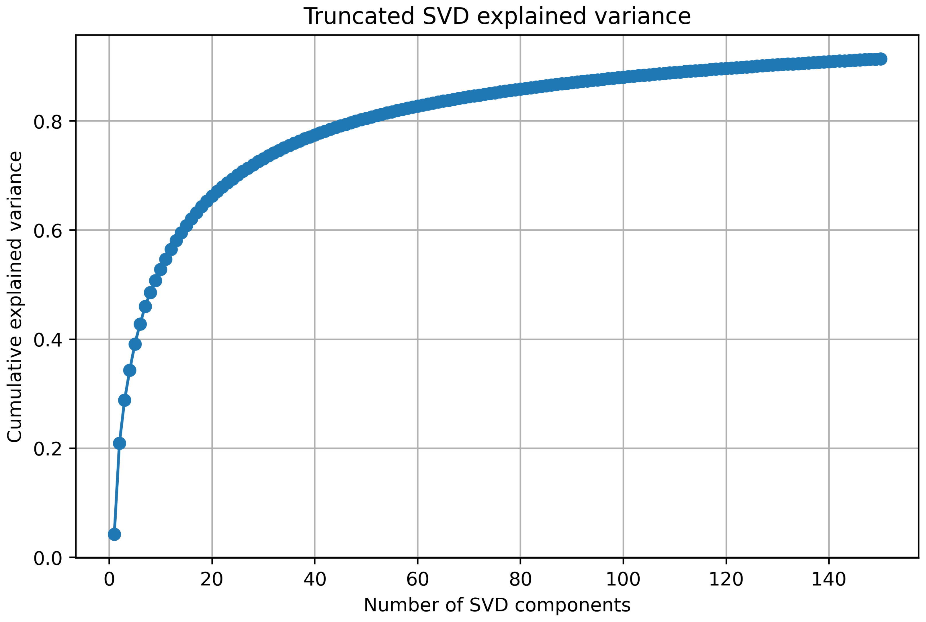
Table 3 presents the parameter settings and number of features used in our RTE and SVD. We specified 200 trees and a maximum of 32 leaf nodes per tree to produce a sufficiently high-dimensional sparse representation with 5356 features. This feature repsentation captures nonlinear interactions among the five socioeconomic covariates while ensuring embedding stability given the low input dimensionality of x cov . The sparse x cov (5356 features) produced by RTE is transformed into a continuous dense x cov using truncated SVD. Figure 3 presents the cumulative explained variance of the components using truncated SVD. As illustrated in Figure 3, 50 components capture about ∼80% of the total variance in the sparse x cov . This is an optimal trade-off between variance explained and computational cost to reduce original 5356 sparse features into only 50 features while effectively eliminating noise. The marginal gain in explained variance diminishes significantly after 50 so we ended up with selecting 50 components. The resulting dense representation x cov is then served as the input to the RT-DPMM in the subsequent stage.

3.2. Model Diagnostics and Validation

Before analyzing the posterior distribution to understand cluster spending pattern, we evaluated the statistical reliability of the RT-DPMM using the convergence and goodness-of-fit metrics.

3.2.1. Comparison with the Baseline DPMM

Prior to presenting the RT-DPMM results, we first fitted a standard Dirichlet Process Mixture Model (DPMM) as a benchmark to compare its empirical performance with the proposed RT-DPMM. Following [34], the infinite mixture was operationalized via a finite truncated stick-breaking approximation, where the K-th breaking variable was deterministically set to v K = 1 . The concentration parameter was specified as α Gamma ( 1 , 1 ) .
This baseline DPMM shares the same Dirichlet mixture likelihood, mean–precision parameterization of the component centroids μ k , truncation level K = 8 , and nine spending features as the proposed RT-DPMM.
The principal distinction between the two models lies in the construction of the mixture weights. In the baseline specification, the stick-breaking process generates a single global weight vector that is shared identically across all the household observations n. The formulation is given by
v k Beta ( 1 , α ) , π k = v k j = 1 k 1 ( 1 v j ) ,
where π k denotes the global weight for cluster k, without an observation-specific index i (in contrast to Equations (4) and (5) in the RT-DPMM). Under this construction, the cluster assignment probability for cluster k is identical for every household, irrespective of socioeconomic characteristics.
Empirically, the baseline DPMM did not perform satisfactorily in our study for two principal reasons. First, the Markov Chain Monte Carlo (MCMC) chains exhibited convergence issues. The global weight parameters π = ( π 1 , , π K ) —derived from the stick-breaking draws v k —and the component centroid parameters μ k both recorded R-ha statistics exceeding the acceptable threshold of 1.05. This indicates that the two MCMC chains converged to qualitatively different posterior solutions, characterized by differing numbers of active clusters and distinct global weight configurations.
This lack of convergence suggests that meaningful clusters are not identifiable when relying solely on a single global stick-breaking weight construction. In contrast, the proposed RT-DPMM, which incorporates both spending and socioeconomic covariates in the mixture weight construction, achieved stable convergence and well-defined clusters.
This empirical failure is theoretically coherent and consistent with the prior literature [35,36]. Through simulation experiments, the study found that when informative covariates are omitted from the mixture weight specification, inferential performance may deteriorate substantially [36]. They further show that covariate-dependent mixture models can produce improved clustering performance when relevant covariates influence the latent allocation mechanism. In particular, the LSBP is identified as a flexible and high-performing implementation of covariate-dependent weight construction. Hence, the empirical instability of the baseline DPMM and the supporting theoretical evidence motivate the adoption of the covariate-dependent RT-DPMM in this study. By incorporating socioeconomic characteristics into the mixture weight structure, the RT-DPMM provides a more coherent and robust framework for modeling the complex heterogeneity in Malaysian household spending patterns.

3.2.2. Filtering Unstable Households

Following the iterative refinement strategy, we first filtered out all those unstable households mentioned in Section 2.7.3. About ∼55% of the households were classified as unstable ( P i < 0.5 ) and filtered out. After filtering these observations, we refitted the RT-DPMM using only stable households (5,132 samples). Using iterative refinement strategy, most of the model parameters met convergence, and most important components’ centroid parameter μ k met perfect convergence.

3.2.3. Sensitivity to Truncation Level

To assess the robustness of the proposed RT-DPMM to the choice of truncation level, we also fitted the model under five truncated K = [ 8 , 10 , 12 , 15 , 20 ] . The purpose is to examine whether the latent clusters structure are stable across different levels of truncation in terms of the number of active clusters, the estimated cluster centroids, and the associated socioeconomic covariates.
Empirically, the model produced highly consistent results across four truncation levels K = [ 8 , 10 , 12 , 15 ] . In all four cases, the posterior distribution converged to the same substantive solution, with four active clusters, similar component centroids μ k values, similar socioeconomic characteristic. We further observed that the convergence behavior of the component-centroid parameters was most favorable at K = 8 , where all the R-hat values for μ k attained the perfect convergence value of R-hat = 1.00. As the truncation level increased, the convergence diagnostics gradually became less stable, and ultimately failed to converge at K = 20 . This suggests that excessively large truncation levels will only introduce unnecessary posterior complexity and incorrect clustering solution.
Overall, these results indicate that the RT-DPMM is robust over a reasonable range of truncation values. Since the clustering structure, component centroids, and socioeconomic profiles remained consistent for K = 8 , 10 , 12 , and 15. Given this result, the remaining paper focuses on discussing the clustering outcomes under K = 8 . The detailed comparison of four active spending clusters across all four truncation settings is discussed in Appendix A.1 (Table A1, Table A2, Table A3, Table A4, Table A5).

3.2.4. Identification of Active Clusters and MCMC Convergence

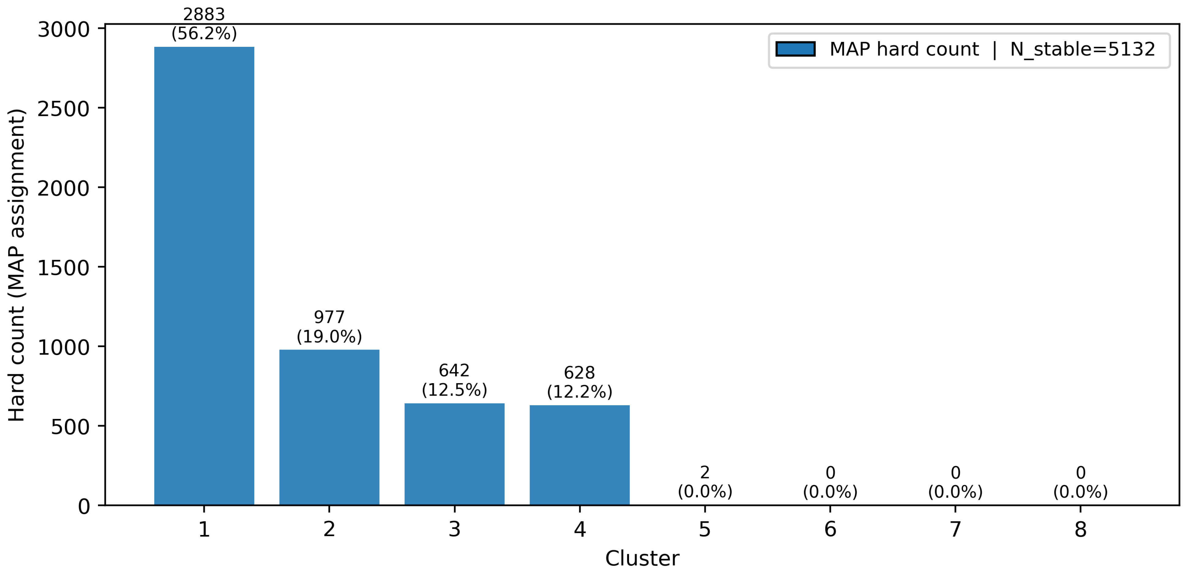
A key advantage of the Dirichlet Process is its ability to determine the number of clusters nonparametrically. Using a truncation level of K = 8 , the RT-DPMM yielded four active clusters, with posterior expected counts concentrated in Clusters 1–4. Figure 4 presents the posterior expected number of households for each cluster. As illustrated in Figure 4, household heads assigned concentrated heavily on first four clusters. Cluster 1 is the dominant cluster with 2883 household heads. Cluster 2, 3 and 4 records substantially fewer households. Cluster 5 is almost inactive with only two household heads assigned, and is therefore not considered further in the analysis. The remaining three clusters have zero household heads. Given this result, the remainder of this paper focuses on the four active clusters (Cluster 1, 2, 3, and 4), which contain a total of 5130 stable households.
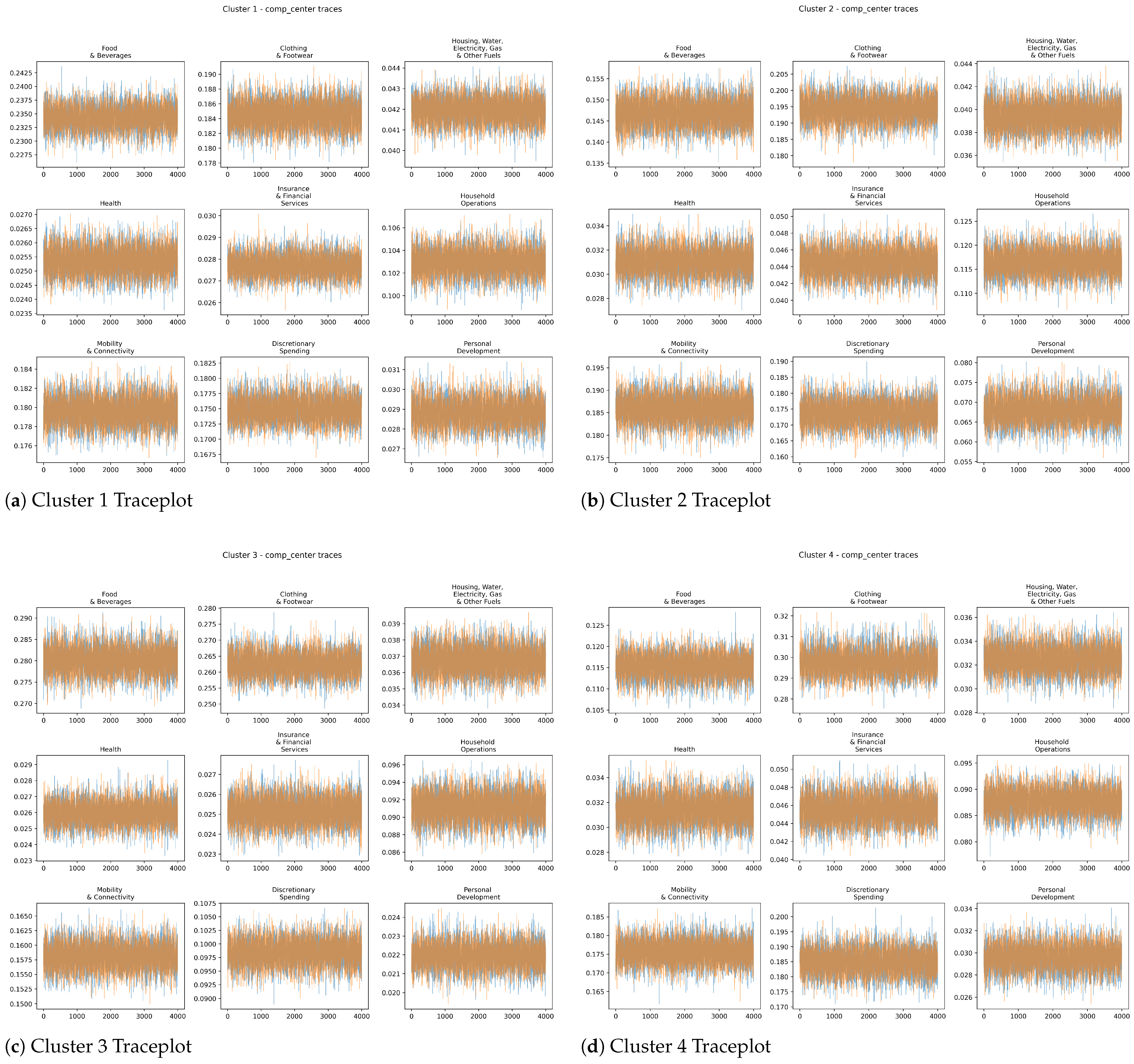
The convergence of the model parameters was assessed using the R-hat diagnostic. Despite the truncation level being set to K = 8 , the model converged to a parsimonious solution with only four active clusters (Cluster 1, 2, 3, and 4) capturing the household population. As summarized in Table 4, the centroid parameters μ k for these four active clusters demonstrated robust stability, with all of them having R-hat values of ≤1.00 and both ESS (bulk) and ESS (tail) record very high values, satisfying standard convergence criteria [32,33]. The traceplots for component centroid ( μ k ) parameters can be found in the Appendix A.2 (Figure A1).

3.2.5. Posterior Predictive Checks

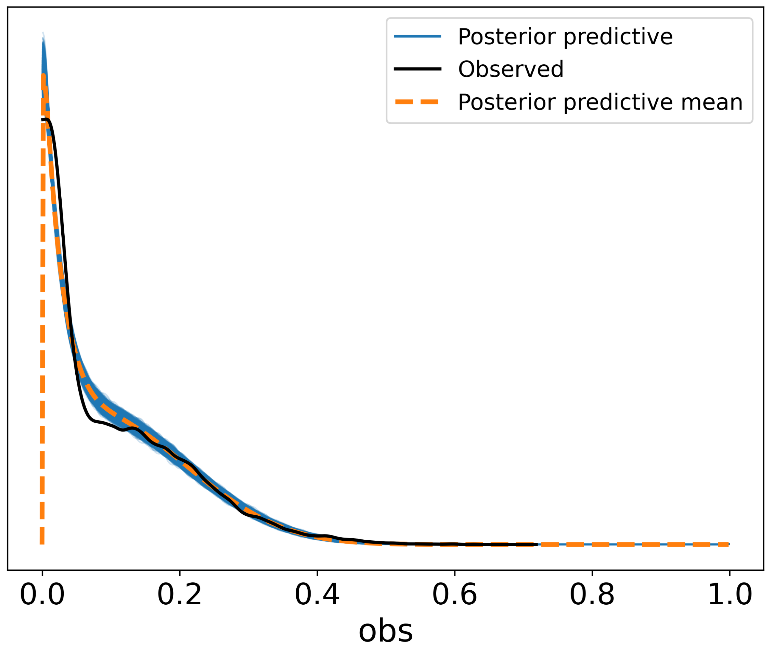
Figure 5 presents the global goodness-of-fit of the RT-DPMM. The black line denotes the observed empirical marginal density, the blue line denotes the posterior predictive distribution based on the draws from the model, while the orange line represents the posterior predictive distribution mean. As illustrated in Figure 5, the proposed model successfully reproduces the observed distribution of expenditure shares. The close alignment between observed values (black line) and the posterior predictive distribution (orange and blue lines) shows that RT-DPMM adequately models heterogeneity in household spending patterns across the household head observations.

3.3. Cluster Spending Pattern

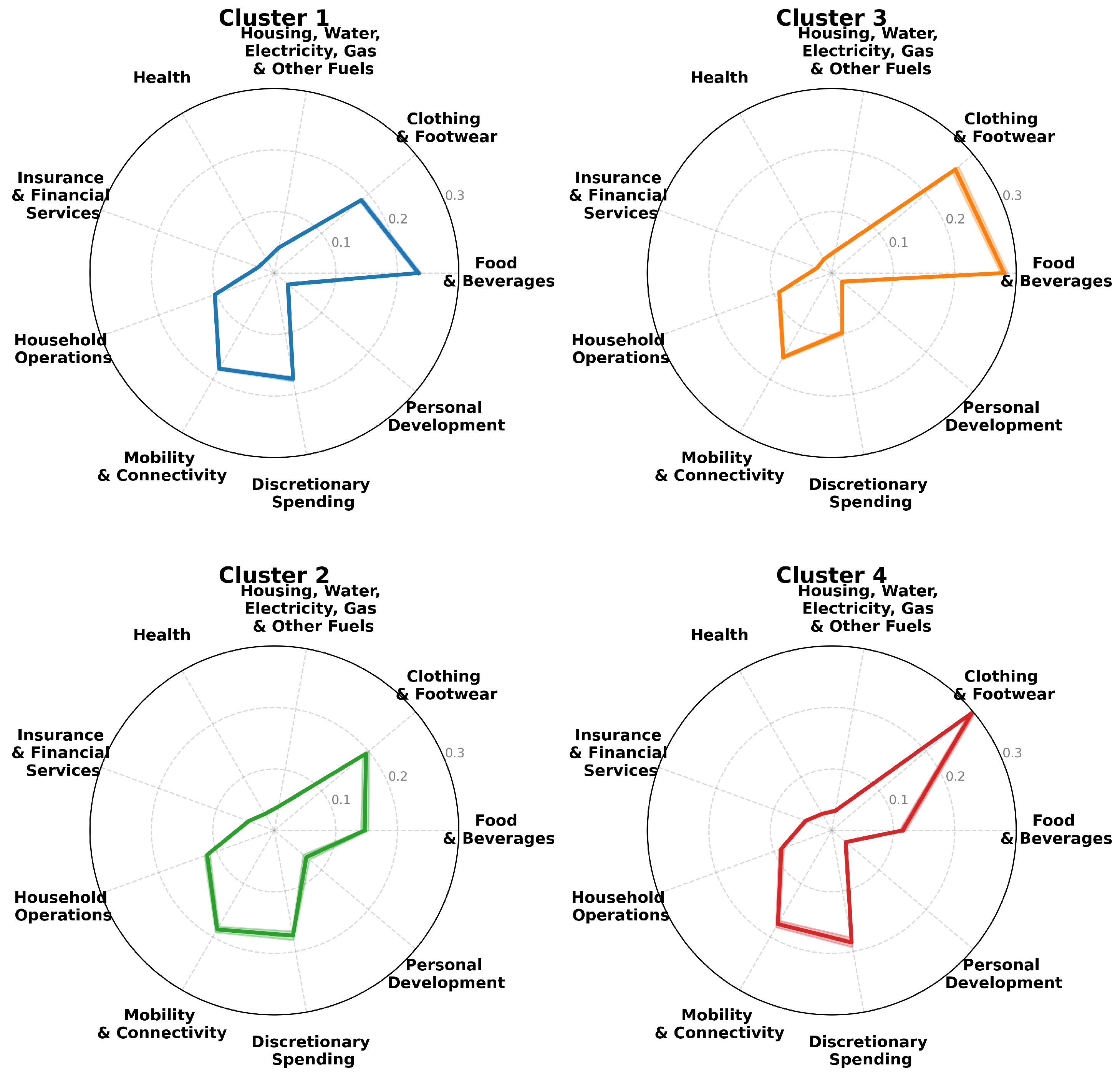
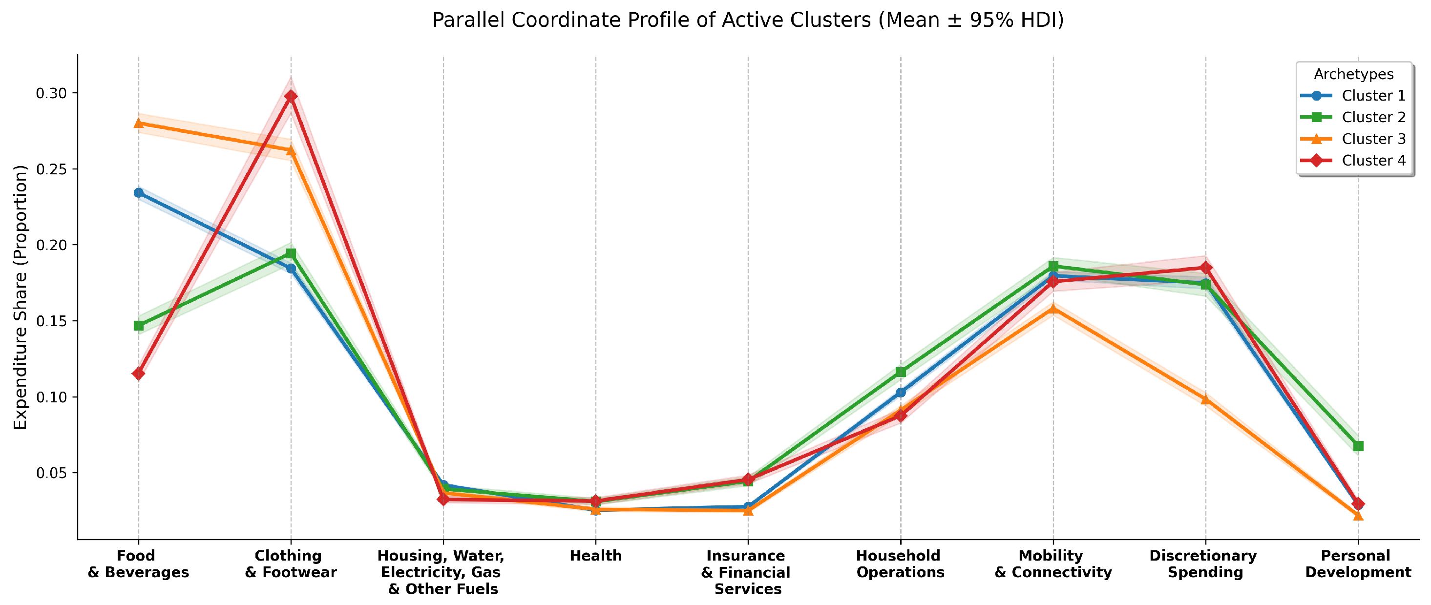
The proposed RT-DPMM effectively segmented the Malaysian household records into four distinct clusters. We characterized these profiles by examining their centroid parameters’ component centroids, μ k , by reporting their mean and 95% HDI bound. To visualize the multidimensional differences, Figure 6 presents radar plots of the spending pattern for the four active clusters. We utilized this visualization because the distinct geometric shapes generated by the radar plots allow for an immediate, intuitive comparison of the structural differences in budgeting priorities across groups, highlighting trade-offs that might be obscured in standard bar charts. On the other hand, Figure 7 presents a parallel coordinate plot that presents the cluster profiles side-by-side, to highlight the difference across spending features. Complementing these visual plots, Table 4 also provides detailed numerical summary of the component centroids, μ k . As shown in Table 4, the model demonstrates high precision in estimating these profiles, with narrow HDI bounds indicating that the spending behaviors of each cluster are well-defined and statistically distinct.
Overall, the four clusters show distinct priorities in household budgets. Each cluster was assigned a title and interpreted based on their spending priorities:
  • Balanced Budget Households (Cluster 1): Households living in this cluster spend mostly on Food and Beverages (0.234), while notable shares go towards Mobility and Connectivity, Clothing and Footwear, Discretionary Spending and relatively small shares towards other spendings. In short: this cluster is characterized by balanced budget share with a slightly strong emphasis on Food and Beverages and moderate share on other non-essential spendings.
  • Mobility and Home-Support Households (Cluster 2): Households living in this cluster show a relatively balanced profile with elevated spending on Mobility and Connectivity (0.186), Clothing and Footwear (0.194) and Discretionary Spending (0.174). The budget allocated to Food and Beverages is low (0.147). Notably, the spending on Personal Development is the highest (0.068) among the four clusters.
  • Basic Essentials-Focused Households (Cluster 3): Households living in this cluster spend mostly on essential categories: the largest shares on Food and Beverages (0.280) and Clothing and Footwear (0.262). Spending on Mobility and Connectivity and Household Operations are moderate. Other categories record a smaller share.
  • Luxury Households (Cluster 4): Households in this cluster spend mostly on Clothing and Footwear (0.297) and show highest Discretionary Spending share among the four clusters (0.185), with substantial allocations also to Mobility and Connectivity (0.176) and Household Operations (0.088). Spending on Food and Beverages (0.115) is the lowest among four clusters.

3.4. Interpreting Covariates’ Effect—A Descriptive Approach

Table 5 presents descriptive statistics of the original scale of five socioeconomic factors across four representative clusters (Clusters 1, 2, 3 and 4). Household observations (N), median, mean, and standard deviation (std) are reported in each cluster.
Cluster 1 is characterized by low per-capita income (mean of RM1721.09), larger household size (mean of ∼5) and lower education level (mean of ∼3). Cluster 3 exhibits a similar profile to Cluster 1 but has slightly lower per-capita income (mean of RM1529.11), smaller household size (mean of ∼4) and a similar education level (mean of ∼3). Both clusters have nearly identical number of household heads from both urban and rural areas (given that the mean of 0.50 from Cluster 1 and 0.39 from Cluster 3). Household heads from Cluster 2 appear to have a higher standard of living with per-capita income (with mean of RM3973.26) and higher education level (mean ∼4), which is substantially higher compared to those observed in Clusters 1 and 3. Household heads in Cluster 2 tend to be larger with mean household size of approximately five members (mean ∼5). Household heads in the last cluster, Cluster 4, are characterized by the highest per-capita income (mean of RM6255.19), smallest household size (mean of ∼2) and highest education level (mean of 4.76). Generally, household heads assigned to Cluster 2 and 4 are also urban residents (mean of 0.92 from Cluster 2 and mean of 0.98 from Cluster 4). Regarding the age of household heads, Cluster 4 records the lowest value (mean of ∼41), followed by Cluster 2 and 1 (mean of ∼45 and ∼47 respectively). Cluster 3 records at highest age with approximately 51 years (mean of ∼51).
After interpreting their socioeconomic features, we could then link the cluster spending pattern identified (see Section 3.3) with their respective socioeconomic characteristics. For instance, the Balanced Budget Households cluster (Cluster 1) is associated with low per-capita income and education level, while the Luxury Households cluster (Cluster 4) is associated with high per-capita income and education level. Note that this interpretation only provides descriptive statistical way of interpreting such associations between spending pattern of socioeconomic characteristics. For a deeper understanding of these associations, further analysis to examine how socioeconomic characteristics of household heads influence cluster assignment probabilities by quantifying their effects using feature importance bar plots and partial dependence plots will be provided in next section.

3.5. Interpreting Covariates’ Effect via Explainable Random Forest Regressor

We used the Random Forest + SHAP surrogate model described in Section 2.6 to investigate the five socioeconomic covariates’ effect on mixture weight. As the Random Forest is independently trained using original scale of five socioeconomic features x cov and logit sticks v ( i , k ) , which are later computed to get mixture weights π k ( c i ) , the goodness-of-fit must also be evaluated before moving on to interpret the model.
Table 6 shows the R-squared and Root Mean Squared Error (RMSE) using five-fold cross validation, in which the R-squared between the actual and predicted logit sticks across four active clusters are very similar (R-squared of 1 indicate perfect match between observed and predicted values) and low RMSE means that the model’s predictions are, on average, close to the actual observed values.
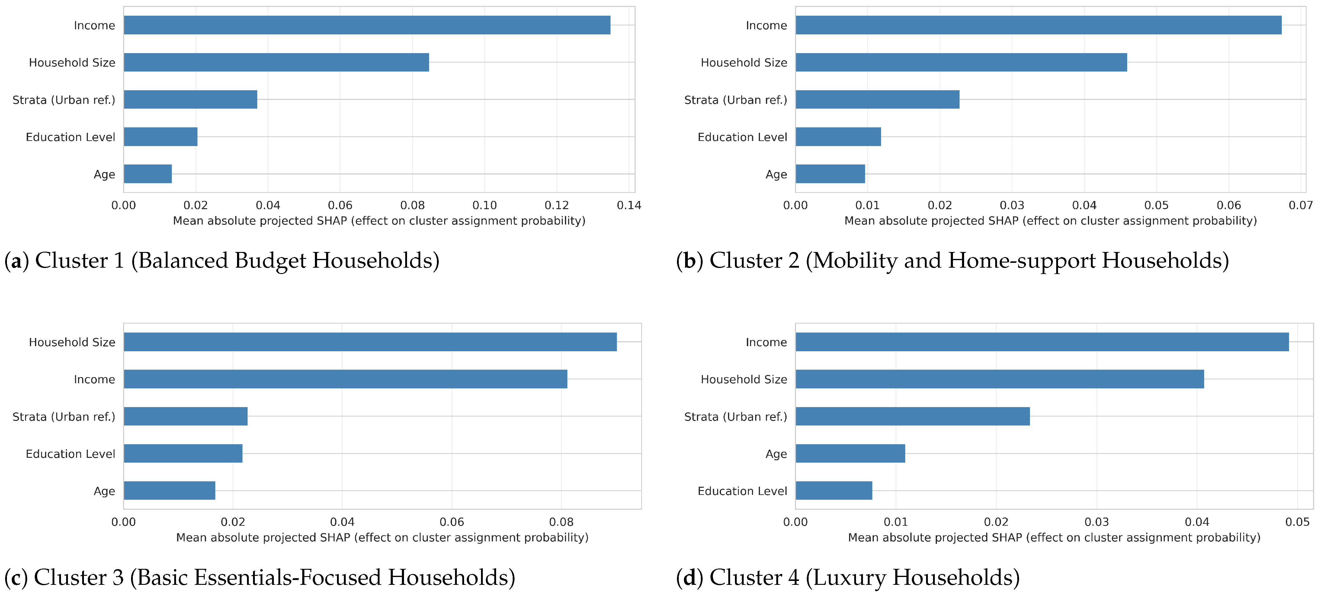
Figure 8 shows four feature importance bar plots for four active clusters. These bar plots rank the feature importance of five socioeconomic covariates across clusters from top (highest mean absolute SHAP value) to bottom (lowest mean absolute SHAP value). The higher the mean absolute SHAP value (x-axis), the stronger the socioeconomic feature. Overall, the five socioeconomic covariates do not contribute equally toward clusters as the ranking and mean absolute SHAP value vary across clusters, but income consistently ranks as the most-important feature and household size as the second-most-important feature. Strata (Urban ref.), education level and age have relatively less contribution. A summary of how socioeconomic factors affect household head assignment probabilities toward each cluster is given below:
  • Figure 8a Cluster 1 (Balanced Budget Households): Per-capita income is the most-important predictor to determine the probability of household heads falling into this cluster (mean absolute SHAP value of ∼0.14). Household size contributes moderately (∼0.08). The rest of the socioeconomic factors are less important.
  • Figure 8b Cluster 2 (Mobility and Home-support Households): Per-capita income ranked as the first-most-important feature and household size as second-most-important features but with mean absolute SHAP value of ∼0.07 and ∼0.05 respectively, compared to a big gap of per capita income (∼0.14) and household size (∼0.08) as observed in Cluster 1.
  • Figure 8c Cluster 3 (Basic Essentials-Focused Households): The mean absolute SHAP values among per capita income and household size are minimal (both are close to ∼0.08). This means household size share similar importance with per capita income in determining a household head’s probability to be assigned to this cluster.
  • Figure 8d Cluster 4 (Luxury Households): The overall bar plot pattern is similar to Cluster 2, but the mean absolute SHAP value across the socioeconomic factors are different.
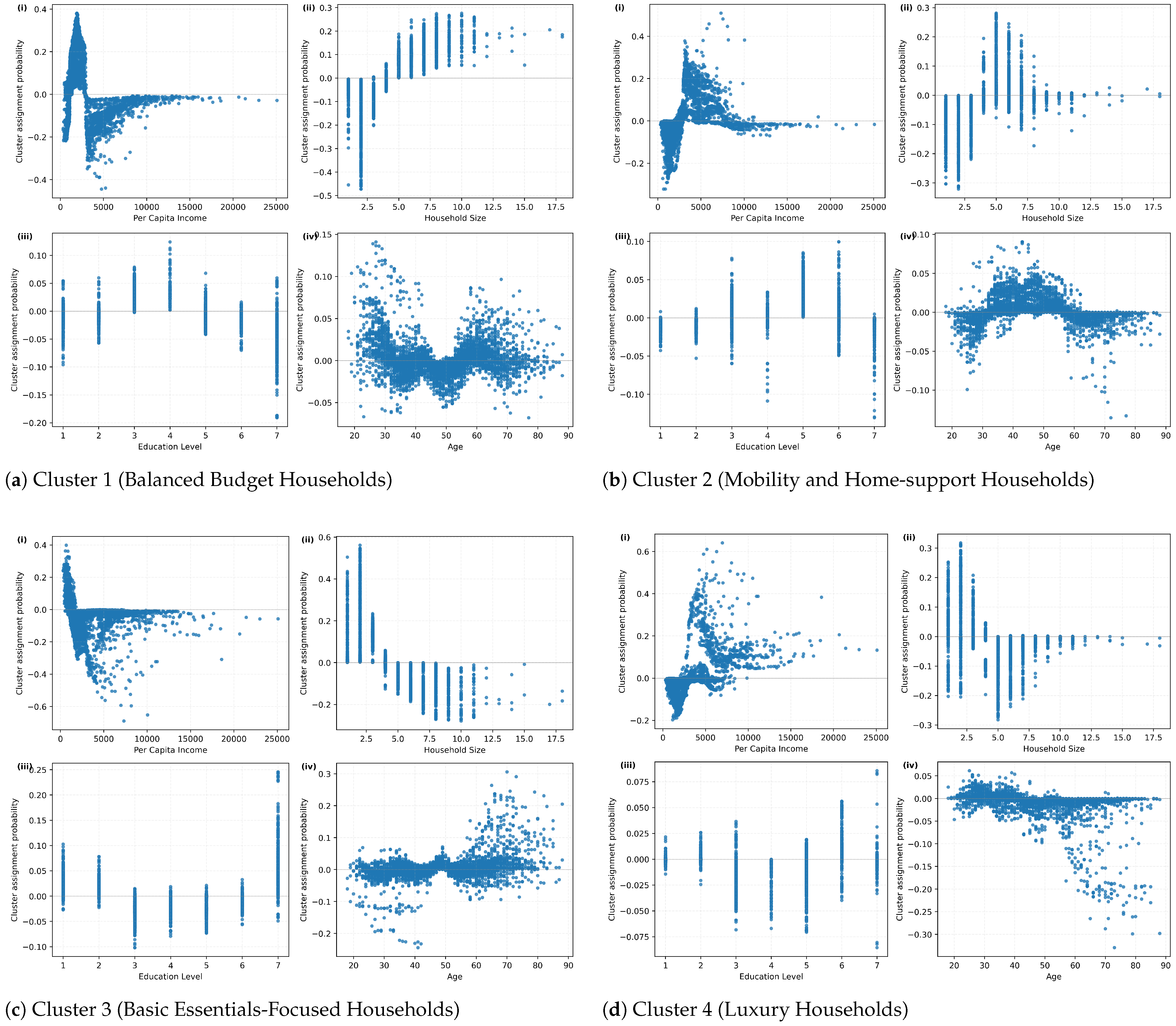
Figure 9 shows four SHAP partial dependence plots (PDPs) for each cluster, in a total of 16 PDP across four socioeconomic covariates. PDP is an important visualization method used in our study as the socioeconomic factors may have nonlinear effect over cluster assignment probabilities. Section 4.2 will explain the findings by comparing how and why these socioeconomic covariates’ effects vary across the clusters.

4. Discussion

4.1. Understanding Cluster Spending Patterns

The proposed RT-DPMM segmented 5130 stable households into four clusters with distinct spending patterns and different socioeconomic profiles. The four representative clusters reveal substantial heterogeneity in how Malaysian households allocate their budgets across essential and discretionary spending categories. Cluster 1 (Balanced Budget Households, N = 2883) is the major cluster where households are characterized by high Food and Beverages shares (23.4%) and moderate allocations to Clothing and Footwear, Mobility and Connectivity, and Discretionary Spending. Analysing from socioeconomic profile, this cluster predominantly comprises low-income households (mean per-capita income of RM1721.09) with larger household sizes (mean of 5.28 members) and lower education levels (mean of 3.27). Cluster 3 (Basic Essentials-Focused Households, N = 977) exhibits similar economic profiles (mean per-capita income of RM1529.11) but different spending patterns. Households in this cluster are characterized by the highest shares allocated to Food and Beverages (28.0%) and Clothing and Footwear (26.2%) but the lowest share in Discretionary Spending (9.8%). This cluster’s households socioeconomic profile records a lower household size (mean of 4.01 members) and older household heads (mean age of ∼51 years). Combining the spending pattern and socioeconomic profile observed in Cluster 3, households living in this cluster can be regarded as focusing their spending on basic necessities (Food and Beverages + Clothing and Footwear). In contrast, Cluster 2 (Mobility and Home-Support Households, N = 642) and Cluster 4 (Luxury Households, N = 628) represent households with higher standard of living where they are characterized by higher per-capita incomes (RM39,732.26 and RM6255.19 respectively) and elevated education levels. These clusters typically allocate larger budget shares to some non-essentials categories such as Discretionary Spending, Mobility and Connectivity, and Personal Development and smaller budget shares on Food and Beverages, aligning with Engel’s law, which states that the proportion of income spent on food decreases as income rises [37].
Generally, both Cluster 4 (Luxury Households) and 3 (Basic Essential Focus households) record large Clothing and Footwear shares (29.7% and 26.2% respectively). This observation aligns with classical Engel-curve theory which also points out that spending share on Clothing and Footwear can vary across life cycle (age) and total resources (e.g, income) [38,39]. In addition, lower share of Food and Beverages are observed in Cluster 2 (14.7%) and Cluster 4 (11.5%), suggesting that these clusters are relatively financially-better-off clusters. In contrast, the higher food shares in Cluster 1 (23.4%) and Cluster 3 (28.0%) indicates these clusters are more budget-constrained and vulnerable.

4.2. Understanding How the Socioeconomic Characteristics Drive the Spending Patterns

4.2.1. Vulnerable Clusters: Cluster 1 and Cluster 3

The proposed RT-DPMM suggests that households with similar income levels may demonstrate varying spending patterns. For instance, per capita income of household heads in Cluster 1 and 3 with nearly identical mean incomes of RM1721.09 and RM1529.11 respectively, exhibits different spending behaviors and priorities. Cluster 1 allocates substantial shares to the Mobility and Connectivity and Discretionary Spending categories (18.0% and 17.5%) while Cluster 3 concentrates almost exclusively on Food and Beverages (28.0%) and Clothing and Footwear (26.2%) but not Discretionary Spending (9.8%). This is in contrast to traditional income classification systems, which provide an incomplete assessment of household vulnerability by failing to account for multidimensional spending behavior. Furthermore, Cluster 1 is categorized as larger household sizes, while Cluster 3 consists of smaller household sizes led by older household heads. In this context, unidimensional-based income classification would simply classify these households as within the same income group without further investigation of their current spending priorities. By contrast, the refined clusters proposed in this paper provide a more holistic understanding of household variability.
The SHAP PDP plot in Figure 9a (Cluster 1) and Figure 9c (Cluster 3), further reveal that households assignment probabilities to these clusters are driven by fundamentally different socioeconomic mechanisms despite both clusters being classified as vulnerable clusters with low incomes. Figure 9a(i) shows an inverted U-shaped relationship in Cluster 1, where assignment probability peaks at low-to-middle income and declines at both extremes, while Figure 9c(i) shows a near-linear negative relationship in Cluster 3, where the lowest-income households carry the highest assignment probability. This indicates that Cluster 1 predominantly captures middle-low income compared to very low income households in Cluster 3. From a spending pattern perspective, households in Cluster 3 with low income level spend almost exclusively on Food and Beverages and Clothing and Footwear, leaving minimal budget share for other non-essential spending categories. On the other hand, households in Cluster 1, with slightly higher income levels, are able to distribute their budget across both essential and non-essential categories.
Figure 9a(ii) shows that the cluster assignment probability are initially negative for small household sizes (sizes 2–4, SHAP values ranging from −0.5 to −0.2), and turn strongly positive for household size onward. This pattern suggests that Balanced-Budget Households are likely to belong to medium and large families and show their challenge of feeding multiple dependents with diverse spending priorities. Conversely, Figure 9c(ii) shows that Cluster 3 captures a close to linear negative relationship, which is also the steepest among all four clusters. Very small households (size 1 and 2) have high positive SHAP values (∼0.5), and as household size becomes larger, it eventually becomes negative (∼−0.2). This indicates that Basic Essentials-Focused Households typically belong to small household sizes, consistent with the interpretation that this cluster captures households comprising of the elderly (explained in next paragraph).
Figure 9a(iii) shows that the effect of education level on cluster assignment probability remains unclear at first (SHAP values range from ∼0.05 to ∼-0.05), and then eventually become positive and peak education level of 3 and 4 and decline in education level onward. On the other hand, Figure 9c(iii) presents a U-shaped trend where the cluster assignment probability initially captures a positive value (education level of 1), and then decreases to negative value but suddenly increases back to positive value at the highest education level. If we ignore the strange effects observed at the education level of 1 in both clusters, we may posit that lower education level tends to shape the households to spend evenly across essential and non-essential spending, while higher education level tends to shape spending pattern towards being focused on essentials. Such strange effects may be because education level here captures only household head but not the other family members.
Figure 9a(iv) shows that age has an unclear effect toward cluster assignment probability, with SHAP values oscillating around zero to slightly positive across as age increases. This unclear effect may suggest that Balanced Budget Households are driven primarily by other socioeconomic factors. Conversely, as shown in Figure 9c(iv), Cluster 3 demonstrates a clear positive relationship. The cluster assignment probability is initially negative (around −0.1 for ages 20–40), and then eventually increases to strongly positive values (∼0.3) for older ages (60+). Given this phenomenon, it can be concluded that households with Basic Essentials-Focused spending patterns are tightly linked to aging and retirement.

4.2.2. Financially Better-Off Clusters: Cluster 2 and Cluster 4

Cluster 2 and 4 represent households with higher standard of living, characterized by substantially higher mean per-capita incomes (RM3973.26 and RM6255.19 respectively) and lower Food and Beverages expenditure shares (14.7% and 11.5%), consistent with Engel’s law. Despite this shared economic advantage, households living in these two clusters exhibit distinct spending priorities too. Cluster 2 shows a relatively balanced profile with elevated spending on Mobility and Connectivity (18.6%), Clothing and Footwear (19.4%) and Discretionary Spending (17.4%), with notably the highest Personal Development share (6.8%) among all four clusters. Cluster 4, labeled as “Luxury Households,” allocates the largest shares to Clothing and Footwear (29.7%) and Discretionary Spending (18.5%) among all the clusters while maintaining the lowest Food and Beverages share (11.5%). This is opposed to Clusters 1 and 3, which concentrate heavily only on Food and Beverages, reflecting households living in this Cluster 4 have greater financial flexibility in adjusting and allocating their budget toward non-essential categories.
Further interpreting the SHAP PDP in Figure 9b (Cluster 2) and Figure 9d (Cluster 4), households assignment probabilities to Cluster 2 and 4 are also driven by different socioeconomic mechanisms despite both classified as higher-income clusters. Figure 9b(i) demonstrates a positive relationship where the cluster assignment probability increases as the income increase. The SHAP values are initially negative for low income and gradually increase as the income increases and peak at an income level near to RM3000, before falling rapidly later. This indicates that middle-income households are more likely to belong to Mobility and Home-Support Households. Figure 9d(i) demonstrates similar positive relationship, in the exception that households with income level of ∼RM3000 onwards show high positive SHAP values (peaking at ∼0.6) plus low negative SHAP values (∼0.2). This unclear relationship suggests that perhaps income is not the only key socioeconomic factor to determine whether households will be assigned to this Luxury cluster.
Figure 9b(ii) shows that in Cluster 2, the relationship between household size and cluster assignment probability appears to be negative, where small households (sizes 2–4) show negative SHAP values (∼−0.3), eventually increase to positive values (peaking at ∼0.3) for moderate household sizes (5–7), and then become negligible for households beyond that size. This pattern suggests that Mobility and Home-Support Households belong to medium-sized families. Conversely, Figure 9d(ii) exhibits a positive relationship. Small households (sizes 2–3) contribute to unclear (∼−0.2 to ∼0.3) but generally positive SHAP values, and then become negligible for household size onward. This indicates that small household sizes are strongly associated with luxury spending pattern.
Figure 9b(iii) shows that education level has a nonlinear effect on cluster assignment probability. The SHAP values initially remain near zero for lower education levels (1–2), and then increases and peak at ∼0.10 at moderate education levels (4–5) and finally decline at the highest education level (7). This link back to the highest spending observed in Personal Development among the four clusters, where highly educated households tend to favor investing in personal development while maintaining a moderate spending on essential and non-essential spending. On the other hand, Figure 9d(iii) reveals that education level has a confusing effect over cluster assignment probability, given that the SHAP values oscillate around zero. This suggests that education level is not a significant socioeconomic factor in explaining households’ spending behavior in terms luxury spending, as shown by the extreme values captured in Clothing and Footwear and Discretionary Spending. The weak and unclear education effects observed in both financially better clusters contrast sharply with the effect observed in vulnerable clusters, suggesting that the Luxury and Mobility and Home-Support clusters are primarily driven other socioeconomic factors.
Figure 9b(iv) shows that age has a relatively clear pattern in explaining the cluster assignment probability. Positive SHAP values are observed among middle ages (40–60), and negative values are found at the young (∼20–∼40) and elderly (∼60+). The pattern suggests middle-aged households are likely to be clustered as Mobility and Home-Support Households, potentially reflecting peak earning years and established mobility needs for commuting and family support activities. Similarly, Figure 9d(iv) shows a negative relationship where the SHAP values is initially positive for young households (∼20–∼35) with positive SHAP values (∼0.05), and then declines to negative values at ages onward. This suggest that young households in Cluster 4 are more likely to prioritize their spending on non-essential items such as Discretionary Spending and Clothing and Footwear.
Our disaggregated consumption approach addresses a critical gap identified in prior Malaysian studies. Existing research predominantly analyzes overall consumption expenditure as a single dependent variable [9,10] or examines individual M-COICOP division in isolation [13,14]. While nonlinear relationship is found between age and overall per capita consumption expenditure [10], this study reveals that the relationships between distinct spending patterns and socioeconomic features are even more complex. For instance, this study found that elderly households with lower per capita incomes are more likely to allocate their budget on essential spending while younger households tend to focus on non-essential spendings.

4.3. Policy Recommendations

This section discusses the results of four representative household clusters with heterogeneous spending patterns and socioeconomic profiles in terms of providing actionable insights for policies on cost-of-living and the well-being of Malaysians. Before discussing it, it is worth for us to revisit the social assistance programs in Malaysia such as financial aids that can be categorized into direct cash transfers such as Rahmah Cash Contribution (STR) and non-direct cash assistance such as Rahmah Basic Contribution (SARA), as well as educational assistance and healthcare aid. It should be noted that the following recommendations are derived from associations found between households’ spending pattern and their socioeconomic characteristics rather than causal links.
Cluster 1 is the largest cluster characterized predominantly by low income and the largest household sizes with a balanced budget share spending pattern, though with a notable food expenditure share (23.4%). The low-to-middle income range illustrated in Figure 9a(i) suggests that Cluster 1 captures a broader range of households rather than households with extremely low income as found in Cluster 3. Households in this cluster may benefit from a combination of direct and non-direct financial assistance programs. For instance, direct cash transfer programs such as STR is expected to alleviate the food expenditure burden while preserving budget flexibility across other spending categories. Both local and international studies have found that non-direct assistance mechanisms such as food vouchers, can significantly enhance food accessibility for low-income families with dependents, which is particularly relevant to this cluster [40,41,42,43].
The second vulnerable cluster, although with similar mean per-capita income to Cluster 1, exhibits a near-linear negative SHAP relationship that represents the lowest average income among the four clusters, as shown in Figure 9c(i). This suggests that Cluster 3 disproportionately captures households at the very lowest end of the per-capita income distribution. Most household heads are older (mean age of ∼51), live in smaller households (mean of 3.93), and reside in rural areas (61%). Its spending pattern is concentrated almost entirely on Food and Beverages (28.0%) and Clothing and Footwear (26.2%). The low share of health spending (2.6%) may signal limited access to healthcare services, consistent with evidence on the financial vulnerability of elderly populations in relation to healthcare resources [44,45,46]. Given that low-income elderly in rural areas are among the most underserved by income-based targeting mechanisms [47], social assistance frameworks may benefit from incorporating age and residential strata as supplementary targeting criteria alongside income. Financial assistance programs specifically designed for elderly and low-income households may be more suitable for this cluster than general household-level income transfer schemes. The current financial aid scheme, Elderly Assistance (BWE), applies to those aged 60 years and above, whereas most household heads in this cluster are around 51–52 years old. A policy refinement that allows earlier eligibility for low-income rural households close to Cluster 3’s older age range could improve targeting and better reflect their vulnerability. Alongside financial assistance, current public healthcare and preventive care services should be maintained and made more available in rural areas to raise these elderly household’s awareness of their health status, particularly given the chronic disease burden documented among older Malaysian populations [48,49].
Cluster 2 is characterized by higher per-capita income, predominantly urban residence (92%), and a relatively balanced spending profile, with elevated shares in Mobility and Connectivity (18.6%) and the highest Personal Development share (6.8%) among all the clusters. The elevated Personal Development expenditure share suggests that investment in education and skills is a meaningful priority for this group, so policies that support human capital accumulation, such as educational access and skills development programs, may help sustain the economic trajectory of these households in urban settings [50].
Cluster 4 records the highest mean per-capita income and is therefore the least urgent target for direct social assistance. However, the SHAP partial dependence plot in Figure 9d(i) reveals a worrying situation in which a subset of low-to-middle-income households also exhibits the spending pattern characteristic of this cluster. They concentrate budget shares in Clothing and Footwear (29.7%) and Discretionary Spending (18.5%) despite more limited financial resources, aligning with evidence on compulsive consumption behavior observed among the young in any country, partly facilitated by easy access to consumer credit through digital platforms [51,52]. Interventions to promote financial literacy and responsible credit use are recommended for low-to-middle-income households in this cluster, as international evidence suggests that financial education programs can meaningfully mitigate compulsive buying behavior [53].

5. Conclusions

This study develops a novel hybrid machine learning and Bayesian mixture model, RT-DPMM, to analyze the heterogeneity of household spending patterns and examine how socioeconomic characteristics drive these patterns in Malaysia. Unlike traditional parametric clustering methods that rely on prespecified cluster number, our proposed nonparametric approach automatically identified a number of clusters that best represents spending pattern given household samples based on their disaggregated spending features and socioeconomic covariates. By interpreting the RT-DPMM using the Random Forest regressor and SHAP surrogate model, the proposed model provides a more transparent interpretation of how complex socioeconomic factors drive the probabilities of households falling to different spending pattern clusters visually.
The empirical finding reveals that unidimensional income measures are inadequate for assessing household vulnerability. Specifically, households with similar per-capita income exhibit fundamentally different spending patterns and vulnerabilities. Both Balanced Budget Households (Cluster 1) and the Basic Essentials-Focused Households (Cluster 3) are vulnerable clusters of low-income categories. Cluster 1 households are typically larger families with balanced budget allocation across essential and non-essential items while Cluster 3 households are smaller families with elderly households head exhibiting higher budget allocation in essential spending such as Food and Beverages and Clothing and Footwear. Furthermore, Luxury Households (Cluster 4) and Mobility and Home-Support Households (Cluster 2) with better financial status have distinct spending behaviors also. Cluster 4 is characterized by younger household heads and smaller household sizes with budget allocation that focus on luxury spendings, while Cluster 2 consists of middle-aged household heads coming from larger household sizes with spending priorities in Personal Development and Mobility and Connectivity.
In summary, this paper contributes to the existing socioeconomic literature by demonstrating that household vulnerability and standard of living are multidimensional phenomena that cannot be fully captured by income alone. The four distinct spending pattern clusters identified here suggest that policy design must move beyond income-based measures to the diversification of social assistance programs. We recommend both vulnerable clusters (Cluster 1 and 3) should receive direct and non-direct cash transfers to support a balanced budget share and thus improve their standard of living. Moreover, targeted healthcare and food security interventions for the elderly in Cluster 3 is recommended as they are mostly low-income earner and living in rural area where health resources are limited. For the financially better-off clusters (Cluster 2 and 4), policy should focus on human capital investment and financial literacy to prevent younger low-income household heads from debt-financed overconsumption.
Methodologically, this paper contributes to the existing literature on Bayesian mixture model by demonstrating that the proposed RT-DPMM is applicable to solving real-world issues. Based on empirical analysis, the RT-DPMM models the nine spending features (which sum to one) and let socioeconomic covariates drive the posterior probability of household assignment to each spending cluster. As a result, households with similar socioeconomic characteristics are expected to exhibit similar spending patterns. Using an iterative refinement strategy, the RT-DPMM achieves convergence among the stable households.
The findings of this study should be interpreted in light of several limitations. From a methodological point of view, although the proposed RT-DPMM model is capable of effectively segmenting household observations into different spending clusters using an iterative refinement strategy, the filtered unstable households remain subject to further investigation. Second, this study only used a single year household data using HES 2022. Thus, it cannot track the spending patterns and cluster memberships over time. Additionally, the RF-SHAP surrogate model quantifies covariates’ associations with cluster assignment probabilities rather than causal effect, and it reflect the approximated mapping instead of the RT-DPMM itself. From a socioeconomic view, the four spending pattern clusters identified and their socioeconomic drivers reflect the households structure inside HES 2022. Lastly, socioeconomic differences, such as cultural spending norms and urbanization rates, across countries mean that the four identified clusters and their specific policy instruments suggested in this study should not be directly transferred to other settings without further contextual validation.
For future works, the proposed RT-DPMM is not inherently Malaysia-specific and may be extended to other developing countries as well. Researchers may use similar disaggregated consumption expenditure data in compositional or proportional scale, where the spending features sum up to be one. Future studies may also consider integrating other household socioeconomic factors or even macroeconomic indicators as covariates to capture dynamic determinants of spending patterns. In addition, they may incorporate expert knowledge as informative priors of base cluster spending patterns or exploration of alternative embedding techniques to be used in the LSBP of RT-DPMM to capture even more complex socioeconomic nonlinearities.

Author Contributions

Conceptualization, E.L. and T.S.O.; methodology, E.L. and T.S.O.; software, E.L.; validation, E.L., T.S.O. and Y.L.; data curation, T.S.O. and Y.L.; writing—original draft preparation, E.L.; writing—review and editing, T.S.O. and Y.L.; visualization, E.L.; supervision, T.S.O. and Y.L. All authors have read and agreed to the published version of the manuscript.

Funding

This research was funded by Telekom Malaysia Research & Development under Grant RDTC/241111.

Institutional Review Board Statement

Not applicable.

Informed Consent Statement

Not applicable.

Data Availability Statement

The data used in this study are derived from the Household Expenditure Survey (HES) 2022 administered by the Department of Statistics Malaysia (DOSM) and are not publicly available, and access to the data is subject to a formal request to DOSM.

Acknowledgments

The authors would also like to thank the Department of Statistics Malaysia (DOSM) for providing the HES 2022 data under the Memorandum of Understanding between DOSM and Multimedia University, which was essential in supporting this research.

Conflicts of Interest

The authors declare no conflicts of interest.

Abbreviations

The following abbreviations are used in this manuscript:
MPIMultidimensional Poverty Index
UNUnited Nations
RT-DPMMRandom Tree–Dirichlet Process Mixture Model
DPMMDirichlet Process Mixture Model
DDPDependent Dirichlet Process
LSBPLogit Stick-Breaking Process
NUTSNo-U-Turn Sampler
MCMCMarkov Chain Monte Carlo
HDIHighest Density Interval
RTERandom Tree Embedding
SVDSingular Value Decomposition
ESSEffective Sample Size
RFRandom Forest
SHAPSHapley Additive exPlanations
PDPPartial Dependence Plot
RMSERoot Mean Squared Error
HESHousehold Expenditure Survey
M-COICOPMalaysian Classification of Individual Consumption According to Purpose
COICOPClassification of Individual Consumption According to Purpose
DOSMDepartment of Statistics Malaysia
OECDOrganisation for Economic Co-operation and Development
PPCPosterior Predictive Checks
STRRahmah Cash Contribution
SARARahmah Basic Contribution
BWSThe Elderly Assistance
MP11Eleventh Malaysia Plan
OLSOrdinary Least Squares

Appendix A. Sensitivity Analysis and Traceplot

Appendix A.1. Spending Shares and Socioeconomic Characteristics Tables Across 4 Truncation Levels, K = [8, 10, 12, 15]

To assess the robustness of the proposed RT-DPMM to the choice of truncation level, we fitted the model under five truncated values K = [ 8 , 10 , 12 , 15 , 20 ] . This appendix reports the average spending shares and socioeconomic characteristics for all the households assigned to four active clusters and unstable group across four truncated values K = [ 8 , 10 , 12 , 15 ] , K = 20 is not reported due to its convergence issues.
Table A1. Spending share (average) across clusters for K = 8 .
FeatureC1C2C3C4Unstable
Food and Beverages0.2330.1450.2780.1260.190
Clothing and Footwear0.2010.2070.2510.2890.229
Housing, Water, Electricity, Gas and Other Fuels0.0350.0300.0290.0240.029
Health0.0240.0260.0250.0290.028
Insurance and Financial Services0.0250.0460.0200.0440.034
Household Operations0.1040.1170.0870.0920.106
Mobility and Connectivity0.1790.1850.1550.1760.177
Discretionary Spending0.1650.1810.1310.1860.170
Personal Development0.0350.0640.0240.0330.037
Table A2. Spending share (average) across clusters for K = 10 .
FeatureC1C2C3C4Unstable
Food and Beverages0.2280.1460.2790.1220.190
Clothing and Footwear0.1990.2050.2450.2900.231
Housing, Water, Electricity, Gas and Other Fuels0.0350.0300.0300.0230.029
Health0.0250.0270.0250.0280.028
Insurance and Financial Services0.0260.0450.0190.0440.034
Household Operations0.1050.1180.0890.0930.105
Mobility and Connectivity0.1790.1860.1560.1780.177
Discretionary Spending0.1680.1800.1320.1890.169
Personal Development0.0360.0630.0240.0340.037
Table A3. Spending share (average) across clusters for K = 12 .
FeatureC1C2C3C4Unstable
Food and Beverages0.2350.1460.2820.1240.192
Clothing and Footwear0.2000.2080.2500.2900.230
Housing, Water, Electricity, Gas and Other Fuels0.0350.0300.0290.0240.029
Health0.0240.0270.0250.0280.028
Insurance and Financial Services0.0250.0450.0200.0450.034
Household Operations0.1040.1170.0860.0940.105
Mobility and Connectivity0.1780.1840.1550.1770.176
Discretionary Spending0.1640.1810.1300.1850.170
Personal Development0.0350.0610.0240.0340.037
Table A4. Spending share (average) across clusters for K = 15 .
FeatureC1C2C3C4Unstable
Food and Beverages0.2350.1460.2800.1210.191
Clothing and Footwear0.2020.2080.2560.2860.229
Housing, Water, Electricity, Gas and Other Fuels0.0350.0300.0290.0230.030
Health0.0250.0270.0240.0280.028
Insurance and Financial Services0.0250.0460.0190.0450.034
Household Operations0.1040.1160.0850.0940.105
Mobility and Connectivity0.1780.1840.1520.1790.176
Discretionary Spending0.1620.1810.1310.1890.170
Personal Development0.0340.0630.0240.0340.037
Table A5. Socioeconomic characteristics across truncation levels.
KClusterHH SizeUrban (Strata)EducationIncomeAge
8C15.3380.5323.2731668.89346.554
8C25.3580.9914.5784342.26945.561
8C33.4220.2593.3221402.62252.625
8C41.6771.0004.9277152.46840.092
8Unstable3.6470.8493.8323269.64146.012
10C15.3050.5433.1811741.41746.226
10C25.2560.9544.5124414.61445.944
10C33.6760.3043.3651332.49951.975
10C41.6041.0004.8547360.92940.375
10Unstable3.6550.8483.8893291.97445.936
12C15.3760.5073.2721674.76346.209
12C25.3580.9914.6354263.23545.744
12C33.3790.2643.4201354.10653.051
12C41.6230.9984.9307188.78739.911
12Unstable3.6350.8383.7863226.68446.151
15C15.2600.5243.2901657.75545.913
15C25.3881.0004.5544250.99045.559
15C33.1180.2773.4221419.07253.494
15C41.6410.9934.8347363.28940.094
15Unstable3.6840.8373.8143247.60046.275

Appendix A.2. Traceplot

This section presents posterior trace diagnostics for the RT-DPMM under the selected truncation level K = 8 . The traceplots show how the proposed RT-DPMM model explores the component centroid ( μ k ) parameters.
Figure A1. Posterior trace diagnostics for RT-DPMM under K = 8 , across 4 active clusters. A stable mixing across chains (denoted by blue and orange colors) suggests good convergence of component centroid ( μ k ) parameters.
Information 17 00459 g0a1

References

  1. Economic Planning Unit. Eleventh Malaysia Plan, 2016–2020: Anchoring Growth on People; Kementerian Ekonomi: Putrajaya, Malaysia, 2015. [Google Scholar]
  2. Usamah, W.A.W. Deepening Malaysia’s Understanding of Poverty; Khazanah Research Institute: Kuala Lumpur, Malaysia, 2024. [Google Scholar]
  3. World Bank. Multidimensional Poverty in Malaysia: Improving Measurement and Policies in the 2020s; The World Bank: Washington, DC, USA, 2021. [Google Scholar]
  4. OECD. How’s Life? 2020; Organisation for Economic Co-Operation and Development: Paris, France, 2020. [Google Scholar]
  5. UNDP. Unpacking deprivation bundles to reduce multidimensional poverty. In Human Development Perspectives; UNDP: New York, NY, USA, 2022. [Google Scholar]
  6. Dhongde, S.; Haveman, R. A Decade-Long View of Multidimensional Deprivation in the United States; IRP Discussion Paper No. 1440-19; Institute for Research on Poverty, University of Wisconsin–Madison: Madison, WI, USA, 2019. [Google Scholar]
  7. Deaton, A.; Grosh, M. Consumption. In Designing Household Survey Questionnaires; Oxford University Press: New York, NY, USA, 2000. [Google Scholar]
  8. Meyer, B.D.; Sullivan, J.X. Identifying the disadvantaged: Official poverty, consumption poverty, and the new supplemental poverty measure. J. Econ. Perspect. 2012, 26, 111–136. [Google Scholar] [CrossRef]
  9. Ayyash, M.; Sek, S.K. Decomposing Inequality in Household Consumption Expenditure in Malaysia. Economies 2020, 8, 83. [Google Scholar] [CrossRef]
  10. Lee, E.; Ong, T.S.; Lee, Y. Evaluating household consumption patterns: OLS and random forest regression models. HighTech Innov. J. 2024, 5, 489–507. [Google Scholar] [CrossRef]
  11. World Bank. Beyond monetary poverty. In Poverty and Shared Prosperity 2018: Piecing Together the Poverty Puzzle; World Bank: Washington, DC, USA, 2018; pp. 87–120. [Google Scholar]
  12. Cheah, Y.K.; Su, T.T.; Adzis, A.A. Cross-Sectional Analysis of Expenditure on Fruits and Vegetables. Int. J. Inst. Econ. 2024, 16, 53–78. [Google Scholar]
  13. Ismail, N.A.; Daud, L.; Mohd, S.; Samat, N.; Ridzuan, A.R. Consumption pattern determinants of low-income household: Evidence from Malaysia. J. Ekon. Malays. 2023, 57, 31–45. [Google Scholar]
  14. Applanaidu, S.D.; Abdul-Adzis, A.; Jan, S.J.; Abidin, N.Z. Socio-Economics Factors Affecting B40 Households Food Expenditure in Malaysia. J. Posit. Sch. Psychol. 2022, 6. [Google Scholar]
  15. Agyepong, L.; Kuuwill, A.; Kimengsi, J.N.; Darfor, K.N.; Ampomah, S.; Evans, K.; Gbogbolu, A.; Attado, G.N.; Charles, A.K. Household Consumption Expenditure Determinants Across Poverty Subgroups in Sub-Sahara Africa. J. Poverty 2024, 30, 26–51. [Google Scholar] [CrossRef]
  16. Piekut, M.; Knapkova, M. Patterns and convergence in household spending. Amfiteatru Econ. 2025, 27, 180. [Google Scholar] [CrossRef] [PubMed]
  17. Yüksel, E.; Başar, D. Household Consumption Expenditures in Türkiye: Socio-Economic Determinants, Spending Patterns, and Policy Perspectives. J. Res. Econ. Polit. Financ. 2025, 10, 467–483. [Google Scholar] [CrossRef]
  18. Abdul Rahman, M.; Sani, N.S.; Hamdan, R.; Ali Othman, Z.; Abu Bakar, A. A clustering approach to identify multidimensional poverty indicators for the bottom 40 percent group. PLoS ONE 2021, 16, e0255312. [Google Scholar] [CrossRef]
  19. Denti, F.; Camerlenghi, F.; Guindani, M.; Mira, A. A common atoms model for the Bayesian nonparametric analysis of nested data. J. Am. Stat. Assoc. 2023, 118, 405–416. [Google Scholar] [CrossRef] [PubMed]
  20. Boehmke, B.; Greenwell, B. Hands-On Machine Learning with R, 1st ed.; Chapman & Hall/CRC: Boca Raton, FL, USA, 2020. [Google Scholar]
  21. United Nations. Classification of Individual Consumption According to Purpose (COICOP); United Nations Statistics Division: New York, NY, USA, 2026; Available online: https://unstats.un.org/unsd/classifications/coicop (accessed on 4 May 2026).
  22. OECD. The OECD List of Social Indicators; OECD Publishing: Paris, France, 1982. [Google Scholar]
  23. Carroll, C.; Slacalek, J.; Tokuoka, K.; White, M.N. The distribution of wealth and the marginal propensity to consume. Quant. Econ. 2017, 8, 977–1020. [Google Scholar] [CrossRef]
  24. Almås, I.; Beatty, T.K.M.; Crossley, T.F. Lost in Translation: What Do Engel Curves Tell Us about the Cost of Living? SSRN Electron. J. 2018, 1–57. [Google Scholar] [CrossRef]
  25. Geurts, P.; Ernst, D.; Wehenkel, L. Extremely randomized trees. Mach. Learn. 2006, 63, 3–42. [Google Scholar] [CrossRef]
  26. Ren, L.; Du, L.; Dunson, D.B. Logistic stick-breaking process. J. Mach. Learn. Res. 2011, 12, 713–739. [Google Scholar]
  27. Sethuraman, J. A Constructive Definition of Dirichlet Priors; Technical Report; Florida State University: Tallahassee, FL, USA, 1991. [Google Scholar]
  28. MacEachern, S.N. Dependent Nonparametric Processes; American Statistical Association: Alexandria, VA, USA, 2000. [Google Scholar]
  29. Stephens, M. Dealing with label switching in mixture models. J. R. Stat. Soc. Ser. B 2000, 62, 795–809. [Google Scholar] [CrossRef]
  30. Kuhn, H.W. The Hungarian method for the assignment problem. Nav. Res. Logist. Q. 1955, 2, 83–97. [Google Scholar] [CrossRef]
  31. Lundberg, S.M.; Lee, S.I. A Unified Approach to Interpreting Model Predictions. Adv. Neural Inf. Process. Syst. 2017, 30, 4765–4774. [Google Scholar] [CrossRef]
  32. Gelman, A.; Carlin, J.B.; Stern, H.S.; Rubin, D.B. Bayesian Data Analysis, 3rd ed.; CRC Press: Boca Raton, FL, USA, 2013. [Google Scholar]
  33. Vehtari, A.; Gelman, A.; Simpson, D.; Carpenter, B.; Bürkner, P.C. Rank-Normalization, Folding, and Localization: An Improved R ^ for assessing convergence of MCMC (with discussion). Bayesian Anal. 2020, 16, 667–718. [Google Scholar] [CrossRef]
  34. Ishwaran, H.; James, L.F. Gibbs sampling Methods for Stick-Breaking Priors. J. Am. Stat. Assoc. 2001, 96, 161–173. [Google Scholar] [CrossRef]
  35. Müller, P.; Quintana, F. Random partition models with regression on covariates. J. Stat. Plan. Inference 2010, 140, 2801–2808. [Google Scholar] [CrossRef] [PubMed]
  36. Wade, S.; Inácio, V. Bayesian Dependent Mixture Models: A Predictive Comparison and Survey. Stat. Sci. 2025, 40, 81–108. [Google Scholar] [CrossRef]
  37. Houthakker, H.S. An international comparison of household expenditure patterns. Econometrica 1957, 25, 532. [Google Scholar] [CrossRef]
  38. Deaton, A.; Muellbauer, J. Economics and Consumer Behaviour; Cambridge University Press: Cambridge, UK, 1980. [Google Scholar]
  39. Banks, J.; Blundell, R.; Lewbel, A. Quadratic Engel Curves and Consumer Demand. Rev. Econ. Stat. 1997, 79, 527–539. [Google Scholar] [CrossRef]
  40. Barca, V.; Brook, S.; Holland, J.; Otulana, M.; Pozarny, P. Qualitative Research and Analyses of the Economic Impacts of Cash Transfer Programmes in Sub-Saharan Africa: Synthesis Report; PtoP Project Report; Food and Agriculture Organization of the United Nations (FAO): Rome, Italy, 2015; Available online: https://www.fao.org/3/i3616e/i3616e.pdf (accessed on 4 May 2026).
  41. Daidone, S.; Davis, B.; Handa, S.; Winters, P. The Household and Individual-Level Productive Impacts of Cash Transfer Programs in Sub-Saharan Africa. Am. J. Agric. Econ. 2019, 101, 1401–1431. [Google Scholar] [CrossRef] [PubMed]
  42. Dauda Goni, M.; Aroyehun, A.B.; Abdul Razak, S.; Drammeh, W.; Abbas, M.A. Food insecurity in Malaysia: Assessing the impact of movement control order during COVID-19. Nutr. Food Sci. 2024, 54, 1202–1218. [Google Scholar] [CrossRef]
  43. Banerjee, A.; Hanna, R.; Olken, B.A.; Satriawan, E.; Sumarto, S. Electronic Food Vouchers: Evidence from an At-Scale Experiment in Indonesia. Am. Econ. Rev. 2023, 113, 514–547. [Google Scholar] [CrossRef]
  44. Jih, J.; Stijacic-Cenzer, I.; Seligman, H.K.; Boscardin, W.J.; Nguyen, T.T.; Ritchie, C.S. Chronic disease burden predicts food insecurity among older adults. Public Health Nutr. 2018, 21, 1737–1742. [Google Scholar] [CrossRef]
  45. Gajda, R.; Jeżewska-Zychowicz, M. The importance of social financial support in reducing food insecurity among elderly people. Food Secur. 2021, 13, 717–727. [Google Scholar] [CrossRef]
  46. Arsenijevic, J.; Pavlova, M.; Rechel, B.; Groot, W. Catastrophic Health Care Expenditure among Older People with Chronic Diseases in 15 European Countries. PLoS ONE 2016, 11, e0157765. [Google Scholar] [CrossRef]
  47. Wan, Y.S.; Cheng, N.F.L. Social Assistance in Malaysia: Who Benefits, and Who Misses Out; World Bank: Washington, DC, USA, 2026. [Google Scholar]
  48. Hamid, T.A. Population Ageing in Malaysia: A Mosaic of Issues, Challenges and Prospects; Universiti Putra Malaysia Press: Serdang, Malaysia, 2015. [Google Scholar]
  49. Cheah, Y.K.; Meltzer, D. Ethnic Differences in Participation in Medical Check-ups Among the Elderly. J. Gen. Intern. Med. 2020, 35, 2680–2686. [Google Scholar] [CrossRef]
  50. Park, A.; Sawada, Y. Human Capital Investment and Economic Growth; Asian Development Bank: Mandaluyong City, Philippines, 2018. [Google Scholar]
  51. Shafee, N.B.; Mohamed, Z.S.S.; Suhaimi, S.; Hashim, H.; Mohd, S.N.H. Credit Card and Compulsive Buying Behavior Among the Generation Z (Gen Z) in Malaysia. In Technology and Business Model Innovation: Challenges and Opportunities; Alareeni, B., Elgedawy, I., Eds.; Lecture Notes in Networks and Systems; Springer: Cham, Switzerland, 2024; Volume 926, pp. 213–222. [Google Scholar] [CrossRef]
  52. Sabri, M.F.; Wahab, R.; Mahdzan, N.S.; Magli, A.S.; Rahim, H.A. Mediating Effect of Financial Behaviour on the Relationship Between Perceived Financial Wellbeing and Its Factors Among Low-Income Young Adults in Malaysia. Front. Psychol. 2022, 13, 858630. [Google Scholar] [CrossRef] [PubMed]
  53. Kaiser, T.; Lusardi, A.; Menkhoff, L.; Urban, C. Financial education affects financial knowledge and downstream behaviors. J. Financ. Econ. 2021, 145, 255–272. [Google Scholar] [CrossRef]
Figure 1. Overview of the two-phase RT-DPMM framework: Phase 1 performs initial clustering and filters unstable households; Phase 2 refits the model on stable households and interprets cluster profiles via posterior analysis and SHAP.
Information 17 00459 g001
Figure 2. Schematic diagram of the RT-DPMM specification. Arrows denote data flow and probabilistic dependencies. The x cov is used to compute RTE-SVD and thus the LSBP mixture weights, while Dirichlet component priors define cluster distributions; both pathways become inputs into the mixture likelihood.
Information 17 00459 g002
Figure 3. Cumulative explained variance plot of SVD components.
Information 17 00459 g003
Figure 4. Bar chart showing the number of households assigned with 95% HDI per cluster.
Information 17 00459 g004
Figure 5. The posterior predictive plot.
Information 17 00459 g005
Figure 6. Radar charts illustrating the distinct spending pattern the of four active clusters. The solid lines represent the posterior mean while the shallow regions indicate the 95% HDI.
Information 17 00459 g006
Figure 7. Parallel coordinate plot comparing the spending features across four active clusters. Each colored path tracks the component centroids, μ k , of a cluster across the nine spending features with transparent bands denoting the 95% HDI to quantify uncertainty.
Information 17 00459 g007
Figure 8. Feature importance bar plots (mean absolute SHAP values) for four active clusters, indicating the relative importance of socioeconomic factor.
Information 17 00459 g008
Figure 9. SHAP partial dependence plots (PDPs) for four active clusters across four socioeconomic covariates, where (i) per capita income, (ii) household size, (iii) education level, and (iv) age. (ad) correspond to Clusters 1–4 and visualize the nonlinear effect of household covariates on cluster assignment probabilities. (a) Cluster 1: low-income households show SHAP values decline with income and increase with household size. (b) Cluster 2: mid-range income (RM3000–9000) and medium household size drive positive assignment, peaking at ages 30–40. (c) Cluster 3: strongly associated with very low income, small household size and higher education. (d) Cluster 4: higher income and smaller households positively predict assignment.
Information 17 00459 g009
Table 1. Descriptive statistics of initial selected household heads (N = 14,268).
FeaturesMean (RM)Std. (RM)Zero Values (%)
Food and Beverages324.54175.140.01
Alcoholic Beverages and Tobacco418.52357.8933.94
Clothing and Footwear48.4541.860.08
Housing, Water, Electricity, Gas and Other Fuels418.52357.890.00
Furnishing, Household Equipment, Routine Household Maintenance74.7491.310.18
Health48.3868.472.80
Transport182.99151.440.27
Information and Communication116.82100.200.40
Recreation, Sport and Culture45.9790.0411.16
Education16.1243.3649.76
Restaurant and Accommodation Services260.85241.940.22
Insurance and Financial Services57.25101.8213.09
Personal Care, Social Protection and Miscellaneous Goods and Services105.07114.170.09
Per Capita Income2837.952104.270.00
Education Level3.731.740.00
Household Size3.871.930.00
Age47.0713.670.00
Strata (Urban reference)0.710.450.00
Table 2. Descriptive statistics of final selected household heads (N = 11,374).
FeaturesMeanStd.
M-COICOP (per capita scale) (RM)
Food and Beverages0.2030.087
Clothing and Footwear0.0310.019
Housing, Water, Electricity, Gas and Other Fuels0.2260.090
Health0.0270.028
Insurance and Financial Services0.0320.036
Household Operations0.1040.056
Mobility and Connectivity0.1760.062
Discretionary Spending0.1670.084
Personal Development0.0370.042
Socioeconomic
Income (per capita scale)∼0.000∼1.00
Education Level∼0.000∼1.00
Household Size∼0.000∼1.00
Age∼0.000∼1.00
Strata (Urban reference)0.7100.454
Table 3. Parameters settings used in RTE and SVD.
EmbeddingParameterFeature
RTE 5356
Number of Tree ( n estimators )200
Maximum Number of Leaf Nodes (max_leaf_nodes)32
SVD 50
Number of Components ( n estimators )50
Table 4. Summary of Statistics for component centroid ( μ k ) of active clusters ( k = 1 , 2 , 3 , 4 ).
FeaturesMeanStd.HDI (2.5%)HDI (97.5%)ESS (Bulk)ESS (Tail)R-Hat
Cluster 1
Food and Beverages0.2340.0020.2300.238436958321.00
Clothing and Footwear0.1850.0020.1810.188538464791.00
Housing, Water, Electricity, Gas and Other Fuels0.0420.0010.0410.043762864201.00
Health0.0250.0000.0240.026731461021.00
Insurance and Financial Services0.0280.0000.0270.029625067701.00
Household Operations0.1030.0010.1010.105711961311.00
Mobility and Connectivity0.1800.0010.1770.182698560741.00
Discretionary Spending0.1750.0020.1710.179608163451.00
Personal Development0.0290.0010.0280.030436158171.00
Cluster 2
Food and Beverages0.1470.0030.1410.152583264351.00
Clothing and Footwear0.1940.0040.1870.201594275491.00
Housing, Water, Electricity, Gas and Other Fuels0.0390.0010.0370.041809269981.00
Health0.0310.0010.0290.033740358381.00
Insurance and Financial Services0.0440.0020.0420.047639065221.00
Household Operations0.1160.0030.1120.121747459611.00
Mobility and Connectivity0.1860.0030.1810.191795067851.00
Discretionary Spending0.1740.0040.1660.181619366921.00
Personal Development0.0680.0030.0620.074467366471.00
Cluster 3
Food and Beverages0.2800.0030.2740.286711758731.00
Clothing and Footwear0.2620.0040.2560.269554669161.00
Housing, Water, Electricity, Gas and Other Fuels0.0370.0010.0350.038786262001.00
Health0.0260.0010.0250.027790560891.00
Insurance and Financial Services0.0250.0010.0240.026783166771.00
Household Operations0.0910.0020.0880.094798064821.00
Mobility and Connectivity0.1580.0020.1540.162606554851.00
Discretionary Spending0.0980.0020.0940.103564471671.00
Personal Development0.0220.0010.0210.023709149071.00
Cluster 4
Food and Beverages0.1150.0030.1100.120797071081.00
Clothing and Footwear0.2970.0060.2860.309463058221.00
Housing, Water, Electricity, Gas and Other Fuels0.0320.0010.0300.034690763271.00
Health0.0310.0010.0290.034740161901.00
Insurance and Financial Services0.0460.0010.0430.048699668881.00
Household Operations0.0880.0020.0830.092695566471.00
Mobility and Connectivity0.1760.0030.1700.182806373521.00
Discretionary Spending0.1850.0040.1770.192686266171.00
Personal Development0.0300.0010.0270.032602366811.00
Table 5. Summary of descriptive statistics of five socioeconomic factors of active clusters (k = 1, 2, 3, 4).
FeaturesMedianMeanStd
Cluster 1 (N = 2883)
Age46.7046.690.24
Education Level3.273.270.03
Household Size5.285.280.04
Per-capita Income1718.491721.0925.95
Strata (Urban ref.)0.500.500.01
Cluster 2 (N = 642)
Age45.0845.090.48
Education Level4.384.380.07
Household Size5.025.010.09
Per-capita Income3961.853973.26133.32
Strata (Urban ref.)0.920.920.02
Cluster 3 (N = 977)
Age50.7750.780.44
Education Level3.313.320.06
Household Size4.014.010.07
Per-capita Income1527.831529.1132.02
Strata (Urban ref.)0.390.390.02
Cluster 4 (N = 628)
Age41.2741.280.53
Education Level4.774.760.06
Household Size2.362.360.10
Per-capita Income6249.736255.19147.36
Strata (Urban ref.)0.980.980.01
Table 6. Five-fold and average performance of four active clusters using R2 and RMSE (k = 1, 2, 3, 4).
FeaturesFive-Fold R2Average R2Five-Fold RMSEAverage RMSE
Cluster 1[0.9694, 0.9784, 0.9736, 0.9768, 0.9803]0.9757[0.0543, 0.0461, 0.0508, 0.0465, 0.0442]0.0484
Cluster 2[0.9565, 0.9656, 0.9680, 0.9697, 0.9693]0.9658[0.0536, 0.0464, 0.0468, 0.0443, 0.0448]0.0472
Cluster 3[0.9780, 0.9900, 0.9857, 0.9854, 0.9882]0.9854[0.0365, 0.0246, 0.0297, 0.0282, 0.0269]0.0292
Cluster 4[0.9820, 0.9901, 0.9873, 0.9876, 0.9899]0.9874[0.0340, 0.0253, 0.0292, 0.0279, 0.0255]0.0284
Disclaimer/Publisher’s Note: The statements, opinions and data contained in all publications are solely those of the individual author(s) and contributor(s) and not of MDPI and/or the editor(s). MDPI and/or the editor(s) disclaim responsibility for any injury to people or property resulting from any ideas, methods, instructions or products referred to in the content.