Informative Path Planning for Autonomous Mapping of Unknown Non-Convex Environments: Design, Benchmarking, and Validation ^†

Abstract

Rapid exploration of unknown environments is critical in engineering applications such as disaster response and autonomous inspection. This paper presents an informative path planning approach for autonomous mapping of fully unknown, non-convex environments using a mobile robot with an uncertain narrow-beam range sensor. The artificial intelligence contribution lies in approximating the global optimal exploration solution under uncertainty using a sequential decision-making algorithm. The engineering contribution is the formulation and introduction of a benchmark solution, and the validation of the proposed algorithm against this benchmark through simulation and real-world experiments. Results show that the method achieves approximately 70% of the benchmark efficiency, measured as map expansion per unit distance travelled, with near-linear map growth. Sensitivity analysis demonstrates robust performance under varying initial conditions, confirming its applicability for real-world autonomous robotic systems.

1. Introduction

In today’s industrial landscape, robotic exploration of hazardous environments has become crucial across multiple sectors, including mining, contaminated sites, firefighting, and forestry [1,2]. These challenging domains require robots to navigate unfamiliar and potentially dangerous terrain autonomously. The critical requirement for these robots is to efficiently map and gather information within restricted time and energy constraints. Despite technological advances, developing effective robot path planning strategies in complex (e.g., non-convex) and unknown environments remains a significant scientific and engineering challenge.

Researchers have studied path planning for mapping in the past; however, a majority of these studies focus on cases where the map is known or partially known and the problem is to identify a priori unknown obstacles within the map. Refs. [3,4,5] provide a survey on these studies.

The authors in [2] proposed a distributed Voronoi coverage scheme using geodesic metrics for non-convex domains, where robots partition and cover a known environment collaboratively. For example, the authors in [1,6,7] addressed robotic path planning challenges by developing approaches that enable robots to navigate through known environments while meeting specific waypoint requirements (i.e., no collision with the obstacles and walls). The works in [6,7] propose a coverage path planning (CPP) algorithm to determine way-points. A CPP-led robot must generate a path across the entire map area without redundant path overlap, ensuring comprehensive exploration while avoiding obstacles. Ref. [8] provides a complete survey of various CPP algorithms to synthesise different approaches in this field.

The work in [6] proposes a method for robotic navigation that involves moving between predetermined points using a boustrophedon pattern, where the robot systematically travels from its starting point to the nearest way-point sequentially [9]. Alternatively, the authors in [10] generalised the travelling salesperson problem (TSP) to find the shortest path that visits a list of given waypoints within their neighbourhoods, where they are willing to meet. This technique is further explored in [11].

Moreover, the authors in [12] introduced a solution to a distinct yet pertinent path-planning problem. In this case, the robot must discover a path on a graph with the lowest expected cost until it achieves success. Each graph node is assumed to possess a probability of failure, and mission success entails reaching a terminal node with zero probability of failure. The study also encompasses scenarios where no such terminal nodes exist, and the objective is to identify a non-revisiting path with the minimum expected cost that encompasses all nodes with a non-unity probability of failure.

Unlike the above non-adaptive methodologies that maintain static path plans, recent research addresses exploration and information gathering in unknown environments through various online approaches, including informative path planning (IPP), distributed coordination, reactive navigation, and uncertainty-aware mapping. Robots could dynamically update their area partitions as new obstacles were discovered in [13] and as new regions were explored in [14], enabling more flexible navigation. These methods allow robots to continuously recalculate their paths, optimising information gathering by adapting to emerging environmental changes. However, existing IPP implementations still primarily focus on scenarios with known boundaries, defined initial and final points, and partially understood environments, leaving room for further innovation in more complex exploration contexts.

Alternatively, the authors in [15] proposed an information-theoretic measure to estimate the mapping gains of each perceived cell, i.e., the rate of expanding the map if the robot moves to each cell. They proposed an algorithm to calculate this mapping gain and showed that a path-planning strategy which maximises this mapping gain eventually moves the robot to unexplored areas.

The authors in [16] refined the measure in [15] using the Cauchy–Schwarz quadratic information (CSQMI), instead of the odds ratio of events, resulting in a more computationally effective 3D mapping. The authors also proposed a path-planning algorithm to find out the next action that maximises the CSQMI normalised by the execution time of the action.

Similar to [15,16], the authors in [17] also addressed the issue of dealing with fully a priori unknown maps by proposing a sampling-based exploration approach. They introduced an online path planning algorithm based on the rapidly exploring random tree (RRT*) approach that is more effective than other recent algorithms in exploring non-convex and high-dimensional environments by constructing spatial filling trees randomly during exploration [18,19].

The authors of [20] developed an algorithm called Fast Autonomous Exploration for Large-scale (FAEL), as an optimal path-planning method to explore large, unknown areas. The algorithm generates random nodes distributed across the area. The robot begins by selecting an initial node and then proceeds to another node that offers the next best view. Their approach is similar to the TSP but takes into account both information gain and cumulative movement distance.

Beyond IPP, several works address exploration and navigation in unknown environments through complementary approaches. The authors in [21] addressed multi-robot rendezvous in non-convex unknown environments using line-of-sight visibility sensors, proposing a distributed coordination algorithm with formal convergence guarantees. In [22], a reactive obstacle avoidance system was developed using LiDAR on an embedded platform, enabling real-time navigation in unknown spaces without prior map knowledge. More recently, Ref. [23] proposed an occupancy grid mapping approach that explicitly models uncertain LiDAR pose data using an asymmetric Gaussian Bell inverse sensor model, improving mapping accuracy in unknown outdoor and indoor environments.

Deep reinforcement learning (DRL) has also been explored as a practical approximation to decision-theoretic (e.g., partially observable Markov decision process (POMDP)-based) active SLAM and mapping in large-scale environments. A DRL-based planner that uses attention over an informative graph representation of the environment is proposed in [24], achieving shorter paths than state-of-the-art heuristic planners in large indoor maps. Similarly, Ref. [25] introduces a 3D LiDAR-based end-to-end active SLAM architecture that integrates raw point clouds with SLAM maps in a deep RL framework, enabling mobile robots to autonomously explore expansive unknown environments with shorter trajectories and improved adaptability compared to classical baselines. In parallel, Refs. [26,27] review the last decade of active SLAM techniques and highlight that, although most practical systems are still built around information-theoretic or heuristic utilities, DRL-based controllers are emerging as a promising means to scale decision-theoretic active SLAM to larger and more complex environments. However, a key limitation is that these works generally lack any formal analysis of optimality and continue to rely on ground-truth information.

Table 1 summarises representative path planning and exploration algorithms. Most of the existing research on path planning for gathering information deals with partially unknown maps, where only the location of obstacles is unknown. On the other hand, the papers dealing with fully unknown environments do not thoroughly investigate the optimality of their solutions. This research bridges these existing gaps through the following key innovations:

• A novel heuristic informative path planning algorithm (HIPP) that employs a moving robot with an uncertain narrow-beam range detector to efficiently map unknown non-convex areas while minimising the robot’s total travel distance.
• A new algorithm capable of generating a benchmark solution for evaluating the developed path-planning algorithms. This benchmark resolves the posterior problem by finding the optimal path for re-mapping an already-known environment.
• A comprehensive optimality investigation of the generated solutions through both simulated and empirical experiments. These investigations revealed a notable linear expansion of the generated map across most of the robot’s travel time.
• A sensitivity analysis demonstrating the developed algorithms’ robustness under various initial robot positioning conditions.

Table 1. Qualitative comparison of path planning and exploration algorithms. ✓= supported; P = partially supported; × = not supported.

Ref.	Approach	Map Known a Priori	Adaptive Planning	Non-Convex Environment	Optimality Analysis	Sensor Uncertainty	Sensitivity Analysis
Group I—Static and Motion Planning
[2]	Voronoi coverage	Known	×	✓	✓	×	×
[6]	Multi-robot CPP	Known	×	✓	P	×	×
[7]	RRT* /PRM*	Known	×	✓	P	×	×
[12]	MDP search	Known	✓	P	✓	×	P
[18,19]	MA-RRT*	Known	×	✓	P	×	×
Group II—Online Exploration and Informative Planning
[13]	Multi-robot IPP	Partially Known	✓	✓	P	×	P
[14]	UAV IPP	Partially Known	✓	✓	P	✓	P
[15]	MI mapping	Unknown	✓	P	✓	✓	P
[16]	CSQMI	Unknown	✓	×	×	×	P
[17,20]	RRT*/FAEL	Unknown	✓	✓	×	×	P
[21]	Rendezvous	Unknown	✓	✓	✓	P	P
[22]	Obstacle avoidance	Unknown	✓	×	×	×	×
Group III—Deep Reinforcement Learning
[24,25]	DRL SLAM	Unknown	✓	✓	×	P	P
This work	Heuristic IPP	Unknown	✓	✓	✓	✓	✓

Table 1. Qualitative comparison of path planning and exploration algorithms. ✓= supported; P = partially supported; × = not supported.

Ref.	Approach	Map Known a Priori	Adaptive Planning	Non-Convex Environment	Optimality Analysis	Sensor Uncertainty	Sensitivity Analysis
Group I—Static and Motion Planning
[2]	Voronoi coverage	Known	×	✓	✓	×	×
[6]	Multi-robot CPP	Known	×	✓	P	×	×
[7]	RRT* /PRM*	Known	×	✓	P	×	×
[12]	MDP search	Known	✓	P	✓	×	P
[18,19]	MA-RRT*	Known	×	✓	P	×	×
Group II—Online Exploration and Informative Planning
[13]	Multi-robot IPP	Partially Known	✓	✓	P	×	P
[14]	UAV IPP	Partially Known	✓	✓	P	✓	P
[15]	MI mapping	Unknown	✓	P	✓	✓	P
[16]	CSQMI	Unknown	✓	×	×	×	P
[17,20]	RRT*/FAEL	Unknown	✓	✓	×	×	P
[21]	Rendezvous	Unknown	✓	✓	✓	P	P
[22]	Obstacle avoidance	Unknown	✓	×	×	×	×
Group III—Deep Reinforcement Learning
[24,25]	DRL SLAM	Unknown	✓	✓	×	P	P
This work	Heuristic IPP	Unknown	✓	✓	✓	✓	✓

The remainder of this paper is organised as follows: Section 2 describes the involved components and their models. Section 3 introduces the proposed HIPP algorithm, including the problem formulation and design of a solver. Section 4 presents an algorithm to generate a benchmark solution which is then used in Section 5 to evaluate the efficacy of the proposed HIPP algorithm. This section provides the simulation and empirical results and discusses the optimality of the solutions and their sensitivity under different initial conditions. Section 6 concludes the paper.

2. System Description

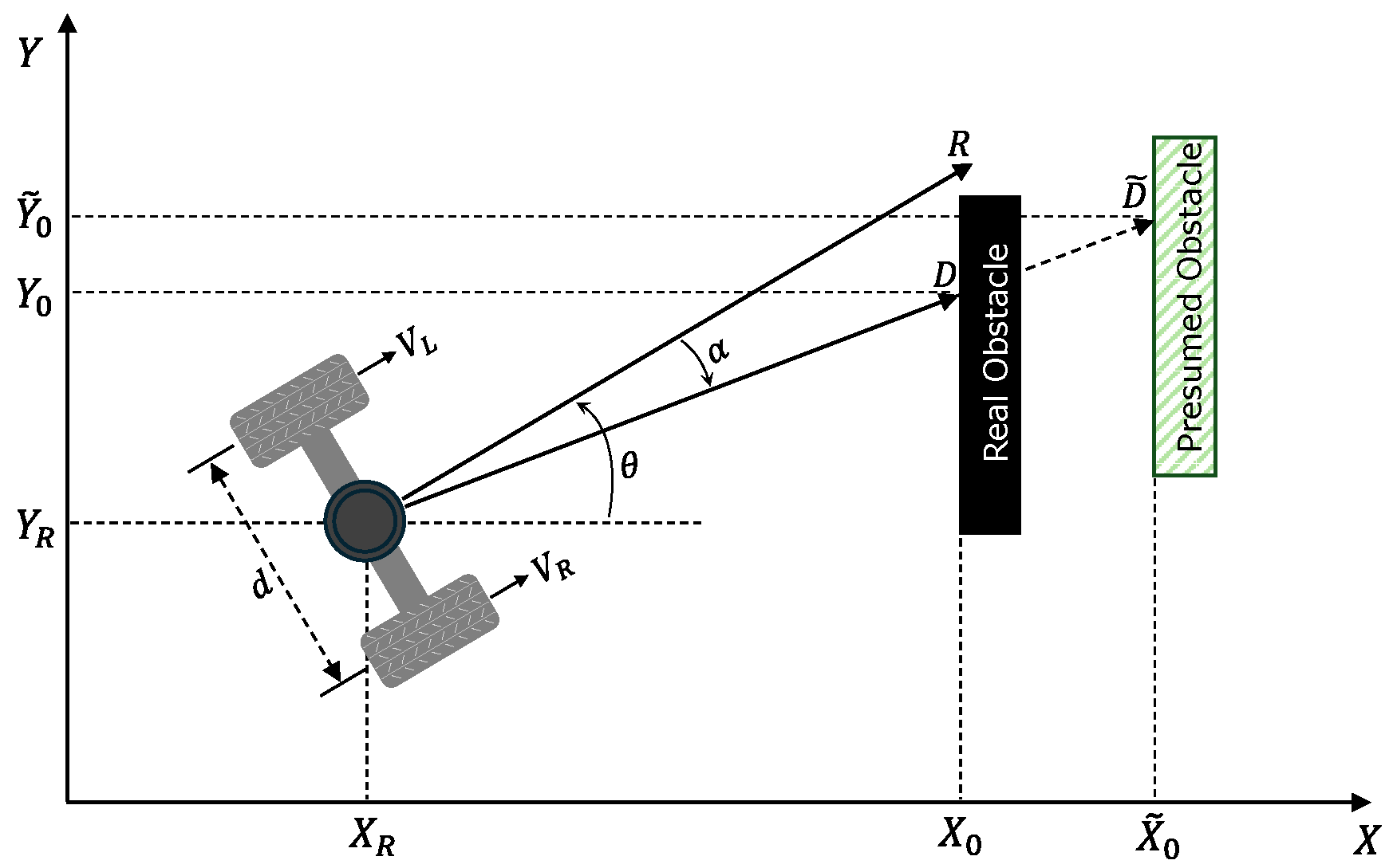
Figure 1 shows a differential single-axle planar robot, which is used throughout this paper to generate results. $V_L$(m/s) and $V_R$(m/s) are the linear speeds of the left and right wheels on the x-axis of the body-fixed frame. A difference between these two speeds lies in an inertial yaw rate on the vehicle, which is assumed to be the same as the variation of heading angle $\theta$ in the no-slip conditions.

This paper presumes that the robot can estimate its global location ${\left[X_r{Y}_r\right]}^T$ within the map using a simultaneous localisation and mapping (SLAM) algorithm.

The robot is equipped with a 2D narrow-beam light detection and ranging (LiDAR) sensor, which is located at its centre of gravity. As adjustable parameters, this sensor is assumed to emit 72 rays as per rotation, and hence the angular scanning resolution is ${\displaystyle \frac{{360}^{°}}{72}}$ or 5°. The reflected pulses are used to measure the distance of the obstacle, which is then summed up with the robot’s location to estimate the obstacle’s location. If there is no reflection, it assumes no obstacle within the nominal range R of the sensor [22].

This research employs distinct LiDAR sensor models for the HIPP and posterior problems. In the HIPP problem, the sensor model deliberately incorporates measurement uncertainties in both scan range and direction. Conversely, for the posterior problem, the sensor model generates laser scans with precise and predetermined range and directional characteristics.

Accurate mapping depends critically on how sensor uncertainty and LiDAR measurement noise are represented in the underlying map. Classical occupancy-grid mapping with forward sensor models treats range measurements as conditionally independent with Gaussian noise, updating per-cell occupancy probabilities via Bayesian filtering [28]. Experimental work with multispectral LiDAR shows that incidence angle and wavelength affect returned intensity and derived surface properties, implying scene-dependent measurement uncertainty rather than homogeneous Gaussian noise [29]. More recent formulations, therefore, incorporate explicit LiDAR and pose uncertainty into occupancy updates [23], or model map and surface uncertainty in a continuous fashion using Gaussian processes with Gaussian mixture model priors [30]. These results highlight that path-planning and exploration strategies which reason over occupancy maps built from simplistic noise assumptions may become over-confident near reflective materials, motivating explicit treatment of sensing uncertainty when designing informative planners for hazardous, cluttered domains. This research, however, uses the classical model of the LiDAR uncertainty, as the main focus is on the optimality of the path planning solution rather than the accuracy of the map.

Figure 1 shows an example measurement by an uncertain LiDAR sensor. While the location of an obstacle is measured as ${\left[X_o{Y}_o\right]}^T$, an additive white Gaussian noise (AWGN) is added to each measurement to imitate the uncertainty of the sensor:

$$\left[\begin{array}{c}\widetilde{X_o}\\ \widetilde{Y_o}\end{array}\right]=\left[\begin{array}{c}{X}_o\\ Y_o\end{array}\right]+\gamma ;\gamma \sim \mathcal{N}(\left[\begin{array}{c}0\\ 0\end{array}\right],\left[\begin{array}{cc}{\sigma }_{X{X}^2}& 0\\ 0& {\sigma }_{Y{Y}^2}\end{array}\right]).$$

(1)

where $\gamma$ is a multivariate random number with a normal distribution. The uncertainty in the X and Y directions is independent with a respective variance of ${\sigma }_{xx}$ and ${\sigma }_{yy}$. The difference between these two values is a model depicting the uncertain deflection of the rays.

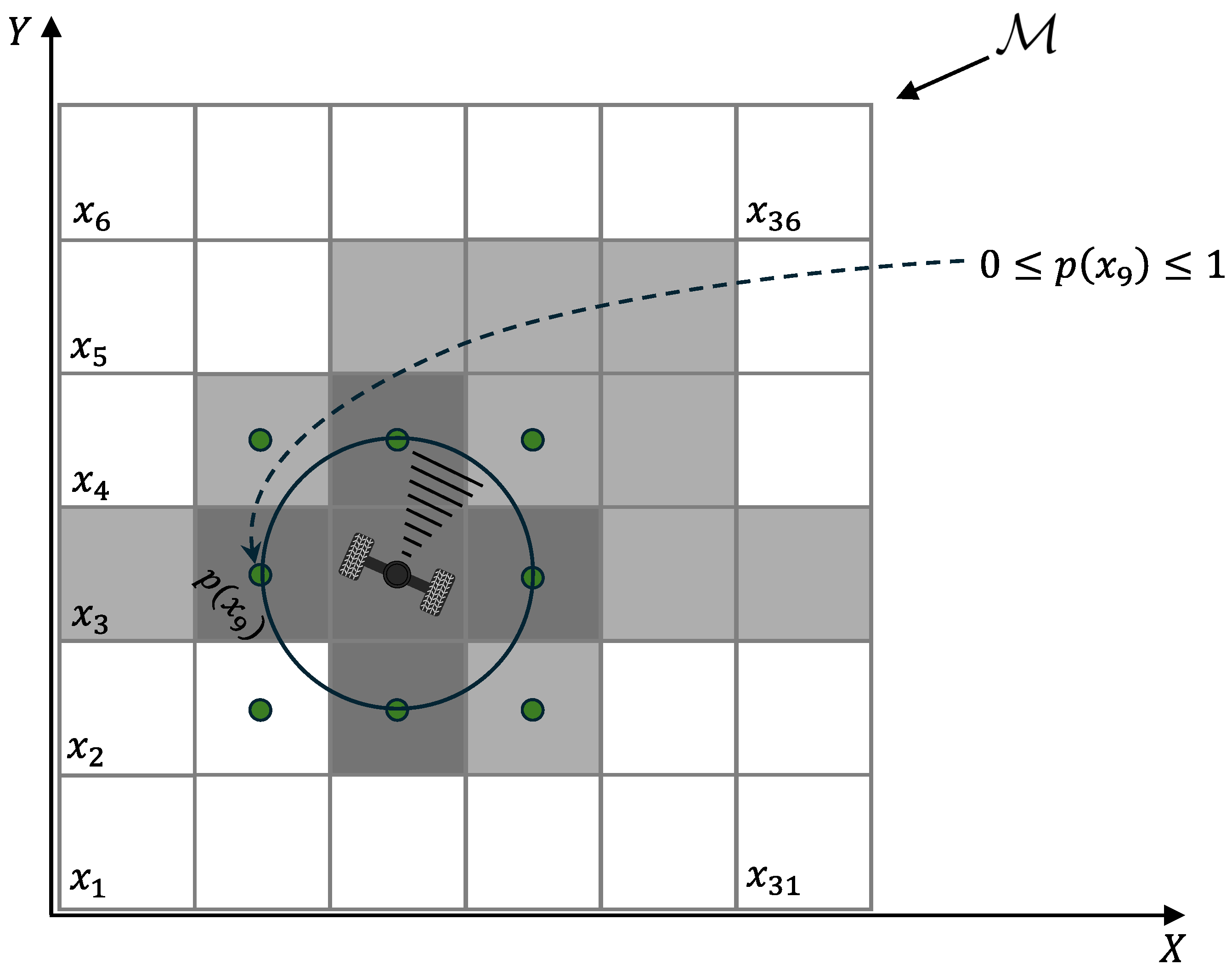
Figure 2 compares sensor measurements for the ideal and uncertain cases. The sensor model for the posterior problem represents an ideal sensor with a certain range of $1\times$ cell-width in Figure 2. A cell is considered scanned if the middle point of the cell, marked by green dots, is within the range of the sensor.

The scanned environment is depicted as an occupancy grid map (OGM) [31]. Figure 2 illustrates an example map $\mathcal{M}$ consisting of $N=36$ cells $C_j,j\in \{1..N\}$. The cells are sequentially numbered in a vertical arrangement, ascending from the bottom cell to the top cell.

Each cell in the map $\mathcal{M}$ carries an integer $n_{ray}$ indicating the number of times the sensor rays pass through that cell. In other words, $n_{ray}$ increases every time a pulsed light passes through the cells in any direction. $n_{ray}$ is capped by 72 since the cells where the robot is located, and hence known as empty, are ideally scanned 72 times when the sensor resolution is $5^{°}$. Using $n_{ray}$, a probability $P\left(C_j\right)$ is calculated for each cell as the likelihood of the cell not being empty, i.e., occupied by an obstacle. The mapping is carried out progressively, meaning that any modifications, such as moving obstacles, in previously mapped areas necessitate remapping.

3. The Proposed HIPP Algorithm

This section presents the theoretical principles and design of the proposed HIPP algorithm. It is important to note that the final destination of the robot is unspecified (as the environment is unknown), and exploration is completed when either a map with a given certainty is created or time reaches a threshold.

Algorithm 1 summarises the proposed HIPP algorithm as a pseudo-code, including four major sections: (i) generating an occupancy grid map in lines 3–5; (ii) estimating the information gain of each cell and finding the cells with the highest rewards in lines 6–7; (iii) finding the shortest paths from the current robot position passing through all the identified cells and selecting the first element of the path as the next destination, as in line 8–9; and (iv) moving the robot along this path for one sampling time considering the potential obstacles in lines 10–13. These sections are elaborated on in the following paragraphs.

Algorithm 1 A pseudo-code of the proposed HIPP algorithm

1 Initialise map $\mathcal{M}$ of arbitrary size N with $n_{ray}\left(C_j\right)=-1$ and mutual information gain $\mathcal{I}$ of the map with $i\left(C_j\right)=0$ (i.e., all cells are unknown). Initialise the initial location of robot $z_{orig}=[X_{r,0},Y_{r,0}]$. Initialise sampling time $T_s$, mission time $T_f$, map reliability threshold $p_{th}$ and $k=1$.   2 while $k<T_f/T_s$ or number of unmapped cells $\ge p_{th}$ do   3    $tmpMap$← depthScan($z_{orig}$) returns a ${360}^{°}$ sensor reading   4    $\mathcal{M}\leftarrow$ element-wise $\mathcal{M}+tmpMap$   5    $p\left(C_j\right)$← updateProbability($p\left(C_j\right)$) $\forall j\in 1..N$ using (2)   6    $\mathcal{I}$← updateInformationGain($\mathcal{I}$, {$p\left(X_0\right)..p\left(X_N\right)$}) penalising travel distance too, as in (6)   7    $cells$← highestInformation($\mathcal{I}$) using an $ϵ$-greedy algorithm to select a predefined number of cells with the highest surrounding information   8    ${\mathcal{P}}_k$← shortestPath($z_{orig}$, $cells$)   9    $z_{dest}\leftarrow {\mathcal{P}}_k\left(1\right)$ 10    if isObstacle($z_{orig}$, $z_{dest}$) then 11      $z_{dest}$← RRT*($z_{orig}$, $z_{dest}$) 12    end if 13    $z_{orig}$← moveRobot($z_{orig}$, $z_{dest}$) 14    k←$k+1$ 15 end while 16 returns $\mathcal{M}$ and $p\left(\mathcal{M}\right)$

3.1. Map Generation

The uncertain reading of a LiDAR sensor at line 3 of Algorithm 1 is used to generate ${\mathcal{M}}_k$ containing the cumulative number of rays $n_{ray}$ passing through each cell up to sampling time k. The generated map is assumed to be a stochastic 2D occupancy grid map where the robot’s belief of cell $C_j$ at each time k is implicitly calculated as

$$\begin{array}{cc}\hfill p(C_j;k)& =1-{\displaystyle \frac{min({\sum }_{l=1}^k{n}_{ray}(C_j;l),72)}{min(max\left({\mathcal{M}}_k\right),72)+ϵ}};\forall j\in 1..N.\hfill \end{array}$$

(2)

where a small positive $ϵ={10}^{-3}$ is added to prevent the singularity in numerical calculations. Also, as explained in Section 2, using a sensor with a resolution of $5^{°}$, a cell $C_j$ is considered a certainly empty cell once 72 rays have passed through it. Since the denominator of the robot’s belief in (2) is nonlinear, the iterative nature of (2) is implicit, and it is not trivial to decompose the odds ratio of the inverse sensor model.

By definition, $p\left(C_j\right)\in [0,1]$. Values close to 1 indicate either that the cell is occupied or that there is no information about its state, while $p\left(C_j\right)=0$ corresponds to a certainly free cell. For a truly free cell, $p(C_j;k\to \infty )$ converges to 0, as the numerator in (2) grows faster than the denominator until convergence. For an occupied cell, $p\left(C_j\right)$ remains close to 1, with only small variations due to measurement noise.

To clarify the impact of the proposed formulation on the reliability of the information gain estimate, the behaviour of $p\left(C_j\right)$ is examined more explicitly.

The global coupling introduced by the normalisation term does not lead to unbounded growth. The denominator saturates quickly and, after the first full LiDAR rotation, no longer increases, which limits its influence across the map. In this context, $p(C_j;k)\approx 1$ is interpreted as an unobserved or uninformed state rather than a confident occupancy estimate, as the latter is unusual due to the uncertain nature of the sensor measurements. Unobserved cells, therefore, remain close to 1 after initial exposure and only decrease as measurements accumulate, reflecting the incorporation of evidence.

Consequently, the apparent increase in occupancy probabilities for unobserved cells due to the accumulation of measurements is not an artificial inflation of information gain, but a direct result of representing unobserved space as unknown. As observations are incorporated, these values evolve consistently towards either free or occupied states, ensuring that the information gain remains driven by actual measurements rather than numerical artefacts. Consistently, the adopted information formulation assigns minimal informative value to such rarely observed cells with $p(C_j;k)\approx 1$ until sufficient LiDAR measurements are accumulated.

3.2. Approximation of Information

HIPP estimates a mapping gain for each already mapped cell, representing the potential expansion of the map if the robot moves to that cell. Having the previous travelled path ${\mathbf{Z}}_{1:k}$, this mapping gain at any time k is equivalent to the mutual information $\mathcal{I}({\mathcal{M}}_k;C_{k+1}|{\mathbf{Z}}_{1:k})$ between the map ${\mathcal{M}}_k$ and the next destination of robot $C_{k+1}$ and is defined as [15]

$$\begin{array}{cc}\hfill \mathcal{I}({\mathcal{M}}_k;C_{k+1}|{\mathbf{Z}}_{1:k})=& \mathcal{H}\left({\mathcal{M}}_k\right|\mathcal{O}\left({\mathbf{Z}}_{1:k},C_{k+1})\right)-\hfill \\ \hfill & \mathcal{H}\left({\mathcal{M}}_k\right|\mathcal{O}\left({\mathbf{Z}}_{1:k}\right))\hfill \end{array}$$

(3)

where $\mathcal{H}\left({\mathcal{M}}_k\right|\mathcal{O}\left({\mathbf{Z}}_{1:k}\right))$ is the conditional entropy of map ${\mathcal{M}}_k$ knowing the previous observation $\mathcal{O}$ over the path ${\mathbf{Z}}_{1:k}$, and $\mathcal{H}\left({\mathcal{M}}_k\right|\mathcal{O}({\mathbf{Z}}_{1:k}:C_{k+1}))$ is a similar entropy when the next step destination at time k (i.e., $C_{k+1}$) is also known.

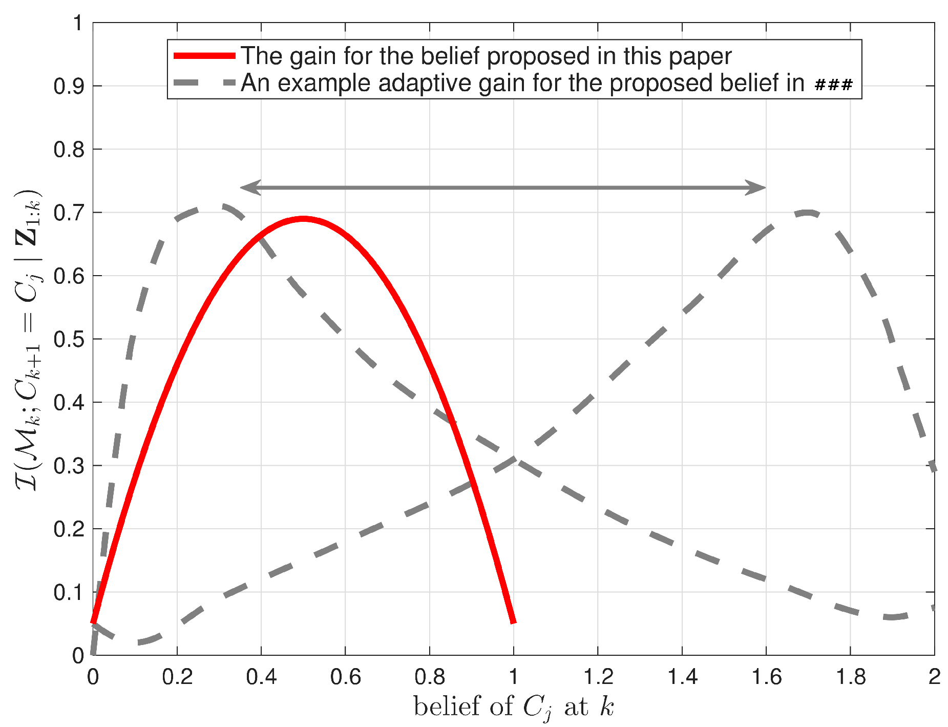
The authors in [15] formulated the belief that a cell is occupied as the odds ratio between zero and infinity. They proposed an information gain function which monotonically increases before a peak, where it switches to monotonically decrease. They also introduced a mechanism to adjust the information gain function by leaning its peak towards the low values of the belief or the other way around, as in Figure 3, depending on the guess of the next sensor reading for the cell. This helps to moderately correct an occupied belief by a new empty reading for a cell, and sharply strengthen an empty belief by a new reading which confirms the emptiness of the cell.

Conversely, this paper proposes (2) to calculate belief as a positive number less than one. This helps to apply the Shannon formula to heuristically approximate the mutual information gain at each time k between the map ${\mathcal{M}}_k$ and the new location of the robot $C_j$

$$\mathcal{I}({\mathcal{M}}_k;C_{k+1}=C_j|{\mathbf{Z}}_{1:k})\approx {\mathcal{H}}_s(C_j;k);\forall j\in \{1..N\}.$$

(4)

where the Shannon entropy ${\mathcal{H}}_s$ is as follows:

$$\begin{array}{c}\hfill {\mathcal{H}}_s(C_j;k)=-\sum _{x\in \{0,1\}}p(C_j=x;k)logp(C_j=x;k)\end{array}$$

(5)

To account for the potential information gain in the neighbourhood of cell $C_j$, the proposed algorithm applies a $3\times 3$ integration kernel to emphasise high-information regions. Obstacles within this neighbourhood are modelled via a parametric penalty that introduces a repulsive effect across spatial scales; however, this term is set to zero in the reported experiments. The travel distance is also taken into account as an additive penalty. The resulting information gain is then formulated as

$$\begin{array}{cc}\hfill & {\mathcal{I}}_f({\mathcal{M}}_k;C_{k+1}=C_j|{\mathbf{Z}}_{1:k})=\hfill \\ \hfill & [{\mathcal{I}}_f({\mathcal{M}}_k;C_{k+1}=C_j|{\mathbf{Z}}_{1:k})-\beta ∥z_{k+1}-z_k∥]\ast \left[\begin{array}{ccc}1& 1& 1\\ 1& 1& 1\\ 1& 1& 1\end{array}\right].\hfill \end{array}$$

(6)

where ∗ represents the matrix convolution operator and $\beta \in [0,1]$ is the penalising factor of direct distance. $z_{k+1}$ is the location of the cell $C_j$’s centre.

Figure 3 illustrates the resulting curve (i.e., the solid red curve) of the proposed information gain with respect to the current belief of cell $C_j$. This formulation suggests that the cells which are the most uncertain (i.e., their belief is $0.5$) receive the maximum gain if the robot moves to them.

3.3. Path Generation

If the mutual information gain (3) increases monotonically with the belief of cell $C_{k+1}$ up to a peak and then decreases monotonically thereafter (as described in Lemma 3.1 of [15]), it follows that a path planning algorithm aiming to maximise this mutual information will eventually direct the robot toward unexplored areas (see Theorem 2.5 in [15]).

Building on this theoretical foundation, this paper introduces the HIPP algorithm, which maximises $I_f$ as defined in (6). As illustrated in Figure 3, the proposed information gain function in (6) satisfies the conditions of Theorem 2.5 in [15], showing both monotonically increasing and decreasing segments. Consequently, the HIPP algorithm will eventually explore and map all previously unknown regions. In other words, the mutual information between the robot’s observations and the constructed map will asymptotically decrease, as shown in Section 5.4.

At each sampling time k, the proposed strategy selects a predefined number of cells with the highest information gain. An $ϵ$-greedy algorithm is used for this selection to add elements of exploration as well. A travelling salesperson problem with return is, then, formulated and solved to find the shortest path ${\mathcal{P}}_k$ starting from the current location of the robot and passing through all the selected cells before returning to the current location.

Robot Control and Potential Obstacle Avoidance

The proposed HIPP algorithm calculates the velocities of the left and right wheels to move the robot to the first destination of the calculated path ${\mathcal{P}}_k$ (i.e., ${\mathcal{P}}_k\left(1\right)$). The velocities are applied to the robot for a sampling time $T_s$.

HIPP examines if there is an obstacle between the current location of the robot and the desired destination ${\mathcal{P}}_k\left(1\right)$. If an obstacle is detected, RRT* is applied to find a path which avoids collision (Algorithm 2, line 8). Then, the first element of this path is considered the robot’s next destination.

Algorithm 2 A pseudo-code of the proposed solver to approximate a solution to the posterior problem (7), i.e., the benchmark solution of HIPP

1 Initialise the map $\mathcal{M}$, number of way-points $N_{wp}$, initial location of robot $z_{orig}=[X_{r,0},Y_{r,0}]$, required number of generations $N_{gen}$ and k = 1.   2 ${\mathcal{S}}_0$← randomSeedsOnMap($\mathcal{M}$, $N_{wp}$)   3 while  $k\le N_{gen}$  do   4    $\mathcal{V}\leftarrow$ createVoronoiPartitions($\mathcal{M},{\mathcal{S}}_{k-1}$)   5    for $i=1:N_{wp}$ do   6      ${\mathcal{S}}_k\left(i\right)\leftarrow$ updateWayPoints(${\mathcal{S}}_{k-1}\left(i\right)$, $\mathcal{V}$) using the modified version of the algorithm in [2], proposed in Section 4   7      if isObstacle(${\mathcal{S}}_k\left(i\right)$, ${\mathcal{S}}_{k-1}\left(i\right)$) then   8         ${\mathcal{S}}_k\left(i\right)$← RRT*(${\mathcal{S}}_{k-1}\left(i\right)$, ${\mathcal{S}}_k\left(i\right)$)   9      end if 10      ${\mathcal{S}}_k\left(i\right)$← moveRobot(${\mathcal{S}}_{k-1}\left(i\right)$, ${\mathcal{S}}_k\left(i\right)$) 11    end for    k←$k+1$ 12 end while 13 $G({\mathcal{S}}_{N_{gen}},E)\leftarrow$ generateGraph(${\mathcal{S}}_{N_{gen}}$) with the edges connecting way-points with line-of-sight by their Euclidean distance 14 if there is no connected graph then 15    increase $N_{wp}$ and run the algorithm again 16 end if 17 $\mathcal{P}\leftarrow$ shortestPath($z_{orig}$, ${\mathcal{S}}_{N_{gen}}$) calculates exhaustively the shortest path from $z_{orig}$ passes all the way-points as in Section 4 18 returns $\mathcal{P}$

4. The Proposed Algorithm to Calculate Benchmark Solution

This section develops a novel algorithm to generate a benchmark solution for the proposed HIPP. Principally, this benchmark is the optimal solution of the posterior mapping problem, where the robot finds the shortest path to remap a known environment. A formulation of the posterior problem as a minimum-time optimal control problem is provided as

$$\begin{array}{cc}& {\mathbf{U}}^{*}(z_{init},G,R)=\arg \underset{\begin{array}{c}\mathbf{U},N\end{array}}{\mathrm{maximise}}J(map,\mathbf{X},\mathbf{U}):=\hfill \end{array}$$

$$\begin{array}{cc}& {\displaystyle \sum _{k=1}^N}\left[\alpha f_I\left({\mathcal{M}}_k,u_k|{\mathbf{Z}}_{1:k}\right)-\beta f_d\left(z_k,u_k\right)\right]-\hfill \\ \hfill & \mu N+\gamma \left|{\mathcal{M}}_N\right|\hfill \\ \mathrm{where}:\hfill & \end{array}$$

(7a)

$$\begin{array}{cc}& f_I\left({\mathcal{M}}_k;u_k|{\mathbf{Z}}_{1:k}\right)=\left|{\mathcal{M}}_k\cup sur\left(u_k,R\right)\right|-\left|{\mathcal{M}}_k\right|\hfill \end{array}$$

(7b)

$$\begin{array}{cc}& f_d\left(z_k,u_k\right)={∥z_k-u_k∥}^2\hfill \\ \mathrm{s}.\mathrm{t}.:\hfill & \end{array}$$

(7c)

$$\begin{array}{cc}& {\mathcal{M}}_{k+1}={\mathcal{M}}_k\cup sur\left(u_k,R\right);{\mathcal{M}}_1=\varnothing \hfill \end{array}$$

(7d)

$$\begin{array}{cc}& z_{k+1}=u_k;z_1=z_{init}\hfill \end{array}$$

(7e)

$$\begin{array}{cc}& {\mathbf{V}}_{k+1}={\mathbf{V}}_k\cup u_k\hfill \end{array}$$

(7f)

$$\begin{array}{cc}& u_k\in {\mathbf{U}}_k\left(G\right)\setminus {\mathbf{V}}_k\hfill \end{array}$$

(7g)

where $G(\mathbf{U},\mathbf{E})$ is a graph of all feasible locations $\mathbf{U}$ of the robot on the map. Every two locations with a line-of-sight are connected by an edge $e\in \mathbf{E}$ representing their Euclidean distance. ${\mathbf{U}}_k\left(G\right)=\{u\mid u\in \mathbf{U}$; there is a direct link from $z_k$ to u in the graph G }, $V_k$ ={ $u\mid u\in U$; u is an already visited vertex up to time k}, $sur(u_k,R)$ is the set of the surrounding cells of $u_k$ with a sensor of range R. $\alpha$ and $\beta$ are arbitrary convex coefficients. $|.|$ returns the cardinality of a set.

The objective of the problem (7) implies that the control strategy must find the shortest path that maximises the size of the generated map $\mathcal{M}$ in a minimum time N. It is important to highlight that the final destination is unknown, adding complexity to the problem and contributing to its strong non-convexity. In addition, the discontinuous nature of the difference equation (7d) further complicates the numerical solution of problem (7).

This paper proposes an investigative solver to approximate a solution to the problem (7). Algorithm 2 summarises the proposed solver as a pseudo-code. As shown, the solver combines a CPP (Algorithm 2, lines 4–6) and a TSP (Algorithm 2, lines 13–17) algorithm. The CPP algorithm optimally locates a given number of way-points on the map to maximise the coverage with a given sensor range R. The TSP algorithm, then, finds the shortest path from the initial point to an unknown destination that passes all the dispersed way-points.

The CPP algorithm randomly seeds a finite number of way-points across a map. Then, it creates Voronoi partitions [32,33] for the seeds based on a range-limited visibility disc proximity measure [21], thereby decomposing the coverage problem among the way-points.

The free-arc method from [32] calculates the vector of movement of the way-points in a non-convex environment. After creating Voronoi partitions, the method draws a circle around the way-points with a radius of the sensor range R. Parts of the circle’s edge outside of the Voronoi partition of the way-point are discarded and only the parts inside the partition are used to calculate the velocity (speed and direction) of movement of the way-points. Specifically, the movement vector $k\widehat{m}$ of the way-point is the vector sum of the resulting velocity $k_j{\widehat{m}}_j$ of each arc j. The velocity due to each arc is calculated by splitting the arc into segments with an equal length of $dq$ and a centre point of $p_i$. Therefore, the velocity of the required movement of a way-point is calculated as

$$k\widehat{m}={\displaystyle \sum _{j=1}^{N_{arcs}}}{\int }_{p_i\in ar{c}_j}\varphi \widehat{n_i}dq$$

(8)

where $N_{arcs}$ is the number of eligible arcs, ${\widehat{n}}_i$ is the unit normal vector to the segment with the centre $p_i$, $dq$ is the length of segments and $\varphi$ is a gain indicating the importance of each segment (that can be one for all segments). In other words, each segment $p_i$ affects the way-point velocity by a factor $\varphi dq$ in the direction of $\widehat{n_i}$. For more details, refer to the works of authors in [32].

The optimally relocated way-points by the free-arc algorithm create a graph connecting only those points with unobstructed line-of-sight paths. By solving a travelling salesman problem (TSP) for each vertex of the graph [34], the method determines the shortest route that starts from the robot’s original location and traverses all way-points, effectively providing a close-to-optimal solution for the problem (7).

Readers are referred to [35] for further clarification.

5. Results and Discussions

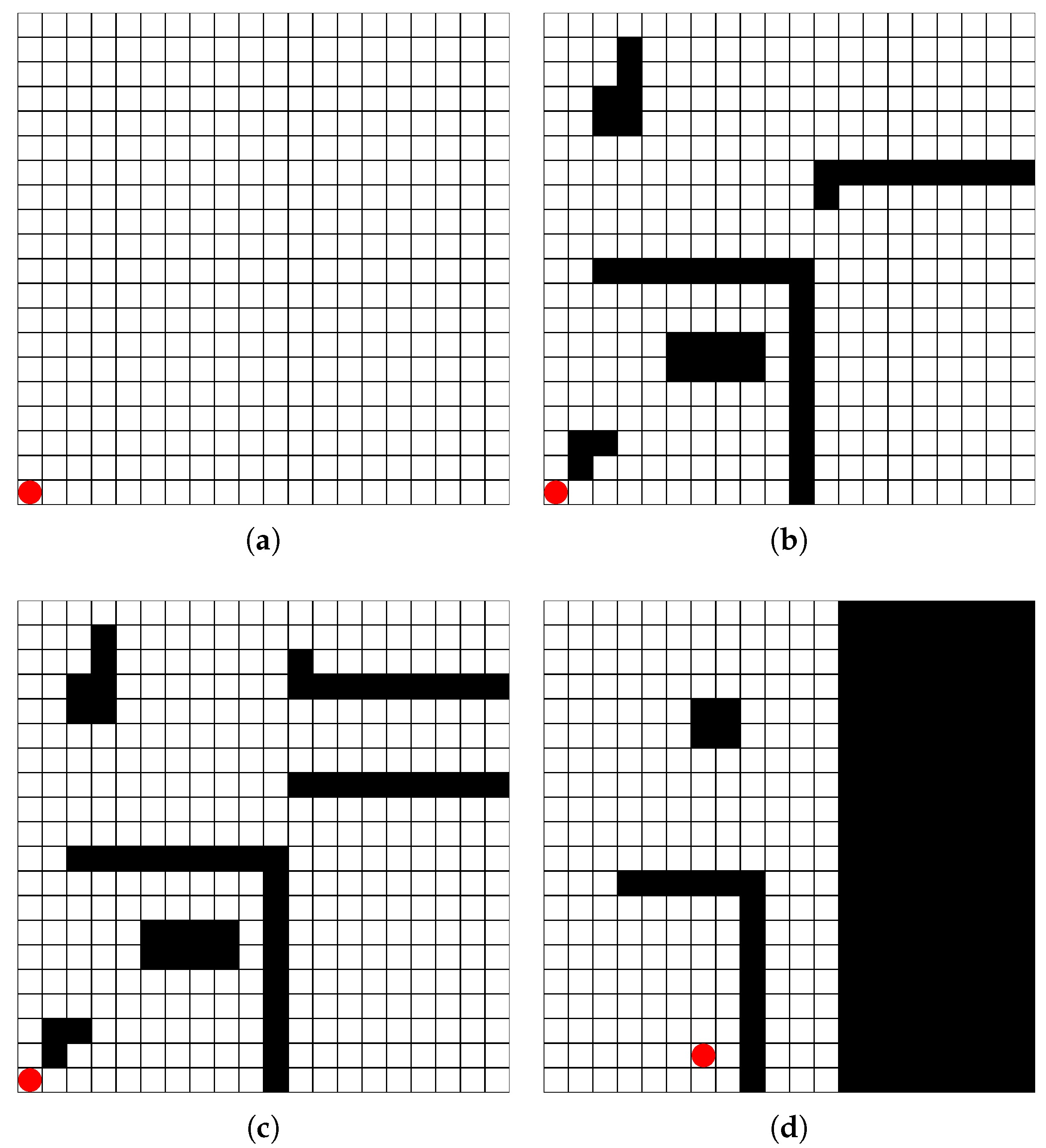
The four maps in Figure 4 are used as Test Scenarios 1 to 4 to evaluate the adaptation and efficacy of the proposed HIPP algorithm to different environments.

Table 2. Hyperparameters used in the proposed exploration and obstacle avoidance framework.

Parameter	Value
Sampling time $T_s$	1 s
Track length d	0.2 m
Max velocity $v_{max}$	1 m/s
Map size	$10\times 10$ m
Grid resolution $N_{grid}$	$20\times 20$
Cell size	0.5 m
Sensor range	1.5 cells
Standard deviation of the sensor noise ${\sigma }_{XX}={\sigma }_{YY}$	0.25 m
Success threshold of the solver $p_{th}$	$5\%\times N_{grid}$
Scan resolution	$5^{°}$
Penalising factor of direct distance $\beta$	$0.02$
RRT* Max iterations	100
RRT* Goal bias	0.5 m
RRT* Step size	1.5 m
RRT* Rewiring factor	2 m
Final time $T_f$	200 s
Number of points in Algorithm 2 $N_{wp}$	100

lists the hyperparameter values used for the robots and simulations. The standard deviation sensor noise is intentionally set to an order of magnitude higher than the nominal specification to emulate adverse environmental conditions and evaluate the robustness of the proposed method.

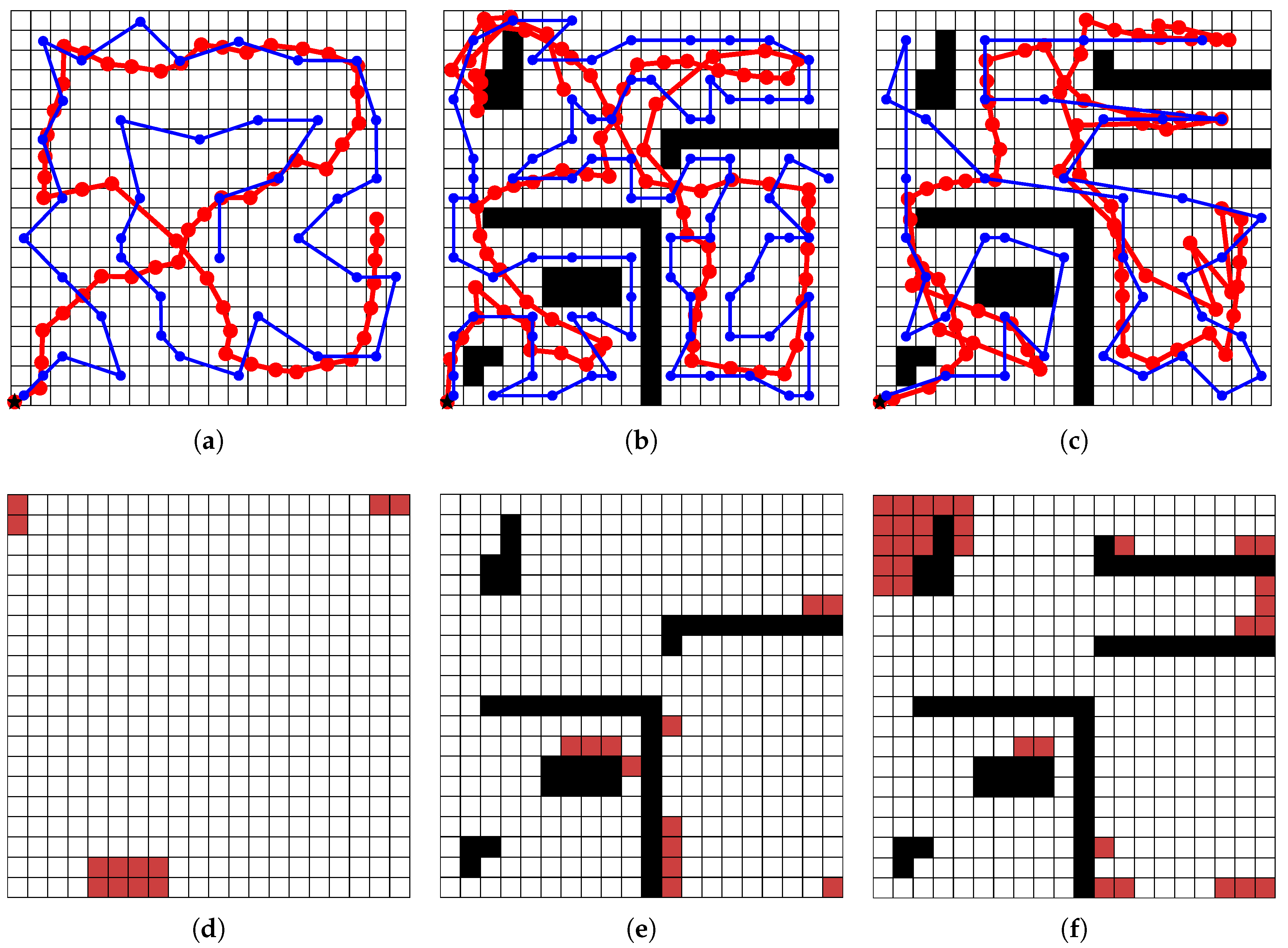
Figure 4a is an empty map, whilst Figure 4b is a complex map with multiple rooms and obstacles. Figure 4c, as compared to Figure 4b, consists of a narrow dead-end passage. Figure 4d illustrates the real-world setup used to empirically validate the performance of the developed algorithm in Section 5.2. The results and performance of the proposed HIPP algorithm are evaluated and benchmarked against the solutions to the proposed posterior problem. Without loss of generality, the initial position of the robot in all scenarios is assumed identical, as the red circles in the left-bottom corner of Figure 4.

The comparison measure is the number of identified cells on the OGM map normalised by the travel distance. However, to make a fair comparison, an equivalent number of identified cells is introduced, which is the number of identified cells calculated by placing the ideal sensor of Figure 2 at the generated way-points by HIPP. Hence, a realistic comparison measure is the equivalent number of identified cells per unit of travel distance.

Moreover, this section provides an optimality analysis where the cumulative performance of the proposed HIPP over the travelling time is benchmarked against the solution of the proposed posterior problem. In other words, it shows whether the number of identified cells increases linearly with the travelling time.

The confidence of the mapped cells is measured by the number of times a cell is sensed. This paper only considers a cell empty if the probability of being sensed as empty is equal to or more than $20\%$. It means that a cell must be scanned at least 14 times as an empty cell to be considered so.

5.1. Simulation Results

The HIPP and solver of the posterior problem have been run ten times for each test scenario.

Table 3. The statistics of total travel distance (TTD), number of identified cells ($N_{IC}$) and that per each unit of travel distance (TD) for ten runs of Algorithms 1 and 2 for Test Scenarios 1 to 3. An equivalent number of identified cells, calculated by placing the ideal sensor of Figure 2 at the generated way-points by HIPP, provides a fair comparison, as explained in Section 5.

		TTD (m)	${\mathit{N}}_{\mathit{IC}}$ (cells)	${\mathit{N}}_{\mathit{IC}}$/TD (cells/m)	Equivalent ${\mathit{N}}_{\mathit{IC}}$ (cells)	Equivalent ${\mathit{N}}_{\mathit{IC}}$/TD (cells/m)
Test Scenario 1	Algorithm 1 (HIPP) results
	Average	48.9	384.5	8.1	233.5	4.9
	Std. Deviation	12.21	13.6	2.4	15.8	1.1
	Median	49.3	388.0	7.7	231.0	4.7
	Algorithm 2 (Posterior) results,
	i.e., a benchmark solution
	Average	58.1	362.0	6.2	-	-
	Std. Deviation	1.0	6.4	0.1	-	-
	Median	58.4	364.0	6.2	-	-
Test Scenario 2	Algorithm 1 (HIPP) results
	Average	78.8	340.0	4.4	262.0	3.4
	Std. Deviation	8.8	7.4	0.6	10.0	0.4
	Median	80.6	343.0	4.3	262.0	3.3
	Algorithm 2 (Posterior) results,
	i.e., a benchmark solution
	Average	83.8	353.0	4.2	-	-
	Std. Deviation	2.9	1.7	0.1	-	-
	Median	84.4	354.0	4.2	-	-
Test Scenario 3	Algorithm 1 (HIPP) results
	Average	80.7	305.5	3.8	241.0	3.0
	Std. Deviation	7.6	27.2	0.6	18.7	0.4
	Median	80.0	313.5	3.9	244.0	3.1
	Algorithm 2 (Posterior) results,
	i.e., a benchmark solution
	Average	72.5	311.6	4.3	-	-
	Std. Deviation	2.8	8.7	0.2	-	-
	Median	72.7	310.0	4.3	-	-

summarises the statistics of the resulting total travelling time (TTD), the number of mapped cells, the number of identified cells per unit of travel distance (TD), the equivalent number of mapped cells, and the equivalent number of mapped cells per unit of travel distance (TD). As explained before, the normalised equivalent number of identified cells (i.e., the latter column of the table) by HIPP is compared to the benchmark solution.

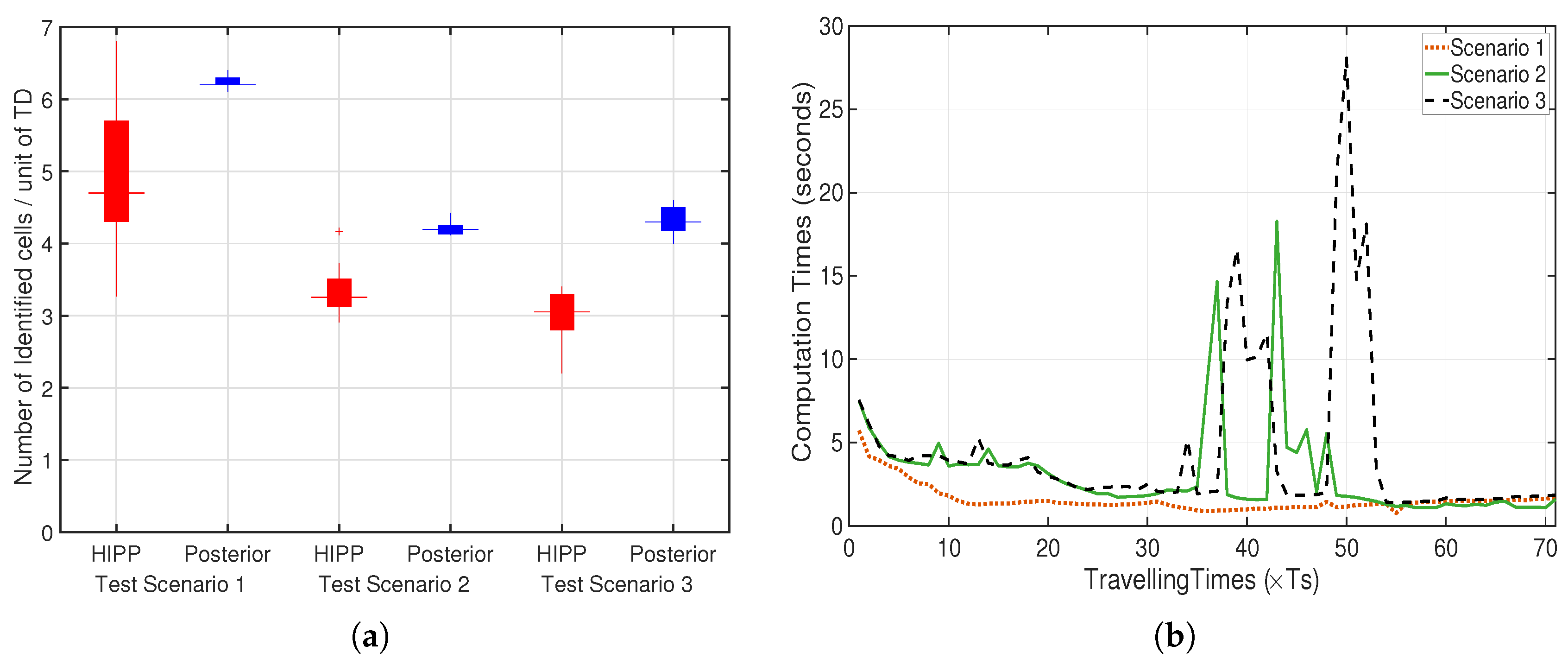
Figure 5a visualises this comparison as box plots. As shown, the average performance of the proposed HIPP reaches $72\%$ and $79\%$ of the proposed benchmark for Test Scenarios 1 or 2 and the more complex Test Scenario 3, respectively. It is worth noting that HIPP outperformed the posterior solution on one occasion in test Scenario 1, due to an empty map and an uncertain sensor. The results also show consistency in HIPP results, where the number of mapped cells per travel distance decreases as the complexity of test scenarios increases.

Figure 5b illustrates the evolution of computational time over the travel horizon for Scenarios 1–3. After the initial sampling steps, performance improves as MATLAB 2023b’s multiprocessing stabilises the computational pipeline, thereafter remains largely insensitive to map expansion. In Scenario 1, computational time shows a slight upward trend with map growth, whereas in Scenarios 2 and 3 it decreases towards the end as obstacle detection becomes less dominant. Noticeable spikes at sampling steps 36 and 42 coincide with the activation of RRT* for obstacle-free path planning. Overall, map expansion does not significantly degrade computational performance, although further optimisation is required for real-time deployment.

Figure 6 compares the best-generated paths (out of ten runs) by the proposed HIPP algorithm and the posterior problem solver. The resulting maps by HIPP are also illustrated in Figure 6d–f, indicating the unmapped parts with red cells. The readers are also referred to a prepared video (https://youtu.be/wnBgTZxwG_o, accessed on 4 May 2026) where the performance of HIPP for all three test scenarios is demonstrated.

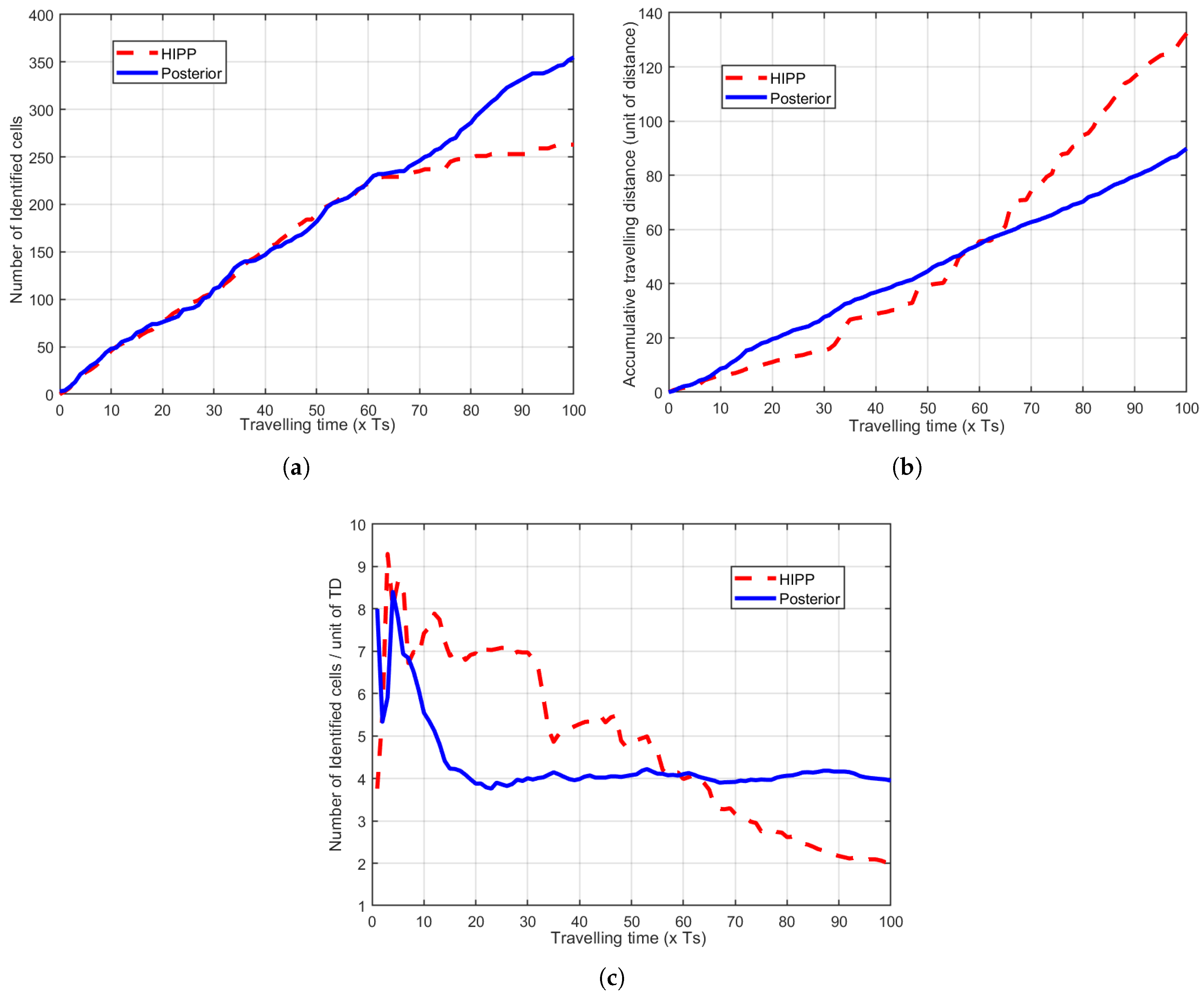
The instantaneous behaviour of the proposed HIPP algorithm over the travelling time is compared in Figure 7 to such results of the benchmark solution. These results are for Test Scenario 2; however, the other scenarios follow a similar trend.

As shown in Figure 7a, the cumulative number of identified cells by HIPP follows an almost linear increase by travelling time before it starts being saturated at around 60 sampling times $T_s$. In other words, HIPP follows the performance of the benchmark solution over a wide range of operating times before being outperformed.

However, it is shown in Figure 7b that within the same period of 60 sampling times, the robot travels less by HIPP than the benchmark solution. This means that over the first half of the travelling time, HIPP outperforms the benchmark solution in terms of the normalised identified cells by travel distance. Figure 7c illustrates this comparison measure clearly, where the number of identified cells per unit of travel distance is plotted against the travelling time. This means that HIPP implicitly prioritises the wider areas where the mapping gains are higher than in narrow passages.

Moreover, it is observed in Figure 7c that there is a sharp rise in the number of identified cells per travel distance by the solution of the posterior problem before reaching a saturated state after around 15 sampling times. This is due to scanning multiple cells with a small movement. The saturated 4 cells per unit of travel distance match the range of the sensor, which is $1.5$ cells, indicating a near-to-global optimal solution. The HIPP’s normalised number of identified cells, on the other hand, continuously decreases over travelling time before reaching 2 cells per unit of travel distance at the end of the test scenario.

5.2. Experimental Results

The performance of HIPP is empirically evaluated using a differential single-axle planar robot, the JetBot Pro AI kit (Waveshare, Shenzhen, China, https://www.waveshare.com/jetbot-ros-ai-kit.htm, accessed on 4 May 2026). The robot is equipped with an NVIDIA Jetson Nano processing board, and the RPLIDAR A1 LiDAR sensor for environmental scanning.

The experimental validation was conducted using RobiL, a Robot-in-the-Loop Simulator developed in SVeCLab at the University of Sussex for testing distributed and collaborative algorithms. RobiL provides an ROS-based (ROS1 Noetic) integrated environment that closely approximates real-world conditions while maintaining cost-effectiveness and experimental control.

The RobiL architecture comprises four essential components: a user server, a core server, a Matlab ROS Slave Server, and a visualiser server, working collaboratively to simulate and analyse robot behaviour in real time. The Matlab ROS Slave Server, hosting HIPP, operates on an Intel® Core™ i7-6700 CPU @ 3.40 GHz and Nvidia Quadro K2200 GPU, running Ubuntu 20.04. The resulting commands are transmitted to the robot through a dedicated ROS network, enabling real-time communication and seamless execution of the motion planning algorithm. To ensure practicality, the experimental map was scaled to accommodate the available laboratory space and the physical dimensions of the robot.

The HIPP’s performance is empirically evaluated by running Test Scenario 4 in Figure 4d. This scenario includes an empty room, a living room with a table, and a corridor. The robot’s RPLiDAR sensor generates 1146 samples per 360° scan, significantly surpassing the 72 samples of the simulation system. This increase means that at least 230 beams must scan a cell to raise the probability of being classified as empty to $20\%$.

Two distinct test scenarios were recorded to showcase the system’s adaptability to different Lidar range configurations during Test Scenario 4. The first video (https://youtu.be/WgJC4MoYX7w, accessed on 4 May 2026) captures the system’s performance with a Lidar range of 0.5 m, challenging the robots to navigate and respond to their environment with significantly limited sensing distance. In contrast, the second video (https://youtu.be/G88DoH2GAgQ, accessed on 4 May 2026) demonstrates the system’s behaviour with a Lidar range setting of 1.5 m, allowing for early object detection and extended environmental awareness. These experimental videos illustrate the system’s robust performance across different sensing configurations.

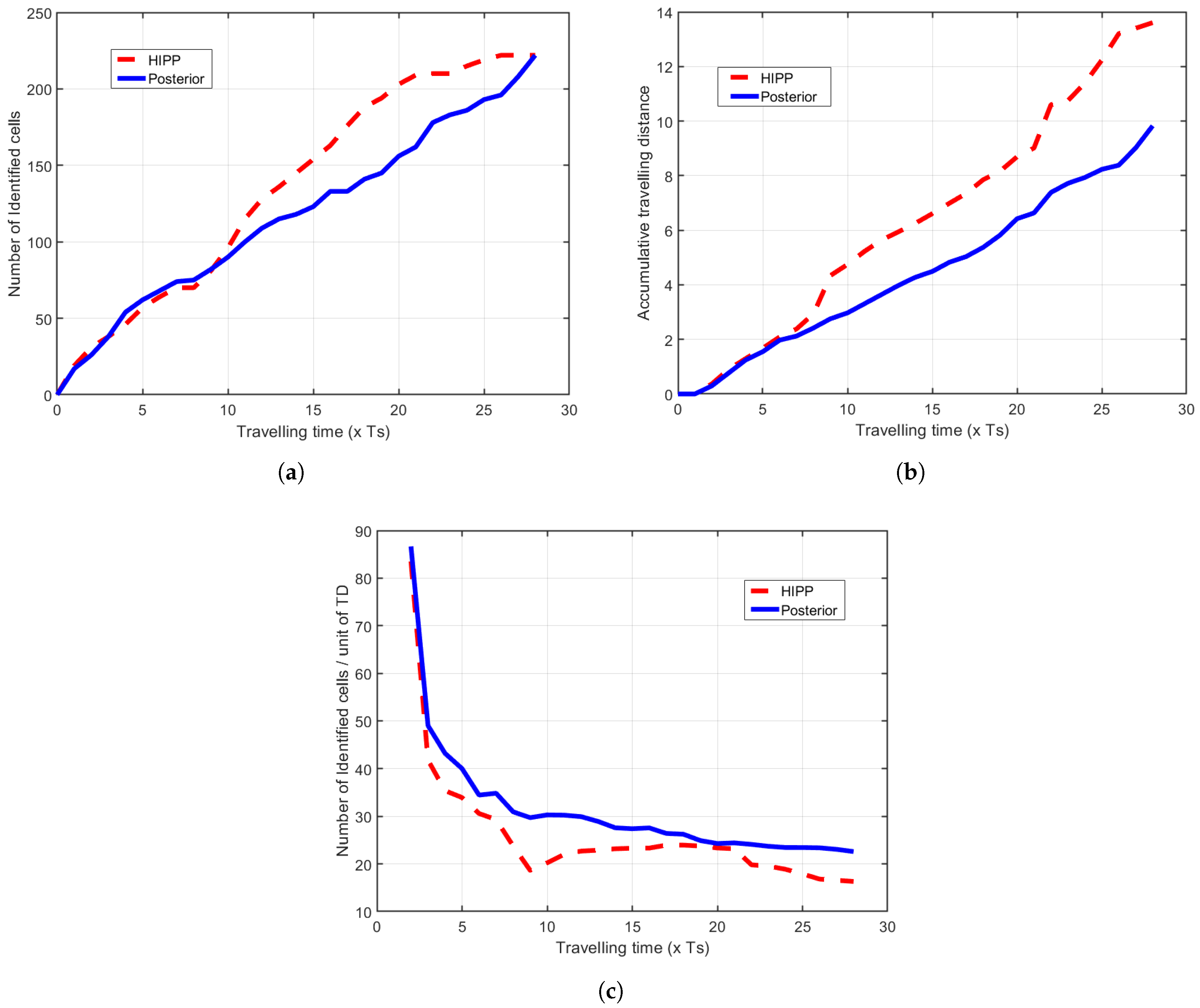
Figure 8 compares the HIPP’s performance with the benchmark solution for Test Scenario 4. As shown in Figure 8a, HIPP initially follows the benchmark solution in terms of the map expansion rate. However, after about eight sampling times, HIPP starts outperforming the benchmark solution, due to the rapid move of the robot towards unexplored areas of the map around the ninth sampling time (as in Figure 8b), which sharply increases the number of identified cells. The map expansion by HIPP is then saturated after twenty sampling times, leading to the same final number of identified cells as the benchmark solution.

Figure 8c extends such an analogy between the HIPP results and the benchmark solution by comparing the cumulative number of identified cells normalised by the travel distance. As shown, HIPP follows the benchmark solution closely except on two occasions: (i) around the eighth sampling time, when the robot travels a long distance with a high speed to get out of the small room, and (ii) the part leading to the end of the trajectory, where the robot again travels a long distance to go back and map the remaining cells in the middle of the environment.

5.3. Sensitivity Analysis to Varying Initial Position of Robot

This subsection examines the robot’s sensitivity to different starting positions across the three test scenarios in Figure 4a–c. In each test scenario, the robot is located in six carefully selected locations on maps (referred to as $z_{orig}$ in Algorithms 1 and 2). For example, some points are located in open areas while others are placed behind obstacles or within narrow corridors.

Table 4. Variations in the HIPP’s results after running three test scenarios for six different initial points indicate the algorithm’s notable robustness. Abbreviations are explained in the caption of Table 3.

	No. of Initial Point	${\mathit{N}}_{\mathit{IC}}$ (cells)	${\mathit{N}}_{\mathit{IC}}$/TD (cells/m)	${\mathit{N}}_{\mathit{IC}}$ (Benchmark)	${\mathit{N}}_{\mathit{IC}}$/TD (cells/m) (Benchmark)
Test Scenario 1	1	209	3.87	400	4.57
	2	211	3.64	400	4.65
	3	229	2.69	400	4.47
	4	242	3.59	399	4.40
	5	225	0.67	400	4.44
	6	201	0.62	400	4.47
	Average	219.5	2.35	399.83	4.50
	Std. Deviation	15.18	1.41	0.41	0.09
Test Scenario 2	1	263	1.99	355	3.95
	2	263	1.99	355	3.92
	3	263	1.99	355	3.81
	4	262	2.03	355	3.95
	5	241	1.89	354	3.81
	6	244	1.68	352	3.80
	Average	258.7	1.92	354.33	3.87
	Std. Deviation	7.33	0.13	0.82	0.07
Test Scenario 3	1	262	2.17	345	3.46
	2	257	1.79	344	3.62
	3	259	2.00	344	3.60
	4	282	2.21	346	3.47
	5	253	2.13	346	3.67
	6	256	2.16	345	3.67
	Average	261.5	2.08	345	3.58
	Std. Deviation	10.48	0.16	0.89	0.09

summarises the variation in the HIPP’s results after running three test scenarios for six different initial points as compared to the benchmark solutions. The average and the standard deviation are calculated to identify if the result may vary significantly by placing the robot in a particular position. The results in columns one and three of the table do not suggest a significant sensitivity of the proposed HIPP and benchmark solutions to changes in the initial point. The results in columns two and four of the table compare the two algorithms’ efficiency in terms of the number of cells mapped per exploration distance. The data indicates that HIPP is less sensitive to changes in the robot’s initial point in more complex scenarios. This makes sense due to the availability of fewer manoeuvre options in complex layouts.

Further analysis is provided by calculating the average deviation of the HIPP’s solution from the benchmark solution over the travel distance of each exploration (i.e., per each initial point)

$$\overline{e}={\displaystyle \frac{\parallel {\mathbf{n}}^{\mathbf{posterior}}-{\mathbf{n}}^{\mathbf{HIPP}}{\parallel }_1}{N}}$$

(9)

where ${\mathbf{n}}^{\mathbf{posterior}}$ and ${\mathbf{n}}^{\mathbf{HIPP}}$ are vectors of the accumulated number of identified cells per one exploration by the posterior and HIPP algorithms, respectively. ${\parallel .\parallel }_1$ is norm 1, which is the sum of the absolute values of the vector elements. N is the total number of sampling times over the travel distance.

Moreover, the final difference between the number of identified cells by the HIPP and benchmark solutions is calculated as a secondary error measure of the HIPP algorithm per one exploration

$$e_{end}=n_{end}^{posterior}-n_{end}^{HIPP}$$

(10)

where $n_{end}^{posterior}$ and $n_{end}^{posterior}$ are the final number of identified cells by the HIPP and posterior solutions, respectively, at the end of the exploration.

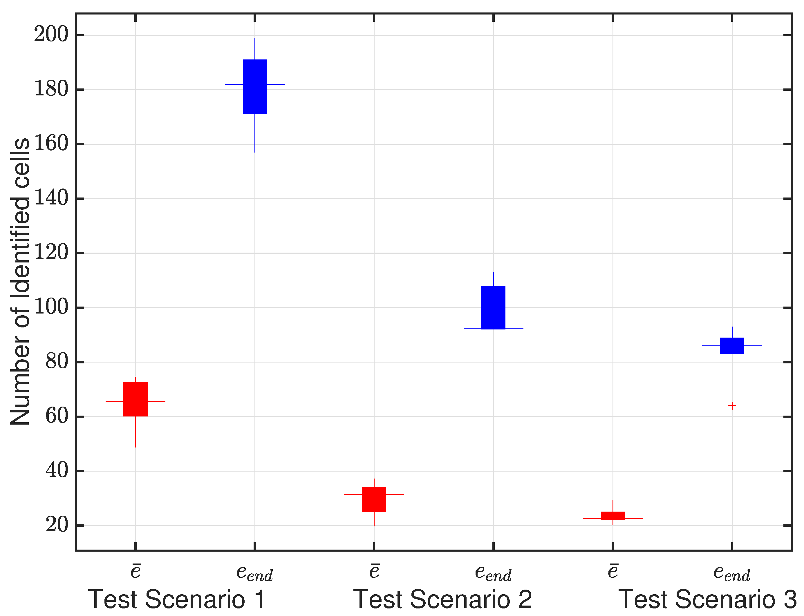
The box diagram in Figure 9 presents the calculated values of $\overline{e}$ and $e_{end}$ for each exploration of different test scenarios. It is noted that the values of these errors and their standard deviations, and hence the sensitivity of the algorithms, consistently reduce as the complexity increases in the test scenarios. This behaviour highlights HIPP’s robustness in real-world applications, where environmental complexity can enhance its mapping efficiency.

5.4. Optimality and Convergence

As depicted in Figure 7a, the benchmark solution, as detailed in Section 4, incrementally maps the area linearly until all 354 empty cells are covered. This indicates that the benchmark solution maintains a consistent performance throughout the traversal process. Its optimality is assessed by determining whether this consistent performance achieves the best possible outcome given the constraints of sensor range and the robot’s maximum permissible speed.

The theoretical upper limit of efficiency, considering a maximum sensor range of one and a half cells and a top speed of two cells per sampling time, is six detectable cells per sampling time—assuming no interference from boundaries or revisits due to cornering. The maximum traversal speed is also defined as two cell lengths (one metre) per sampling time. Additionally, the maximum traversal speed is defined as two cell lengths (equivalent to one metre) per sampling time.

As illustrated in Figure 7, the robot’s average travel speed reaches approximately 0.9 m per sampling time, with an identification rate of 3.5 cells per sampling time. This corresponds to roughly 60% of the theoretical maximum performance (3.5 cells compared to the ideal 6 cells). The discrepancy arises from revisits caused by cornering and the exclusion of out-of-bound cells near obstacles and boundaries from the total count.

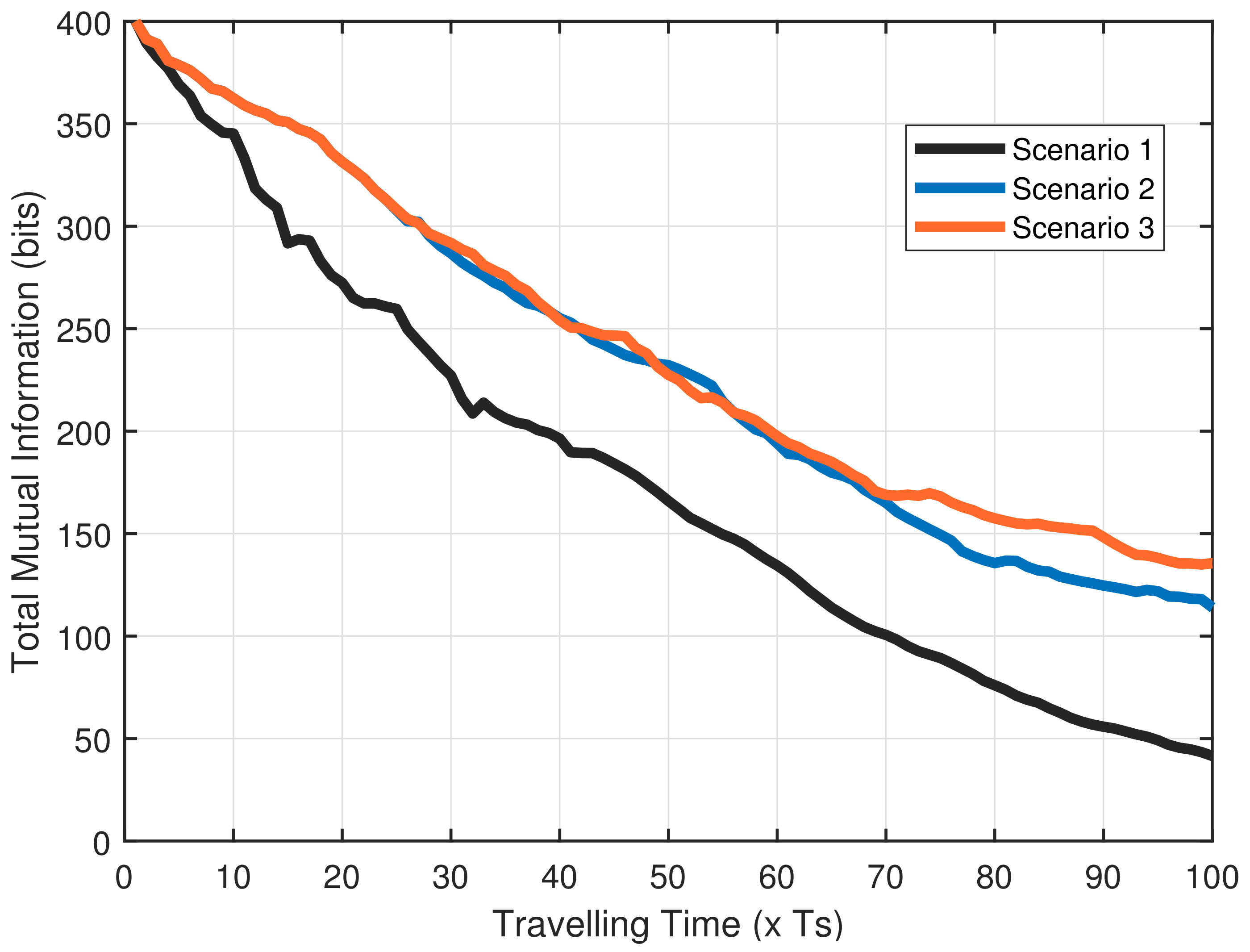
Furthermore, Figure 10 demonstrates the variation in the total mutual information over the first 100 sampling times. As shown, the developed HIPP algorithm continuously decreases total mutual information across Scenarios 1, 2, and 3. This declining pattern confirms the convergence of the proposed algorithm, aligning with the expectations established in Section 3.3.

6. Conclusions

This paper presents a novel algorithm (called HIPP) for efficiently planning a robot’s exploration path to map an unknown non-convex environment. The robot is equipped with an uncertain LiDAR sensor and the SLAM algorithm; however, it does not have prior knowledge about the environment and its final destination. The algorithm’s efficiency is measured by the number of identified cells per unit of travel distance.

A posterior problem (i.e., where the robot remaps a known map) is formulated, and its solution is considered the benchmark to evaluate the performance of the developed HIPP. It is observed that the posterior problem has potentially multiple sub-optimal solutions, making it non-trivial to solve directly. However, this paper proposes a novel algorithm to approximate the solution of the posterior problem.

The simulation and empirical results demonstrate that the proposed HIPP algorithm achieves 70–80% of the benchmark solution’s cell identification efficiency, matching its linear expansion rate while substantially reducing travel distance during initial exploration. This indicates an implicit prioritisation strategy that enables rapid mapping of the main features of the environment, a crucial advantage for navigating hazardous or complex environments.

A sensitivity analysis demonstrates the robustness of the algorithm to variations in the initial point. Both simulation and experimental results further confirm consistent operation and exploration performance across different initial conditions and scenario layouts.

HIPP demonstrates the potential for extension to swarm systems, where multiple robots collaborate to map unknown 3D environments more efficiently. Future developments in this direction would broaden the algorithm’s applicability to a wider range of real-world scenarios while preserving its benefits in travel distance optimisation and early map coverage.

References

1. Patle, B.; Babu, L.G.; Pandey, A.; Parhi, D.; Jagadeesh, A. A review: On path planning strategies for navigation of mobile robot. Def. Technol. 2019, 15, 582–606. [Google Scholar] [CrossRef] [Scilit]
2. Thanou, M.; Stergiopoulos, Y.; Tzes, A. Distributed coverage using geodesic metric for non-convex environments. In Proceedings of the 2013 IEEE International Conference on Robotics and Automation, Karlsruhe, Germany, 6–10 May 2013; IEEE: Piscataway, NJ, USA, 2013; pp. 933–938. [Google Scholar]
3. Popović, M.; Ott, J.; Rückin, J.; Kochenderfer, M.J. Learning-based methods for adaptive informative path planning. Robot. Auton. Syst. 2024, 179, 104727. [Google Scholar] [CrossRef] [Scilit]
4. Aggarwal, S.; Kumar, N. Path planning techniques for unmanned aerial vehicles: A review, solutions, and challenges. Comput. Commun. 2020, 149, 270–299. [Google Scholar] [CrossRef] [Scilit]
5. Liu, L.; Wang, X.; Yang, X.; Liu, H.; Li, J.; Wang, P. Path planning techniques for mobile robots: Review and prospect. Expert Syst. Appl. 2023, 227, 120254. [Google Scholar] [CrossRef] [Scilit]
6. Collins, L.; Ghassemi, P.; Esfahani, E.T.; Doermann, D.; Dantu, K.; Chowdhury, S. Scalable Coverage Path Planning of Multi-Robot Teams for Monitoring Non-Convex Areas. In Proceedings of the 2021 IEEE International Conference on Robotics and Automation (ICRA), Xi’an, China, 30 May–5 June 2021; pp. 7393–7399. [Google Scholar]
7. Karaman, S.; Frazzoli, E. Sampling-based algorithms for optimal motion planning. Int. J. Robot. Res. 2011, 30, 846–894. [Google Scholar] [CrossRef] [Scilit]
8. Galceran, E.; Carreras, M. A survey on coverage path planning for robotics. Robot. Auton. Syst. 2013, 61, 1258–1276. [Google Scholar] [CrossRef] [Scilit]
9. Fevgas, G.; Lagkas, T.; Argyriou, V.; Sarigiannidis, P. Coverage path planning methods focusing on energy efficient and cooperative strategies for unmanned aerial vehicles. Sensors 2022, 22, 1235. [Google Scholar] [CrossRef] [Scilit]
10. Arkin, E.M.; Hassin, R. Approximation algorithms for the geometric covering salesman problem. Discret. Appl. Math. 1994, 55, 197–218. [Google Scholar] [CrossRef] [Scilit]
11. Juliá, M.; Gil, A.; Reinoso, O. A comparison of path planning strategies for autonomous exploration and mapping of unknown environments. Auton. Robot. 2012, 33, 427–444. [Google Scholar] [CrossRef] [Scilit]
12. Muralidharan, A.; Mostofi, Y. Path planning for minimizing the expected cost until success. IEEE Trans. Robot. 2019, 35, 466–481. [Google Scholar] [CrossRef]
13. Dutta, A.; Bhattacharya, A.; Kreidl, O.P.; Ghosh, A.; Dasgupta, P. Multi-robot informative path planning in unknown environments through continuous region partitioning. Int. J. Adv. Robot. Syst. 2020, 17, 1729881420970461. [Google Scholar] [CrossRef] [Scilit]
14. Popović, M.; Vidal-Calleja, T.; Hitz, G.; Chung, J.J.; Sa, I.; Siegwart, R.; Nieto, J. An Informative Path Planning Framework for UAV-Based Terrain Monitoring. Auton. Robots 2020, 44, 889–911. [Google Scholar] [CrossRef] [Scilit]
15. Julian, B.J.; Karaman, S.; Rus, D. On mutual information-based control of range sensing robots for mapping applications. Int. J. Robot. Res. 2014, 33, 1375–1392. [Google Scholar] [CrossRef] [Scilit]
16. Charrow, B.; Liu, S.; Kumar, V.; Michael, N. Information-Theoretic Mapping Using Cauchy-Schwarz Quadratic Mutual Information. In Proceedings of the International Conference on Robotics and Automation (ICRA), Seattle, WA, USA, 26–30 May 2015. [Google Scholar]
17. Schmid, L.; Pantic, M.; Khanna, R.; Ott, L.; Siegwart, R.; Nieto, J. An efficient sampling-based method for online informative path planning in unknown environments. IEEE Robot. Autom. Lett. 2020, 5, 1500–1507. [Google Scholar] [CrossRef] [Scilit]
18. Chen, L.; Shan, Y.; Tian, W.; Li, B.; Cao, D. A Fast and Efficient Double-Tree RRT*-Like Sampling-Based Planner Applying on Mobile Robotic Systems. IEEE/ASME Trans. Mechatron. 2018, 23, 2568–2578. [Google Scholar] [CrossRef] [Scilit]
19. Jiang, J.; Wu, K. Cooperative Pathfinding Based on Memory-Efficient Multi-Agent RRT*. IEEE Access 2020, 8, 168743–168750. [Google Scholar] [CrossRef] [Scilit]
20. Huang, J.; Zhou, B.; Fan, Z.; Zhu, Y.; Jie, Y.; Li, L.; Cheng, H. FAEL: Fast autonomous exploration for large-scale environments with a mobile robot. IEEE Robot. Autom. Lett. 2023, 8, 1667–1674. [Google Scholar] [CrossRef] [Scilit]
21. Ganguli, A.; Cortés, J.; Bullo, F. Multirobot rendezvous with visibility sensors in nonconvex environments. IEEE Trans. Robot. 2009, 25, 340–352. [Google Scholar] [CrossRef] [Scilit]
22. Baras, N.; Nantzios, G.; Ziouzios, D.; Dasygenis, M. Autonomous obstacle avoidance vehicle using lidar and an embedded system. In Proceedings of the 2019 8th International Conference on Modern Circuits and Systems Technologies (MOCAST), Thessaloniki, Greece, 13–15 May 2019; IEEE: Piscataway, NJ, USA, 2019; pp. 1–4. [Google Scholar]
23. Liu, Y.; Radanovic, M.; Ehinger, K.A.; Khoshelham, K. Occupancy Grid Mapping with Uncertain LiDAR Data. IEEE Trans. Instrum. Meas. 2026, 75, 7502211. [Google Scholar] [CrossRef] [Scilit]
24. Cao, Y.; Zhao, R.; Wang, Y.; Xiang, B.; Sartoretti, G. Deep reinforcement learning-based large-scale robot exploration. IEEE Robot. Autom. Lett. 2024, 9, 4631–4638. [Google Scholar] [CrossRef] [Scilit]
25. Chen, J.; Wu, K.; Hu, M.; Suganthan, P.N.; Makur, A. LiDAR-based end-to-end active SLAM using deep reinforcement learning in large-scale environments. IEEE Trans. Veh. Technol. 2024, 73, 14187–14200. [Google Scholar] [CrossRef] [Scilit]
26. Ahmed, M.F.; Masood, K.; Fremont, V.; Fantoni, I. Active slam: A review on last decade. Sensors 2023, 23, 8097. [Google Scholar] [CrossRef] [Scilit] [PubMed]
27. Tezerjani, M.D.; Khoshnazar, M.; Tangestanizadeh, M.; Kiani, A.; Yang, Q. A survey on reinforcement learning applications in slam. arXiv 2024, arXiv:2408.14518. [Google Scholar] [CrossRef] [Scilit]
28. Thrun, S. Learning occupancy grid maps with forward sensor models. Auton. Robot 2003, 15, 111–127. [Google Scholar] [CrossRef] [Scilit]
29. Kaasalainen, S.; Åkerblom, M.; Nevalainen, O.; Hakala, T.; Kaasalainen, M. Uncertainty in multispectral lidar signals caused by incidence angle effects. Interface Focus 2018, 8, 20170033. [Google Scholar] [CrossRef] [Scilit]
30. Zou, Q.; Brenner, C.; Sester, M. Gaussian process mapping of uncertain building models with GMM as prior. IEEE Robot. Autom. Lett. 2023, 8, 6579–6586. [Google Scholar] [CrossRef] [Scilit]
31. Collins, T.; Collins, J. Occupancy grid mapping: An empirical evaluation. In Proceedings of the 2007 Mediterranean Conference on Control & Automation, Athens, Greece, 27–29 June 2007; IEEE: Piscataway, NJ, USA, 2007; pp. 1–6. [Google Scholar]
32. Stergiopoulos, Y.; Thanou, M.; Tzes, A. Distributed Collaborative Coverage-Control Schemes for Non-Convex Domains. IEEE Trans. Autom. Control 2015, 60, 2422–2427. [Google Scholar] [CrossRef] [Scilit]
33. Bakolas, E. Partitioning algorithms for multi-agent systems based on finite-time proximity metrics. Automatica 2015, 55, 176–182. [Google Scholar] [CrossRef] [Scilit]
34. Wang, Z.; Duan, H.; Zhang, X. An improved greedy genetic algorithm for solving travelling salesman problem. In Proceedings of the 2009 Fifth International Conference on Natural Computation, Tianjian, China, 14–16 August 2009; IEEE: Piscataway, NJ, USA, 2009; Volume 5, pp. 374–378. [Google Scholar]
35. Orisatoki, M.O.; Amouzadi, M.; Dizqah, A.M. A Heuristic Informative-Path-Planning Algorithm to Map Unknown Areas and A Benchmark Solution. In Proceedings of the 2024 IEEE Conference on Control Technology and Applications (CCTA), Newcastle upon Tyne, UK, 21–23 August 2024; pp. 254–261. [Google Scholar]
Figure 1. The single-axle robot in this research and the measurement uncertainty of the LiDAR sensor. D is the distance of the real obstacle, but due to the sensor uncertainty, D ˜ is measured for the presumed obstacle. α is the angle between the scanning ray and the x-axis of the robot, and θ is the heading angle of the robot. R represents the nominal range of the sensor.
Information 17 00457 g001
Figure 2. A 2-D occupancy grid map M with 36 cells and their numbering convention. p ( C j ) = 0 means that cell C j is definitely empty. A robot located in C 15 measures the darker grey cells when it uses an ideal sensor with the range of R = 1 × cell-width, and scans the lighter grey cells using the uncertain version of the sensor. In the ideal case, only the cells whose centre points (indicated by green dots) are within the circle are assumed to be scanned.
Information 17 00457 g002
Figure 3. Mapping gain of a sample cell C j of map M k based on the proposed formulation of belief in this paper (as red solid curve) as compared to the one in [15] (###, as dashed grey curves). The belief of cell C j is the odds ratio of the posterior of C j in [15] and is a number in [ 0 , ] . This paper, on the other hand, suggests (2) that gives a number in [ 0 , 1 ] , where 1 and 0 represent that there is no information and the cell is certainly empty, respectively.
Information 17 00457 g003
Figure 4. Four test scenarios used to evaluate the HIPP algorithm: (ac) are simulation-based tests, and (d) is the real-world setup.
Information 17 00457 g004
Figure 5. (a) A graphical representation of the provided results in Table 3 showing that on average HIPP effectively follows the benchmark solution for different test scenarios in the figure. (b) Computational time evolution over travelling time in Scenarios 1–3.
Information 17 00457 g005
Figure 6. (ac) A sample of the generated path by the proposed HIPP (the red curves) compared to the benchmark solution (the blue curves). (df) The cells (in red) that HIPP-generated paths have not confidently scanned as empty cells.
Information 17 00457 g006
Figure 7. Comparison of the (a) cumulative number of identified cells up to each travelling time (in terms of the number of sampling times T s ), (b) cumulative travel distance and (c) the instantaneously identified cells per variation of travel distance for Test Scenario 2.
Information 17 00457 g007
Figure 8. Comparison for the 0.5 m LiDAR range: (a) cumulative identified cells versus travel time (in sampling steps T s ); (b) cumulative travel distance; and (c) instantaneous identified cells versus travel distance, for Test Scenario 4 (experimental).
Information 17 00457 g008
Figure 9. A box plot of the e ¯ (in red) and e e n d (in blue) measures defined in (9) and (10) demonstrating less sensitivity in more complex environments.
Information 17 00457 g009
Figure 10. Total mutual information for each travelling time in Scenarios 1, 2 and 3 (in terms of the number of sampling times T s ).
Information 17 00457 g010