DBFP-Net: Dynamic Graph and Bidirectional Temporal-Frequency Fusion Network for Wind Power Prediction with Physics Constraints

Abstract

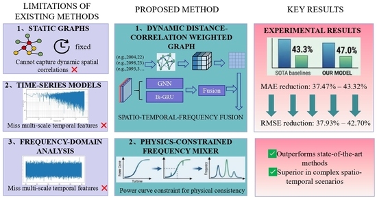
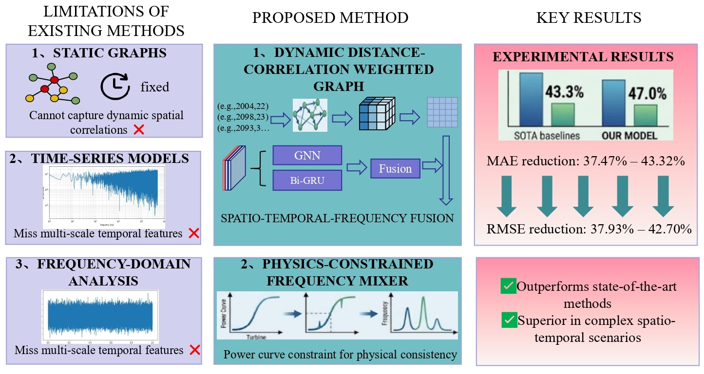
High-precision wind power prediction improves grid stability and reduces curtailment losses. Existing methods face three limitations: static graphs cannot capture dynamic spatial correlations under weather changes, time series models miss multi-scale temporal features, and frequency-domain analyses lack physical constraints. We propose: (1) a dynamic distance correlation weighted graph that adaptively combines geographic and power correlations for weather–terrain coupling; (2) a spatio-temporal-frequency fusion framework integrating graph networks, bidirectional GRUs, and a patchwise sparse time–frequency module; (3) a turbine power curve-constrained frequency mixer for physical consistency. On the SDWPF dataset, our model achieves MAE reductions of 37.47–43.32% and RMSE reductions of 37.93–42.70% versus baselines, outperforming state-of-the-art methods. The approach demonstrates superior performance in complex spatio-temporal scenarios.

1. Introduction

With the accelerating global transition to low-carbon energy systems, wind power has emerged as a pivotal clean and renewable energy source, progressively increasing its share in the power system [1]. Yet, wind power generation exhibits obvious intermittency and volatility due to dynamic coupling of meteorological conditions, geographical distribution, and equipment operational states, posing substantial challenges to grid operations, electricity market participation, and wind farm maintenance [2,3]. Statistics show that high-precision wind power prediction can reduce the wind abandonment rate by 15–20%, yielding annual operational cost savings exceeding millions of dollars for grid operators [4]. Thus, developing high-precision and robust wind power prediction models has become a focus in both academia and industry [5].

Over the past few years, remarkable advancements have been made in wind power forecasting research, covering a wide spectrum of methodologies including physical models, statistical approaches, conventional machine learning techniques, and deep learning-based frameworks. Each category of methods has demonstrated unique merits in addressing partial forecasting demands, yet persistent bottlenecks remain unresolved in practical engineering scenarios. Existing methods are plagued by prominent defects: static graph construction strategies fail to perceive dynamic spatial dependencies driven by variable meteorological conditions and wake effects; traditional time series modeling architectures lack the capability to extract multi-scale temporal and frequency-domain features; and most data-driven models neglect the integration of physical constraints, resulting in insufficient interpretability and unstable prediction performance. These inherent limitations severely restrict the improvement of forecasting accuracy and the industrial application potential of current models.

Targeting the above-mentioned core challenges, this study develops an innovative graph-guided deep learning framework named DBFP-Net (dynamic graph-bidirectional frequency-physics integrated network), which fuses dynamic spatial modeling, bidirectional temporal analysis and constrained time–frequency processing to enhance the precision and robustness of short-to-medium term wind power prediction. The framework breaks through the bottlenecks of traditional methods by optimizing spatial correlation modeling, time–frequency feature extraction and physical constraint integration, providing a feasible solution for efficient and accurate wind power forecasting.

The principal contributions of this work are summarized as follows:

Contribution 1: A novel dynamic weighted graph construction method (DCWGC) is proposed to adaptively model meteorology–terrain coupling and wake effects. By dynamically fusing turbine geographic distance and historical power correlation weights via learnable parameters, it breaks the limitations of static graphs and significantly improves spatial modeling accuracy.

Contribution 2: An innovative time-space-frequency multimodal prediction framework is constructed, integrating DCWGC-based GCN for spatial dependence, BiGRU for temporal feature extraction, and the original PSSTF module for rFFT-based noise separation and frequency feature mining, which markedly boosts forecast accuracy over 10 min to 2 h prediction horizons.

Contribution 3: A physics-constrained frequency-domain noise suppression strategy is designed via the PSSTF module. The novel power curve-constrained frequency mixer ensures aerodynamic compliance while retaining dominant frequency components, unifying physical realism and high-precision prediction.

The rest of the paper is organized as follows: Section 2 systematically reviews the related work in wind power forecasting. Section 3 elaborates the problem formulation of spatio-temporal multi-step wind power prediction and the detailed design of the proposed DBFP-Net model. Section 4 presents the experimental configurations, comparative results and in-depth analysis. Section 5 discusses the critical limitations and future research directions of the proposed method. concludes this paper.

2. Literature Review

In recent years, remarkable progress has been witnessed in the field of wind power prediction, and mainstream research methodologies can be categorized into physical approaches, statistical models, traditional machine learning algorithms and deep learning frameworks [4]. Physical models construct atmospheric dynamic equations relying on numerical weather prediction (NWP) data, but they are plagued by excessively high modeling complexity and prohibitive computational costs [6]. Statistical models, typified by ARIMA and VAR, improve operational efficiency by fitting the inherent relationships in historical data [7], yet their capability to capture nonlinear and multi-scale features embedded in wind power series is severely limited [8]. Traditional machine learning methods including support vector machines (SVMs) and random forest (RFs) are heavily reliant on manual feature engineering, making it difficult to adapt to the dynamic fluctuations of high-dimensional spatio-temporal data [9]. Although the aforementioned methods have improved prediction accuracy to varying degrees, most models are constrained by insufficient ability to characterize the spatio-temporal dynamic coupling relationship, presenting prominent defects especially in modeling the complex spatial correlations of wind turbine clusters. To address the challenges of high volatility, nonlinearity and multi-scale data characteristics, Liu et al. [10] proposed a collaborative multi-resolution ensemble model integrating real-time decomposition and binary kernel density estimation to enhance prediction performance. Nevertheless, statistical models suffer from inherent drawbacks including excessive dependence on historical data, limited generalization ability and slow convergence speed.

Subsequently, various traditional machine learning algorithms have been widely applied to wind power forecasting, such as SVM, Random Forest and BP neural networks [11,12,13]. Yang et al. developed a data-driven finite-state Markov chain model using actual wind farm operation data, which integrates diurnal and seasonal fluctuations of wind power generation and incorporates SVM prediction results to boost performance. Zhang et al. [14] adopted an optimized particle swarm optimization algorithm to refine BP neural network for short-term wind power prediction, effectively elevating prediction accuracy with superior performance in RMSE and MAE compared to the standard PSO-BP method. However, these traditional machine learning approaches invariably involve cumbersome feature engineering, which not only increases computational complexity but also leads to excessively time-consuming prediction procedures.

To overcome the shortcomings of traditional machine learning, deep learning methods have been increasingly introduced into wind power prediction. Zhu et al. [15] proposed a short-term wind power prediction method based on temporal convolutional networks, which excels in capturing temporal dependence but exhibits unsatisfactory performance in handling complex nonlinear features. Shahid et al. [16] developed an LSTM model integrated with genetic algorithm for parameter optimization, which achieves optimal hyperparameter configuration but entails lengthy iterative computation.

Traditional single neural network models are prone to local minima and overfitting; thus, hybrid models have been widely adopted in wind power forecasting. Chen et al. [17] proposed the EnsemLSTM model, which fuses a long short-term memory network, support vector regression, and an extremal optimization algorithm. By employing an LSTM cluster with diverse hidden layers and neuron configurations, EnsemLSTM effectively mines latent information in wind speed time series, yet its performance is highly restricted by complex feature engineering and heavy reliance on feature extraction quality. Zhao et al. [18] put forward a novel nonlinear hybrid model combining singular spectrum analysis and temporal convolutional network, which decomposes raw sequence data and extracts key temporal features via TCN, significantly improving prediction accuracy but consuming massive computational resources.

Meanwhile, graph convolutional networks (GCNs) have provided a novel solution for spatio-temporal prediction of wind turbine clusters owing to their superior capability in modeling non-Euclidean spatial relations and have been extensively employed in such prediction tasks [19,20]. Most existing studies establish inter-turbine connections based on single topological indicators such as geographical distance or linear correlation metrics. For instance, Geng et al. [21] constructed a static graph using geographical distance information and combined it with LSTM to extract temporal dependencies, but such methods fail to capture the dynamic physical and meteorological interactions among turbines. Furthermore, Bentsen et al. [22] extracted spatial dependencies and fused temporal update functions through a GNN architecture. Additionally, Yu et al. [23] proposed a superposition graph neural network (SGNN) that captures spatio-temporal features by constructing and superimposing graphs over sequential time steps. While this superposition mechanism incorporates temporal evolution, the underlying graph at each time step typically relies on fixed spatial relationships (e.g., geographical proximity), which may not adaptively reflect the complex, weather-driven dynamic coupling (e.g., varying wake effects) between turbine power outputs and their spatial distribution in real time. This limitation hinders the full representation of dynamic interactions in operational environments [24].

Despite the advances in spatio-temporal feature capture, existing methods are still limited by single-dimension static correlation modeling, which cannot characterize the dynamic spatial correlations under the coupling of meteorology, terrain and equipment multi-physics fields. This further verifies the necessity and innovation of the proposed DBFP-Net framework for addressing the above research gaps.

The core implementation process of the DBFP-Net for wind power prediction is summarized in Algorithm 1, which covers the entire workflow from input data preprocessing to multi-step wind power prediction, including dynamic graph construction, spatio-temporal-frequency feature extraction, and physics-constrained multimodal fusion.

Algorithm 1 DBFP-Net for wind power prediction with dynamic graph and bidirectional temporal-frequency fusion.

Require: Meteorological-turbine data $\mathit{X}\in {\mathbb{R}}^{T\times N\times D}$ (time steps T, turbine number N, feature dimension D: wind speed, direction, temperature, geographic coordinates, historical power, etc.); Historical power sequence $\mathit{P}\in {\mathbb{R}}^{T\times N}$; Forecast horizon H; Sparsity threshold $\tau$; Dynamic balance coefficient $\alpha$; PSSTF hyperparameters ($P_{\mathrm{chunk}},M_{\mathrm{down}},f_c,K$)

Ensure: Multi-step wind power prediction $\widehat{\mathit{Y}}\in {\mathbb{R}}^{H\times N}$ (MW)

1: Initialization: GCN, Bi-GRU, PSSTF, and fusion layer parameters $\theta =\{{\theta }_{\mathrm{GCN}},{\theta }_{\mathrm{BiGRU}},{\theta }_{\mathrm{PSSTF}},{\theta }_{\mathrm{fusion}}\}$; Min-Max normalization function $\mathrm{Norm}(·)$; Power curve constraint function $\mathrm{PC}(·)$   2: ${\mathit{X}}_{\mathrm{norm}}=\mathrm{Norm}\left(\mathit{X}\right)$ {Normalize all features to [0,1]}   3: ${\mathit{P}}_{\mathrm{norm}}=\mathrm{Norm}\left(\mathit{P}\right)$ {Normalize historical power sequence}   4: for each turbine pair $(v_i,v_j)$ do   5:     $d_{ij}=\mathrm{Euclidean}\mathrm{distance}\mathrm{of}(v_i,v_j)\mathrm{geographic}\mathrm{coordinates}$ {Equation (3)}   6:     $c_{ij}=\left|\mathrm{Cov}(P_i,P_j)\right|/({\sigma }_{P_i}·{\sigma }_{P_j})$ {Power correlation coefficient}   7:     $M_{ij}=\alpha ·\mathrm{Norm}\left(c_{ij}\right)+(1-\alpha )·\mathrm{Norm}(1/d_{ij})$ {Dynamic weight calculation (Equation (2))}   8: end for   9: ${\mathit{A}}_{ij}=M_{ij}\mathrm{if}{M}_{ij}>\tau \mathrm{else}0;{\mathit{A}}_{ii}=0$ {Remove self-connections (Equation (3))} 10: $\mathcal{G}=(\mathit{A},{\mathit{X}}_{\mathrm{norm}})$ {Construct dynamic graph $\mathcal{G}$} 11: ${\mathit{H}}_0={\mathit{X}}_{\mathrm{norm}}.\mathrm{reshape}(T\times N,D)$ {Initial node features} 12: for$l=1 \mathbf{to}$$L_{\mathrm{GCN}}$ do 13:     $\tilde{\mathit{D}}=\mathrm{Degree}(\mathit{A}+\mathit{I})$ {Degree matrix of $\mathit{A}+\mathit{I}$} 14:     ${\mathit{H}}_{l+1}=\sigma ({\tilde{\mathit{D}}}^{-1/2}·(\mathit{A}+\mathit{I})·{\tilde{\mathit{D}}}^{-1/2}·{\mathit{H}}_l·{\mathit{W}}_l)$ {Equation (4)} 15: end for 16: ${\mathit{H}}_{\mathrm{space}}={\mathit{H}}_{L_{\mathrm{GCN}}}.\mathrm{reshape}(T,N,d_s)$ {Spatial features, $d_s$: GCN output dimension} 17: ${\mathit{H}}_{\mathrm{forward}}={\mathrm{GRU}}_{\mathrm{forward}}({\mathit{X}}_{\mathrm{norm}},{\theta }_{{\mathrm{GRU}}_f})$ {Forward GRU (t=1→T)} 18: ${\mathit{H}}_{\mathrm{backward}}={\mathrm{GRU}}_{\mathrm{backward}}({\mathit{X}}_{\mathrm{norm}},{\theta }_{{\mathrm{GRU}}_b})$ {Reverse GRU (t=T→1)} 19: ${\mathit{H}}_{\mathrm{time}}=\mathrm{Concat}({\mathit{H}}_{\mathrm{forward}},{\mathit{H}}_{\mathrm{backward}})$ {Bidirectional temporal features (Equation (9))} 20: ${\mathit{H}}_{\mathrm{time}}=\mathrm{Norm}\left({\mathit{H}}_{\mathrm{time}}\right)$ {Normalize temporal features} 21: ${\mathit{X}}_{\mathrm{reshaped}}={\mathit{X}}_{\mathrm{norm}}.\mathrm{reshape}(T,N\times D)$ 22: ${\mathit{X}}_{\mathrm{chunk}}=\mathrm{Split}({\mathit{X}}_{\mathrm{reshaped}},P_{\mathrm{chunk}})$ {Chunked downsampling (Equation (10))} 23: ${\mathit{X}}_{\mathrm{sample}}=\mathrm{Downsample}({\mathit{X}}_{\mathrm{chunk}},M_{\mathrm{down}})$ {M-fold downsampling} 24: ${\mathit{X}}_{\mathrm{rFFT}}=\mathrm{Trunc}(\mathrm{rFFT}\left({\mathit{X}}_{\mathrm{sample}}\right),f_c)$ {rFFT + dominant frequency truncation} 25: ${\mathit{X}}_{\mathrm{SFM}}=0$ 26: for$k=1 \mathbf{to}$ K do 27:     ${\mathit{X}}_{{\mathrm{rFFT}}_k}=\mathrm{Split}({\mathit{X}}_{\mathrm{rFFT}},K)\left[k\right]$ {Divide into K orthogonal subgroups} 28:     ${\mathit{X}}_{\mathrm{SFM}}+={\mathcal{L}}_k\left({\mathit{X}}_{{\mathrm{rFFT}}_k}\right)$ {Complex linear transformation (Equation (11))} 29: end for 30: ${\mathit{X}}_{\mathrm{SFM}}={\mathit{X}}_{\mathrm{SFM}}+{\mathit{X}}_{\mathrm{rFFT}}$ {Residual connection} 31: ${\widehat{\mathit{X}}}_{\mathrm{rFFT}}=\mathrm{Predictor}({\mathit{X}}_{\mathrm{SFM}},H,{\theta }_{\mathrm{PSSTF}})$ {Future H-step frequency features} 32: ${\widehat{\mathit{X}}}_{\mathrm{rFFT}}=\mathrm{PC}\left({\widehat{\mathit{X}}}_{\mathrm{rFFT}}\right)$ {Apply turbine power curve constraint} 33: ${\widehat{\mathit{X}}}_{\mathrm{time}}=\mathrm{Re}\left(\mathrm{irFFT}\left(\mathrm{ZeroPad}\left({\widehat{\mathit{X}}}_{\mathrm{rFFT}}\right)\right)\right)$ {Inverse rFFT (Equation (12))} 34: ${\mathit{H}}_{\mathrm{freq}}={\widehat{\mathit{X}}}_{\mathrm{time}}.\mathrm{reshape}(H,N,d_f)$ {Frequency features, $d_f$: PSSTF output dimension} 35: ${\mathit{H}}_{\mathrm{space}\_\mathrm{align}}=\mathrm{Align}({\mathit{H}}_{\mathrm{space}},H)$ {Align spatial features to forecast horizon H} 36: ${\mathit{H}}_{\mathrm{time}\_\mathrm{align}}=\mathrm{Align}({\mathit{H}}_{\mathrm{time}},H)$ {Align temporal features to forecast horizon H} 37: $\mathit{C}=\mathrm{Concat}({\mathit{H}}_{\mathrm{space}\_\mathrm{align}},{\mathit{H}}_{\mathrm{time}\_\mathrm{align}},{\mathit{H}}_{\mathrm{freq}})$ {Feature concatenation (Equation (13))} 38: $\widehat{\mathit{Y}}={\mathit{W}}_2·\mathrm{GeLU}({\mathit{W}}_1·\mathit{C}+b_1)+b_2$ {Fusion prediction (Equation (14))} 39: $\widehat{\mathit{Y}}=\mathrm{Denorm}\left(\widehat{\mathit{Y}}\right)$ {Denormalize to original MW scale} 40: return $\widehat{\mathit{Y}}$

3. Methodology

3.1. Problem Formulation

The power output of wind turbines is jointly determined by a variety of complex and interrelated factors [25], including meteorological conditions (e.g., wind speed, wind direction, barometric pressure, and temperature), geographic topological location, and temporal variation characteristics [26]. To address the challenges of wind power intermittency and volatility for grid operation, this study focuses on developing a high-precision wind power prediction model whose core objective is to minimize the deviation between the predicted power value and the actual output power. The optimization objective of the model is mathematically formulated as:

$$\underset{\theta }{min}\sum _{t=1}^T{(f(X_t;\theta )-Y_t)}^2$$

(1)

where $f(·;\theta )$ denotes the data-driven predictive model function with trainable parameter set $\theta$, $X_t$ is the input feature set at historical moment t (consisting of meteorological time series data and geographic coordinates of all turbines in the wind farm), and $Y_t$ represents the true active power output of the wind turbine cluster at moment t.

On this basis, the study targets the **multi-step wind power prediction task** in practical scenarios: the model takes a continuous historical data window with length L (i.e., $X_{t-L+1},X_{t-L+2},\dots ,X_t$) as the input and learns the spatio-temporal correlation of the data to predict the power output sequence of the next H time steps, which is expressed as ${\widehat{Y}}_{t+1},\dots ,{\widehat{Y}}_{t+H}=f(X_{t-L+1},\dots ,X_t;\theta )$.

Notably, the key difficulty of this multi-step prediction task lies in the **dynamic coupling interaction of spatio-temporal elements** in the wind farm: on the one hand, the model needs to effectively extract the inherent periodic and trend features from the non-stationary wind power time series; on the other hand, it is necessary to accurately model the complex spatial dependencies between individual turbines (e.g., wake effect and power coupling effect) based on their geographic coordinates and actual operation data. The above two aspects of feature learning need to be realized simultaneously to ensure the accuracy of multi-step wind power prediction.

3.2. Overview of the Modeling Framework

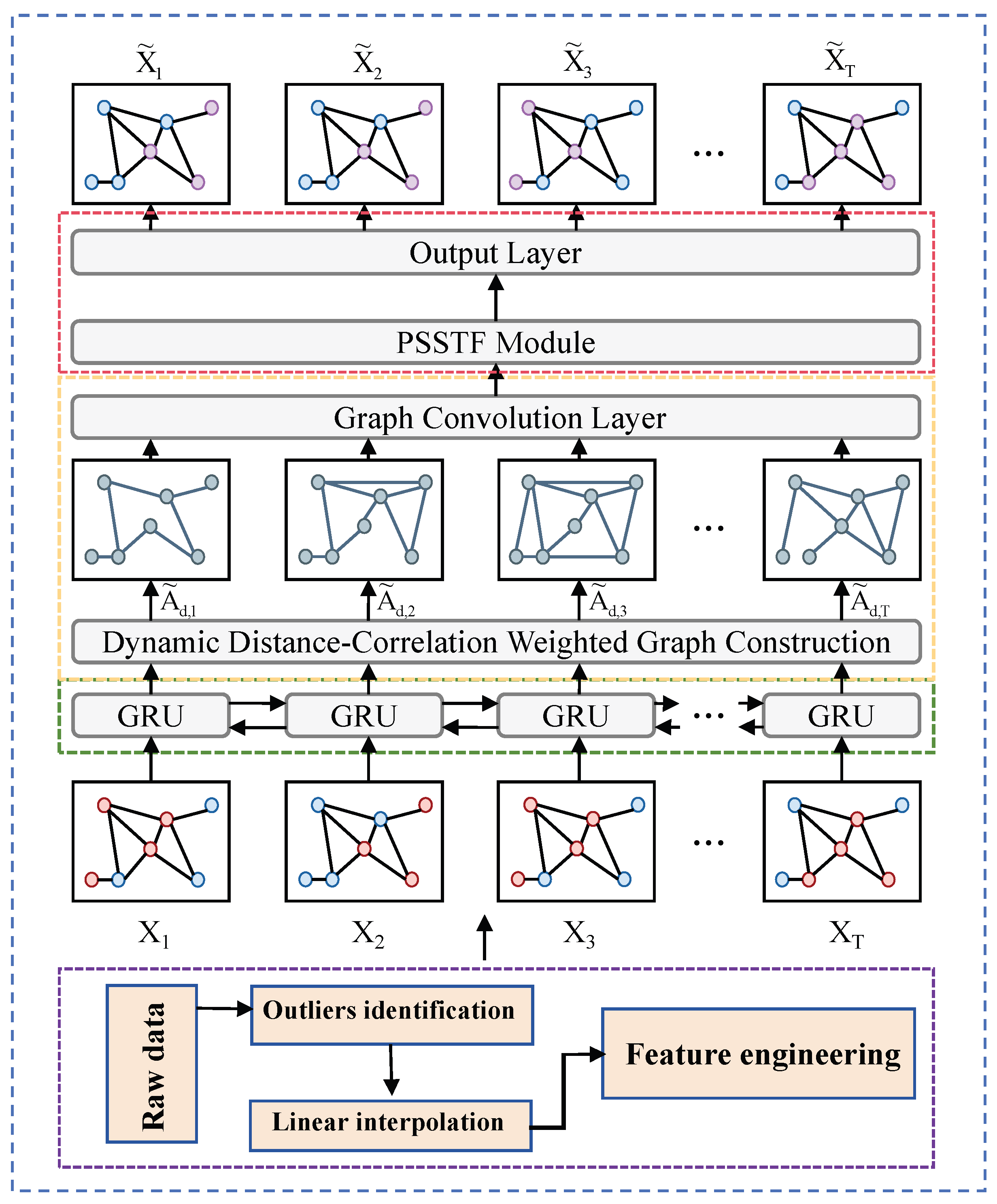
Aiming at the complexity of meteorological-terrain-equipment multifactor coupling and spatio-temporal-frequency multiscale feature intertwining in wind power prediction, this study proposes a novel dynamic graph and bidirectional temporal-frequency fusion network (DBFP-Net), whose multimodal fusion framework is shown in Figure 1.

3.3. Dynamic Spatial Graph Feature Modeling

The spatial correlation characteristics between wind turbines play a key role in power generation prediction, which not only reflects the spatial propagation law of meteorological elements such as wind speed and wind direction [27], but also directly affects the power coupling effect between units. Traditional methods mostly use static topological modeling, which is difficult to adapt to the dynamic changes of turbine interactions under complex meteorological conditions. For this reason, this paper proposes a dynamic distance correlation weighted graph construction (DCWGC) method, which builds an adaptive graph structure by coupling geographic distance and power correlation, and realizes deep spatial feature extraction by combining graph convolutional networks.

3.3.1. Dynamic Distance Correlation Weighted Graph Construction

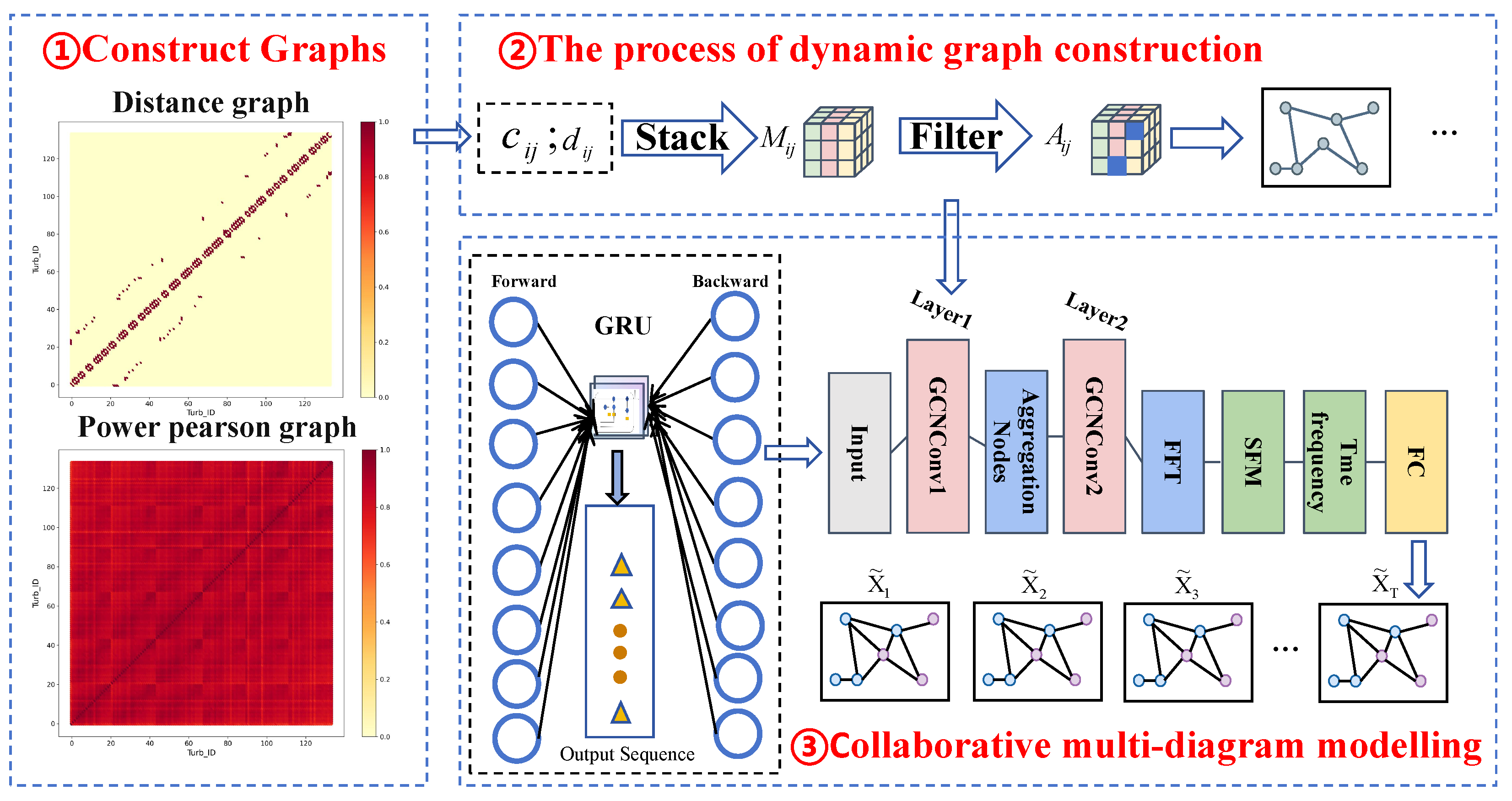
The core of DCWGC lies in the dynamic optimization of connection weights between nodes relying on learnable parameters. The construction process of the dynamic graph is detailed in Figure 2, which contains the following two key steps:

Define the association weights of any two turbines $v_i$ and $v_j$ as:

$$M_{ij}=\alpha ·\mathrm{Norm}\left(c_{ij}\right)+(1-\alpha )·\mathrm{Norm}(1/d_{ij})$$

(2)

where $c_{ij}$ denotes the power dynamic correlation between turbine $v_i$ and $v_j$, calculated from the absolute correlation coefficients of their power time series $P_i$ and $P_j$: $c_{ij}={\displaystyle \frac{\left|\mathrm{Cov}\right(P_i,P_j\left)\right|}{{\sigma }_{P_i}·{\sigma }_{P_j}}}$; $d_{ij}$ is the geographic Euclidean distance between turbines $v_i$ and $v_j$, calculated from their geographic coordinates $(x_i,y_i)$ and $(x_j,y_j)$: $d_{ij}=\sqrt{{(x_i-x_j)}^2+{(y_i-y_j)}^2}$; $\alpha \in [0,1]$ is the learnable dynamic balance coefficient that regulates the weight share of power correlation and geographic distance in graph construction.

Implementation Details of $\alpha$: 1. Initialization: $\alpha$ is initialized to 0.5 (assigning equal weight to geographic distance and power correlation) using a uniform distribution $\mathcal{U}(0.4,0.6)$, which can effectively avoid extreme initial values and stabilize the early training process of the model; 2. Loss Function for Optimization: $\alpha$ is jointly optimized with all other model parameters via the mean squared error (MSE) loss defined in Equation (1), and the total loss function is updated as: $\mathcal{L}={\sum }_{t=1}^T{(f(X_t;\theta ,\alpha )-Y_t)}^2$, where $\theta$ includes all neural network parameters of GCN, Bi-GRU and fusion layers, and $\alpha$ is treated as a trainable scalar parameter; 3. Training Behavior: During the backpropagation process, $\alpha$ is updated synchronously with other parameters using the Adam optimizer (with a fixed learning rate of $1\times {10}^{-4}$), and gradient clipping (max norm of 1.0) is adopted to prevent unstable parameter updates caused by excessive gradient. Empirically, $\alpha$ stably converges to $0.65\pm 0.08$ in the training process, which indicates that power correlation contributes more than geographic distance in the dynamic graph construction for wind power prediction.

$\mathrm{Norm}(·)$ denotes the min-max normalization function that maps the heterogeneous features $c_{ij}$ and $1/d_{ij}$ to the unified interval [0,1], and its specific definition is $\mathrm{Norm}\left(x\right)={\displaystyle \frac{x-min\left(x\right)}{max\left(x\right)-min\left(x\right)}}$.

To reduce the noise interference of weak correlation edges and improve the computational efficiency of graph convolution, the obtained weight matrix M is further processed by threshold filtering:

$$A_{ij}=\left\{\begin{array}{cc}{M}_{ij},\hfill & M_{ij}>\tau \hfill \\ 0,\hfill & M_{ij}\le \tau \hfill \end{array}\right.$$

(3)

where $\tau$ is a preset sparsity threshold, which is determined to be 0.1 via grid search on the validation set (search range: 0.05∼0.25) and fixed in all experiments. During filtering, the self-connecting edges are removed (i.e., $A_{ii}=0$), which ultimately generates a sparse adjacency matrix $A\in {\mathbb{R}}^{N\times N}$, where nodes characterize individual wind turbines in the farm, and edge weights characterize the spatial-dynamic coupling strength between different turbines.

3.3.2. Graph Convolution Feature Extraction

Based on the adaptive graph structure $G=(A,X)$ generated by DCWGC, a multilayer graph convolutional network (GCN) is used to aggregate the neighborhood feature information of each turbine node, and its single-layer propagation rule is defined as

$$H^{(l+1)}=\sigma \left({\tilde{D}}^{-{\displaystyle \frac{1}{2}}}\tilde{A}{\tilde{D}}^{-{\displaystyle \frac{1}{2}}}{H}^{\left(l\right)}{W}^{\left(l\right)}\right)$$

(4)

where $\tilde{A}=A+I$ is the adjacency matrix with self-connections added to retain the original feature information of each node; $\tilde{D}$ is the degree matrix of $\tilde{A}$ with ${\tilde{D}}_{ii}={\sum }_j{\tilde{A}}_{ij}$; $H^{\left(l\right)}$ is the node feature matrix of the l-th GCN layer; $W^{\left(l\right)}$ is the trainable weight matrix of the l-th layer; and $\sigma (·)$ is the ReLU nonlinear activation function selected for stable gradient propagation and effective feature nonlinear mapping.

By stacking multiple layers of GCNs (2 layers are used in experiments), the model is able to capture the multi-order spatial dependencies of the wind turbine cluster layer by layer from local to global. The final output of the GCN is the high-dimensional spatial feature matrix $H_{\mathrm{space}}\in {\mathbb{R}}^{N\times d}$ (with feature dimension $d=64$), which provides the spatial feature basis for the subsequent spatio-temporal-frequency multimodal feature fusion.

3.4. Bidirectional Time Series Meteorological Feature Extraction

Wind power data exhibit significant non-stationarity and randomness due to the influence of meteorological periodicity, diurnal cycles, and seasonal factors [27]. To effectively model the temporal correlation and hysteresis characteristics of wind power time series, we employ a bidirectional gated recurrent unit (Bi-GRU) architecture that processes the sequence data in both forward and reverse temporal directions [28]. This bidirectional design can not only capture the regular meteorological evolution patterns but also effectively identify the hysteresis effects caused by turbine wake disturbances [29].

• Core Mechanisms: 1. Forward GRU ($t=1\to T$): Processes the historical meteorological and power time series in the forward time direction to capture the inherent daily/seasonal periodic features and trend changes of the data; 2. Reverse GRU ($t=T\to 1$): Analyzes the same time series in the reverse time direction to detect the delayed response characteristics of wind turbine power output to turbulent disturbances and sudden meteorological changes.
• Gate Operations: The forward and reverse GRUs share the same gate operation mechanism, and the core calculation process of a single GRU unit is as follows:

  $$\begin{array}{cccc}\hfill & \mathrm{Update}\mathrm{Gate}:\hfill & \hfill z_t& =\sigma (W_z·[h_{t-1},x_t]+b_z)\hfill \end{array}$$

  (5)

  $$\begin{array}{cccc}\hfill & \mathrm{Reset}\mathrm{Gate}:\hfill & \hfill r_t& =\sigma (W_r·[h_{t-1},x_t]+b_r)\hfill \end{array}$$

  (6)

  $$\begin{array}{cccc}\hfill & \mathrm{Candidate}\mathrm{State}:\hfill & \hfill {\tilde{h}}_t& =tanh(W_h·[r_t\odot h_{t-1},x_t]+b_h)\hfill \end{array}$$

  (7)

  $$\begin{array}{cccc}\hfill & \mathrm{State}\mathrm{Update}:\hfill & \hfill h_t& =(1-z_t)\odot h_{t-1}+z_t\odot {\tilde{h}}_t\hfill \end{array}$$

  (8)

  where $x_t$ contains the normalized meteorological and power features at moment t, $h_{t-1}$ is the hidden state of the GRU at the previous moment and encodes the historical power change trends, ⊙ denotes the element-wise multiplication operation, and $W_z,W_r,W_h$ and $b_z,b_r,b_h$ are the trainable weight matrices and bias vectors of the GRU gates, respectively.
• Feature Fusion: The hidden state sequences output by the forward and reverse GRUs are concatenated along the feature dimension to form the complete bidirectional temporal features, which is expressed as

  $$H_{\mathrm{time}}=[H^{\to }\Vert H^{\leftarrow }]\in {\mathbb{R}}^{T\times 2h}$$

  (9)

  where $h=64$ is the hidden dimension of a single forward/reverse GRU and the final temporal feature dimension is set to 128 to ensure that the temporal feature dimension matches the spatial feature dimension for subsequent multimodal fusion.

This joint bidirectional temporal representation can fully preserve the complete meteorological evolution patterns and power change characteristics of the time series while effectively suppressing the random turbulent noise in the data. Subsequent ablation experiments in Section 4.5.1 further confirm the superiority of the bidirectional structure over the traditional unidirectional RNN/GRU in wind power time series modeling.

3.5. Chunked Sparse Time–Frequency Feature Fusion and Multimodal Feature Co-Prediction

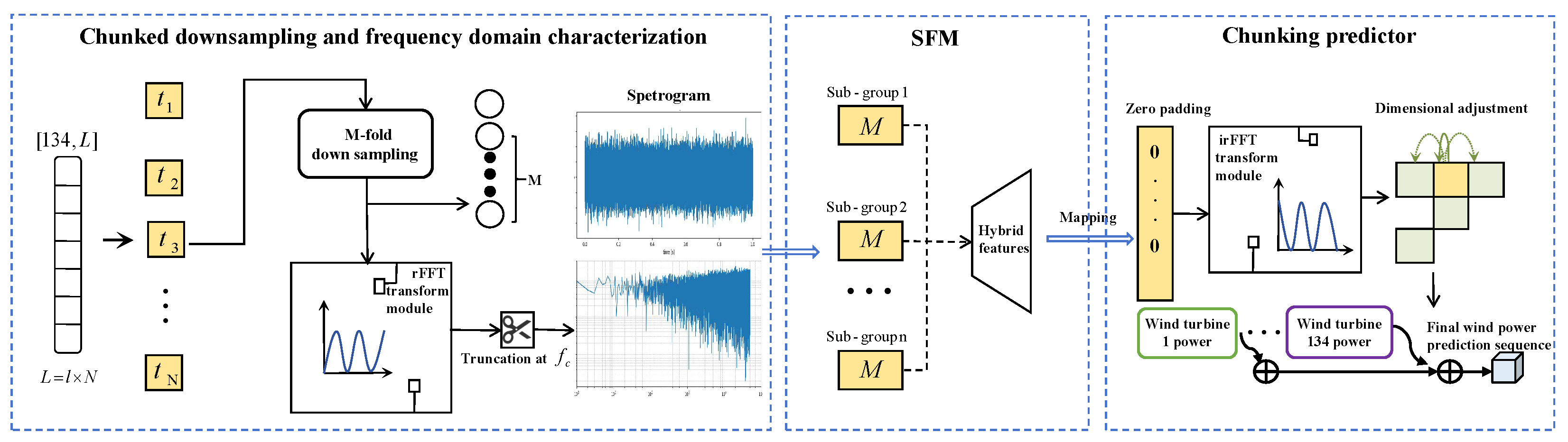
The wind power time series exhibits strong non-stationary behavior with superimposed low-frequency trend features, mid-frequency periodic fluctuation features, and high-frequency transient perturbation features. To fully model these multi-scale frequency characteristics and separate the valid signal from noise, we propose a patchwise sparse time–frequency (PSSTF) module, whose detailed architecture is shown in Figure 3, and the core workflow is divided into the following three steps.

3.5.1. Chunked Downsampling and Frequency Domain Characterization

The original one-dimensional time series input $\mathit{x}\in {\mathbb{R}}^L$ is first partitioned into P non-overlapping local chunks (with each chunk length $L_P=L/P$) to capture the local frequency fluctuations of different time periods. Each local chunk is then downsampled by M-fold ($M=\lfloor f_s/\left(2f_{\max }\right)\rfloor$, where $f_s=1/6$ Hz is the sampling frequency for 10 min interval data) to produce the downsampled feature tensor ${\mathit{x}}_{\mathrm{sample}}\in {\mathbb{R}}^{P\times {\displaystyle \frac{L}{PM}}\times M}$, which can preserve the key wind speed-power coupling characteristics while significantly reducing the computational complexity of subsequent frequency domain analysis. The downsampled data is converted to the frequency domain via real-valued fast Fourier transform (rFFT), and the high-frequency components beyond the dominant frequency threshold $f_c$ are truncated to filter out the high-frequency turbulent noise:

$$x_{\mathrm{rFFT}}=\mathrm{Trunc}\left(\mathrm{rFFT}\right(x_{\mathrm{sample}}\left)\right)\in {\mathbb{C}}^{P\times f_c\times M}$$

(10)

where $\mathrm{Trunc}(·)$ is the frequency truncation function that only retains the dominant frequency components corresponding to the wind speed periodicity (0.01–0.1 Hz), and $f_c$ is set to 10 in all experiments to balance the frequency feature integrity and noise suppression effect.

3.5.2. Sparse Frequency Mixing Mechanism

To effectively model the harmonic components of the dominant frequency and suppress the spectral leakage phenomenon in frequency domain conversion, the retained $f_c$ frequency components are divided into K orthogonal subgroups (with $f_c/K$ components in each subgroup, $K=4$ in experiments). Each subgroup is processed by an independent complex linear transformation $L_k$ with block-diagonal weight matrices, which can reduce the number of model parameters by a factor of $1-1/K$. The sparse frequency mixing output is obtained by concatenating the transformed features of all subgroups and adding the original frequency features via residual connection:

$$X_{\mathrm{SFM}}={\mathrm{Concat}}_{k=1}^K{L}_k\left(X_{\mathrm{rFFT}}^{\left(k\right)}\right)+X_{\mathrm{rFFT}}$$

(11)

This residual design can retain the original dominant frequency trend features while enhancing the modeling ability of harmonic components, and effectively suppress the high-frequency tower shadow interference (high-frequency noise > 0.1 Hz) in the wind farm.

3.5.3. Cross-Segment Trend Forecasting and Time-Domain Reconstruction

A parameter-sharing frequency domain predictor (with a total of ${\displaystyle \frac{P^{2}H}{L}}$ trainable parameters) is used to map the sparse frequency mixing features $X_{\mathrm{SFM}}\in {\mathbb{C}}^{P\times f_c\times M}$ to the future H-step frequency domain components $\widehat{X}\in {\mathbb{C}}^{{\displaystyle \frac{PH}{L}}\times f_c\times M}$, and the physical power curve constraints are incorporated during prediction (i.e., clipping the predicted frequency domain power values to the valid range of [0, rated power] of the turbine to ensure physical consistency). The predicted future frequency domain features are then converted back to the time domain to obtain the time-domain power prediction results via inverse rFFT, and the specific reconstruction process is

$${\widehat{x}}_{\mathrm{irFFT}}=\mathrm{Re}\left(\mathrm{irFFT}\left(\mathrm{ZeroPad}\left(\widehat{X}\right)\right)\right)\in {\mathbb{R}}^H$$

(12)

where $\mathrm{ZeroPad}(·)$ is the zero-padding operation that pads the predicted frequency domain components to match the original time-domain sequence length, and $\mathrm{Re}(·)$ takes the real part of the complex inverse rFFT result to ensure the physical interpretability of the time-domain prediction results (the imaginary part is introduced by numerical calculation and has no actual physical meaning).

The output dimensions of the frequency domain features can adapt dynamically according to the forecast horizon H, and the final frequency domain features ${\widehat{x}}_{\mathrm{irFFT}}$ are resized to the same dimension as the spatial and temporal features, with spatial graph features added to generate the final frequency feature matrix $\widehat{x}\in {\mathbb{R}}^H$.

3.6. Collaborative Prediction of Multimodal Features

To fully exploit the complementary information of spatial, temporal and frequency features, a three-level multimodal feature fusion strategy is adopted to integrate the spatial features ($S=H_{\mathrm{space}}$), temporal features ($T=H_{\mathrm{time}}$), and frequency features ($F={\widehat{x}}_{\mathrm{irFFT}}$) extracted by the above three modules. The feature concatenation operation is performed along the feature dimension to form the comprehensive multimodal feature matrix:

$$C=\mathrm{Concat}(S,T,F)\in {\mathbb{R}}^{B\times N\times (D_s+D_t+D_f)}$$

(13)

where B is the training batch size, $N=134$ is the total number of turbines in the wind farm, and $D_s=D_t=D_f=64$ are the unified feature dimensions of the three modal features (realized by dimension adjustment).

The final wind power multi-step prediction results are generated via a lightweight two-layer fully connected network with nonlinear activation, which is defined as

$$\widehat{y}=W_2·\mathrm{GeLU}(W_1·C+b_1)+b_2\in {\mathbb{R}}^{B\times N\times H}$$

(14)

where $W_1\in {\mathbb{R}}^{(D_s+D_t+D_f)\times d}$ (with hidden dimension $d=64$) and $W_2\in {\mathbb{R}}^{d\times H}$ are the trainable weight matrices of the two fully connected layers, $b_1$ and $b_2$ are the corresponding bias vectors, and the GeLU activation function is used for smooth gradient flow and effective nonlinear feature mapping to avoid the gradient disappearance problem in deep fully connected networks.

4. Experiment

4.1. Data Description

To verify the performance of the proposed DBFP-Net model in high-precision wind power prediction under meteorology-terrain coupling conditions, this study conducts all experiments on the public Spatial Dynamic Wind Power Forecasting (SDWPF) dataset [30]. The dataset is collected from a large-scale wind farm in China with 134 operating wind turbines, covering the SCADA-synchronized monitoring data from January to June 2022 (245 continuous operation days), with a total of 4,727,520 data records at a 10-min sampling interval. Each record contains 13 monitoring variables, and the key variables used in this study include: Wspd (wind speed), Wdir (wind direction), Etmp (environment temperature), Itmp (turbine inner temperature), Ndir (nacelle direction), Pab1-3 (three blade pitch angles), Prtv (reactive power), and the target variable Patv (active power output, in MW).

4.2. Experimental Settings

To strike a balance between the model prediction performance and computational cost, all hyperparameters of the DBFP-Net model are optimized via a grid search strategy on the validation set, and the optimal hyperparameter configuration is determined as: learning rate of $1\times {10}^{-4}$, training batch size of 32, and total training epochs of 100. All model predictions are measured in megawatts (MW), and all subsequent evaluation metrics (MAE, RMSE, $R^2$) are also reported in this unit to ensure the consistency of the experimental results. The detailed architecture and trainable parameter count of each component of the DBFP-Net model are listed in

Table 1. Model architecture and detailed parameters.

Model Component/Hyperparameter	Setting/Output Shape	Trainable Param. Count
Sparse Threshold ($\tau$)	0.1 (fixed)	-
Dynamic Balance Coefficient ($\alpha$)	Learnable (initialized to 0.5)	-
PSSTF Chunk Number (P)	8	-
PSSTF Downsampling Factor (M)	2	-
PSSTF Dominant Frequency ($f_c$)	10	-
PSSTF Orthogonal Subgroups (K)	4	-
Learning Rate	$1\times {10}^{-4}$	-
Batch Size	32	-
Dropout Rate	0.2	-
Input Layer	(bs, 134, 72, 14)	-
GCNConv (Layer 1)	(bs × 134 × 72, 64)	$1464+64=960$
GCNConv (Layer 2)	(bs × 134 × 72, 64)	$6464+64=4160$
Batch Normalization (L1)	(bs × 134 × 72, 64)	128
Batch Normalization (L2)	(bs × 134 × 72, 64)	128
PSSTF Module	(bs, 1, 134, 64)	-
Fully Connected (L1)	(bs × 134 × 1, 64)	$6464+64=4160$
Dropout (0.2)	(bs × 134 × 1, 64)	0
Fully Connected (L2)	(bs × 134 × 1, 1)	$641+1=65$
Total Trainable Parameters	-	10,537

. In addition, the computational complexity and inference efficiency of DBFP-Net are analyzed for practical deployment. The time complexity of the proposed model can be expressed as $O(T·N^2·d+T·N·F·d)$, where T denotes the input sequence length, N is the number of wind turbines, F represents the frequency-domain feature dimension, and d is the hidden dimension. The total floating-point operations (FLOPs) of DBFP-Net are about $2.92\times {10}^9$, and the total trainable parameters are 10537 as shown in Table 1. Due to the introduction of dynamic graph construction and time–frequency fusion modules, the training duration is prolonged by approximately 25% compared with lightweight baseline models, which is quantitatively verified in the subsequent computational cost comparison. The code for our model is available at https://github.com/lulu3939/lulucode (accessed on 3 March 2026).

4.3. Sensitivity Analysis

To verify the robustness of the proposed DBFP-Net to the sparse threshold $\tau$ in Equation (3), we conduct sensitivity analysis by varying $\tau$ within a reasonable range ($0.05,0.10,0.15,0.20,0.25$) while keeping other hyperparameters fixed. As shown in

Table 2. Performance of DBFP-Net under different sparse threshold $\tau$.

$\mathit{\tau }$	10 min			30 min			1 h			2 h
	MAE	RMSE	${\mathit{R}}^{\mathbf{2}}$	MAE	RMSE	${\mathit{R}}^{\mathbf{2}}$	MAE	>RMSE	${\mathit{R}}^{\mathbf{2}}$	MAE	RMSE	${\mathit{R}}^{\mathbf{2}}$
0.05	3.1872	3.8215	0.9768	4.2915	5.0832	0.9382	5.0147	5.8923	0.9345	6.5732	7.3218	0.8726
0.10	3.0236	3.6473	0.9795	4.0736	4.8691	0.9418	4.8271	5.6736	0.9388	6.3047	7.0677	0.8807
0.15	3.2451	3.8967	0.9756	4.3562	5.1548	0.9365	5.1023	5.9874	0.9321	6.6895	7.4532	0.8689
0.20	3.5128	4.1739	0.9712	4.6893	5.4726	0.9301	5.4386	6.3215	0.9257	7.0124	7.7896	0.8593
0.25	3.8764	4.5328	0.9658	5.0217	5.8143	0.9234	5.8642	6.7589	0.9184	7.4568	8.2145	0.8472

, the sparse threshold $\tau$ has a significant impact on the model performance: 1. When $\tau =0.10$, the model achieves the optimal performance across all prediction horizons, with the lowest MAE (3.0236 MW for 10 min, 6.3047 MW for 2 h) and RMSE, and the highest $R^2$ (0.9795 for 10 min, 0.8807 for 2 h). This confirms that $\tau =0.10$ is the optimal value for balancing the sparsity of the adjacency matrix and the integrity of spatial correlation information. 2. When $\tau <0.10$ (e.g., $\tau =0.05$), the adjacency matrix retains too many weak correlation edges, leading to redundant noise in spatial feature extraction and slight performance degradation. 3. When $\tau >0.10$ (e.g., $\tau =0.20,0.25$), the adjacency matrix becomes overly sparse, and key spatial correlation edges between turbines are filtered out, resulting in insufficient capture of wake effects and power coupling, which significantly reduces the prediction accuracy. 4. The model maintains relatively stable performance when $\tau$ is in the range of 0.05∼0.15 (MAE variation < 0.2 MW for 10 min prediction), indicating good robustness to small fluctuations of $\tau$. However, when $\tau$ exceeds 0.20, the performance degrades rapidly, suggesting that excessive sparsity should be avoided in practical applications.

The above sensitivity analysis demonstrates that the selected sparse threshold $\tau =0.10$ is reasonable and optimal, and provides a reference range (0.08∼0.12) for $\tau$ in similar wind power prediction scenarios.

4.4. Comparative Experiments

We compare with baseline and state-of-the-art spatio-temporal prediction methods on the Baidu SDWPF dataset. These models include CNNLSTM [31] for mining spatio-temporal features, DSformer [32] which combines down-sampling and up-sampling for high-dimensional long sequences, DPFMformer [33] that performs frequency-domain modeling via dual-path Mamba-Transformer and integrates meteorological correlation-based error correction, and WPfSRnL [34] integrating random forest feature selection and neural network clustering with BiGRU for prediction. We analyze 10 min (1-step), 30 min (3-step), 1 h (6-step), and 2 h (12-step) multistep forecasts, evaluated by MAE, RMSE, and $R^2$.

Table 3. WPF results generated by existing spatio-temporal models for different forecasting time horizons.

Model	10 min			30 min			1 h			2 h
	MAE	RMSE	${\mathit{R}}^{\mathbf{2}}$	MAE	RMSE	${\mathit{R}}^{\mathbf{2}}$	MAE	RMSE	${\mathit{R}}^{\mathbf{2}}$	MAE	RMSE	${\mathit{R}}^{\mathbf{2}}$
CNNLSTM [31]	4.8802	6.3652	0.96785	7.1876	7.8448	0.92735	7.9954	9.3320	0.86335	10.0826	12.1879	0.84887
DSformer [32]	3.2194	4.2745	0.96709	4.3529	5.1206	0.93276	5.3570	7.2955	0.93114	9.4026	11.2722	0.87256
WPsRmL [34]	3.4235	4.8846	0.96657	4.7970	5.5267	0.93054	6.5286	6.3808	0.89457	7.4415	8.2048	0.85453
DPFMformer [33]	3.1856	4.1923	0.96987	4.2681	4.9835	0.93562	5.1429	6.1058	0.93407	7.1248	8.3369	0.87814
Proposed	3.0236	3.6473	0.97952	4.0736	4.8691	0.94178	4.8271	5.6736	0.93876	6.3047	7.0677	0.88065

shows results for these time ranges.

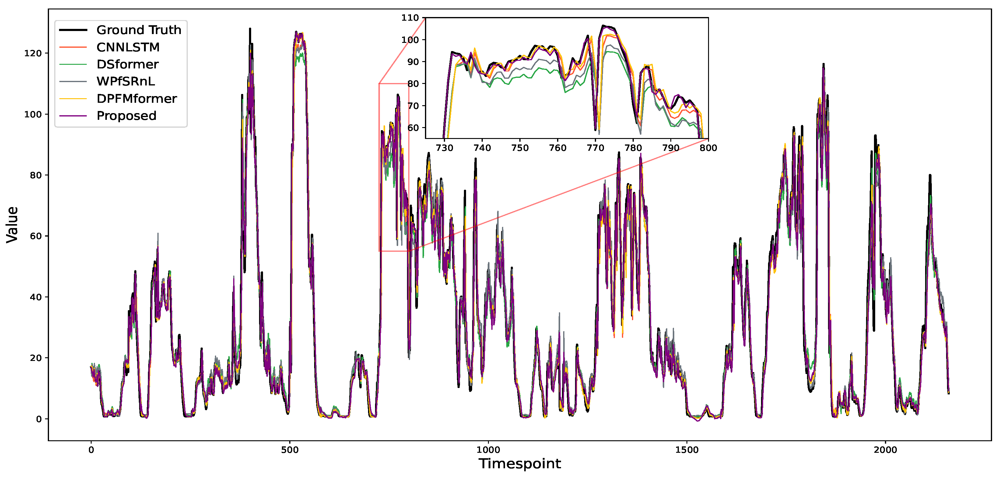
Figure 4 shows temporal performance, with one-step forecasts comparing DBFP-Net and benchmarks. Combined with Figure 5 scatter plots, our DBFP-Net outperforms baselines in one-step prediction. Table 3 confirms DBFP-Net outperforms all baselines across dimensions, showing excellent prediction ability and adaptability. Compared with CNNLSTM [31], it reduces MAE by 38.04%, 43.32%, 39.35%, 37.47% and RMSE by 42.70%, 37.93%, 39.20%, 42.00% for the four multi-step tasks, respectively.

4.5. Ablation Experiments

4.5.1. Ablation Study of PSSTF and Spatio-Temporal-Frequency Multimodal Fusion Modules

Table 4. WPF results using different models in the sequence learning module.

Model	10 min			30 min			1 h			2 h
	MAE	RMSE	${\mathit{R}}^{\mathbf{2}}$	MAE	RMSE	${\mathit{R}}^{\mathbf{2}}$	MAE	RMSE	${\mathit{R}}^{\mathbf{2}}$	MAE	RMSE	${\mathit{R}}^{\mathbf{2}}$
MLP	5.2347	6.8989	0.8234	5.8921	7.5643	0.8054	6.5432	8.2394	0.7823	7.2156	8.9864	0.7531
Transformer	4.8981	6.5475	0.8423	5.4351	7.1221	0.8243	6.0108	7.7895	0.8374	6.7878	8.5401	0.7723
Bi-LSTM	4.5653	6.1279	0.8526	5.1238	6.7877	0.8351	5.7829	7.4541	0.8126	6.4547	8.120	0.7852
TCN	4.7853	6.3426	0.8492	5.6449	6.9861	0.8324	5.9835	7.6543	0.8056	6.6537	8.3406	0.7883
GRU	4.6527	6.2339	0.8438	5.2346	6.8729	0.8432	5.8720	7.5440	0.8308	6.5241	8.2345	0.7832
Bi-GRU	4.3850	6.1010	0.8575	5.1129	6.7501	0.8474	5.6861	7.3627	0.8385	6.4524	8.1280	0.7968
DCWGC-MLP	6.2758	7.1308	0.8841	6.7328	7.1581	0.8485	8.2880	8.9580	0.8154	8.6013	9.7177	0.7052
DCWGC-Trans	4.0221	4.3256	0.9671	5.6254	6.0891	0.9037	6.3912	7.1673	0.8555	8.7571	9.8757	0.7216
DCWGC-LSTM	4.9708	5.2143	0.9296	5.5194	5.9512	0.9166	6.3208	7.0104	0.8539	8.2640	9.3392	0.7259
DCWGC-TCN	5.0808	5.4718	0.9666	4.9855	5.4864	0.9086	6.3567	7.0771	0.8004	10.272	11.210	0.6338
DCWGC-BiGRU	4.4814	4.5706	0.9431	5.3239	5.4789	0.9273	5.5461	6.0838	0.8208	8.4823	9.5169	0.7685
Proposed	3.0236	3.6473	0.9795	4.0736	4.8691	0.94178	4.8271	5.6736	0.9388	6.3047	7.0677	0.8807

shows that the DBFP-Net model exhibits strong capability in learning sequence information from spatio-temporal fusion features, with significant improvements over baseline models like MLP, Transformer, Bi-LSTM, TCN, and GRU. DBFP-Net outperforms other models due to its dynamic weighted graph construction based on turbine distance and power correlation (addressing limitations of traditional static topology methods), bidirectional GRUs that comprehensively model time dependence (overcoming gradient decay in unidirectional RNNs for long time-domain sequences and enhancing periodic weather pattern modeling, unlike unidirectional models such as DCWGC-LSTM/GRU or DCWGC-TCN which struggle with global dependence of non-smooth wind data), and an improved PSSTF module that performs time–frequency analysis and deep fusion with multimodal features. This module maps power sequence segments to the frequency domain, uses frequency truncation and sparse mixing to separate meteorological trends from high-frequency interference (e.g., tower shadow effect), and extracts inter-segment frequency-domain correlations via a lightweight sparse mixer, reducing high-frequency noise by 20.38% through time–frequency filtering and increasing long sequence processing speed by 15.42% with chunked rFFT to balance accuracy and efficiency—unlike DCWGC-MLP and Transformer, which lack such frequency-domain analysis. Ablation experiments confirm DBFP-Net’s advantage in sequence learning, with MAE improvements of 51.82%, 39.50%, 41.76%, 26.70% and RMSE improvements of 48.85%, 32.09%, 37.78%, 27.27% over DCWGC-MLP for 10 min, 30 min, 1 h, and 2 h predictions, respectively.

4.5.2. Ablation Study Analysis of Graph Construction Methods

To evaluate the effectiveness of dynamic graph construction using turbine distance and power correlation in enhancing wind power prediction, we compare several graph construction methods (

Table 5. Different graph construction methods in the proposed framework.

Graph Construction	10 min			30 min			1 h			2 h
	MAE	RMSE	${\mathit{R}}^{\mathbf{2}}$	MAE	RMSE	${\mathit{R}}^{\mathbf{2}}$	MAE	RMSE	${\mathit{R}}^{\mathbf{2}}$	MAE	RMSE	${\mathit{R}}^{\mathbf{2}}$
Distance graph	3.7359	4.3685	0.9216	4.2841	5.2189	0.9163	5.5756	7.0250	0.9088	7.9777	8.4173	0.8773
Pearson graph	3.5637	4.7349	0.9348	4.6435	5.6317	0.9017	5.2952	6.4362	0.8924	7.3223	7.5392	0.8741
DCWGC (Proposed)	3.0236	3.6473	0.9795	4.0736	4.8691	0.94178	4.8271	5.6736	0.9388	6.3047	7.0677	0.8807

). The baseline distance graph, relying solely on physical turbine distances, and the Pearson graph, based on linear correlations of power time series, struggle to capture complex nonlinear relationships. In contrast, the proposed DBFP-Net integrates both distance and power correlation while dynamically adapting to complex patterns, effectively modeling both linear and nonlinear dependencies. Our DCWGC mechanism dynamically fuses geographic distance and power correlation via learnable weights, constructing an adaptive topology that reflects wake effects and turbulence. Ablation experiments show DCWGC reduces MAE by 15.6–22.3% and RMSE by 6.25–22.97% compared to static methods (distance and Pearson graphs), confirming its superiority in modeling complex spatial correlations. Unlike static approaches limited by physical distance or linear analysis, DBFP-Net dynamically handles diverse wind power variations, outperforming traditional methods in both linear and nonlinear scenarios.

Furthermore, to quantitatively evaluate the model efficiency and practical deployment potential, we compare the computational costs of different models, including the number of parameters, floating-point operations (FLOPs), training time per epoch, and inference time per sample. The results are presented in

Table 6. Computational cost comparison of different wind power forecasting models.

Model	Params (k)	FLOPs ($\times {10}^9$)	Train Time (s/epoch)	Inference Time (ms/sample)
CNNLSTM [31]	28.42	0.82	12.86	2.41
DSformer [32]	41.23	1.46	18.42	3.76
WPsRmL [34]	39.50	1.27	16.33	3.15
DPFMformer [33]	34.61	2.53	22.15	4.22
Proposed	20.54	2.92	23.47	4.83

.

5. Conclusions

This study proposes the DBFP-Net wind power prediction framework, integrating dynamic graph construction, bidirectional timing modeling, and chunked time–frequency analysis. On the SDWPF dataset, it boosts prediction accuracy for 10 min to 2 h horizons. Innovations like DCWGC’s adaptive spatial dependency capture and PSSTF’s noise suppression drive improvements—reducing MAE by 37.47–43.32% and RMSE by 37.93–42.70% compared to baselines, outperforming state-of-the-art methods.

Despite its effectiveness, critical limitations and methodological weaknesses must be acknowledged. DBFP-Net relies heavily on dynamic graph construction and time–frequency decomposition, which introduce higher computational complexity and limited physical interpretability. Compared with the lightweight CNNLSTM baseline, the proposed model increases FLOPs by 256.10% and prolongs training time per epoch by 82.53%, while the inference latency rises to 4.83 ms/sample, which may restrict its deployment in real-time edge computing scenarios. The model’s performance is highly sensitive to hyperparameter settings, and its effectiveness is validated only under relatively stable weather conditions. The assumption of stationary spatial-temporal correlation may not hold in complex terrain or rapidly changing weather scenarios, which restricts its real-world usability. Furthermore, the model is only verified on a single dataset, and its generalization ability across different regions, turbine types, and data sampling rates remains uncertain.

Future work will focus on lightweight design and adaptive optimization to reduce overhead [35]. We will also extend the model to scenarios like photovoltaic forecasting, verify cross-domain use, and integrate probabilistic frameworks for uncertainty quantification, aiding grid scheduling and risk management [36].

References

1. Zou, C.; Li, S.; Liu, H.; Ma, F. Revolution and significance of ‘Green Energy Transition’ in the context of new quality productive forces: A discussion on theoretical understanding of ‘Energy Triangle’. Pet. Explor. Dev. 2024, 51, 1611–1627. [Google Scholar] [CrossRef]
2. Yang, M.; Huang, Y.; Xu, C.; Liu, C.; Dai, B. Review of several key processes in wind power forecasting: Mathematical formulations, scientific problems, and logical relations. Appl. Energy 2025, 377, 124631. [Google Scholar] [CrossRef]
3. Sireesha, P.V.; Thotakura, S. Wind power prediction using optimized MLP-NN machine learning forecasting model. Electr. Eng. 2024, 106, 7643–7666. [Google Scholar] [CrossRef]
4. Hanifi, S.; Liu, X.; Lin, Z.; Lotfian, S. A critical review of wind power forecasting methods—Past, present and future. Energies 2020, 13, 3764. [Google Scholar] [CrossRef]
5. Li, F.; Wang, H.; Wang, D.; Liu, D.; Sun, K. A Review of Wind Power Prediction Methods Based on Multi-Time Scales. Energies 2025, 18, 1713. [Google Scholar] [CrossRef]
6. Liu, Z.; Guo, H.; Zhang, Y.; Zuo, Z. A Comprehensive Review of Wind Power Prediction Based on Machine Learning: Models, Applications, and Challenges. Energies 2025, 18, 350. [Google Scholar] [CrossRef]
7. Tsai, W.C.; Hong, C.M.; Tu, C.S.; Lin, W.M.; Chen, C.H. A review of modern wind power generation forecasting technologies. Sustainability 2023, 15, 10757. [Google Scholar] [CrossRef]
8. Arrieta-Prieto, M.; Schell, K.R. Spatially transferable machine learning wind power prediction models: V-logit random forests. Renew. Energy 2024, 223, 120066. [Google Scholar] [CrossRef]
9. Qiao, Y.; Chen, H.; Fu, B. Multi-Wind Turbine Wind Speed Prediction Based on Weighted Diffusion Graph Convolution and Gated Attention Network. Energies 2024, 17, 1658. [Google Scholar] [CrossRef]
10. Liu, H.; Duan, Z. Corrected multi-resolution ensemble model for wind power forecasting with real-time decomposition and bivariate kernel density estimation. Energy Convers. Manag. 2020, 203, 112265. [Google Scholar] [CrossRef]
11. Li, L.L.; Zhao, X.; Tseng, M.L.; Tan, R.R. Short-term wind power forecasting based on support vector machine with improved dragonfly algorithm. J. Clean. Prod. 2020, 242, 118447. [Google Scholar] [CrossRef]
12. Natarajan, V.A.; Kumari, N.S. Wind power forecasting using parallel random forest algorithm. In Soft Computing for Problem Solving (SocProS 2018); Springer: Singapore, 2020; pp. 209–224. [Google Scholar]
13. Wang, T.; Li, S.; Yu, W.; Neng, F.; Li, X.; Yang, J.; Xiong, L. Wind power prediction based on BP neural network combined with ERA5 data. Energy Storage Sci. Technol. 2025, 14, 183. [Google Scholar]
14. Zhang, Y.; Chen, B.; Zhao, Y.; Pan, G. Wind speed prediction of IPSO-BP neural network based on Lorenz disturbance. IEEE Access 2018, 6, 53168–53179. [Google Scholar] [CrossRef]
15. Zhu, R.; Liao, W.; Wang, Y. Short-term prediction for wind power based on temporal convolutional network. Energy Rep. 2020, 6, 424–429. [Google Scholar] [CrossRef]
16. Shahid, F.; Zameer, A.; Muneeb, M. A novel genetic LSTM model for wind power forecast. Energy 2021, 223, 120069. [Google Scholar] [CrossRef]
17. Chen, J.; Zeng, G.Q.; Zhou, W.; Du, W.; Lu, K.D. Wind speed forecasting using nonlinear-learning ensemble of deep learning time series prediction and extremal optimization. Energy Convers. Manag. 2018, 165, 681–695. [Google Scholar] [CrossRef]
18. Zhao, Y.; Jia, L. A short-term hybrid wind power prediction model based on singular spectrum analysis and temporal convolutional networks. J. Renew. Sustain. Energy 2020, 12, 056101. [Google Scholar] [CrossRef]
19. Zhao, Y.; Liao, H.; Pan, S.; Zhao, Y. Interpretable multi-graph convolution network integrating spatio-temporal attention and dynamic combination for wind power forecasting. Expert Syst. Appl. 2024, 255, 124766. [Google Scholar] [CrossRef]
20. Wang, D.; Yang, M.; Zhang, W. Wind power group prediction model based on multi-task learning. Electronics 2023, 12, 3683. [Google Scholar] [CrossRef]
21. Geng, X.; Xu, L.; He, X.; Yu, J. Graph optimization neural network with spatio-temporal correlation learning for multi-node offshore wind speed forecasting. Renew. Energy 2021, 180, 1014–1025. [Google Scholar] [CrossRef]
22. Bentsen, L.; Warakagoda, N.D.; Stenbro, R.; Engelstad, P. Spatio-temporal wind speed forecasting using graph networks and novel Transformer architectures. Appl. Energy 2023, 333, 120565. [Google Scholar] [CrossRef]
23. Yu, M.; Zhang, Z.; Li, X.; Yu, J.; Gao, J.; Liu, Z.; You, B.; Zheng, X.; Yu, R. Superposition graph neural network for offshore wind power prediction. Future Gener. Comput. Syst. 2020, 113, 145–157. [Google Scholar] [CrossRef]
24. Wang, Q.; Hu, J.; Yang, S.; Dong, Z.; Deng, X.; Xu, Y. Towards machine learning applications for structural load and power assessment of wind turbine: An engineering perspective. Energy Convers. Manag. 2025, 324, 119275. [Google Scholar] [CrossRef]
25. Li, S.; Li, X.; Jiang, Y.; Yang, Q.; Lin, M.; Peng, L.; Yu, J. A novel frequency-domain physics-informed neural network for accurate prediction of 3D spatio-temporal wind fields in wind turbine applications. Appl. Energy 2025, 386, 125526. [Google Scholar] [CrossRef]
26. Pouta, E.; Rajala, T.; Mäntymaa, E.; Kangas, K.; Hiedanpää, J. Does multidimensional distance matter? Perceptions and acceptance of wind power. J. Environ. Policy Plan. 2024, 26, 47–59. [Google Scholar] [CrossRef]
27. Hu, Y.; Hu, X.; Yao, X.; Li, Q.; Fang, F.; Liu, J. Ultra-short-term prediction for wind power via intelligent reductional reconfiguration of wind conditions and upgraded stepwise modelling with embedded feature engineering. Renew. Energy 2025, 240, 122155. [Google Scholar] [CrossRef]
28. Xin, Z.; Liu, X.; Zhang, H.; Wang, Q.; An, Z.; Liu, H. An enhanced feature extraction based long short-term memory neural network for wind power forecasting via considering the missing data reconstruction. Energy Rep. 2024, 11, 97–114. [Google Scholar] [CrossRef]
29. Qiao, Y.; Han, S.; Zhang, Y.; Liu, Y.; Yan, J. A multivariable wind turbine power curve modeling method considering segment control differences and short-time self-dependence. Renew. Energy 2024, 222, 119894. [Google Scholar] [CrossRef]
30. Zhou, J.; Lu, X.; Xiao, Y.; Tang, J.; Su, J.; Li, Y.; Liu, J.; Lyu, J.; Ma, Y.; Dou, D.; et al. SDWPF: A dataset for spatial dynamic wind power forecasting over a large turbine array. Sci. Data 2024, 11, 649. [Google Scholar] [CrossRef]
31. Dolatabadi, A.; Abdeltawab, H.; Mohamed, Y.A.R.I. Deep spatial-temporal 2D CNN-BLSTM model for ultrashort-term LiDAR-assisted wind turbine’s power and fatigue load forecasting. IEEE Trans. Ind. Inform. 2021, 18, 2342–2353. [Google Scholar] [CrossRef]
32. Yu, C.; Wang, F.; Shao, Z.; Sun, T.; Wu, L.; Xu, Y. Dsformer: A double sampling transformer for multivariate time series long-term prediction. In Proceedings of the 32nd ACM International Conference on Information and Knowledge Management, New York, NY, USA, 21–25 October 2023; pp. 3062–3072. [Google Scholar]
33. Hong, J.T.; Han, S.; Yan, J.; Liu, Y.Q. Dual-path frequency Mamba-Transformer model for wind power forecasting. Energy 2025, 332, 137225. [Google Scholar] [CrossRef]
34. Jiang, Z.; Tan, Q.; Li, N.; Che, J.; Tan, X. A novel BiGRU multi-step wind power forecasting approach based on multi-label integration random forest feature selection and neural network clustering. Energy Convers. Manag. 2024, 319, 118904. [Google Scholar] [CrossRef]
35. Kong, Y.; Wang, Z.; Nie, Y.; Zhou, T.; Zohren, S.; Liang, Y.; Sun, P.; Wen, Q. Unlocking the power of LSTM for long term time series forecasting. AAAI 2025, 39, 11968–11976. [Google Scholar] [CrossRef]
36. Jiang, W.; Ning, P.; Yang, J.; Zhai, Y.; Gao, F.; Wang, R. LLIC: Large receptive field transform coding with adaptive weights for learned image compression. In IEEE Transactions on Multimedia; IEEE: New York, NY, USA, 2024; pp. 10937–10951. [Google Scholar]
Figure 1. The overall framework of DBFP-Net.
Information 17 00338 g001
Figure 2. The process of dynamic graph construction.
Information 17 00338 g002
Figure 3. PSSTF architecture: Block downsampling, frequency mapping, and sparse mixing separate meteorological trends from noise.
Information 17 00338 g003
Figure 4. Forecasting values of the proposed DBFP-Net and its spatiotemporal benchmarks.
Information 17 00338 g004
Figure 5. Scatter plots of comparison actual and forecasting wind power predicted by proposed model and other models.
Information 17 00338 g005