Influence of Input Data Uncertainty on Cellular Automata-Based Wildfire Spread Simulation

Abstract

Cellular automata-based wildfire simulation models are widely used to support fire management, risk assessment, and operational decision-making, due to their efficiency and computational advantages. However, the accuracy of these models heavily depends on the quality of input data provided by the user, including the composition and geospatial extend of forest fuels, current meteorological conditions and terrain information. This publication examines how quantitative and spatial input data uncertainties affect the estimates of the impacted areas. Using a series of simulation experiments, inaccurate data are introduced to specific input variables (such as the vegetation type and the fuel moisture content) to reflect realistic levels of uncertainty commonly observed in operational scenarios, where users with different cognitive backgrounds fail to properly identify key characteristics of a fire. Model outputs are then compared using spatial and temporal performance metrics, including the rate of spread and burned area extent. The results demonstrate that uncertainties in fuel models and meteorological inputs exert a dominant influence on simulated fire behavior. Our findings highlight the sensitivity of wildfire simulations to compounded input uncertainties and stress the need for improved in-field data acquisition strategies.

1. Introduction

Our society, through the interconnection of mobile devices and computers, generates, distributes, and processes unimaginable amounts of data every second. The problem of distributing, storing, and processing this immense volume of information is an interdisciplinary challenge that concerns a wide range of scientists, such as communication engineers, information scientists, statisticians, physicists and others. Within this broader issue, there exists another, perhaps even more critical, question: how reliable and high-quality is this information, where does it originate from, and what is its importance? There is no doubt that a significant portion of that information is duplicate, inaccurate, distorted, or artificially generated, often with minimal practical significance. At the same time, we design and deploy software applications that literally consume massive volumes of data, frequently without the necessary capacity to adequately assess their quality, reliability, or relevance. This mismatch between the quantity of data processed and the ability to evaluate their quality highlights a fundamental challenge for modern applications operating in data-driven scenarios.

One application that may greatly benefit from gaining access to this vast ocean of information [1] is wildfire simulation, as it needs access to both historic and near-real-time data for a specific geographical area. In the context of this paper, we will examine the effect of noisy, uncertain input data provided by users to a cellular automata-based wildfire simulator. This work extends our previous work [2] where we argue about the necessity of a mechanism able to mitigate the problem of noisy input data to wildfire simulation problems. Yet, even after filtering these data, a degree of distortion in crowd-sourced user inputs is likely unavoidable. Consequently, we assess its impact on the simulation output, given the sensitivity of simulation methods to input data [3,4].

Cellular automata (CA) have been successfully applied to the problem of simulating wildfires in forestry areas that spread with catastrophic outcomes [5,6,7,8,9]. Although cellular automata have been known to researchers for more than 70 years, they are still applicable to modern problems due to their robustness, simplicity and computational efficiency. Cellular automata are used to model and represent the behavior of complex systems through simple, yet powerful, local transition rules applicable to bounded areas of the solution space, called neighborhoods. As a result of their ability to represent and estimate complex processes with simple computational tools, cellular automata have gained popularity across diverse application domains [10,11].

Despite their widespread use for simulation, these methods exhibit limitations that researchers should be aware of in order to mitigate their impact on the simulated output. As raster-based approaches, they represent space and time using discrete intervals, which can lead to discretization effects, scale dependency, and sensitivity to cell size and time step selection [12]. On the other hand, a vector-based approach requires substantially greater computational resources and more complex modeling of the input parameters. Moreover, it is well known that the wildfire perimeters produced by such models are prone to geometrical artifacts, as the natural curvature of the fire shape is difficult to be captured using square grid cells [13]. Additionally, because these models assume spatial homogeneity within each simulation cell, they may overlook critical intra-cell variations (such as vegetation density), thereby making parameter fine-tuning (such as cell size and simulation time step) increasingly important.

In this paper, a test case of a wildfire spread is simulated using a CA-based approach under different fuel and environmental conditions. The required fuel characteristic coefficients assigned to land use classes according to the CORINE Land Cover classification are given based on empirical knowledge and the literature findings. Then, different test cases, emulating noisy crowdsourced data, are examined by introducing new input data in order to evaluate and quantify their impact on the original simulated spread.

The aim of this paper is not to introduce another wildfire simulator, numerous examples of which already exist in the literature, but rather to examine how uncertainties in input data influence the generated simulation. Any simulations conducted in the context of the paper are not intended to be fully predictive, especially due to the limited availability of pre-fire data and detailed weather conditions, which remain a major challenge for any wildfire modeling effort. These limitations primarily concern fuel composition, its spatial distribution and classification, and the meteorological conditions. This study is motivated by and extends our previous work, in which we proposed a novel in-field data acquisition method to mitigate noise in user-submitted geospatial data, with a particular focus on applications in wildfire simulation. In Section 2.2, we outline the integration of this data acquisition technique into the CA simulator.

The remainder of this paper is organized as follows. Section 2.1 presents a wildfire simulator based on CA. In Section 2.2, we present the overview of a proposed CA-based crowdsourced wildfire simulator and Section 2.3 describes the test case area. The simulation setup and parameter coefficients are listed in Section 2.4 while the simulation results of the study area are presented in Section 3. We discuss the results in Section 4 and present the conclusions and future work directions in Section 5.

2. Materials and Methods

2.1. A Cellular Automata Simulator for Wildfire Spread Estimation

In our implementation, we adopt the approach proposed by Alexandridis et al. [14], who presented a well-documented two-dimensional wildfire simulator based on cellular automata. We selected this approach because it has been validated against real wildfire case studies and because it is comprehensive, incorporating key input parameters such as fuel characteristics, terrain data, weather conditions, and firefighting strategies and tactics. Given the difficulty of obtaining accurate and reliable data on aerial firefighting operations, we omit this component of that framework, to avoid introducing an additional source of uncertainty. Moreover, the effect of spotting behavior is also omitted for simplicity, since it is heavily dependent on the type and height of the trees involved.

The model is defined as a two-dimensional cellular automaton (CA) on a finite square lattice K as follows:

CA = <K,S,N,δ,U>,

where

K is a finite square lattice of cells (${\mathbb{Z}}^2$);

S is a finite set of discrete states a cell may be assigned to;

N is the neighborhood scheme, defining which cells influence a given cell;

δ is the local transition function: $\delta :S^{\left|N\right|}\to S$;

U is a synchronous cell update policy: $s_i\left(t+1\right)=\delta \left(s_j\left(t\right):j\in N\left(i\right)\right)$ where $s_i\left(t\right) \in S$ is the state of i-th cell at the simulation time step t.

The spatial solution space of the simulation K is defined as a two-dimensional square lattice of size $l_{cell}\times l_{cell}$ composed of a finite number of uniform cells. Each cell represents the minimum spatial unit (for a given resolution) in which the CA state is defined and evolves over time. The square lattice structure limits the local interactions between neighboring cells, as specified by the selected neighborhood definition, and allows the fire to advance only in eight possible ways. While cells can be of different shapes, rectangular cells are the most commonly used, while hexagonal cells have been shown to capture fire spread dynamics more accurately [15]. In our implementation, a square lattice is adopted, offering an optimal balance between performance and computational efficiency.

The set $S=\left\{S_1,S_2,S_3,S_4\right\}$ consists of the following four discrete states that describe the status of a simulation cell at a given time:

• ${\mathrm{S}}_1$: No fuel. That state means that the cell contains noncombustible materials like rocks or water bodies. Transitions from that state are prohibited in future iterations.
• ${\mathrm{S}}_2$: Fuel ready to be ignited. The cell contains combustible fuels that will be considered for ignition at the following iterations.
• ${\mathrm{S}}_3$: Burning. The cell is in the burning state throughout the current iteration and cannot return to that state in the future.
• ${\mathrm{S}}_4$: Burned. The cell contents have been completely consumed by the fire and further transitions from that state are prohibited.

The neighborhood scheme N defines the mechanism that selects which cells will influence the state of a given cell at the next iteration according to their previous states. Common neighborhood configurations include the von Neumann neighborhood, which considers only the four adjacent cells, and the Moore neighborhood, which additionally incorporates the four diagonal neighbors. The Moore neighborhood is the most common and the one selected by the authors since it allows a quite uniform representation of spatial influence of the surrounding cells, while keeping computational requirements reasonable. For this reason, the Moore neighborhood is generally considered more suitable for modeling phenomena such as fire spread, where interactions are not constrained to a single direction and the spatial extent of the area to be modeled is considerable. Moreover, approaches exist in which the neighborhood size is extended, such as the dynamic method proposed by Freire [6].

The local transition function δ specifies the rule according to which cell states change between successive iterations. It determines the state of a cell at the simulation time step $t+1$ based on its state at time $t$ and the state of its neighborhood, thereby encoding the fundamental interaction mechanisms of the modeled phenomenon. Through the repeated application of δ, complex patterns can emerge from simple local cell interactions. In the context of fire spread modeling, the local transition function δ expresses the fundamental dynamics of fire propagation, including ignition, burning, and extinguishing. To capture realistic fire behavior, δ can incorporate probabilistic effects such as wind direction, fuel moisture, and other environmental factors, allowing the likelihood of a cell igniting to vary according to local conditions. Hence, the state $s_{ij}\left(t+1\right)$ of the cell in the i-th row and j-th column of the lattice at the simulation time $t+1$ is given by the following formula (Equation (1)):

$$s_{ij}\left(t+1\right)= \left\{\begin{array}{c}{S}_1, if s_{ij}\left(t\right)=S_1\\ S_3 with probability P_{burn}, if s_{ij} \in N\left(s_{kl}\left(t\right)=S_3\right) AND{s}_{ij}\left(t\right)=S_2 \\ S_4 , if s_{ij}\left(t\right)=S_3\\ S_4 , if s_{ij}\left(t\right)=S_4\\ S_2 , else \end{array}\right.$$

(1)

The above local rules represent a set of assumptions followed by a typical CA model for wildfire spread:

• A cell containing no fuel (${\mathrm{S}}_1$) remains in that state during the simulation.
• A cell that is burning (${\mathrm{S}}_3$) will be completely burned out (${\mathrm{S}}_4$) at the next iteration.
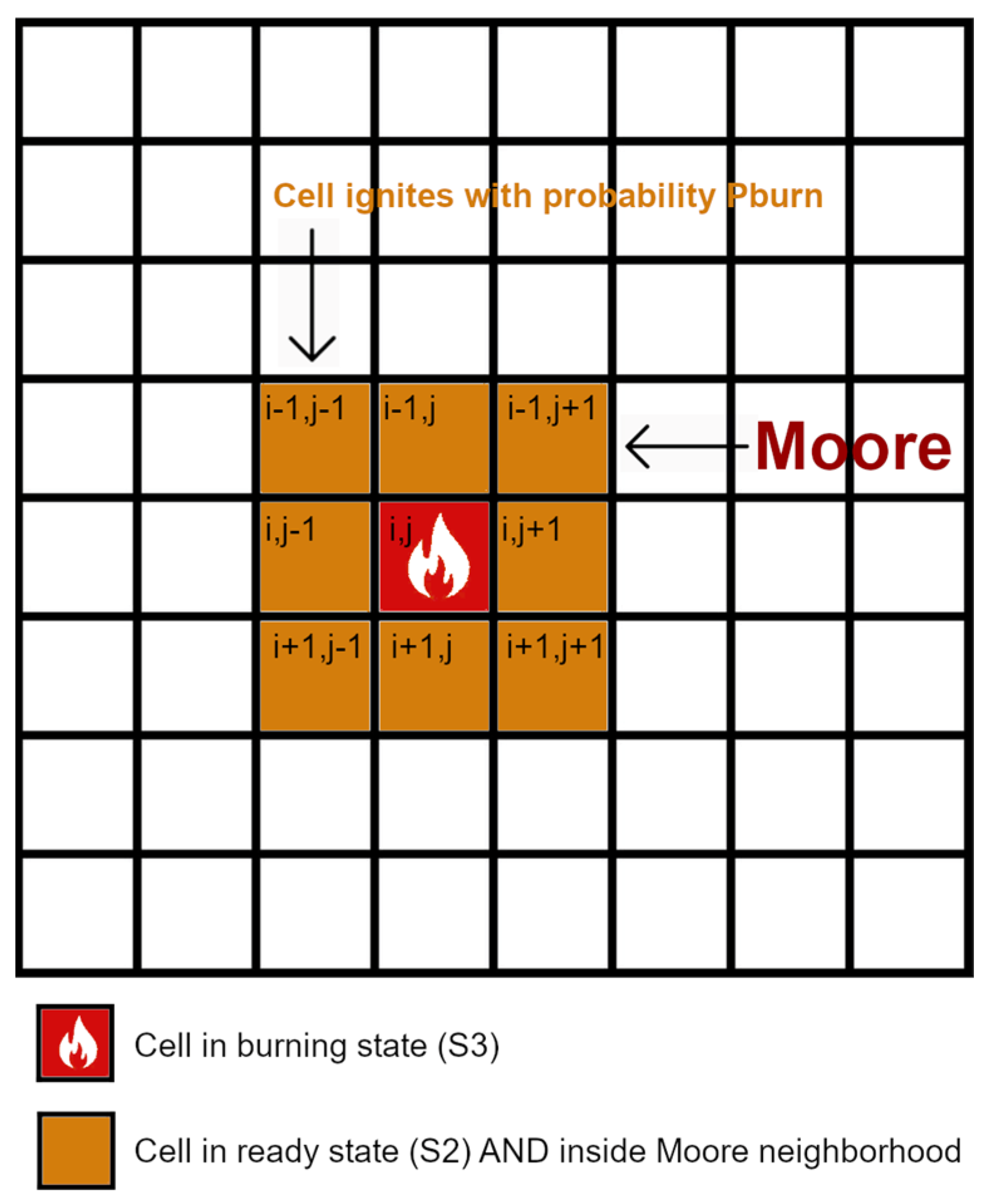
• A cell can be ignited (${\mathrm{S}}_3$) at the next iteration with probability P_burn (Figure 1) if one of its neighboring cells is burning (${\mathrm{S}}_3$) and the cell contains combustible fuel (${\mathrm{S}}_2$). Otherwise, it remains in state ${\mathrm{S}}_2$.
• A burned cell ($S_4$) has been completely consumed by the fire and cannot be reignited.
• Any changes in cell states occurring outside the defined discrete time steps of the simulation cannot be represented.

Figure 1. Moore neighborhood representation in a square lattice cellular automaton. Each cell neighboring an ignited cell (state S₃) is considered for ignition with probability $P_{burn}$, provided it contains combustible fuel (state S₂).

Figure 1. Moore neighborhood representation in a square lattice cellular automaton. Each cell neighboring an ignited cell (state S₃) is considered for ignition with probability $P_{burn}$, provided it contains combustible fuel (state S₂).

The probability $P_{burn}$ of a cell igniting at the next iteration can be calculated using Equation (2):

$$P_{burn} = P_0\left(1+P_{veg}\right)\left(1+P_{den}\right)P_w{P}_s{P}_m,$$

(2)

where $P_0$ is a base probability expressing the likelihood of a cell ignited by an adjacent one, under the influence of zero wind and no elevation difference. That probability is indirectly derived from a mathematical fire spread model (like the one proposed by Rothermel [16]) but since each vegetation type (fuel model) has different characteristics, the resulting rate of spread varies and cannot be represented by a single value. Hence, $P_0$ serves as a baseline representing the rate of spread under controlled conditions (no-wind and no-slope), while the remaining coefficients regulate the rate of spread according to the characteristics of the contained vegetation type and terrain.

$P_{veg}$ and $P_{den}$ are probability coefficients representing the type of the vegetation and its density, respectively, whose values are assigned through lookup tables parameterized according to the fuel type.

$P_w$ and $P_s$ denote probability coefficients associated with the influence of wind and terrain elevation on the propagation of fire, respectively. They can be calculated using Equations (3) and (4). Specifically, $P_w$ is given by

$$P_w=e^{\left[V\left(c_1+c_2\left(\mathit{cos}\left(\theta \right)-1\right)\right)\right]},$$

(3)

where c₁, c₂ are parameters, V is the wind velocity and θ is defined as the angle between the prevailing wind direction and the potential direction of fire spread. $P_s$ is given by

$$P_s=e^{a_s{\theta }_s}, {\mathsf{\theta }}_{\mathrm{s}}=\left\{\begin{array}{c}{\mathrm{t}\mathrm{a}\mathrm{n}}^{-1}\left({\displaystyle \frac{{\mathrm{E}}_1-{\mathrm{E}}_2}{\mathrm{l}}}\right) \mathrm{i}\mathrm{f} \mathrm{c}\mathrm{e}\mathrm{l}\mathrm{l}\mathrm{s} \mathrm{a}\mathrm{r}\mathrm{e} \mathrm{a}\mathrm{d}\mathrm{j}\mathrm{a}\mathrm{c}\mathrm{e}\mathrm{n}\mathrm{t}\\ {\mathrm{t}\mathrm{a}\mathrm{n}}^{-1}\left({\displaystyle \frac{{\mathrm{E}}_1-{\mathrm{E}}_2}{\mathrm{l}\sqrt{2}}}\right) \mathrm{i}\mathrm{f} \mathrm{c}\mathrm{e}\mathrm{l}\mathrm{l}\mathrm{s} \mathrm{a}\mathrm{r}\mathrm{e} \mathrm{d}\mathrm{i}\mathrm{a}\mathrm{g}\mathrm{o}\mathrm{n}\mathrm{a}\mathrm{l}\end{array}\right.,$$

(4)

where $a_s$ is a tunable parameter, ${\theta }_s$ represents the slope angle between the source (burning) cell and the target cell under consideration for fire propagation; l is the cell length, while $E_1$ and $E_2$ denote the elevations of the corresponding cell centroids.

Finally, $P_m$ is a probability coefficient representing the effect of the dead fuel moisture content—a significant factor influencing wildfire spread [17]—on fire propagation. $P_m$ is indirectly derived from a nonlinear regression model where the ROS is found to be exponentially related to the dead fuel moisture content [18]. A mathematical expression for $P_m$ based on the findings of [18] between the moisture content and the ROS is given in Equation (5):

$$P_m= {ae}^{-b{C}_m},$$

(5)

where $a,b$ are tunable user-specified parameters and $C_m$ is the dead fuel moisture content.

A well-known limitation of space and time discretization in cellular automata is that, at each iteration, a cell considered for ignition can exist only in a fully ignited state or remain completely unburned (in ${\mathrm{S}}_2$ state). Consequently, cases in which the fire front is expected to advance by a distance smaller than the cell size ($l_{cell}$) can only be represented probabilistically. Hence, the authors in [14] argue that the most appropriate way to express the constant probability term is as a function of the estimated ROS, as shown in Equation (6):

$$P_0\propto {\displaystyle \frac{R_{0}dt}{l_{cell}}},$$

(6)

where $R_0$ is a base estimation of ROS in m/min, $dt$ the duration of a simulation time step in minutes and $l_{cell}$ the length of the square cells in meters. Given that the term represents a probability, the simulation time step and cell size should be carefully selected accordingly.

2.2. A Crowdsourced Method for Simulating Wildfires

Methods based on crowdsourced data are not new in the field of civil protection and disaster management [1,19]. However, the fast-evolving, dynamic, and often unpredictable nature of emergency events creates significant challenges for the data acquisition of accurate situational data through conventional techniques. Usually, conventional data sources like remote sensing and drone aerial monitoring suffer from delays, limited spatial coverage, or infrastructure disruptions, particularly during the early phases of an incident.

In this context, harnessing the collective input of individuals located near the affected area becomes increasingly valuable since they can access raw data that are continuously updated and reflect the most current conditions on the ground. Several research attempts have highlighted the importance of data acquisition directly from raw user inputs, particularly for wildfire incidents [2,20]. Citizens can provide observations and estimations such as the fuel types, the wind speed, the exact ignition point or the advance of the fire front, through their mobile devices in almost real time. Since that particular data collection reflects the most current conditions in the field, it enables a wildfire simulator to generate even more accurate outputs based on that initialization. Additionally, in cases where uncertainty, rapid change, and limited access to conventional remote sensing sources exist, crowdsourced data sources are the only viable alternative to simulation initialization.

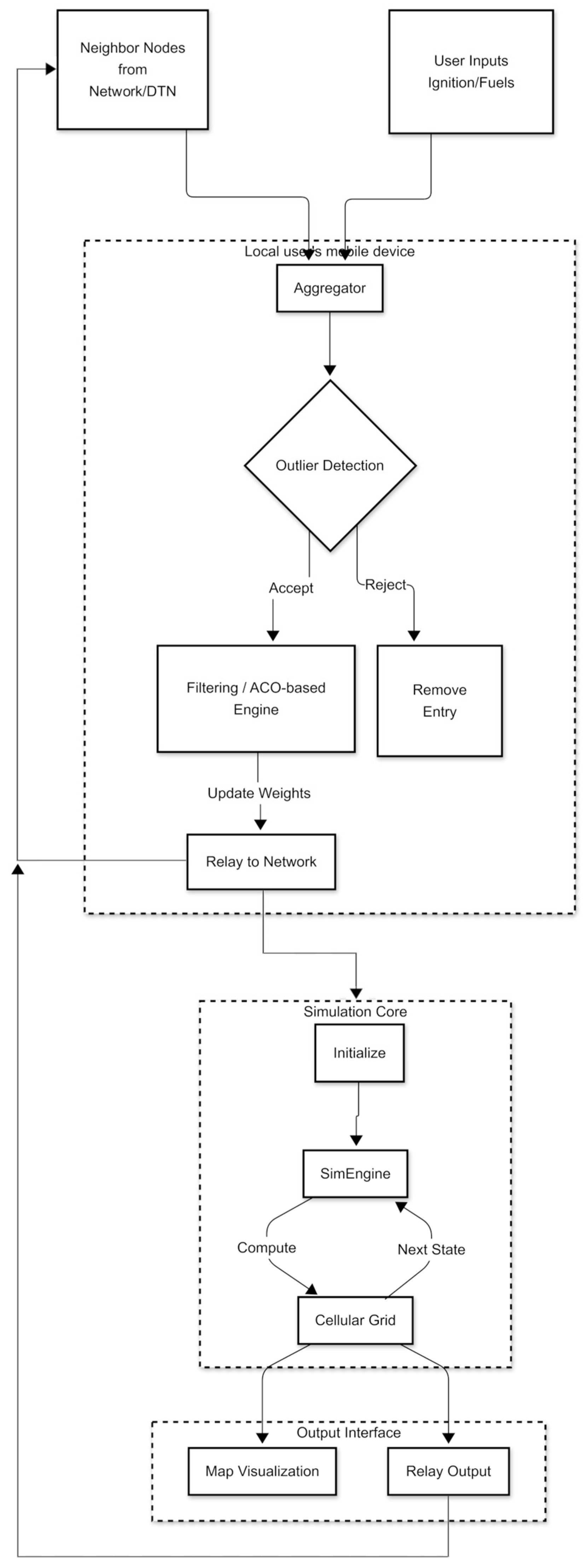
Based on the framework proposed in [2], we consider the setup shown in Figure 2, where individuals that eyewitness the spread of the wildfire report current conditions and in-field observations to nearby users via some type of network service (cellular, nearby communications, etc.). Subsequently, users can aggregate the collected information to fill gaps within their individual simulation domain, update previously known conditions, or validate existing data. Additional steps for data filtering and the resolution of ambiguous information may be applied as mentioned in [2]; however, these steps are omitted in the present study, as they would influence the simulation output in the test cases. The proposed methodology is applicable even in scenarios requiring a centralized wildfire simulator that is supplied with centrally managed input data (not necessarily crowdsourced). In such cases, the methodology enables the systematic examination of how variations in input data influence simulation outcomes.

2.3. Test Case

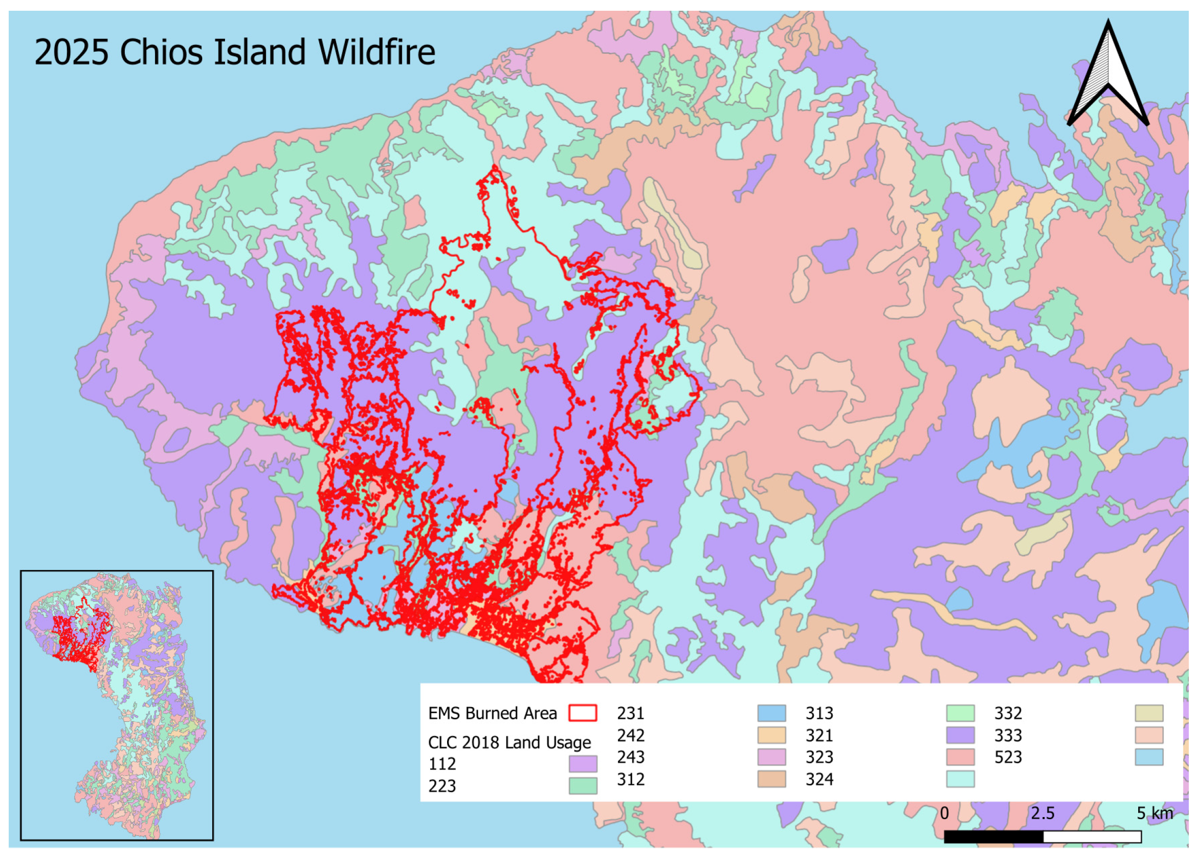
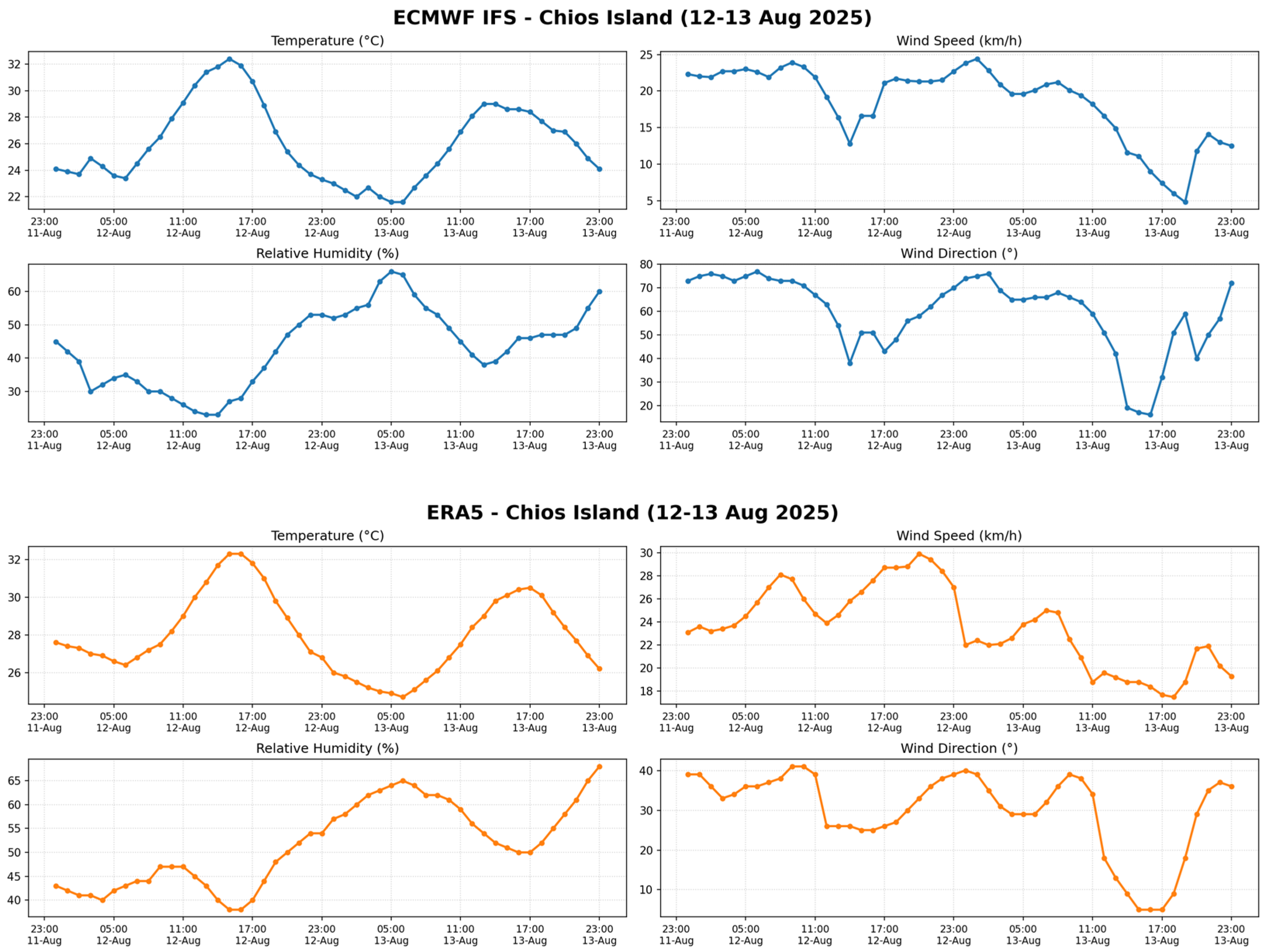
To evaluate the sensitivity of the simulation output to user inputs, the event of a wildfire in Chios Island was employed as a representative test case. On 12 August 2025 at 14:17 local time, a wildfire was reported on Chios Island, Greece, approximately 2 km north of the village of Nea Potamia near the Chalandra village. In response, the Copernicus Emergency Management Service (EMS) Rapid Mapping was activated to provide emergency mapping of the wildfire’s extent and associated damages, under activation ID EMSR834 [21]. According to the same EMS report, as of 15 August 2025, the wildfire had affected a total area of 6909 ha, as shown in Figure 3. During the incident, Chios Island was dominated by Meltemi (or Etesian) winds, a characteristic weather pattern of the Aegean Sea in July and August [22]. These strong, persistent, and dry winds consistently blew from the North or North-East (NNE) (Figure 4), creating conditions that significantly influenced fire behavior.

Due to the severity of the wildfire, authorities issued evacuation orders via the 112 emergency number for residents in the affected villages and surrounding areas, while evacuation and rescue efforts were conducted in parallel by the Hellenic Coast Guard. The wildfire spread through forestry, agricultural areas and near villages, damaging infrastructure, buildings and agricultural vegetated areas. Chios may experience significant long-term repercussions as a result of the wildfire, affecting the local economy and biodiversity, as well as the production of mastic and olive oil, sectors that constitute fundamental pillars of the island’s socio-economic and cultural fabric.

In the vicinity of that study area, we will attempt to run a series of simulation scenarios using meteorological data from the day of the event (Figure 4), along with forest fuel classification derived both from the extraction of data from the CLC 2018 dataset and from volunteer-based assessments, whereby participants manually indicate which areas should be assigned to each fuel class without relying on the spatial distribution suggested by the CLC dataset. Further details regarding the datasets and the applied methodology are provided in the following section.

2.4. Simulation Setup

In order to emulate the behavior of the crowdsourced dataset, we asked a group of volunteer firefighters to identify the fuel model they considered most appropriate for the simulation area, as well as the spatial extent of that particular fuel. As a baseline for comparison, we used the CORINE Land Cover (CLC) 2018 [23] (100 m resolution) dataset, after empirically aligning the spatial extent of the land use classes with their corresponding fuel model classification. As anticipated, discrepancies were observed between the spatial distribution of fuel types identified by field observers and those indirectly derived from the CLC dataset. This deviation is expected, as the CLC is designed for general land use and land cover mapping, rather than for forest fuel modeling. Consequently, its resolution differs from that of in-field observations. Furthermore, minor variations in land cover do not necessarily correspond to distinct fuel types from an operational firefighting perspective.

The weather conditions were obtained from the Open Meteo Historical Weather API [24], and used as a baseline with a selected resolution of 1 h (Figure 4). To assess the sensitivity of model inputs to different representations of atmospheric conditions, two alternative meteorological datasets available through the API were employed: the ECMWF Integrated Forecasting System (IFS) and the ERA5 reanalysis dataset. The IFS represents model-generated weather fields derived from the ECMWF’s numerical weather prediction system, while the ERA5 is an atmospheric reanalysis product, in which historical observations are assimilated into the same modeling framework to reconstruct past weather conditions. Then, we introduced some degree of small variation on the reported values to emulate the inherent variability and uncertainty commonly observed in crowdsourced originated datasets, thereby enhancing the realism of the simulation inputs (e.g., in cases where data from sensors were utilized). Topographic information regarding the elevation was acquired using data from the NASA Shuttle Radar Topography Mission (SRTM) at a 3-arc-second (~90 m) resolution.

To perform the simulation, we implemented the CA algorithm described in Section 2 using mainly JavaScript and other WEB technologies. This programming language was selected to ensure a purely client-side execution environment, facilitating cross-platform portability, with a specific focus on mobile devices. This architecture enables the deployment of the simulator directly in the field by operational firefighting personnel. Model parameters were defined based on a synthesis of the existing literature references, empirical observations, and iterative calibration derived from our specific knowledge of the simulated wildfire event.

Table 1. Parameterization and coefficient values utilized in the CA wildfire simulation model.

Parameter	Value	Parameter	Value
$P_0$ 1	0.741 2	$l_{cell}$	40.5 m
$c_1$	0.045	$a$	3.258
$c_2$	0.131	$b$	0.111
$a_s$	0.078	$dt$	10 min

¹ Calculated based on the dominant vegetation type of the simulation area. Refer to text for details. ² Different values used on each simulation based on the dataset provided by volunteer firefighters. Refer to text for details.

presents the specific values assigned to the model coefficients based on the notation used in [14].

A critical component of the simulation setup, following the methodology proposed by Alexandridis et al. [14], was the calibration of the base probability parameter $P_0$. To determine this value, we calculated the dominant vegetation type within the study area (CLC 321—Natural grassland), which can be mapped (based on additional observations of the area) to Fuel Model SH5 [25] as the reference metric. Using Rothermel’s model [16] under zero-slope and (near) zero-wind conditions, we calculated a baseline averaged rate of spread (ROS) of about 3 m/min for this vegetation class. Given a target temporal resolution $dt$ of 10 min, the optimal spatial resolution $l_{cell}$ was calculated to be approximately 40.5 m to maintain model stability, resulting in a $P_0$ value of 0.741.

We applied the same parameterization methodology to the three alternative vegetation datasets generated by the volunteer firefighter groups. The only difference lay in the classification approach: the groups directly mapped the areas (not the same as the CLC dataset) to the 40 standard fuel models, in addition to their CLC classes, rather than just assigning intermediate CLC codes, which are suboptimal for wildfire simulation. This approach (asking users to specify both CLC and Fuel Model codes) was chosen to enable future research into the accuracy of user-defined fuel model assignments within the context of wildfire simulation. The dominant land cover types identified in these scenarios were CLC 333 (Sparsely vegetated areas), CLC 321 (Natural grassland), and CLC 333. Based on the derived rate of spread (ROS) for these dominant classes (2.1, 3 and 2.1 m/min), the corresponding base probability values $P_0$ were calculated as 0.52, 0.741, and 0.52, respectively. ROS calculations were performed using the BehavePlus modeling software [26] as a guide. As the proposed approach is empirical, ROS values cannot be directly converted into quantitative probability coefficients. Consequently, model calibration through fine-tuning and experimental evaluation is required.

The $C_m$ value was estimated using Simard’s empirical regression model [27] for the calculation of the equilibrium moisture content (EMC). The EMC is a theoretical estimator of the fuel moisture content (FMC), based on historical environmental conditions such as precipitation, relative humidity, temperature, season of the year, etc. Assuming that the relative humidity during the incident (Figure 4) was fluctuating for the majority of the time between 10 and 50%, the EMC can be obtained using Equations (7) and (8) for the duration it exceeds 50%.

$$EMC=2.22749+0.160107\mathrm{H}-0.01478\mathrm{T}, 10\le H<50,$$

(7)

$$EMC=21.0606+0.005565H^2-0.0003505HT-0.483199H, 50\le H,$$

(8)

where $H$ is the relative humidity in percent and $T$ is the temperature in Fahrenheit. While Simard’s approach is widely used, the Van Wagner model [28] presents a viable alternative, alongside more recent developments, like those of Masinda et al. [29], which is based on experimental measurements.

Table 2. Correspondence between CLC 2018 land use classes and the probability coefficients applied in the CA model.

CLC Code	Type	Pden	Pveg
112	Discontinuous urban fabric	−0.5	−0.8
223	Olive groves	−0.3	−0.1
231	Pastures	−0.3	0.4
242	Complex cultivation patterns	0.1	0.1
243	Land principally occupied by agriculture, with significant areas of natural vegetation	0.25	0.5
312	Coniferous forest	0.35	0.7
313	Mixed forest	0.3	0.5
321	Natural grassland	0.3	0.4
323	Sclerophyllous vegetation	0.35	0.5
324	Transitional woodland/shrub	0.15	0.4
332	Bare rock	−1	−1
333	Sparsely vegetated areas	0	0.4
523	Sea and the ocean	−1	−1

illustrates the mapping between the CLC 2018 land cover classes and the corresponding fuel characteristic parameters utilized in the CA model we implemented.

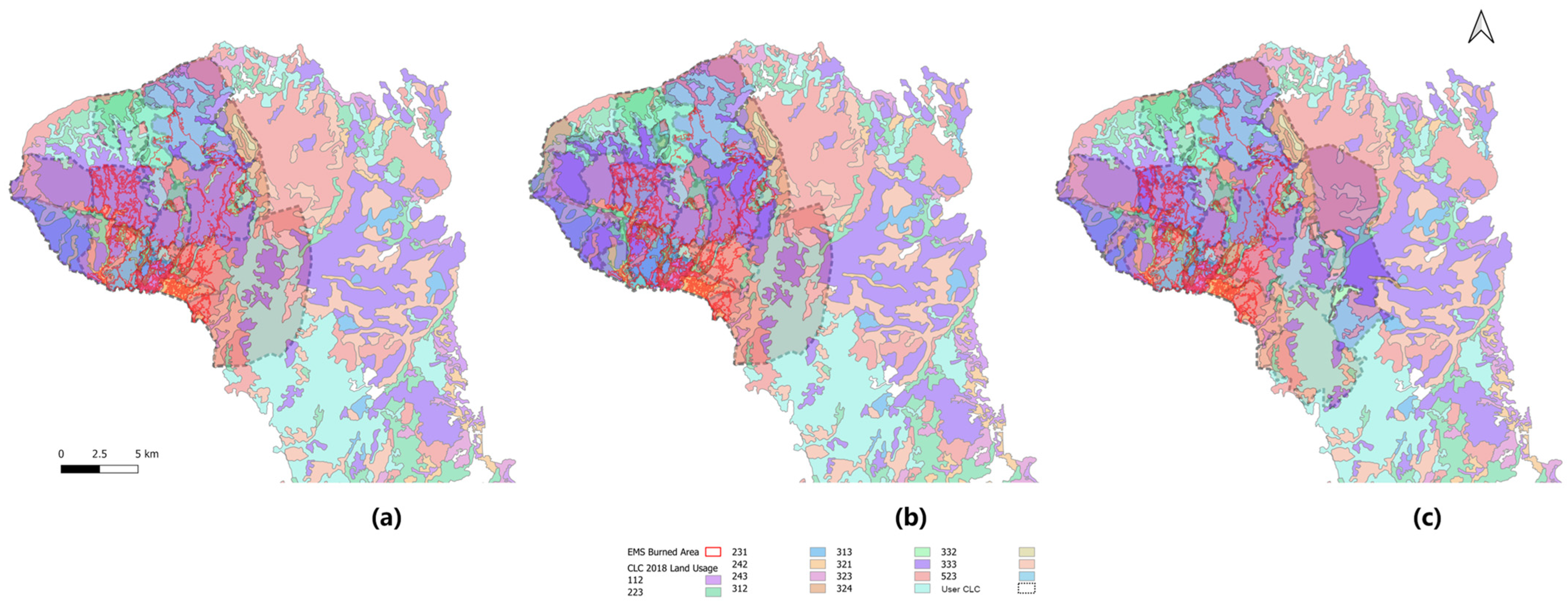
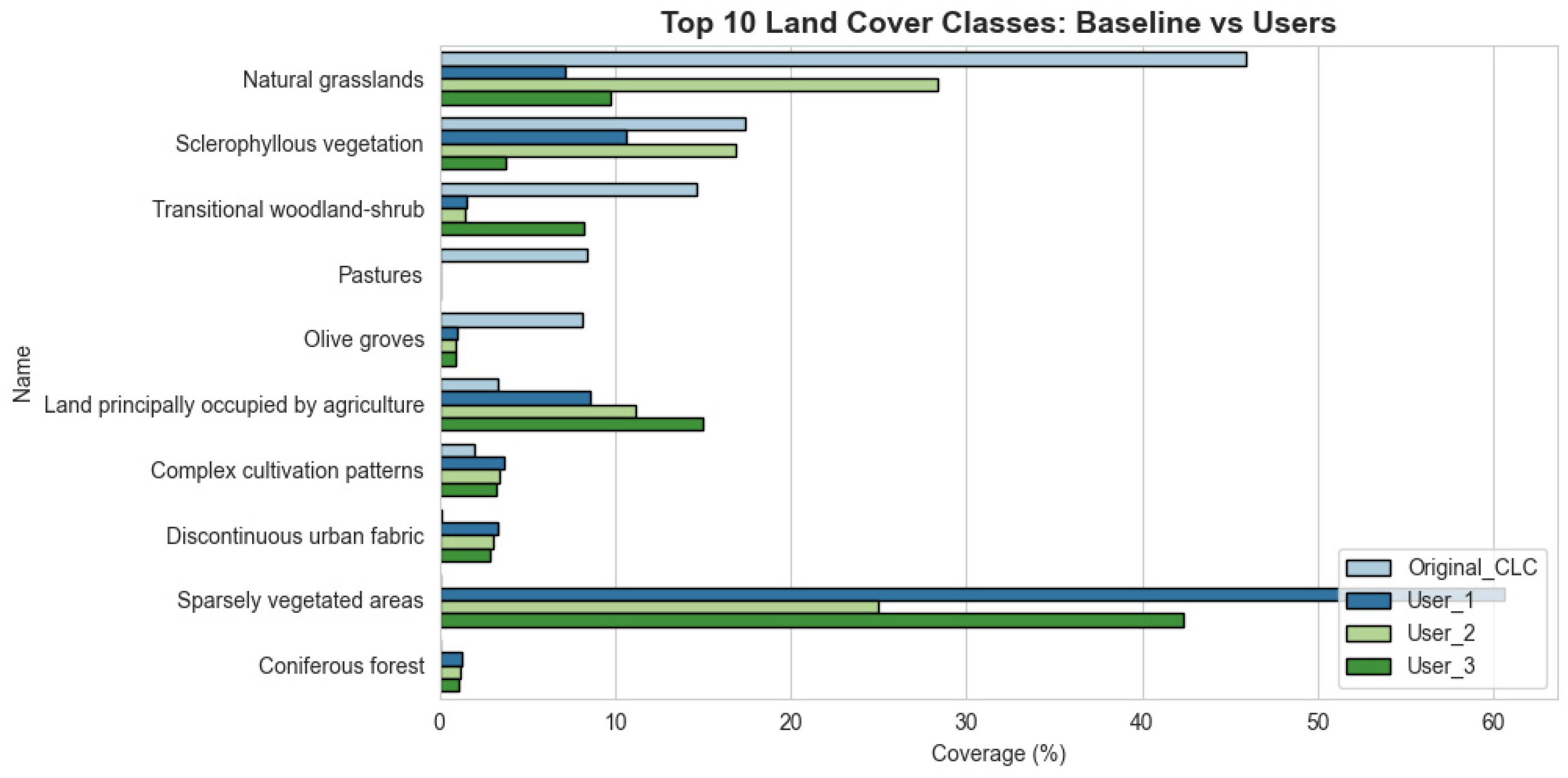
Figure 5 depicts the classification selections made by volunteer firefighter groups, projected alongside the CLC reference classes. A distinct trend toward geometric simplification is observable; volunteers consistently generalize the intricate CLC polygons. This behavior reflects a tendency to exclude non-essential fuel extents and to correct for discrepancies resulting from recent changes in land use. Additionally, Figure 6 shows the composition of land use coverage in the study area, using the burned area as a mask, comparing the baseline (CLC) with the estimates produced by the three volunteer user groups.

3. Results

It is evident from the weather graphs that the fire was wind-driven by strong NE Meltemi winds. The fire spread across a typical Greek island landscape, defined by mountainous terrain and heterogeneous fuel beds, making it even more difficult to accurately estimate its spread. We conducted a series of simulations using three weather datasets: the ECMWF IFS, ERA5 and a distorted version of the ERA5 dataset, against four datasets of fuels. The CLC classification is used as the primary (baseline) fuel dataset, with three additional fuel datasets produced by an equal number of volunteer firefighter groups.

3.1. Preprocessing of Raw Data

A methodological challenge encountered in this study concerns the spatial alignment of heterogeneous spatial datasets with differing resolutions and coordinate reference systems (CRSs). All input required resampling and reprojection to ensure consistency with the CA grid prior to simulation.

As mentioned, the fuel composition for the baseline run was derived from the CLC dataset (100 m spatial resolution), while topographic information was obtained from the NASA Shuttle Radar Topography Mission (SRTM) digital elevation model (90 m spatial resolution). In addition, alternative fuel composition scenarios were constructed using polygon features digitized by trained volunteers through the Google Earth 7.3 interface. A detailed description of the volunteer-based data acquisition and digitization workflow is provided in Appendix A.

At initialization, the CA simulator constructs a $N\times N$ grid covering the study area. For each grid cell, the centroid is computed in WGS 84 coordinates. The centroid is then transformed to the native coordinate reference system of each dataset to extract the corresponding environmental attributes. Categorical variables (fuel types from CLC and volunteer-defined polygons) were assigned using nearest-neighbor sampling based on the cell centroid location, preserving class integrity. Continuous elevation values from SRTM were interpolated to the CA grid using bilinear interpolation, from which the slope angle was subsequently derived. All spatial transformations and interpolations are performed only once during model initialization. After attribute assignment, the CA simulation operates exclusively on the internal grid representation, avoiding repeated resampling during runtime.

However, the resampling process introduces a systematic and spatially consistent approximation due to scale transformation. Since the interpolation is applied uniformly across the area, it does not introduce stochastic bias during propagation but rather reflects the intrinsic scale mismatch between available datasets and the selected grid size (l_cell). At the spatial scale considered in this study, this approximation is consistent with common practice in raster-based environmental modeling.

3.2. Simulation Runs

Although the observed fire on the island lasted approximately two days, the comparison is made with the simulated burned area after 24 h. From a strict methodological perspective, the durations are not identical; however, the 24 h simulation represents the most realistic timeframe for evaluating fire spread under the modeled conditions. We concluded that a longer simulation duration does not necessarily lead to better accuracy, since the introduced uncertainty of inputs will drift the estimated burned area further from the observed wildfire perimeter. Also, the firefighting actions are not modeled in that particular version of the model; therefore, their impact on the affected area cannot be represented by the simulation. Moreover, the final burned area morphology (Figure 3) supports this interpretation. In idealized conditions, wildfire spread tends toward an approximately elliptical shape. In the observed case, the final perimeter exhibits strong irregularities and directional discontinuities, consistent with suppression-driven containment and tactical interventions rather than purely physical spread processes. Extending the simulation beyond this period would substantially overestimate the burned area, as the model assumes uninterrupted fire spread in the absence of suppression or containment. This further justifies restricting the comparison to the initial propagation period.

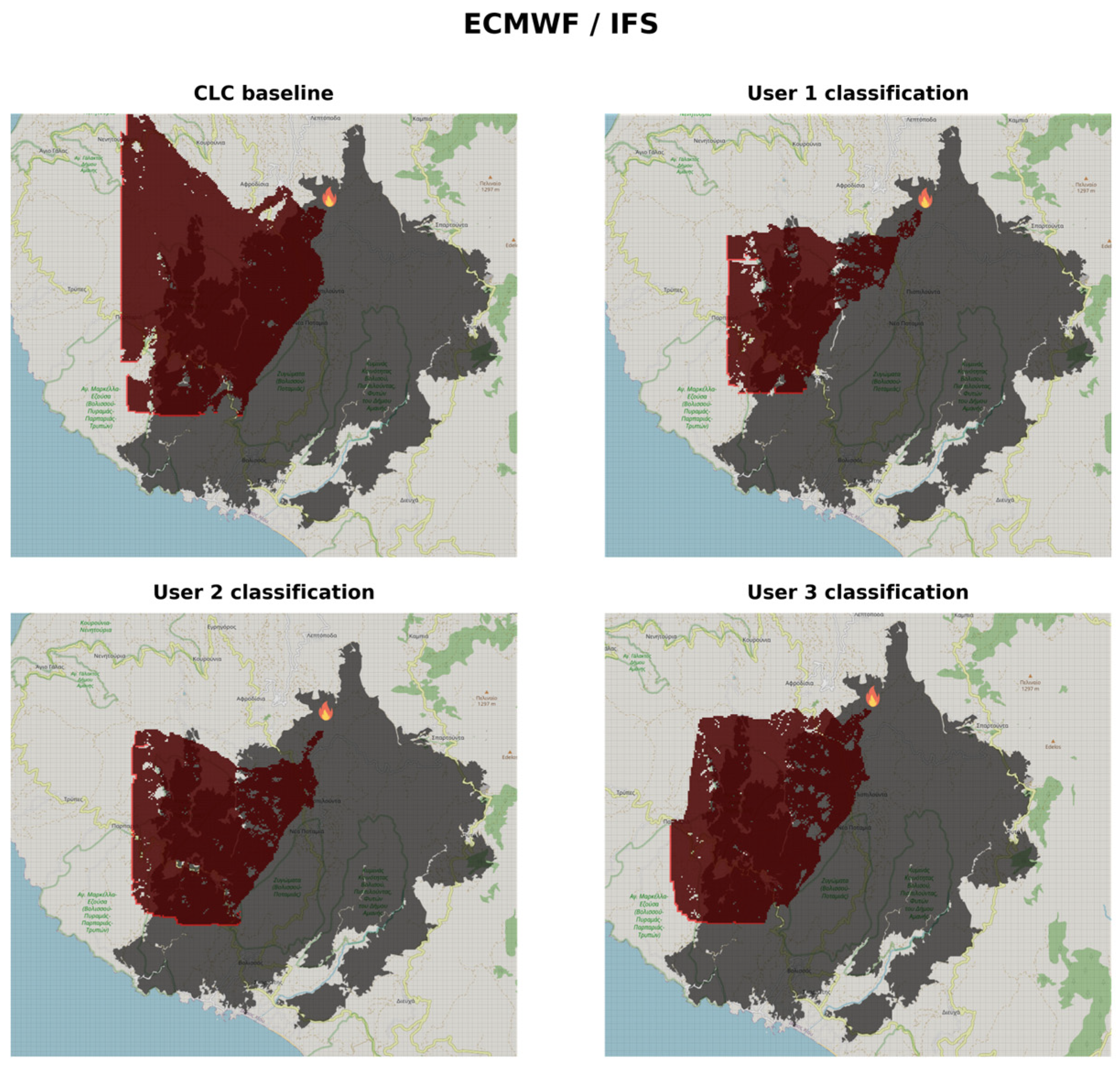
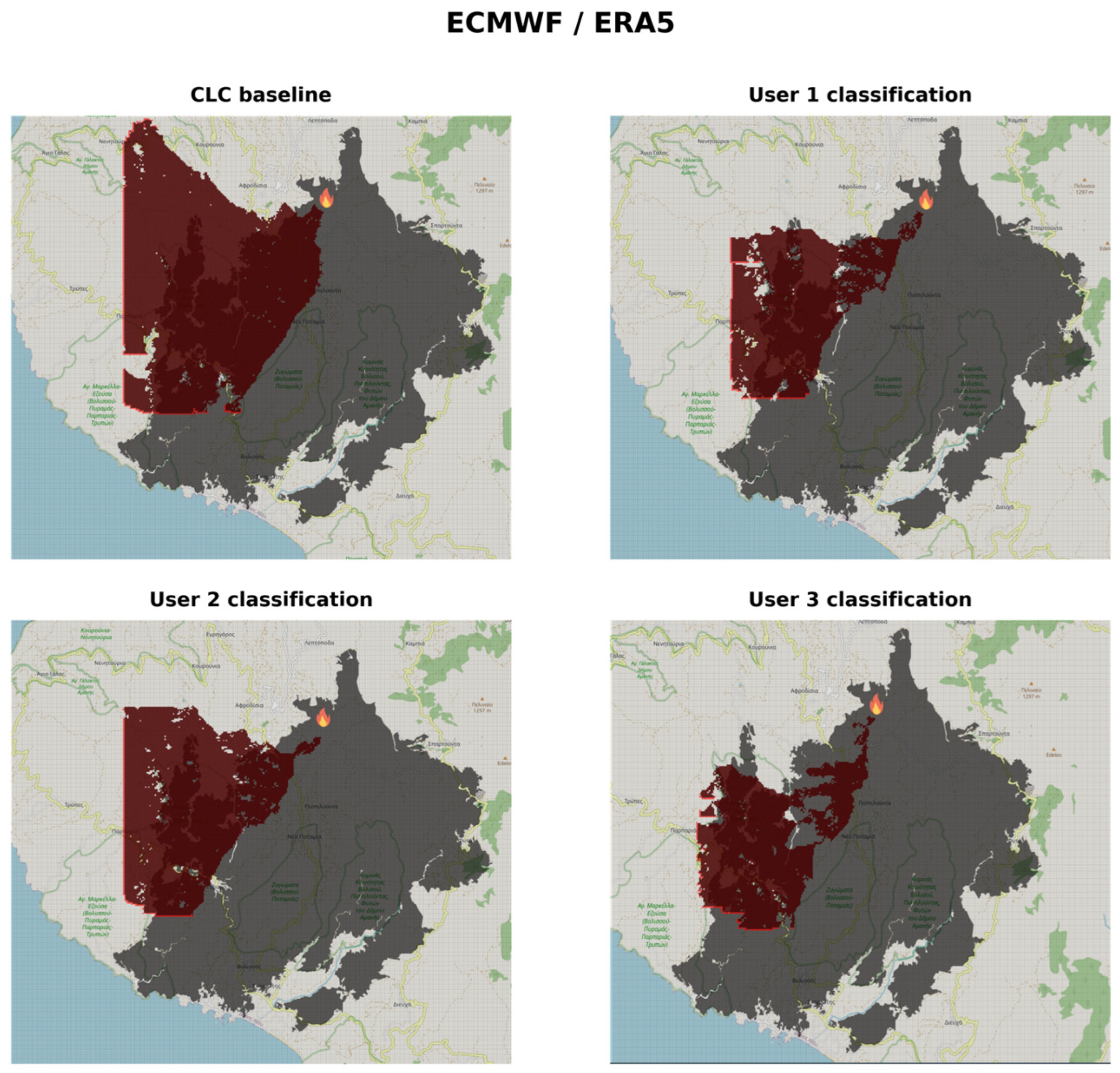
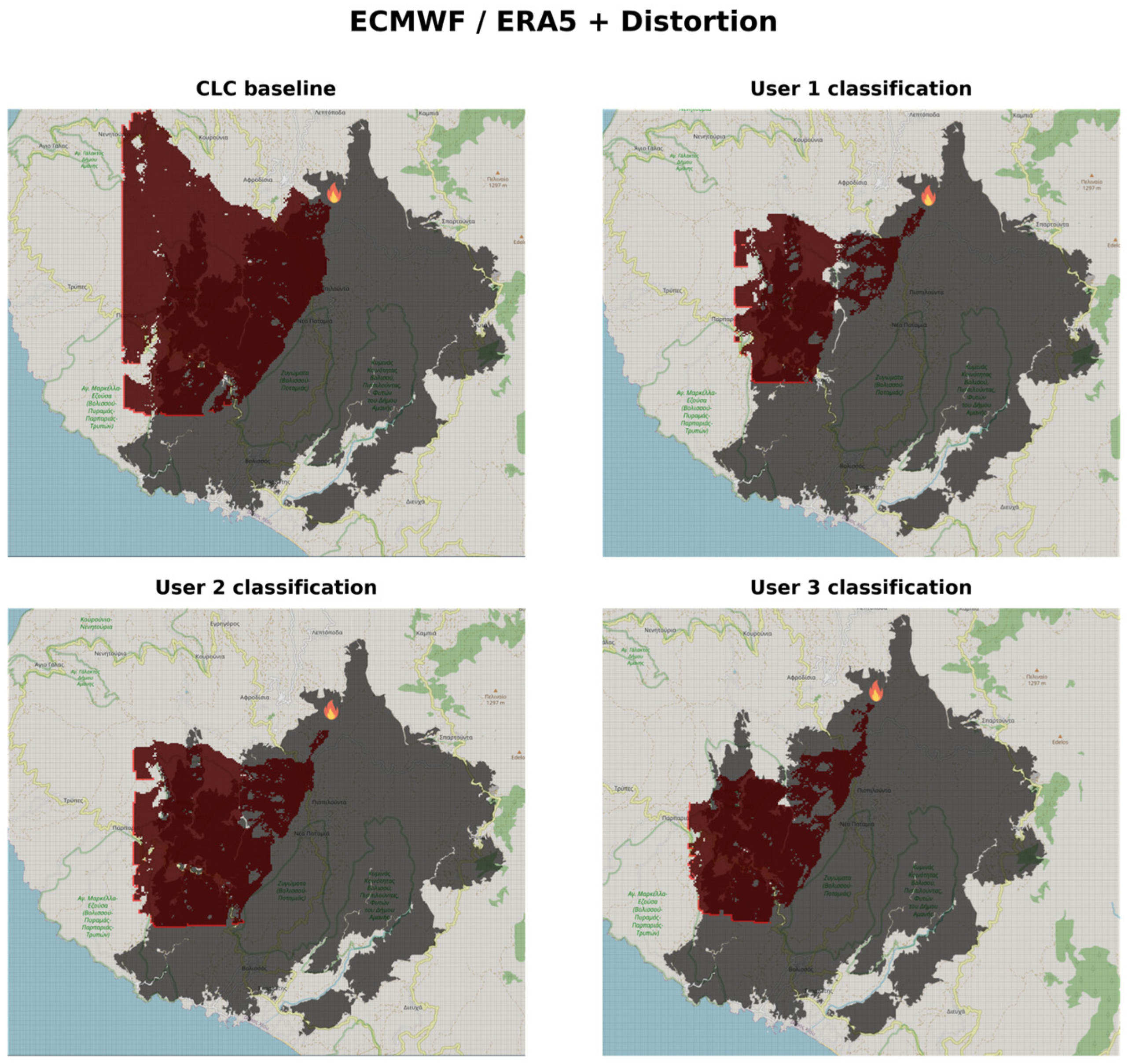
Figure 7, Figure 8 and Figure 9 illustrate the simulated wildfire spread obtained implementing the CA model using each meteorological dataset. For each figure, fire spread simulations are presented for four different fuel bed representations: the CLC baseline and three fuel maps derived from user classifications. The gray outline represents the observed wildfire perimeter at the time of the EMS mapping (2025-08-15 09:12 UTC), serving as a reference for model evaluation, while the red outline depicts the simulated fire perimeter after a 24 h simulation period.

This comparative visualization enables the assessment of how variations in meteorological conditions and fuel bed characterization influence the spatial extent and progression of the simulated wildfire spread.

Table 3. Simulated burned area for each configuration of meteorological and fuel bed datasets.

Weather Dataset	Fuel Dataset	Burned Area 1	Percent of Observed Burned Area 2
ECMWF IFS	CLC	3296 ha	47.76%
	User group 1	1482 ha	21.48%
	User group 2	2067 ha	29.96%
	User group 3	2410 ha	34.93%
ERA5	CLC	3242 ha	46.99%
	User group 1	1482 ha	21.48%
	User group 2	2122 ha	30.75%
	User group 3	1315 ha	19.06%
Distorted ERA5	CLC	3199 ha	46.36%
	User group 1	1225 ha	17.75%
	User group 2	1877 ha	27.20%
	User group 3	1361 ha	19.72%

¹ Simulated burned area in the first 24 h of the incident. ² Observed burned area as documented in EMSR834 report.

presents the total simulated burned area corresponding to each configuration of meteorological and fuel bed input datasets along with the percentage of the observed burned area calculated by each model.

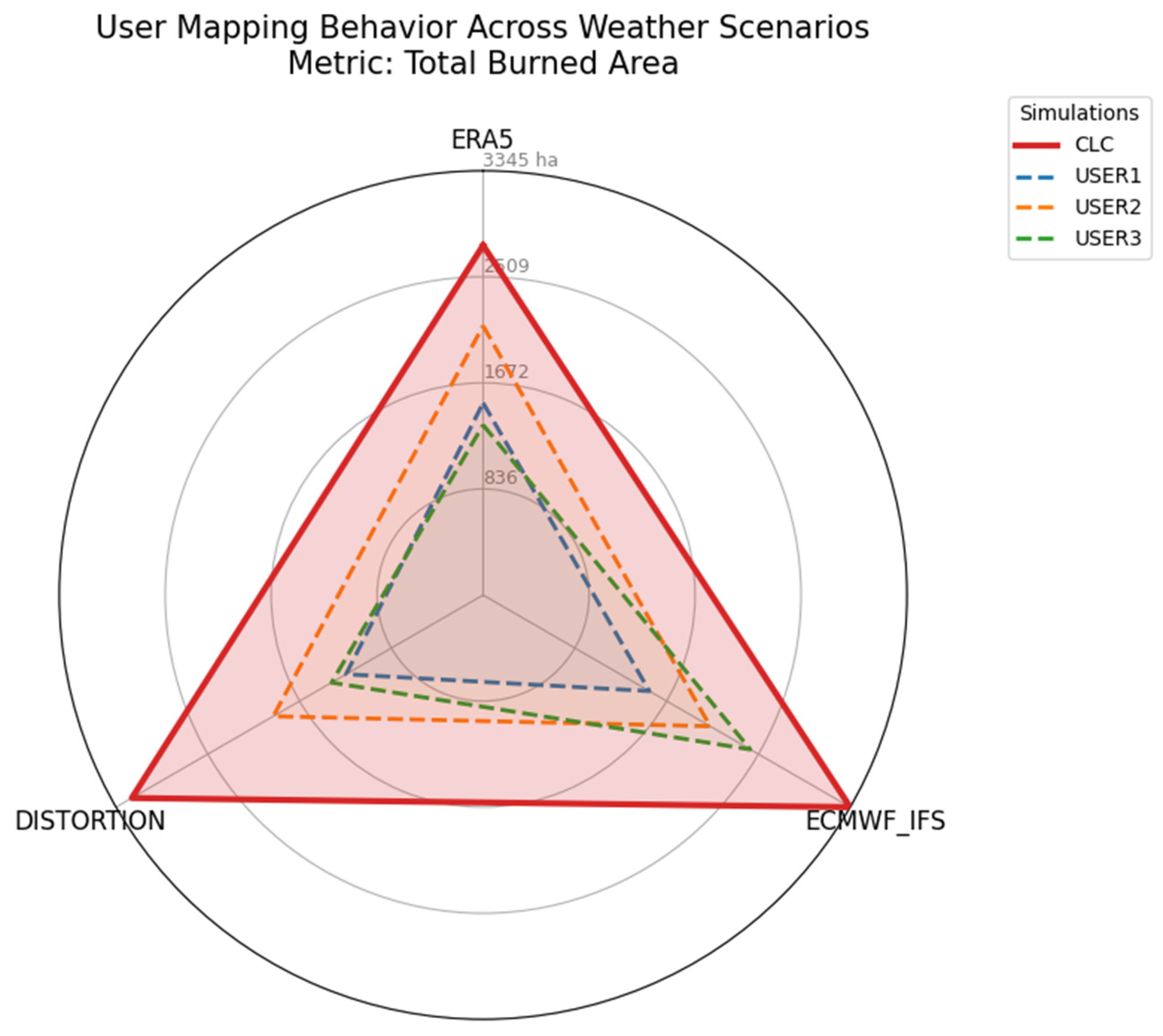
Examining the radar chart in Figure 10, which depicts the total simulated burned area (in hectares) across three distinct meteorological datasets (ERA5, ECMWF IFS, and a distorted weather scenario) for each of the four spatial fuel mappings (the standard CLC baseline and three independent volunteer datasets), we can conclude that

• The standard CLC baseline systematically overpredicts the total burned area compared to localized human mapping. Across all three meteorological scenarios, the baseline dataset yielded the largest simulated fire footprints. In contrast, all three user-defined fuel arrangements significantly constrained the fire spread, suggesting that the overrepresentation of the CLC 333 class (Figure 6) is a primary contributing factor.
• Certain user-defined fuel models suppress the influence of meteorological severity. It is evident that User 1 and User 2 exhibit “fuel-dominant” fire behavior, wherein the spatial arrangement of their fuels highly suppresses the fire’s response to weather.
• There are highly nonlinear interaction effects between specific fuel mappings and dynamic weather inputs. This is prominently illustrated by User 3. Under ERA5 and distorted weather conditions, User 3’s mapping behaves similarly to User 1, yielding heavily suppressed fire footprints.

4. Discussion

One of the most crucial parameters in a wildfire simulation is the weather, especially wind direction and speed. Because the data used in this study are synthetically generated by complex ECMWF models, rather than actual in-field observations, we cannot know the exact meteorological conditions close to the study area—which is characterized by mountainous terrain—which acts as an additional source of uncertainty. Moreover, land use information derived from data sources such as CLC 2018 can be employed only as a guide to forestry fuel classification. These datasets are aimed at general-purpose remote sensing applications; they were not originally designed to serve as fuel class representations.

The user-generated data sources were subject to personal and cognitive biases as the background of the participants was diverse. We observed a consistent overrepresentation of CLC 333 (Sparsely vegetated areas) across all three user groups. Given that these areas mainly contain grass and shrub fuels, we attribute this classification pattern to an operational bias: firefighters prioritize areas with significant tree density, often considering lower-density vegetation as less critical. Consequently, despite our methodological requirement for dual classification (Fuel Model Type and CLC code) to maintain consistency with the control dataset, users appeared to underestimate the significance of these lighter fuel types, defaulting to the “sparse” categorization. Given that the CA model is designed to be adaptable to any simulation area, we would typically either adjust the probability coefficients for these classes (refer to Table 2) or substitute certain areas with more appropriate classifications. However, neither approach was applied in this study, as our aim was to highlight the impact of the inputs rather than to fine-tune or overfit the model to a specific test case.

The implemented CA wildfire model incorporates stochastic transition rules to represent local variability in fire spread processes. However, this stochastic component does not necessarily imply that such models function as Monte Carlo frameworks [30] requiring repeated simulations to characterize statistical output distributions. In the present study, the CA model is not designed as a probabilistic simulator aimed at estimating the distributions of burned area. Instead, it operates as a scenario-based fire spread model: for a given set of environmental inputs (fuel distribution, topography, and meteorological conditions), the simulation produces a single realization of fire propagation. In practical applications, such as decision support during an active wildfire incident, the model would typically be executed once for a given configuration of environmental inputs to generate an estimation of fire spread under the given conditions. The objective is therefore not to generate a set of possible outcomes and select one of them, but rather to approximate the most plausible spread pattern given the specified environmental drivers. Furthermore, stochasticity in the model plays a secondary role relative to deterministic controls. Transition probabilities are strongly constrained by environmental factors such as wind, slope, and fuel type. Under dominant spread conditions, these probabilities approach unity, and the system behaves in a near-deterministic manner at the macroscopic scale. Consequently, variation in the random seed primarily influences small-scale perimeter irregularities rather than the overall burned area or the dominant direction of spread. The burned area metric reported in Table 3 therefore reflects the structural behavior of the model under the specified conditions rather than stochastic variability between runs.

5. Conclusions

It is hardly surprising that the simulation outputs are inevitably influenced by the limitations of the input data and the calibration of the parameters. What is not surprising are two observations of particular interest: Firstly, the model demonstrates high sensitivity to the initial inputs, leading to substantial divergence between configurations; secondly, distinct observers often attribute varying interpretations to the same land feature, even when possessing a shared theoretical and job background. Thus, the human element acts as a multiplier, which further amplifies the variability in the simulation results.

Finally, we can conclude that the tuning of the probability coefficients and the parameters in the models utilized in the CA model (such as the estimation of the EMC) may be more critical than originally assumed. We argue that a single coefficient configuration cannot be universally applicable, considering the wide variety of landscapes, weather conditions and fuel bed compositions. The high complexity of the underlying physical phenomena cannot be adequately captured by a limited, static set of parameters; therefore, precise, case-specific tuning is essential. From an operational standpoint, requiring end users with no forestry or fire science expertise to manually select appropriate parameter configurations is not a realistic assumption. This limitation outlines a new area for further study, regarding the optimization of site-specific configurations.

Parameter tuning constitutes a critical component of CA-based models, as model performance strongly depends on the appropriate calibration of their coefficients. However, as the findings of this paper indicate, expecting end users to manually calibrate these parameters across diverse configuration scenarios—such as varying weather conditions, fuel types, and landscape characteristics—is unrealistic and often impractical. As future work, we propose the development of an automated parameter tuning algorithm based on the Ant Colony Optimization (ACO) metaheuristic (or any other optimization technique meeting the time constraints of our environment), aimed at dynamically adapting model coefficients in near-real time, thereby alleviating the need for manual calibration by end users.

References

1. Mazzoleni, M.; Verlaan, M.; Alfonso, L.; Monego, M.; Norbiato, D.; Ferri, M.; Solomatine, D.P. Can assimilation of crowdsourced data in hydrological modelling improve flood prediction? Hydrol. Earth Syst. Sci. 2017, 21, 839–861. [Google Scholar] [CrossRef]
2. Karakonstantis, I.; Xylomenos, G. Improving Wildfire Simulations via Geometric Primitive Analysis in Noisy Crowdsourced Data. Appl. Sci. 2025, 15, 8844. [Google Scholar] [CrossRef]
3. Ménard, A.; Marceau, D.J. Exploration of Spatial Scale Sensitivity in Geographic Cellular Automata. Environ. Plan. B Plan. Des. 2005, 32, 693–714. [Google Scholar] [CrossRef]
4. Anstett-Collin, F.; Goffart, J.; Mara, T.; Denis-Vidal, L. Sensitivity analysis of complex models: Coping with dynamic and static inputs. Reliab. Eng. Syst. Saf. 2015, 134, 268–275. [Google Scholar] [CrossRef]
5. Alexandridis, A.; Vakalis, D.; Siettos, C.I.; Bafas, G.V. A cellular automata model for forest fire spread prediction: The case of the wildfire that swept through Spetses Island in 1990. Appl. Math. Comput. 2008, 204, 191–201. [Google Scholar] [CrossRef]
6. Freire, J.G.; DaCamara, C.C. Using cellular automata to simulate wildfire propagation and to assist in fire management. Nat. Hazards Earth Syst. Sci. 2019, 19, 169–179. [Google Scholar] [CrossRef]
7. Ghisu, T.; Arca, B.; Pellizzaro, G.; Duce, P. An optimal Cellular Automata algorithm for simulating wildfire spread. Environ. Model. Softw. 2015, 71, 1–14. [Google Scholar] [CrossRef]
8. Karafyllidis, I.; Thanailakis, A. A model for predicting forest fire spreading using cellular automata. Ecol. Model. 1997, 99, 87–97. [Google Scholar] [CrossRef]
9. Velasquez, W.; Munoz-Arcentales, A.; Bohnert, T.M.; Salvachua, J. Wildfire Propagation Simulation Tool using Cellular Automata and GIS. In 2019 International Symposium on Networks, Computers and Communications (ISNCC); IEEE: Istanbul, Turkey, 2019; pp. 1–7. [Google Scholar]
10. Xiao, X.; Wang, P.; Chou, K.-C. Cellular Automata and Its Applications in Protein Bioinformatics. Curr. Protein Pept. Sci. 2011, 12, 508–519. [Google Scholar] [CrossRef] [PubMed]
11. Rollier, M.; Zielinski, K.M.C.; Daly, A.J.; Bruno, O.M.; Baetens, J.M. A comprehensive taxonomy of cellular automata. Commun. Nonlinear Sci. Numer. Simul. 2025, 140, 108362. [Google Scholar] [CrossRef]
12. Karakonstantis, I.; Xylomenos, G. A Review of Two-Dimensional Cellular Automata Models for Wildfire Simulation: Methods, Capabilities, and Limitations. Fire 2026, 9, 108. [Google Scholar] [CrossRef]
13. Trunfio, G.A.; D’Ambrosio, D.; Rongo, R.; Spataro, W.; Di Gregorio, S. A New Algorithm for Simulating Wildfire Spread through Cellular Automata. ACM Trans. Model. Comput. Simul. 2011, 22, 6. [Google Scholar] [CrossRef]
14. Alexandridis, A.; Russo, L.; Vakalis, D.; Bafas, G.V.; Siettos, C.I. Wildland fire spread modelling using cellular automata: Evolution in large-scale spatially heterogeneous environments under fire suppression tactics. Int. J. Wildland Fire 2011, 20, 633. [Google Scholar] [CrossRef]
15. Hernández Encinas, L.; Hoya White, S.; Martín Del Rey, A.; Rodríguez Sánchez, G. Modelling forest fire spread using hexagonal cellular automata. Appl. Math. Model. 2007, 31, 1213–1227. [Google Scholar] [CrossRef]
16. Rothermel, R.C. A Mathematical Model for Predicting Fire Spread in Wildland Fuels; INT-115; USDA Forest Service, Intermountain Forest and Range Experiment Station: Odgen, UT, USA, 1972.
17. Matthews, S. Dead fuel moisture research: 1991–2012. Int. J. Wildland Fire 2014, 23, 78–92. [Google Scholar] [CrossRef]
18. Martins Fernandes, P.A. Fire spread prediction in shrub fuels in Portugal. For. Ecol. Manag. 2001, 144, 67–74. [Google Scholar] [CrossRef]
19. Steed, R.J.; Fuenzalida, A.; Bossu, R.; Bondár, I.; Heinloo, A.; Dupont, A.; Saul, J.; Strollo, A. Crowdsourcing triggers rapid, reliable earthquake locations. Sci. Adv. 2019, 5, eaau9824. [Google Scholar] [CrossRef] [PubMed]
20. Zhong, X.; Duckham, M.; Chong, D.; Tolhurst, K. Real-time estimation of wildfire perimeters from curated crowdsourcing. Sci. Rep. 2016, 6, 24206. [Google Scholar] [CrossRef] [PubMed]
21. EMSR834 Wildfire in the Municipality of Chios. 2025. Available online: https://civilprotection.gov.gr/copernicus/2025-emsr834-pyrkagia-ston-dimo-hioy (accessed on 1 March 2026).
22. Ruffault, J.; Curt, T.; Moron, V.; Trigo, R.M.; Mouillot, F.; Koutsias, N.; Pimont, F.; Martin-StPaul, N.; Barbero, R.; Dupuy, J.-L.; et al. Increased likelihood of heat-induced large wildfires in the Mediterranean Basin. Sci. Rep. 2020, 10, 13790. [Google Scholar] [CrossRef] [PubMed]
23. European Environment Agency (EEA). Corine Land Cover 2018 (CLC 2018) Dataset. 2019. Available online: https://land.copernicus.eu/en/products/corine-land-cover (accessed on 1 March 2026).
24. Historical Weather API. Open-Meteo. 2023. Available online: https://open-meteo.com/en/docs/historical-weather-api (accessed on 5 January 2026).
25. Scott, J.H.; Burgan, R.E. Standard Fire Behavior Fuel Models: A Comprehensive Set for Use with Rothermel’s Surface Fire Spread Model; U.S. Department of Agriculture, Forest Service, Rocky Mountain Research Station: Ft. Collins, CO, USA, 2005.
26. Andrews, P.; Bevins, C.; Seli, R. BehavePlus Fire Modeling System, Version 4.0: User’s Guide. General Technical Report, RMRS-GTR-106WWW Revised; USDA Forest Service, Rocky Mountain Research Station: Ogden, UT, USA, 2008. [Google Scholar]
27. Simard, A.J. The Moisture Content of Forest Fuels—I: A Review of the Basic Concepts; Government of Canada, Department of Forestry and Rural Development, Forest Fire Research Institute: Ottawa, ON, Canada, 1968.
28. Van Wagner, C.E.; Pickett, T.L. Equations and FORTRAN Program for the Canadian Forest Fire Weather Index System; Canadian Forestry Service, Petawawa National Forestry Institute: Chalk River, ON, Canada, 1985.
29. Masinda, M.M.; Li, F.; Liu, Q.; Sun, L.; Hu, T. Prediction model of moisture content of dead fine fuel in forest plantations on Maoer Mountain, Northeast China. J. For. Res. 2021, 32, 2023–2035. [Google Scholar] [CrossRef]
30. Graham, C.; Talay, D. Stochastic Simulation and Monte Carlo Methods: Mathematical Foundations of Stochastic Simulation. In Stochastic Modelling and Applied Probability; Springer: Berlin/Heidelberg, Germany, 2013; Volume 68. [Google Scholar]
Figure 2. Flowchart of a decentralized wildfire simulator that utilizes crowdsourced data, as proposed in [2]. Simulation results are influenced by user decision-making, depending on how environmental conditions and fuel properties are reported.
Information 17 00289 g002
Figure 3. Burned area on Chios Island, Greece, as documented in Copernicus EMS Rapid Mapping activation EMSR834 (2025) [21]. Map created using CLC 2018 land usage data from [23] and QGIS 3.40 software.
Information 17 00289 g003
Figure 4. Meteorological conditions for the affected region during 12−13 August 2025. Data retrieved from the Open-Meteo Historical Weather API. Charts shown in blue correspond to ECMWF IFS, whereas those in orange correspond to ERA5.
Information 17 00289 g004
Figure 5. Classification near the burned area (red outline) of the wildfire as determined by three separate groups of volunteer firefighters (maps (a), (b), and (c), respectively). CLC code mapping consistent with the previous map; user classification is indicated by the black dotted outline as shown in the map legend.
Information 17 00289 g005
Figure 6. Top 10 land use classes within the study area based on user classification.
Information 17 00289 g006
Figure 7. Simulated wildfire spread on study areausing IFS with four fuel bed representations. Gray outline: observed fire perimeter; red outline: simulated spread at 24 h. All maps include toponyms in Greek which are irrelevant for our analysis.
Information 17 00289 g007
Figure 8. Simulated wildfire spread on study area using ERA5 with four fuel bed representations. Gray outline: observed fire perimeter; red outline: simulated spread at 24 h.
Information 17 00289 g008
Figure 9. Simulated wildfire spread on study area using slightly distorted ERA5 weather data with four fuel bed representations. Gray outline: observed fire perimeter; red outline: simulated spread at 24 h.
Information 17 00289 g009
Figure 10. Sensitivity of simulated fire extent to weather conditions and fuel mapping source. The CLC baseline consistently overpredicts burned area compared to user mappings. Notably, the graph highlights strong interaction effects, such as User 3’s extreme vulnerability to ECMWF IFS weather inputs compared to their otherwise suppressed fire behavior.
Information 17 00289 g010