Article

Knowledge-Based Design Methodology for Human Resources Information Management

by
Sofía Morales-Zaleta
,
Mirna Patricia Ponce-Flores
*,
Guadalupe Castilla-Valdez
,
Juan Frausto-Solís
,
Juan Javier González Barbosa
* and
Erika Alarcón-Ruiz
División de Estudios de Posgrado e Investigación, Tecnológico Nacional de México/Instituto Tecnológico de Ciudad Madero, Ciudad Madero 89440, Mexico
*
Authors to whom correspondence should be addressed.
Information 2026, 17(3), 279; https://doi.org/10.3390/info17030279
Submission received: 31 December 2025 / Revised: 23 February 2026 / Accepted: 2 March 2026 / Published: 11 March 2026
(This article belongs to the Section Information Systems)

Abstract

Human resource management is a strategic axis for organizations, especially in contexts where artificial intelligence (AI) tools, such as natural language processing (NLP), play a fundamental role. Recruiting external applicants from large CV repositories requires consistent screening. The proposed methodology involves leveraging an existing curriculum vitae (CV) repository, structuring and indexing the data within a vector-based knowledge base, and applying retrieval techniques to identify candidates that satisfy role-specific criteria. Using 5029 CVs as benchmarks, we evaluate 3 queries, 3 variables (Degree, Skills, Experience), and 7 scenarios. Sampling n = 76 CVs for Queries 1–2 and n = 350 CVs for Query 3. The proposed approach achieved consistently high specificity across scenarios and query profiles, while sensitivity showed the largest fluctuations, particularly under single-requirement configurations. Across all queries and scenarios, accuracy ranged 65.79–98.00%, specificity 86.67–100.00%, and sensitivity 0.00–94.92%, while error rates decreased from 34.21% to 2.00% as constraint strictness increased. Sensitivity fluctuated most under single-requirement settings, and Experience-only screening showed the weakest selection behavior. Moreover, the results indicate that the ability to confirm suitable candidates is sensitive to query formulation, since non-standard role naming, experience phrasing, and other lexical variations can reduce the system’s capacity to detect positive evidence. Overall, these findings indicate that a knowledge-base-centered design enables consistent and interpretable requirement-driven candidate screening and provides a quantitative baseline for future improvements in recruitment-oriented retrieval systems.

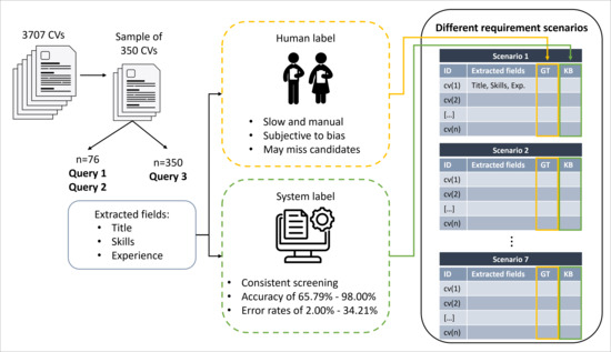
Graphical Abstract

1. Introduction

Human resource management is strategic for the success of organizations. The proper management of talent has always been a key factor, especially in contexts of globalization and rapid technological growth [1]. In recent years, the human resource landscape has begun to transform with the incorporation of new technologies and the accelerated digital transformation of its processes [2]. However, many companies still rely heavily on manual personnel management processes, which can be inefficient, time-consuming, difficult to update, and prone to errors [2,3].
Talent recruitment, a critical function within human resource management, has traditionally relied on manual screening carried out by designated personnel to identify qualified candidates [1,4]. However, this method has become increasingly inadequate in a rapidly evolving labor market. The high volume of applications submitted for each job posting, the growing complexity of candidate information, and the diversification of current data sources often result in recruiters processing only a fraction of the received applications, leading to the loss of potentially suitable candidates [1,2,4].
To meet these challenges, it is necessary to reinvent recruitment methods through digital systems and automation. This paper proposes a knowledge-based design methodology for managing and retrieving applicant information in human resource contexts through a retrieval-based framework. The study focuses on organizing CV information in a vector database using ChromaDB (Chroma, San Francisco, CA, USA) to enable semantic retrieval under predefined recruitment requirements, integrating information extraction, embedding generation, metadata construction, and semantic retrieval to support candidate selection under varying constraint scenarios. The screening process is driven by three job-profile queries (Query 1–Query 3), which represent different formulations of recruitment requirements and allow assessing sensitivity to query wording. The evaluation analyzes system performance across multiple logical combinations of recruitment requirements using confusion matrices and the derived metrics.
The remainder of this paper is organized as follows. Section 2 presents the materials used in this study, including a description of the dataset, the computational environment in which the experiments were conducted, and the main concepts required to interpret the evaluation (e.g., accuracy, specificity, sensitivity, precision, error rate, and the confusion matrix). Section 3 describes the proposed method, detailing each stage of the knowledge-based workflow, from document processing and knowledge base construction to query formulation and retrieval. Section 4 reports the results obtained from the evaluation scenarios and includes the statistical tests used to analyze differences across scenarios and queries. Section 5 provides the discussion of the findings and their implications, and outlines future research directions motivated by the observed system behavior. Finally, Section 6 presents the conclusions of the study.

2. Materials

This section describes the materials used to conduct the experimental evaluation of the proposed methodology. It includes a description of the dataset employed in the study, the computational environment in which the experiments were performed, and the evaluation metrics adopted to assess system performance. In addition, the section introduces the key concepts required to interpret the results, including precision, error rate, and the confusion matrix. Together, these elements provide the necessary context for understanding the methodological choices and the experimental outcomes presented in the following sections.

2.1. Dataset

This study used an annotated curriculum vitae (CV) dataset obtained from publicly available repositories on Kaggle (Kaggle Inc., San Francisco, CA, USA) [5] and Hugging Face (Hugging Face Inc., New York, NY, USA) [6]. The dataset consists of PDF-formatted CVs annotated for named entity recognition (NER), covering key information typically found in recruitment documents, such as personal data, skills, education, professional experience, and certifications.
The CVs represent a wide range of professional domains, including technical and non-technical fields, reflecting the diversity of real-world applicant profiles. The data was collected from 1 to 18 March 2025 with a screening process to ensure formatting and completeness of information such as personal data, skills, education, experience, and certifications [5,6,7].
The repositories contain a total of 5029 CV records. Each record is distributed as a JSON file that includes the extracted CV text and its NER annotations, typically organized into two main fields: text (the CV content) and annotations (a list of labeled spans).
To clarify the structure of the annotated CV records used in this study, Box 1 presents a simplified excerpt of a JavaScript Object Notation (JSON) sample from the dataset repositories. Each record contains the raw text extracted from a PDF CV and an annotations field storing the labeled spans as triplets of start index, end index, and entity label.
Box 1. Example JSON record excerpt from the annotated CV dataset (simplified).
{
“text”: “One97 Communications Limited\nData Scientist Jan 2019 to Till Date\nDetect important information from images and redact required fields. YOLO CNN Object-detection, OCR\nInsights, find anomaly or performance drop in all possible sub-space.\nPredict the Insurance claim probability. Estimate the premium amount to be charged\nB.Tech (Computer Science) from SGBAU university in 2017.\nM.Tech (Computer Science Engineering) from Indian Institute of Technology (IIT), Kanpur in 2019\nWORK EXPERIENCE\nEDUCATION\nMACY WILLIAMS\nDATA SCIENTIST\nData Scientist working on problems related to market research and customer analysis. I want to expand my arsenal of\napplication building and work on different kinds of problems. Looking for a role where I can work with a coordinative team\nand exchange knowledge during the process.\nJava, C++, Python, Machine Learning, Algorithms, Natural Language Processing, Deep Learning, Computer Vision, Pattern\nRecognition, Data Science, Data Analysis, Software Engineer, Data Analyst, C, PySpark, Kubeflow.\nABOUT\nSKILLS\nCustomer browsing patterns.\nPredict potential RTO (Return To Origin) orders for e-commerce.\nObject Detection.\nPROJECTS\nACTIVITES”,
“annotations”: [
[30, 44, “SKILL: Data Scientist”],
[194, 205, “SKILL: performance”],
[442, 452, “SKILL: Technology”],
[657, 665, “SKILL: Building”],
[781, 790, “SKILL: Knowledge”],
[811, 815, “SKILL: java”],
[822, 828, “SKILL: python”],
[877, 887, “SKILL: Processing”],
[1007, 1014, “SKILL: PySpark”],
...
]
}
This dataset has been applied in previous studies for natural language processing tasks related to curriculum vitae analysis. For instance, Herdiyanto et al. [7] used the same dataset to support automated information extraction and abstractive summarization from PDF-formatted CVs using transformer-based models, demonstrating its suitability for research on CV parsing and semantic analysis [7].
The data obtained provides a clear picture of the diversity of CV structure, content, and characteristics from various professional fields, which is an important basis for the next stage of analysis.
To assess the performance of the proposed retrieval-based system three standard metrics derived from the confusion matrix [8] are considered: accuracy, specificity, sensitivity, precision, error rate and the confusion matrix itself as a descriptive tool.

2.2. Confusion Matrix

The confusion matrix is a two-dimensional table that summarizes the outcomes of a classification or decision process by comparing the actual class of each instance with the class predicted by the model [9]. In binary settings, it decomposes decisions into four mutually exclusive outcomes, true positives, false positives, true negatives, and false negatives, enabling an explicit accounting of correct decisions and error types rather than a single aggregated score, and making explicit not only how often the system is correct, but also the type of errors it makes [10,11].
In candidate retrieval framed as a decision task, the confusion matrix can be defined by treating each evaluated CV as an instance and the system output as a binary decision. Under the experimental framing adopted in this study, the positive class corresponds to “the CV satisfies the recruitment requirements”, while the negative class corresponds to “the CV does not satisfy the recruitment requirements”. Accordingly, retrieved or accepted candidates form the predicted positives, whereas non-selected candidates form the predicted negatives. This mapping is consistent with the use of confusion-matrix metrics for evaluating decision systems, including those affected by class imbalance or conservative decision policies [12,13].
Table 1 provides an illustrative confusion matrix layout to visualize how these outcomes are structured and interpreted.
The confusion matrix is particularly useful because it serves as the basis for deriving widely used performance indicators such as Precision and Error rate, which capture complementary aspects of system behavior [14].

2.3. Accuracy

Accuracy measures the proportion of correct decisions over all evaluated instances and is commonly used as an overall indicator of performance [15]. In confusion-matrix terms, it counts both correct acceptances and correct rejections [11].
A c c u r a c y = ( T P + T N ) ( T P + T N + F P + F N )
In this expression, TP denotes the number of true positives (candidates correctly classified as suitable), TN denotes the number of true negatives (candidates correctly classified as not suitable), FP denotes the number of false positives (candidates incorrectly classified as suitable), and FN denotes the number of false negatives (candidates incorrectly classified as not suitable).

2.4. Specificity

Specificity quantifies the model’s ability to correctly reject unsuitable candidates, i.e., the proportion of truly negative instances that are predicted as negative. In confusion-matrix terms, it is the negative-class analogue of Sensitivity and is commonly referred to as the True Negative Rate (TNR). High specificity indicates a low rate of false acceptances (few false positives), which is particularly relevant in strict screening settings where incorrectly accepting unsuitable candidates is costly [8,16].
S p e c i f i c i t y = T N T N + F P

2.5. Sensitivity/Recall

Sensitivity measures the model’s capacity to correctly identify suitable candidates, i.e., the proportion of truly positive instances that are predicted as positive. In classification literature, Sensitivity is equivalent to recall and is also called the True Positive Rate (TPR). High sensitivity indicates that few suitable candidates are missed (low false negatives), which is important when the primary objective is to avoid rejecting qualified profiles under strict constraints [8,16].
S e n s i t i v i t y = T P T P + F N

2.6. Precision

Measures the reliability of the positive predictions made by a model. In classification and information retrieval, it is defined as the fraction of retrieved items that are relevant. It measures the system’s accuracy in avoiding irrelevant results within the retrieved set [17,18,19].
P r e c i s i o n = T P T P + F P

2.7. Error Rate

Measures the fraction of instances that are misclassified or assigned to the wrong decision outcome. The error rate is described as the complement of accuracy, quantifying the proportion of incorrect predictions made by the model [20].
It aggregates both types of errors: accepting an unsuitable candidate (false positive) and rejecting a suitable one (false negative). This relationship makes error rate especially convenient in reporting because it directly quantifies how often the system “gets it wrong” under a given scenario [10,12].
E r r o r   R a t e = F P + F N T P + T N + F P + F N
A key limitation, however, is that accuracy (and therefore Error rate) can be misleading when the classes are imbalanced, since a system may achieve high accuracy simply by favoring the majority class [21]. This is particularly relevant for strict scenarios that may yield many negatives (few candidates truly satisfy all constraints), causing accuracy to increase mainly through true negatives rather than improved identification of suitable candidates [8,13].

2.8. Population Sampling Formula

When experimental evaluation is conducted on a random subset drawn without replacement from a finite repository, the required sample size can be justified using standard proportion-estimation sample-size formulas with finite population correction (FPC). In general terms, sample-size determination depends on the desired confidence level, margin of error (precision), and the assumed population proportion [22].
n = N · Z 2 · p ( 1 p ) e 2 N 1 + Z 2 · p ( 1 p )
where n is the required sample size, N is the finite population size, Z is the standard normal critical value for the selected confidence level, e is the tolerated margin of error, and p is the expected proportion in the population. When p is unknown, it is common to set p = 0.5 to obtain a conservative (maximum-variance) sample-size requirement [22,23].

2.9. Cohen’s Kappa

Cohen’s kappa (κ) is a chance-corrected coefficient that quantifies how consistently two independent evaluators assign the same categorical label to the same set of items. It is commonly used to validate the reliability of manual labeling before reconciling annotators’ decisions into a consolidated ground-truth table for downstream analysis [24,25].
κ = p o p e 1 p e
where p o is the observed proportion of agreement and p e is the expected proportion of agreement under chance assignment, computed from the raters’ marginal label distributions. In the general k-category case, p o corresponds to the diagonal agreement while p e is obtained by summing the products of marginal proportions across categories.
For the binary case (labels 1 and 0), let n 11 be the count where both raters assign 1, n 00 where both assign 0, and let n 01 and n 10 be the off-diagonal disagreements, with N = n 11 + n 00 + n 01 + n 10 . Then:
p o = n 11 + n 00 N
p e = n 11 + n 10 n 11 + n 01 + ( n 01 + n 00 ) ( n 10 + n 00 ) N 2
and κ is computed using Equation (7), with the value κ typically ranging from −1 to 1; κ = 1 indicates perfect agreement, κ = 0 indicates agreement no better than chance, and <0 indicates agreement lower than expected by chance [24,25,26].
To facilitate practical interpretation, κ values are often complemented with qualitative descriptors that summarize the strength of agreement into commonly used bands: <0 poor, 0.00–0.20 slight, 0.21–0.40 fair, 0.41–0.60 moderate, 0.61–0.80 substantial, and 0.81–1.00 almost perfect). These cutoffs should be treated as heuristic guidelines rather than absolute thresholds, since the meaning of a given κ can still depend on factors such as label prevalence and the decision context [26].

2.10. Statistical Tests

This study employed non-parametric statistical procedures due to the dichotomous nature of the dependent variable (True = 1, False = 0) and the repeated measures design. The Friedman test, Cochran’s Q test, and Wilcoxon signed-rank tests were applied.

2.10.1. Friedman Test

The Friedman test evaluates differences across multiple related samples. The test statistic is defined as:
χ F 2 = 12 n k k + 1 j = 1 k R j 2 3 n ( k + 1 )
where
χ F 2 = Friedman chi-square test statistic
n = number of subjects (or blocks)
k = number of related conditions or experimental scenarios
R j = sum of ranks for condition j
j = index representing each condition, where j = 1,2 , , k
Degrees of freedom:
d f = k 1
Under the null hypothesis, the statistic asymptotically follows a chi-square distribution with k 1 degrees of freedom [27,28].
χ F 2   ~   χ ( k 1 ) 2

2.10.2. Cochran’s Q Test

Cochran’s Q test is an extension of McNemar’s test for more than two related dichotomous samples. The test statistic is computed as:
Q = ( k 1 ) k j = 1 k C j 2 ( j = 1 k C j ) 2 k i = 1 n R i i = 1 n R i 2
where
Q = Cochran’s Q test statistic
n = number of subjects
k = number of related conditions
C j = total number of successes in condition j
R i = total number of successes for subject i across all conditions
i = subject index, where i = 1,2 , , n
j = condition index, where j = 1,2 , , k
Degrees of freedom:
d f = k 1
Under the null hypothesis:
Q   ~   χ ( k 1 ) 2
The statistic follows a chi-square distribution with (k − 1) degrees of freedom [28,29].

2.10.3. Wilcoxon Signed-Rank Test

The Wilcoxon signed-rank test evaluates whether the median difference between two related samples significantly differs from zero. This non-parametric procedure analyzes paired observations and serves as an alternative to the paired t-test when the normality assumption is not satisfied [28,30].
Given two related measurements X i 1 and X i 2 , the test defines the paired differences as:
d i = X i 1 X i 2
where
d i = paired difference for subject i
X i 1 = first measurement of the i -th subject
X i 2 = second measurement of the i -th subject
The procedure removes observations where d i = 0 . It ranks the absolute differences | d i | in ascending order and assigns average ranks in the presence of ties. Let R i denote the rank associated with | d i | .
The method computes the sums of positive and negative ranks:
W + = R i +                                   W = R i
W + = sum of ranks corresponding to positive differences
W = sum of ranks corresponding to negative differences
R i + = the positive rank associated with | d i |
R i = the negative rank associated with | d i |
The test statistic is defined as:
W = m i n ( W + , W )
W = sum of signed ranks (test statistic) or Wilcoxon test statistic
For sufficiently large samples, the statistic admits a normal approximation. The standardized form is given by:
Z =   W μ W σ W
where
Z = standardized Wilcoxon test statistic
W = sum of signed ranks (test statistic) or Wilcoxon test statistic
μ W = expected value of W under the null hypothesis
σ W = standard deviation of W under the null hypothesis
n = number of non-zero paired differences
The expected value and standard deviation are defined as:
μ W = n ( n + 1 ) 4
σ W = n ( n + 1 ) ( 2 n + 1 ) 24
Under the null hypothesis:
Z N ( 0,1 )
Overall, the materials described in this section establish the experimental foundation of the study by defining the dataset, computational context, and evaluation metrics employed. The annotated CV dataset provides the necessary ground-truth (GT) for assessing information retrieval performance, while the selected metrics enable a structured and interpretable evaluation of system behavior. With these elements in place, the following section presents the proposed methodology, detailing the processes used to construct the knowledge base, execute queries, and perform retrieval within the experimental framework.

3. Method

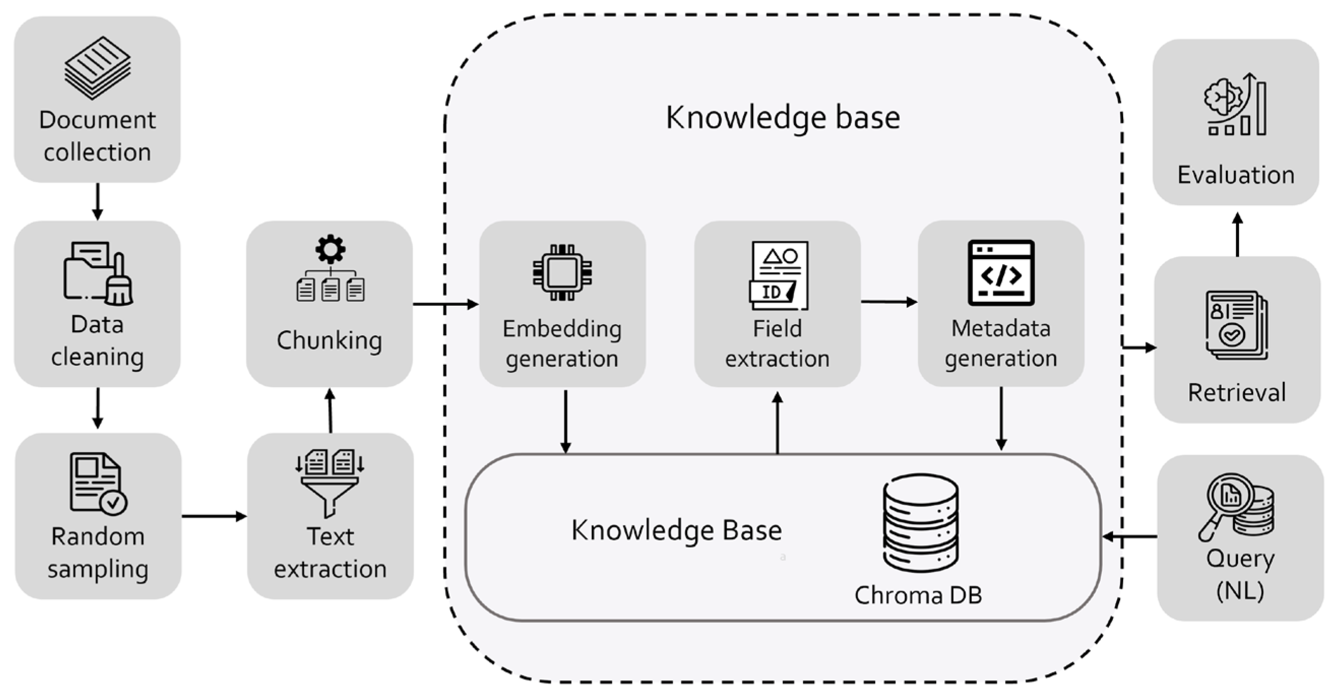
This section includes the methodology for constructing and evaluating a knowledge base for candidate information management, which consists of twelve main phases: (1) document collection, (2) data cleaning, (3) random sampling, (4) text extraction, (5) chunking, (6) embedding generation, (7) knowledge base construction using ChromaDB, (8) field extraction, (9) metadata extraction, (10) query, (11) retrieval, and (12) evaluation. Each phase incrementally contributes to the creation of a functional basic retrieval-based system suitable for human resource contexts.
As illustrated in Figure 1, the process is organized into sequential stages, beginning with document acquisition and concluding with system evaluation.

3.1. Document Collection

We begin with an institutional repository containing a large number of previously registered curricula vitae. This repository serves as the primary source for all subsequent processing steps. All documents are loaded into the system to establish the initial environment for extraction and knowledge base construction.

3.2. Data Cleaning

Before any extraction is performed, a cleaning stage is applied to reduce noise and prevent duplicated candidates from biasing the downstream evaluation. The initial corpus consisted of 5035 PDF CVs. In the cleaning procedure candidate records are grouped by an extracted candidate identifier and, for each group with repeated entries, a single representative document is retained while the remaining copies are removed from both the working directory and the associated intermediate collection in the vector database.
As a result of this curation step, 3707 PDF files were retained and stored as the cleaned corpus.

3.3. Random Sampling

From the full repository, a random subset of documents is selected to support experimental evaluation, and ensure computational feasibility (runtime constraints, CPU/RAM usage, and practical limitations of the computing environment). The methodological analysis was conducted on a representative subset of the curated corpus. Given a finite population of N = 3707 CVs, the target sample size was estimated using the finite population sampling formula in Equation (6), for an error equal to 5%:
n = 3707 · 1.96 2 · 0.5 ( 1 0.5 ) 0.05 2 3707 1 + 1.96 2 · 0.5 ( 1 0.5 ) = 348.17 350
Accordingly, an experimental target of 350 CVs was selected for primary evaluation profile (by rounding to the nearest integer).
For the remaining two evaluation profiles, a second random sampling step was applied, in this stage, the finite population corresponds to the experimental subset of N = 350 CVs, but the error incremented to 10%. Using the same conservative survey-sampling assumptions, the recommended sample size is:
n = 350 · 1.96 2 · 0.5 ( 1 0.5 ) 0.1 2 350 1 + 1.96 2 · 0.5 ( 1 0.5 ) = 75.53   76  
A reduced subsample of n = 76 CVs was adopted to decrease manual labeling workload and overall experimental cost while maintaining the same experimental design across scenarios. Under the same confidence and variability assumptions, using n = 76 implies a larger margin of error, it reduces annotation burden while still enabling consistent comparisons across scenarios.

3.4. Text Extraction

The selected documents go through an extraction process that converts each file into a structured textual representation. The text extraction was performed under a quality-gated sampling strategy targeting 350 valid CVs, meaning documents that not only yield usable textual content but also contain the minimum signal required for profile construction. In practice, only documents that meet extraction and content criteria; documents that fail are discarded and replaced until the target sample size is reached.
Depending on the format, Optical Character Recognition (OCR) or direct text parsing is applied. The extracted content is then cleaned and segmented into smaller units suitable for embedding. Relevant metadata, such as document type, sections, and identified entities, is also collected at this stage.

3.5. Chunking

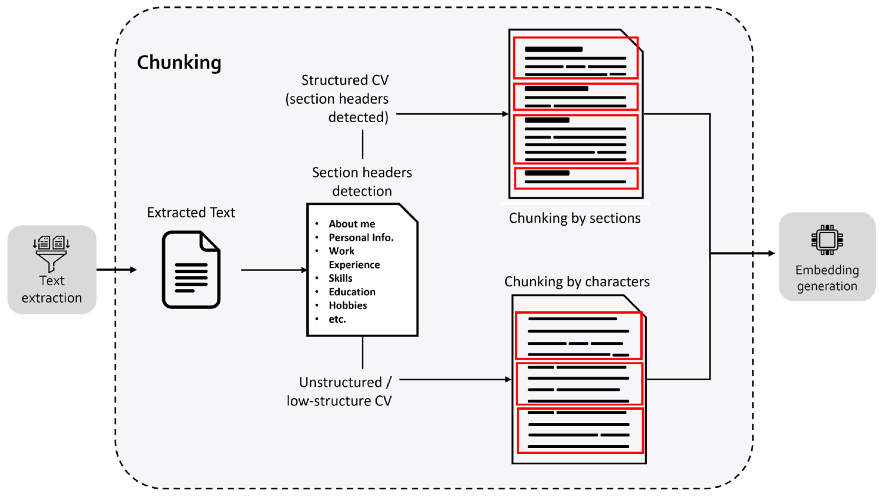
The extracted CV text is segmented into chunks to improve the granularity of se-mantic representations. Figure 2 provides an illustrated overview of this evaluation workflow.
Chunking is implemented with a two-stage strategy. First, the script attempts section-based chunking by detecting section headers in the extracted text. Section headers are detected using a combination of (i) a curated multilingual header list and (ii) typographic patterns such as uppercase lines and trailing colons. The text between consecutive headers is assigned to the corresponding section, and long sections are further split into fixed-length sub-chunks.
If fewer than two section headers are detected in a document, section-based chunking is considered unreliable and the script falls back to character-based chunking over the complete text. The fallback uses a maximum chunk length of 2000 characters with a 200-character overlap. Each produced chunk is stored with metadata describing its origin. At the document level, the indexing script stores the detected headers, the count of detected headers, the chunking method, and the total number of chunks.

3.6. Knowledge Base Construction

The knowledge base constitutes the core component of the methodology and is responsible for organizing, storing, and enabling access to the extracted information. This phase is composed of four tightly coupled sub-processes: embedding generation, field extraction, metadata generation, and vector storage.

3.6.1. Embedding Generation

Each chunk is transformed into a dense vector representation with the SentenceTransformers Python (3.10) Library (UKP Lab, Technical University of Darmstadt, Darmstadt, Germany), using the multilingual model paraphrase-multilingual-mpnet-base-v2 with no fine tuning applied. For each document, chunk embeddings are computed with the model encoder. These embeddings capture the semantic meaning of the content and provide the basis for similarity-based retrieval.
Embeddings and metadata are stored in a local ChromaDB persistent database. Two main collections are created: (i) for document-level records and (ii) for chunk-level records. The document identifier corresponds to the PDF filename.

3.6.2. Vector Storage in ChromaDB

The generated embeddings, associated metadata, and identifiers are stored in ChromaDB, which functions as the vector-based knowledge repository. ChromaDB indexes the embeddings and supports efficient similarity search while maintaining access to metadata for filtered retrieval.
Vector database management systems (VDBMSs) support similarity search through indexing methods designed for efficient approximate nearest neighbor retrieval, enabling scalable access to dense embeddings in real-world applications. These systems typically complement vector similarity with structured metadata to support filtered retrieval and more controlled selection behavior under task-specific constraints [31,32].
At this stage, the knowledge base is fully constructed and ready to support specialized field extraction.

3.6.3. Field Extraction

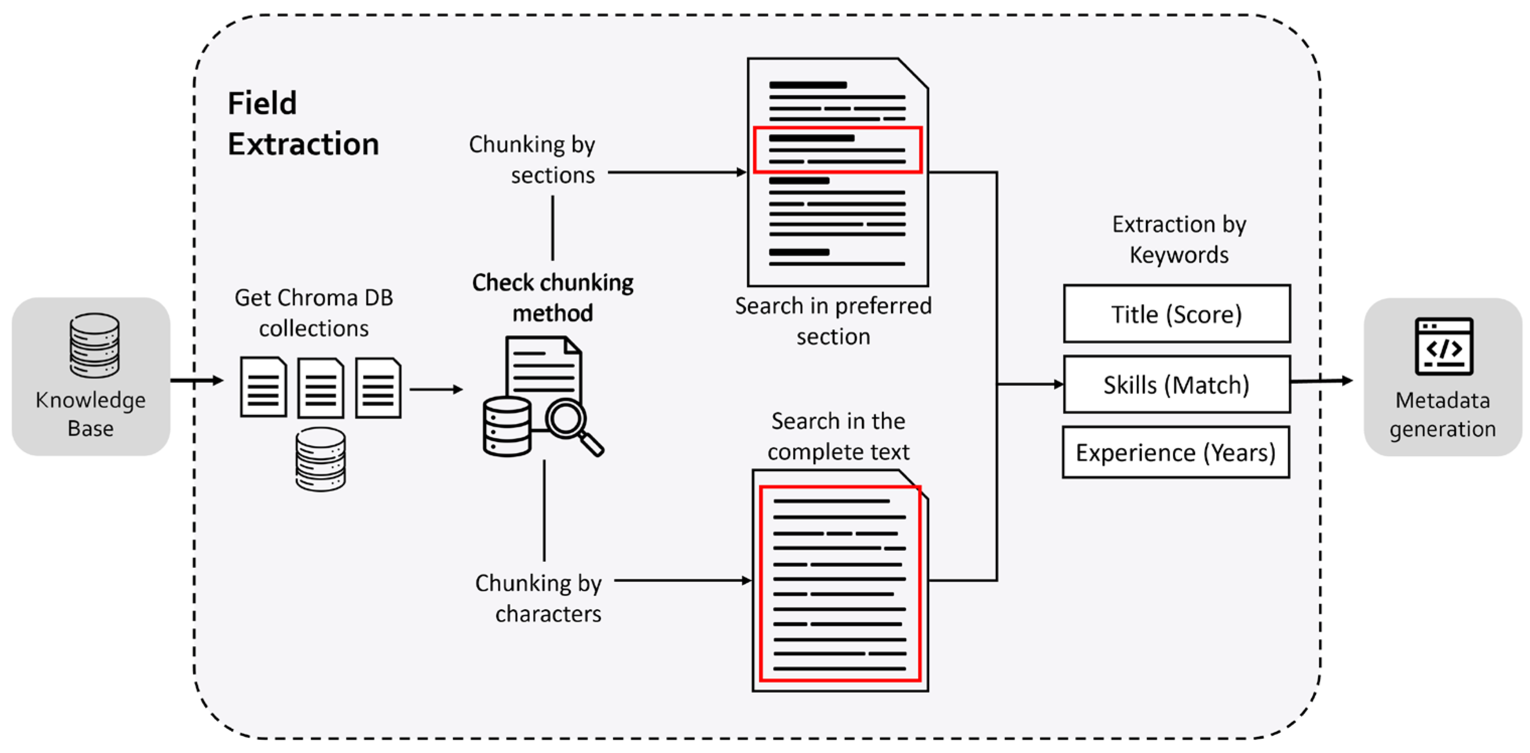
After indexing, enrichment of document metadata is done by extracting three high-value fields: job title, skills, and years of experience. A script reads document-level metadata, and retrieves the associated chunks using the filename metadata. Chunks are grouped by their section label to enable section-preferential extraction. Figure 3 provides an illustrated overview of this evaluation workflow.
Job title extraction searches the top chunk of the document and applies rule-based filtering and scoring. Candidate lines are filtered by removing contact-like strings, name repetitions, and section headers; remaining candidates are scored using role-hint terms, compactness (1–5 words), and top-of-document position. The best-scoring candidate above the acceptance threshold is stored as job title, together with a method label and the evidence line.
Skills extraction prioritizes chunks labeled as skills-related sections. When a skills header is detected, the subsequent lines are captured as a skills block and preserved for auditability. Keywords are then extracted by matching a curated skills dictionary using regular expressions. If no header is found, keyword matching is applied to the preferred text and then to the full document as a fallback. The output consists of a comma-separated keyword list and the number of unique matched skills.
Experience extraction estimates years of experience by applying regular expressions to either (i) chunks labeled as experience-related sections or (ii) the full document if no experience section is available or no match is found. The extractor supports year/month expressions (months converted to years) and date-range patterns as fallback evidence. The resulting integer and an evidence snippet are stored in the document metadata.

3.6.4. Metadata Generation

After field extraction, the extracted profile attributes are transformed into document-level metadata and persisted back into the knowledge base to enable structured filtering and future query operations.

3.7. Query (NL)

The system receives the user request, each request is treated as a query describing the type of candidate that should be retrieved. A query is written in natural language and contains three kinds of information: (i) what role or academic/professional profile is needed, (ii) which skills are required, and (iii) how many years of experience are expected. The system transforms the query into structured requirements and then checks whether each CV satisfies them using the metadata previously extracted from the documents.
Three natural language queries were used consistently to define candidate profiles in terms of professional degree/field of study, declared skills, and years of professional experience. These queries were kept fixed to ensure comparability of system behavior under different logical requirement combinations. Table 2 summarizes the query definitions.
For each experimental scenario, the retrieval task is formulated as a binary decision problem in which a curriculum either satisfies the specified set of requirements (positive class) or does not (negative class). Table 3 presents the evaluation scenarios used in the experimental setup. Each scenario represents a specific logical combination of three recruitment requirements, encoded as binary values, where “1” indicates that the requirement must be satisfied and “0” indicates that the requirement is not enforced. Scenarios 1 to 3 evaluate each requirement independently, Scenarios 4 to 6 assess pairwise combinations of requirements, and Scenario 7 represents the most restrictive case, in which all three requirements must be satisfied simultaneously.
For completeness, all three queries are executed under each of the seven evaluation scenarios. That is, for every scenario defined in Table 3, the retrieval script runs Query 1, Query 2, and Query 3 independently, producing three sets of candidate classifications per scenario. This gives that for each CV and each query, three binary indicators are computed: t for the degree/job-title requirement, s for the skills requirement, and e for the experience requirement. The experimental retrieval and evaluation operate on extracted, structured metadata (job title, skills, and years of experience) and apply a deterministic matching to derive a binary suitability decision for each scenario based on the logical combination of the required indicators. The title indicator t is set to 1 when the extracted job title is compatible with the target profile specified by the Query, and 0 otherwise. This compatibility is computed through a lightweight scoring procedure that rewards role-indicative patterns (e.g., role-ending tokens and compact title structure) and rejects non-title lines (e.g., contact-like strings or section headers). Box 2 summarizes the title-to-query matching procedure used in the evaluation.
Box 2. Title-to-query matching rule for computing the binary title applicability indicator.
Algorithm: Title-to-Query Matching
Inputs:
query_title     # e.g., “Mechanical Engineer”
detected_title    # e.g., “BE Mechanical” (from metadata extraction)
Resources:
t_dictionary[query_title] # list of synonyms/abbreviations/variants
role_hints = {“engineer”,”developer”,”analyst”,...} # role-ending tokens
degree_HINTS = {“be”,”b.e”,”b tech”,”btech”,...} # degree abbreviations
Output:
val_t {0,1}
Steps:
1) Normalize strings:
normalize(): lowercase, remove punctuation, collapse whitespace, remove accents
q = normalize(query_title)
t = normalize(detected_title)
2) Build list of acceptable title variants for the requested title:
variants = { q } all_title_variants(t_dictonary [q])
3) Direct match (highest priority):
if q == any variant in variants:
return val_t = 1
4) Fallback:
# Extract key “field token(s)” from query, e.g., “mechanical” from “mechanical engineer”
field_tokens = tokens(q)—role_hints
has_field  = t contains any word in field_words
has_role   = t contains any word in ROLE_WORDS
has_degree = t contains any word in DEGREE_WORDS
if has_field AND (has_role OR has_degree):
return val_t = 1
5) Otherwise:
return val_t = 0
The skills indicator s is set to 1 when the extracted skills list contains at least one of the query-required skills, and 0 otherwise. The experience indicator e is set to 1 when the extracted years of experience meet or exceed the query threshold and 0 otherwise.
These three indicators are then combined according to the active evaluation scenario. The resulting scenario-level decision constitutes the final retrieval output for the corresponding conditions.

3.8. Retrieval

For each query, the system then presents the retrieval results in a structured spreadsheet, together with the intermediate requirement indicators and the evidence fields used for traceability, evaluation and analysis.

3.9. Evaluation

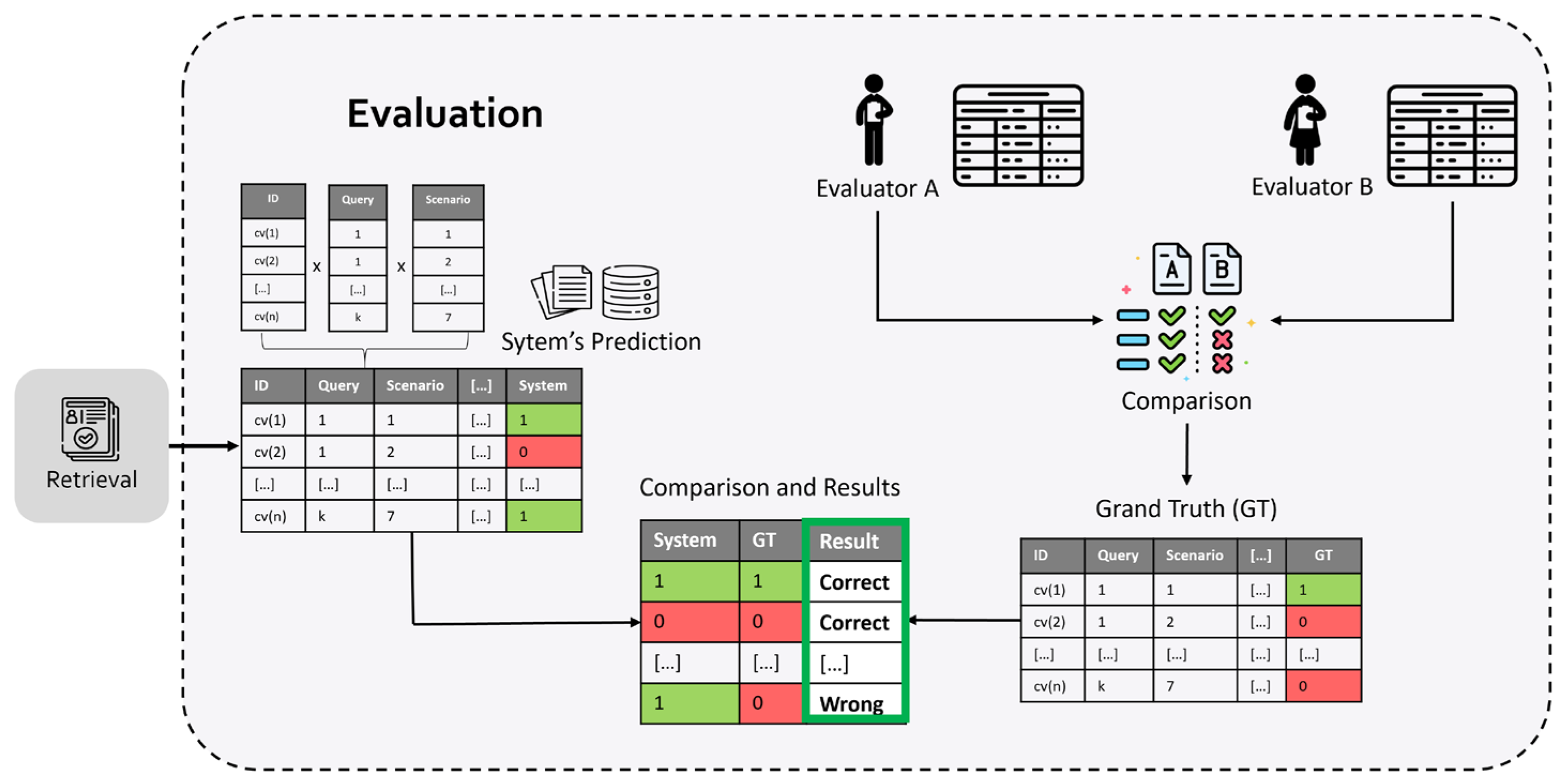
The evaluation is conducted by analyzing the ability of the candidate retrieval component to retrieve documents that satisfy the predefined logical combinations of recruitment requirements. The spreadsheet produced during retrieval is used as the central evaluation artifact.
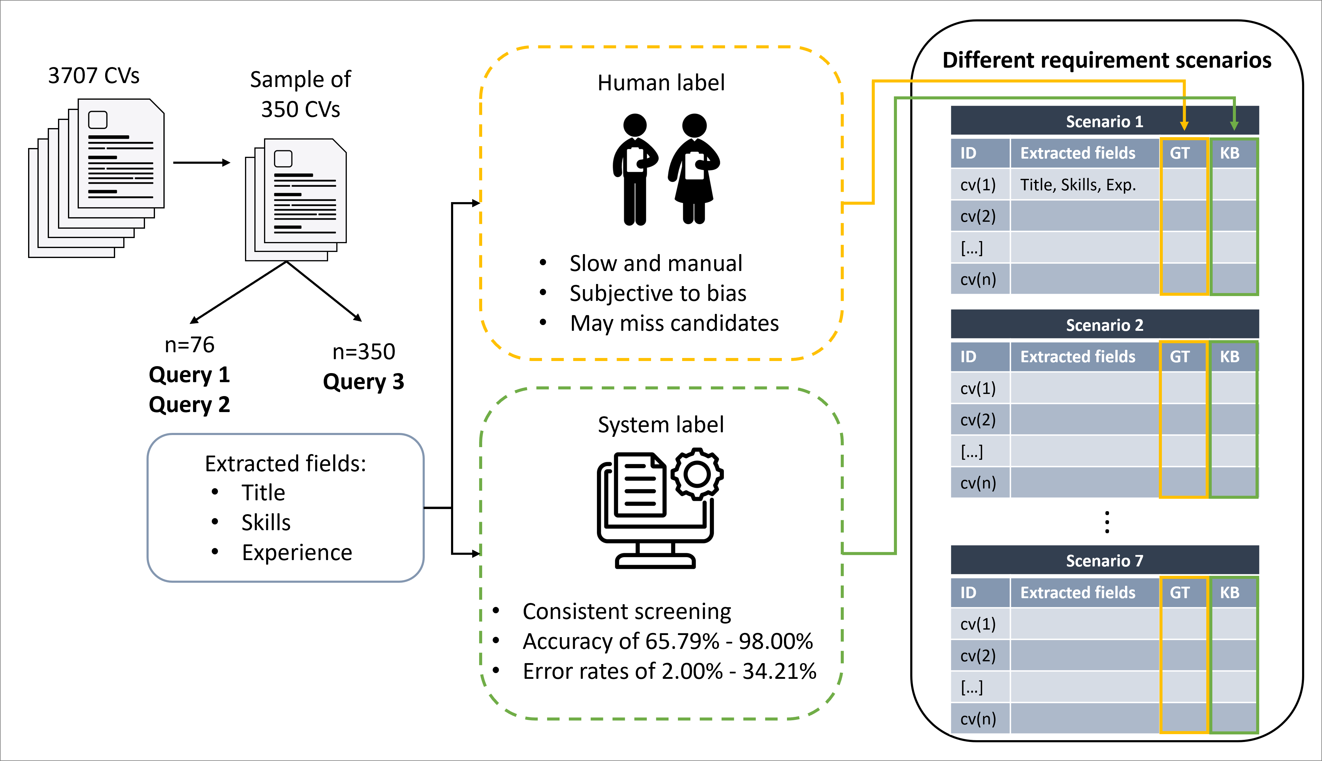
To obtain ground-truth labels, the same CV subset is independently reviewed and manually classified by two evaluators (Evaluator A and Evaluator B). Each evaluator assigns binary labels indicating whether a CV satisfies the requirements of the corresponding scenario. To assess the consistency of human labeling, inter-annotator agreement between Evaluator A and Evaluator B was quantified using Cohen’s kappa, which measures agreement beyond chance. This agreement analysis was performed for each query and scenario prior to ground-truth consolidation.
The two sets of human labels are then compared and reconciled to produce a consolidated ground-truth (GT) table, which is used as the final reference for analysis.
The automated classifications are then compared against the GT results, and a confusion matrix is constructed to quantify true positives, false positives, true negatives, and false negatives. Based on this matrix, different metrics are computed to measure the efficiency of the system. Figure 4 provides an illustrated overview of this evaluation workflow.
This evaluation is repeated across multiple scenarios with increasing constraint levels, allowing the analysis of system performance as the number of simultaneously required conditions increases.
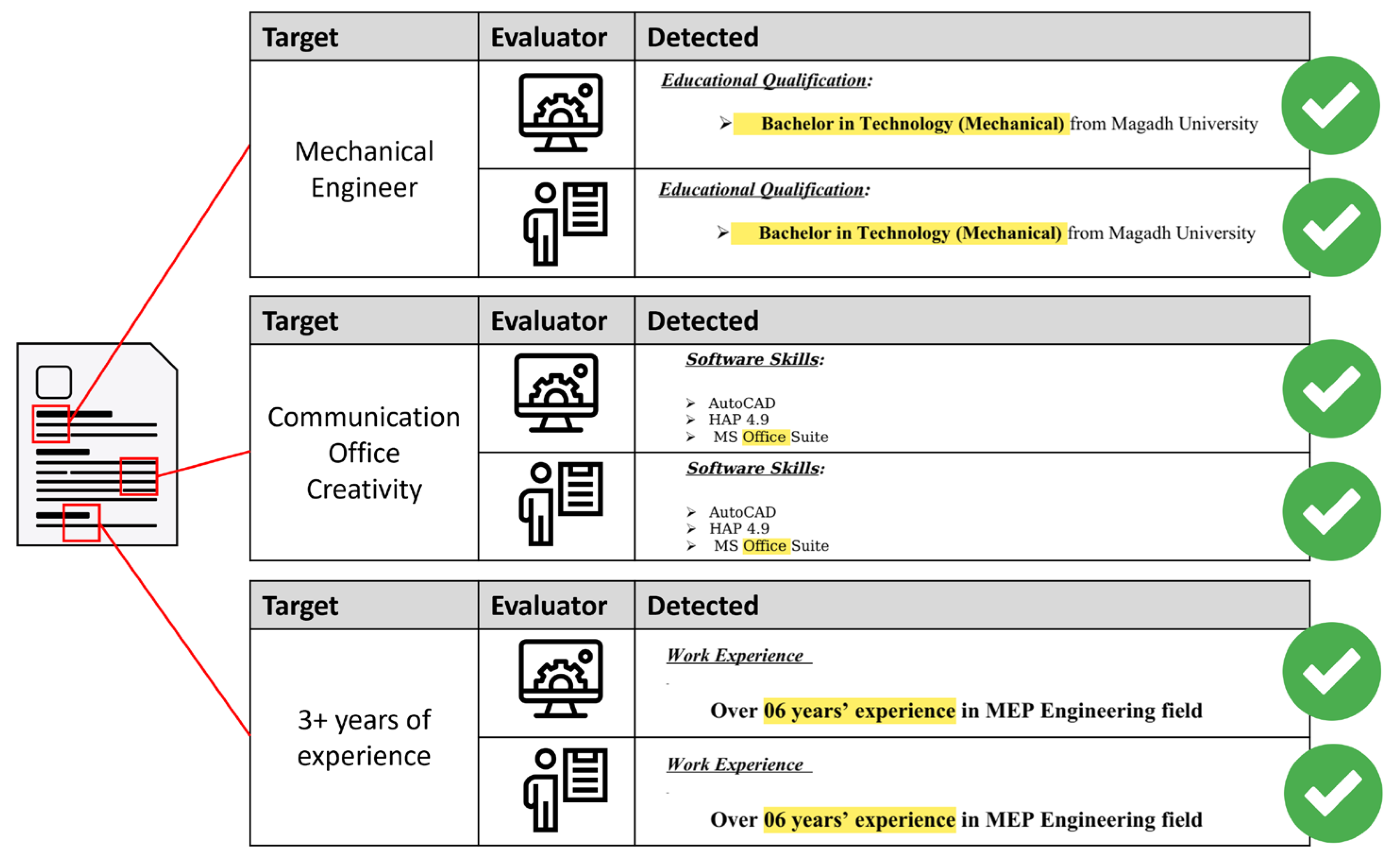
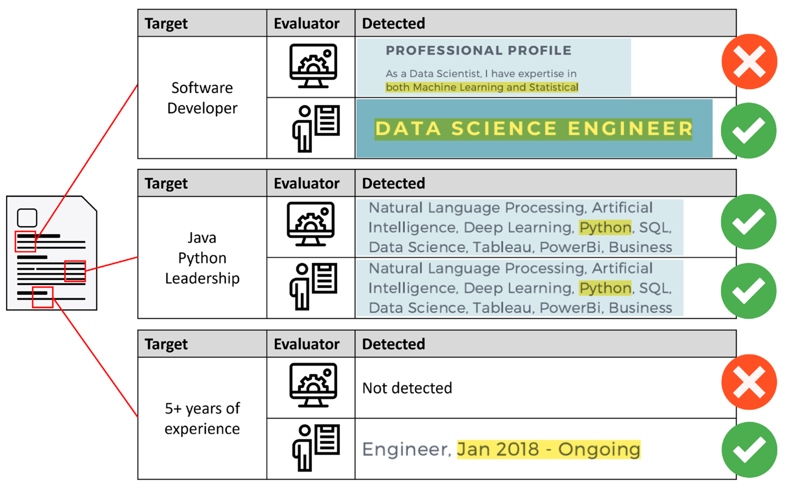
To complement the workflow shown in Figure 4, Figure 5 and Figure 6 provide qualitative illustrations of the requirement-matching step used during evaluation. These examples show how the three query dimensions (degree/title, skills, and experience) are compared against the fields detected in each CV, and how agreement or disagreement with human labels can occur depending on what evidence is successfully captured by the extraction and matching rules.
Figure 5 shows a representative case in which all three requirements are detected correctly, leading to agreement between the system decision and the human evaluator’s label. In this example, the detected title/degree evidence is compatible with the target profile, at least one of the required skills is matched in the detected skills list, and the extracted experience evidence satisfies the minimum years threshold.
Figure 6 shows a representative case with two incorrect detections, where the human evaluator confirms that the CV satisfies the query requirements based on visible evidence, but the automated pipeline fails to detect two of the required elements. This type of mismatch illustrates how false negatives may arise when relevant information is present in the document but is not captured by the extraction step or is missed by the matching criteria, particularly for title/degree and experience evidence expressed in formats that are difficult to normalize.

4. Results

This section reports the results obtained from the evaluation protocol defined in Section 3. Performance is reported across the seven evaluation scenarios and the fixed set of natural language queries, using accuracy, specificity, sensitivity, precision, error rate, and confusion-matrix outcomes against a human-labeled GT.
Before reporting system performance, inter-annotator agreement was examined to contextualize the reliability of the human-labeled reference used for GT construction. Agreement between Evaluator A and Evaluator B was quantified using Cohen’s kappa. The average kappa values were 0.58 for Query 1, 0.61 for Query 2, and 0.59 for Query 3, indicating a comparable level of labeling consistency across the three query profiles.
Given its substantially larger evaluation subset (n = 350), Query 3 is presented first, as it enables a more stable estimation of system behavior under varying constraint configurations and reduces sampling variability relative to Queries 1 and 2 (n = 76). The evaluation profile corresponding to Query 3 is defined as follows:

4.1. Results for Evaluation Profile: Query 3

Title: Mechanical Engineer
Skills: Communication, Office, Creativity
Experience: 3 years
Table 4 reports the confusion-matrix counts obtained for Query 3 under each of the seven evaluation scenarios.
From the confusion-matrix counts, Table 5 reports the derived performance metrics per scenario, including accuracy, specificity, sensitivity, precision, and error rate. This representation supports scenario-level comparison and highlights whether changes in agreement originate from false-positive inflation (over-selection) or false-negative inflation (missed eligible candidates).
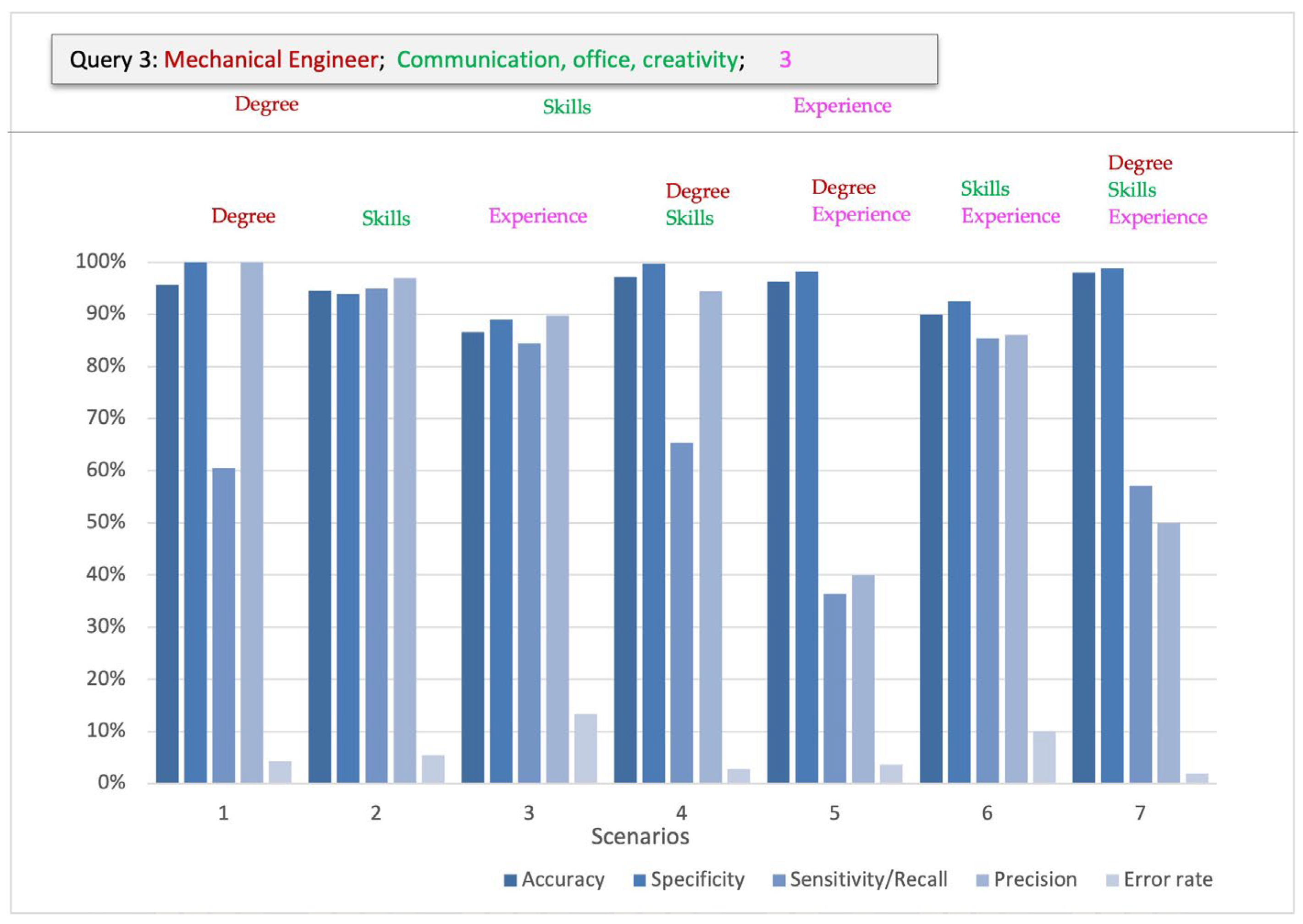
Figure 7 summarizes the same scenario-wise results for Query 3 by visualizing the five-evaluation metrics concurrently, facilitating comparison across single-requirement, dual-requirement, and fully integrated configurations.
Overall, Query 3 exhibits consistently high accuracy and specificity across scenarios, indicating robust rejection of non-eligible CVs. In contrast, sensitivity shows the largest scenario to scenario variation, confirming that positive detection is more sensitive to how much semantic evidence is jointly required. As constraints are integrated (two-attribute and three-attribute scenarios), error rate tends to decrease and the metric profile becomes more stable, suggesting that combining Degree, Skills, and Experience provides complementary evidence that reduces ambiguity in candidate eligibility decisions.
To determine whether similar performance patterns are observed under smaller evaluation subsets, the analysis now proceeds to Query 2 (n = 76).

4.2. Results for Evaluation Profile: Query 2

Title: Electrical Engineer
Skills: Leadership, Communication, AutoCAD
Experience: 4 years
Table 6 reports the confusion-matrix counts for Query 2 across the seven evaluation scenarios. These counts provide a transparent breakdown of correct classifications and error types under each logical requirement configuration.
Based on Table 6 and Table 7 presents the derived evaluation metrics for Query 2, reporting accuracy, specificity, sensitivity, precision, and error rate per scenario.
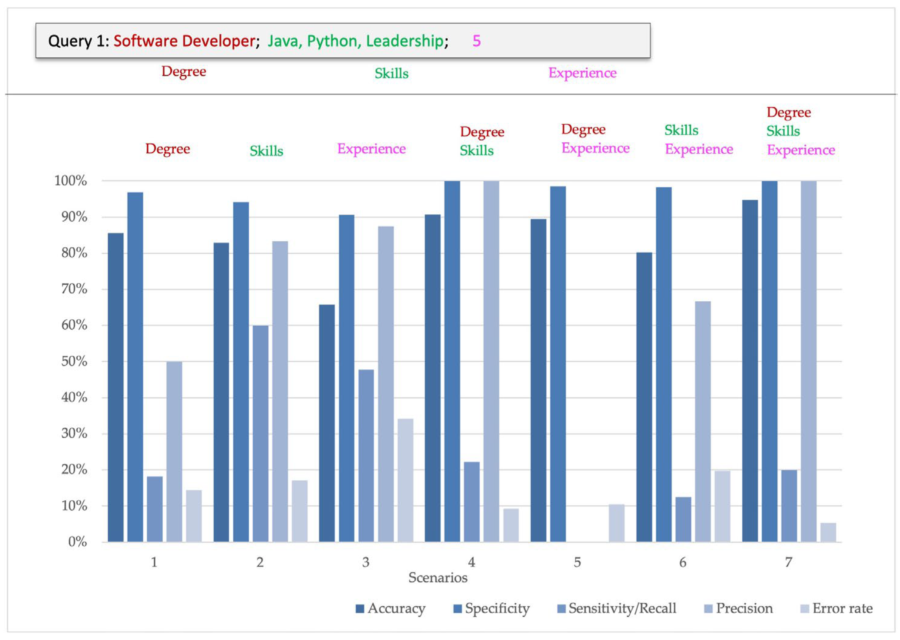
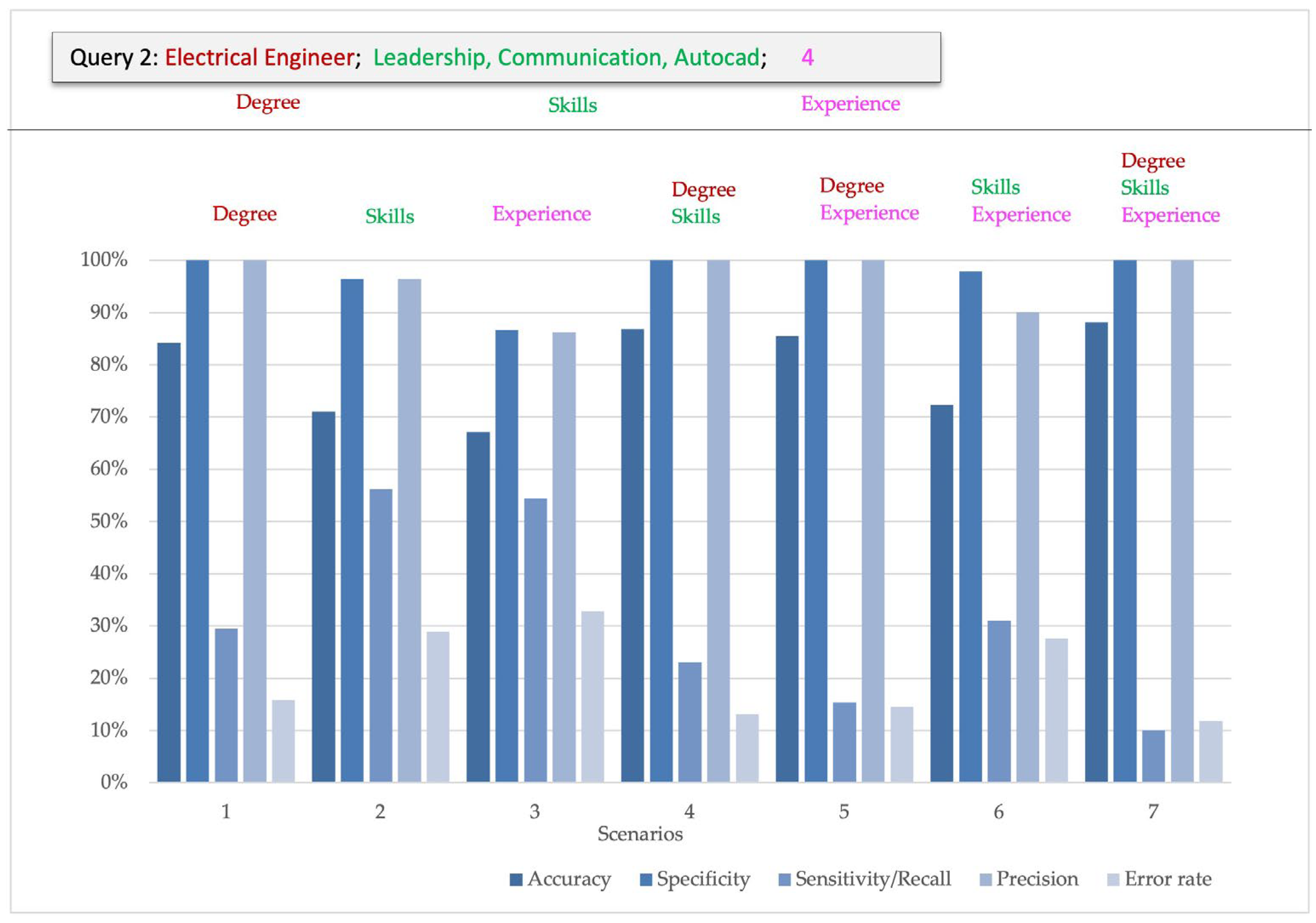
Figure 8 visualizes the performance metrics for Query 2 across scenarios, allowing rapid identification of configurations.
Query 2 shows high and stable specificity across scenarios, indicating that non-eligible CVs are rarely misclassified as suitable. However, sensitivity remains comparatively lower and more configuration-dependent, suggesting that identifying truly suitable candidates is more challenging than rejecting unsuitable ones. Dual-attribute and full-integration scenarios generally produce a more favorable balance between error rate and sensitivity, consistent with the interpretation that additional enforced evidence channels reduce borderline cases and improve discriminative behavior under requirement-driven screening.
To determine whether similar performance patterns are observed under equal evaluation subsets, the analysis now proceeds to Query 1 (n = 76).

4.3. Results for Evaluation Profile: Query 1

Title: Software Developer
Skills: Java, Python, Leadership
Experience: 5 years
For Query 1, Table 8 reports the confusion-matrix counts across the seven evaluation scenarios (n = 76). The table provides the basis for examining how the error profile changes as the system transitions from single-requirement screening to multi-requirement enforcement in Query 1.
Table 9 reports the performance metrics derived from Table 8, including accuracy, specificity, sensitivity, precision, and error rate for each scenario.
Figure 9 summarizes the scenario-wise metric profile for Query 1 and highlights how requirement integration modulates the trade-off between rejecting non-eligible candidates and successfully confirming eligible ones.
Query 1 maintains high specificity across scenarios, indicating that false positives remain limited under most configurations. Nevertheless, sensitivity shows notable fluctuation and tends to remain lower than specificity, reflecting that missed eligible candidates (false negatives) are a more prominent failure mode than over-selection.
Performance generally improves when multiple requirements are enforced simultaneously, supporting the notion that semantic complementarity among Degree, Skills, and Experience helps stabilize decisions. However, the persistence of sensitivity variability indicates that positive evidence is sensitive to how candidate information is expressed and captured by the upstream extraction rules, particularly for title and experience representations.

4.4. Derived Performance Metrics Across Scenarios

To provide a scenario-level synthesis of classification performance, we computed derived agreement metrics across all evaluation queries. Table 10 presents the agreement rate (accuracy, expressed as a percentage) between the automated classifications and the GT labels for each query under the seven evaluation scenarios.
To facilitate cross-scenario comparison, we calculated an average value for each scenario as the arithmetic mean of the three query-level accuracy results. This aggregated measure summarizes overall performance per scenario under a fixed set of query definitions and provides a compact indicator of how agreement varies as the constraint configuration changes across scenarios.
The scenario-level averages indicate that Scenario 7 achieves the highest overall agreement in the evaluated sample, while Scenario 3 shows the lowest average agreement across the three queries. Intermediate values are observed for the remaining scenarios, suggesting that agreement levels vary with the logical combination of enforced requirements.
To complement the agreement-based summary, Table 11 reports sensitivity between the automated classifications and the GT labels for each evaluation query across the seven scenarios. To facilitate scenario-level comparison, an average value is computed for each scenario as the arithmetic mean of the three query-level sensitivity results. This summary highlights how effectively the system identifies eligible candidates as constraint configurations vary, and it is particularly informative in settings where accuracy may remain high due to a predominance of true negatives.
The scenario-level averages in Table 11 indicate that Scenario 2 yields the highest mean sensitivity across the three queries, while Scenario 5 shows the lowest average sensitivity. Intermediate values are observed for the remaining scenarios, confirming that sensitivity is strongly influenced by the enforced requirement combination and varies more substantially than agreement-based metrics.
To summarize the system’s ability to avoid false-positive selections under varying constraint strictness, Table 12 reports specificity per query across the seven scenarios, with an Average computed as the arithmetic mean across queries.
A clear pattern in Table 12 is the consistently high specificity across all configurations. The scenario-level averages show that Scenario 4 achieves the highest mean specificity, while Scenario 3 exhibits the lowest average specificity. The remaining scenarios remain close to the upper bound, indicating stable rejection of non-eligible candidates across query profiles.

4.5. Worst-Case vs. Best-Case Scenario Comparison: Query 3

To illustrate how performance indicators are derived and to provide a transparent view of classification behavior, we present confusion matrices for Query 3 under two representative constraint configurations: the scenario with the lowest accuracy (Scenario 3) and the scenario with the highest accuracy (Scenario 7). These two cases were selected because they represent contrasting evaluation results between a lower-agreement configuration and a high-agreement configuration, enabling a more interpretable comparison of error profiles as constraint strictness increases.
Table 13 depicts the confusion matrix for Query 3 under Scenario 3. Table 14 reports the corresponding contingency table, which forms the basis for computing accuracy, specificity, sensitivity, precision and error rate.
In this scenario, both false positives and false negatives are observed, indicating that relying on the Experience-only constraint can yield mixed evidence and a less stable eligibility boundary. While sensitivity remains relatively high, the error reflects those incorrect acceptances and missed suitable candidates coexist in this configuration.
Table 15 presents the confusion matrix for Query 3 under Scenario 7, where the system achieved the highest accuracy (%). Table 16 reports the corresponding contingency table.
In Scenario 7, the matrix indicates a strong rejection tendency driven by a very large number of true negatives, which explains the high accuracy and specificity. However, positive-class confirmation remains challenging: the system retrieves 4 true positives but also produces 4 false positives, yielding a Precision of 50.00%, while 3 false negatives reduce sensitivity to 57.14%.

4.6. Worst-Case vs. Best-Case Scenario Comparison: Query 2

To provide an interpretable, scenario-level view of classification behavior for Query 2, we report confusion matrices under two representative constraint configurations: the lowest accuracy scenario (Scenario 3) and the highest accuracy scenario (Scenario 7).
Table 17 reports the confusion-matrix counts for Scenario 3 and Table 18 the derived metrics.
Query 2 in scenario 3 shows the lowest agreement, with a substantial number of false negatives and false positives. This yields moderate sensitivity despite relatively high precision, suggesting that the Experience-only configuration tends to miss a relevant portion of eligible candidates while still introducing some over-inclusion.
Table 19 reports the confusion-matrix counts for Scenario 3 and Table 20 the derived metrics.
In Scenario 7, Query 2 achieves its highest agreement with perfect specificity and precision, reflecting zero false positives. Nevertheless, sensitivity remains low due to a high number of false negatives, indicating a strongly conservative acceptance behavior under the all-requirements constraint. In this setting, agreement is largely driven by correct rejections.

4.7. Worst-Case vs. Best-Case Scenario Comparison: Query 1

For Query 1, we also report two representative configurations to illustrate contrasting error profiles: the lowest accuracy scenario (Scenario 3) and the highest accuracy scenario (Scenario 7). Table 21 reports the confusion-matrix for Scenario 3 and Table 22 the derived metrics, while Table 23 and Table 24 report the corresponding results for Scenario 7.
In Scenario 3, Query 1 obtains low accuracy, driven primarily by a large number of false negatives and a smaller but present set of false positives. This produces a comparatively low sensitivity while maintaining high precision.
This Scenario achieves a high agreement with perfect specificity and precision, reflecting zero false positives. However, sensitivity remains limited due to false negatives, meaning that most eligible candidates are not confirmed under the strict all-requirements condition.
Across the three query profiles, a consistent pattern is observed: Scenario 3 yields the lowest agreement, whereas Scenario 7 yields the highest agreement. This contrast suggests that single-attribute enforcement (Experience-only) provides an insufficiently stable eligibility boundary, leading to increased misclassifications, while full semantic integration (Degree + Skills + Experience) strengthens discrimination by requiring convergent evidence across attributes. However, the strictness of Scenario 7 can also increase conservative behavior by favoring correct rejections over positive confirmations, which may reduce sensitivity in some cases.
Overall, the reported results summarize system performance across scenarios and queries, and the case study for each query provides a more detailed view through confusion-matrix outcomes and derived metrics.
We evaluated three queries under a repeated measures design, including seven related scenarios (Scenario 1–Scenario 7). Given that the dependent variables were dichotomous (Correct = 1; Failure = 0), non-parametric tests were applied. Global differences were examined using the Friedman test and Cochran’s Q test, followed by Wilcoxon signed-rank post hoc comparisons.

4.8. Statistical Test for Query 1

Query 1 contains 76 CVUs; before applying the statistical test, the results are: Friedman test: χ2(6) = 42.27, p < 0.001; Cochran’s Q: Q(6) = 42.271, p < 0.001. These results indicate statistically significant differences among scenarios; Table 25 and Table 26 show the details for the Friedman test; meanwhile, * D = Degree; S = Skills; E = Experience.
Table 27 and Table 28 have the details for Cochran’s Q test; and Table 29 shows the comparisons among scenarios using the Wilcoxon test.
As the previous results show that Scenario 7 is the best-performing scenario, we conducted pairwise comparisons using Wilcoxon signed-rank tests, contrasting each scenario against Scenario 7 (see Table 29).
The statistical analysis revealed significant differences among the seven scenarios (Friedman χ2(6) = 42.27, p < 0.001; Cochran’s Q(6) = 42.271, p < 0.001). The ranking structure identified Scenario 7 as the highest-performing condition, while Scenario 3 exhibited the lowest performance.
Wilcoxon pairwise comparisons confirmed that Scenario 7 significantly outperformed most alternative scenarios, particularly Scenario 3, which showed the largest deviation. Scenario 4 demonstrated performance closest to Scenario 7, with no statistically significant difference observed between them.
These findings indicate a clear performance hierarchy, with Scenario 7 representing the optimal configuration under Query 1 conditions.

4.9. Statistical Test for Query 2

The statistical analysis for Query 2, conducted with a sample size of 76 CVUs, revealed significant differences among the seven scenarios. The Friedman test yielded χ2(6) = 28.95, p < 0.001, while Cochran’s Q test produced Q(6) = 28.948, p < 0.001, confirming the presence of statistically significant variability across conditions. Table 30 and Table 31 present the detailed results of the Friedman test, including mean rank distributions, whereas * D = Degree; S = Skills; E = Experience
Table 32 and Table 33 summarize the outcomes of Cochran’s Q test. Furthermore, Table 34 reports the pairwise Wilcoxon signed-rank comparisons, which provide additional insight into the specific differences between scenarios.
As in Query 1, Scenario 7 showed the best performance; hence, we conducted pairwise comparisons using Wilcoxon signed-rank tests, contrasting each scenario against Scenario 7 (see Table 34).
For Query 2, both Friedman and Cochran’s Q tests again identified statistically significant differences among scenarios (χ2(6) = 28.95, p < 0.001; Q(6) = 28.948, p < 0.001).
Although Scenario 7 maintained the highest mean rank, the magnitude of differences among scenarios was smaller compared to Query 1. Wilcoxon test analyses showed that Scenario 7 significantly outperformed Scenario 2, Scenario 3, and Scenario 6. Yet that same test showed no significant difference among Scenario 7 and Scenario 1, Scenario 4, and Scenario 5. This suggests that, under Query 2 conditions, the superiority of Scenario 7 becomes less pronounced, and Scenario 4 again emerges as a statistically comparable alternative. Scenario 3 consistently remains the weakest-performing configuration.

4.10. Statistical Test for Query 3

The results for Query 3, based on a larger sample size (n = 350), revealed highly significant differences among the seven scenarios. The Friedman test produced χ2(6) = 83.28, p < 0.001, while Cochran’s Q test yielded Q(6) = 83.282, p < 0.001, confirming the existence of statistically significant variability across conditions. The ranking structure observed in previous queries was replicated under increased statistical power, reinforcing the stability and robustness of the performance hierarchy. Table 35 and Table 36 present the detailed outcomes of the Friedman test, whereas * D = Degree; S = Skills; E = Experience.
Table 37 and Table 38 summarize the results of Cochran’s Q test. Additionally, Table 39 reports the Wilcoxon signed rank pairwise comparisons, providing further insight into the specific differences between scenarios.
Finally, as in the previous two queries, Scenario 7 outperformed the other scenarios; hence, we carried out pairwise comparisons using Wilcoxon signed-rank tests, contrasting each scenario against Scenario 7 (see Table 39).
Query 3, based on a substantially larger sample (n = 350), produced highly significant global differences (Friedman χ2(6) = 83.28, p < 0.001; Cochran’s Q(6) = 83.282, p < 0.001).
For Query 3, which was evaluated using a larger sample size (n = 350), the analysis revealed highly significant global differences across the seven scenarios. The Friedman test yielded χ2(6) = 83.28 (p < 0.001), and Cochran’s Q test produced Q(6) = 83.282 (p < 0.001). The larger sample size reinforced the ranking structure previously observed in Queries 1 and 2. Scenario 7 continued to exhibit the highest performance, whereas Scenario 3 consistently demonstrated the lowest ranking
Wilcoxon comparisons indicated that Scenario 7 significantly outperformed Scenarios 1, 2, 3, 5, and 6, with the strongest difference observed against Scenario 3. As in previous queries, the test did not find a statistical difference between Scenario 7 and Scenario 4. Replicating this ranking structure across a larger sample reinforces the robustness and internal consistency of the experimental results.
Finally, the results consistently demonstrate statistically significant differences among the seven scenarios across all three queries (p < 0.001). Scenario 7 achieved the highest performance in every case, whereas Scenario 3 consistently exhibited the lowest performance. The larger sample size in Query 3 reinforced the statistical evidence and confirmed the stability of the ranking structure previously observed in Queries 1 and 2 (see Table 40).
The comparative analysis across the three queries suggests that the structural components of each scenario play a decisive role in determining performance outcomes. In particular, the configuration and alignment of Degree and Skills emerge as the primary factors influencing correctness rates across scenarios. Scenarios that demonstrate higher levels of coherence between academic background (Degree) and declared competencies (Skills) consistently achieve superior rankings, as observed in the sustained dominance of Scenario 7. Conversely, scenarios in which the Degree or Skills does not appear either one or tend to exhibit lower performance, as reflected in the persistent underperformance of Scenario 3.
These findings indicate that the interaction between formal academic qualifications and explicitly defined skills constitutes a critical determinant of scenario effectiveness. The stability of this pattern across different sample sizes further reinforces the structural relevance of these elements in shaping performance outcomes. Table 41 presents a summary of the p-values across the three queries, comparing each scenario against Scenario 7 using the Wilcoxon signed-rank test.
Together, these findings quantify the system’s agreement with human labeling under different constraint configurations and motivate the interpretation presented in Section 5.

5. Discussion

The reported results indicate that system performance depends on the logical structure of the enforced recruitment requirements and by how much semantic evidence is jointly required to declare a curriculum as suitable. Across the three evaluation profiles, the Scenario-wise metric summaries (Figure 7, one per query) show a consistent pattern: specificity remains high under most configurations, while sensitivity exhibits the largest fluctuations, particularly when a single requirement is enforced.
A common trend across queries is a monotonic improvement with dimensional integration. Under the strictest configuration (Scenario 7: Degree + Skills + Experience), the system generally reaches its highest accuracy and near-ceiling specificity, while the error rate becomes minimal. These outcomes suggest that semantic complementarity among the three attributes is practically important: enforcing multiple conditions simultaneously reduces spurious acceptances and stabilizes decision behavior.
Confusion-matrix-derived metrics provide a more diagnostic view of system behavior [21,33]. Together, these outcomes indicate that enforcing stricter requirement combinations can strengthen the rejection of non-eligible candidates (reflected in consistently high specificity and large true-negative counts), but may also reduce the system’s ability to confirm truly suitable candidates when positive evidence is missing, ambiguously phrased, dispersed across sections, or not fully captured by the upstream field-extraction and metadata representation stages. Several limitations should be considered. First, Queries 1 and 2 rely on a smaller subset (n = 76) compared to Query 3 (n = 350), so cross-query differences may partially reflect differences in representativeness and metric variance rather than purely methodological effects. Second, the experimental design uses a fixed set of three query profiles, which limits conclusions about broader occupational categories and skill distributions. Third, a limitation that should also be considered is the possibility of domain-related annotation bias. The GT labels were produced by evaluators with an academic background in computer systems, which may have influenced how certain profiles were interpreted and judged. In particular, Query 1 (Software Developer) may have been evaluated with greater implicit expertise and stricter expectations regarding what constitutes sufficient evidence for degree/title alignment, skill relevance, or experience adequacy. Even when labeling guidelines are consistent, such background knowledge can affect borderline decisions and thereby influence confusion-matrix outcomes. Finally, computational constraints influenced experimental scale and may restrict the extent to which performance can be extrapolated to larger deployments.
An additional factor influencing retrieval effectiveness is the formulation of the user query, which can be interpreted as a prompt-design problem. Because the system operationalizes the query as structured constraints (degree/title, skills, and experience), more specific or narrowly phrased requirements can reduce retrievability, while broader query formulations may increase coverage but can expand the eligibility boundary under single-requirement settings. This highlights that retrieval performance is driven not only by system design, but also by query engineering, which modulates how likely requested attributes are detected and validated against metadata.
Lexical variability in query formulation can also affect match reliability, particularly for the degree/job-title constraint. Titles are frequently expressed using abbreviations, synonyms, or seniority variants, such that a semantically correct match may be missed when the requested role is phrased differently from the document. Moreover, CVs do not always report a job title explicitly, and when a title is present it may fall outside the current detection window and therefore not be captured by the system. In the implemented scripts, this effect is partially mitigated through curated term dictionaries and role-hint keywords used during title detection, but increasing query specificity can amplify mismatch risk when relevant variants are not covered. For years of experience, applicants use heterogeneous formats (explicit numeric statements, date ranges, and open-ended expressions such as “ongoing” or “present”). When the phrasing falls outside the temporal patterns recognized by the extraction rules, experience values may be underestimated or not detected, propagating into false negatives under experience-enforced scenarios. By comparison, skills matching is less impacted because it is primarily presence-based; however, skill terms may appear outside a competency context, and the current implementation does not enforce contextual validation, which can introduce noise in borderline cases.
The statistical analysis made provides formal support for the scenario-level performance hierarchy observed in the metric tables. Because outcomes were binary, non-parametric repeated-measures tests were applied; the Friedman test and Cochran’s Q test confirmed statistically significant differences among scenarios for all queries (p < 0.001). The ranking structure was consistent, with Scenario 7 (Degree + Skills + Experience) achieving the highest performance and Scenario 3 the lowest, indicating that performance is systematically linked to how evidence is combined in the enforced requirement structure.
Post hoc Wilcoxon comparisons further indicate that the advantage of Scenario 7 is not uniform across all alternatives. In particular, Scenario 4 was consistently the closest condition to Scenario 7 and did not exhibit statistically significant differences against Scenario 7 in the three queries.
Future research may extend this work in two directions. First, controlled comparisons could be conducted to isolate the contribution of the proposed knowledge base design methodology by contrasting it with less structured implementations while keeping the dataset, queries, and evaluation protocol fixed. Such analyses would help determine whether methodological components such as metadata design, identifier construction, and storage organization measurably influence retrieval and classification outcomes. Second, it would be valuable to study the impact of incorporating a Large Language Model (LLM) into the retrieval pipeline, for example through LLM-assisted reranking or structured validation of extracted attributes (Degree, Skills, and Experience). Evaluating these variants under the same seven-scenario framework could clarify whether LLM integration reduces false positives in flexible configurations and improves precision under strict multi-requirement scenarios.

6. Conclusions

This work presented a structured methodology for constructing and evaluating a knowledge-base-driven pipeline for candidate information management in recruitment settings. The approach organizes the workflow from document ingestion and information extraction to embedding-based storage in a vector repository and requirement-driven retrieval, enabling systematic querying and analysis of candidate profiles using predefined selection criteria. The proposed design further emphasizes traceability by preserving evidence snippets and method labels during field enrichment, supporting auditability of retrieval decisions.
The experimental evaluation demonstrated that performance varies across constraint configurations and query profiles. Across all three queries, specificity remained consistently high and stable, indicating robust negative classification and a low tendency to over-select non-eligible candidates. In contrast, sensitivity showed the greatest dispersion across scenarios, highlighting that the ability to recover suitable candidates is strongly configuration-dependent and improves when Degree, Skills, and Experience are jointly enforced. While agreement-based results provide a global summary, the confusion-matrix analysis for representative scenarios showed that accuracy alone may not capture the underlying error profile. In particular, confusion-matrix-derived metrics such as specificity, sensitivity, precision and error rate are necessary to interpret whether the system tends to over-select candidates (false positives) or miss eligible profiles (false negatives) under different requirement combinations.
Although the experimental scale was constrained by time and computational resources, the reported results establish a transparent baseline and an evaluation framework that can be reused to assess future variants of retrieval-based candidate selection systems. The analysis also indicates a sample-size effect: the larger evaluation subset (Query 3) exhibited reduced metric dispersion and greater statistical stability, suggesting that representativeness influences both robustness and interpretability of the reported outcomes.
The experimental results and statistical testing demonstrate that scenario structure is a decisive factor in system behavior. Across all three evaluated queries, global tests confirmed significant differences among the seven scenarios, and a stable ranking structure emerged across sample sizes. These findings reinforce the conclusion that semantic evidence is complementary and that performance improves as constraints integrate multiple sources of candidate information rather than relying on a single attribute. At the same time, post hoc comparisons highlight that maximal strictness is not the only effective configuration. This result is practically relevant for recruitment settings where experience expressions are highly heterogeneous and may be harder to normalize reliably.
Overall, the study supports the use of structured knowledge base design and scenario-based evaluation as a practical foundation for improving consistency and interpretability in recruitment workflows. Future extensions may improve sensitivity under sparse-evidence cases by refining query formulation strategies and expanding domain dictionaries for title/skill variants, while maintaining the high specificity observed across configurations.

Author Contributions

Conceptualization, S.M.-Z. and M.P.P.-F.; methodology, S.M.-Z.; validation, S.M.-Z., M.P.P.-F., G.C.-V., J.F.-S., J.J.G.-B. and E.A.-R.; formal analysis, S.M.-Z.; investigation, S.M.-Z.; resources, S.M.-Z.; data curation, S.M.-Z.; writing—original draft preparation, S.M.-Z.; writing—review and editing, S.M.-Z., M.P.P.-F., G.C.-V., J.F.-S., J.J.G.-B. and E.A.-R.; visualization, S.M.-Z.; supervision, M.P.P.-F.; project administration, M.P.P.-F. All authors have read and agreed to the published version of the manuscript.

Funding

This research received no external funding.

Institutional Review Board Statement

Not applicable.

Informed Consent Statement

Not applicable.

Data Availability Statement

The dataset used in this study is publicly available through Kaggle (NER Annotated CVs) and Hugging Face (Annotated NER PDF Resumes). The code used for data ingestion, retrieval, and evaluation is available in the public GitHub (Github3.19.0, Inc., San Francisco, CA, USA) repository: https://github.com/sofi1813/hr-knowledge-base-retrieval-system (accessed on 1 March 2026).

Acknowledgments

The authors would like to thank Emmanuel Aran-Hernandez for technical support, including the development of the experimental codebase, execution of the computational experiments, and provision of the resulting outputs used in this study. During the preparation of this manuscript/study, ChatGPT (OpenAI, San Francisco, CA, USA; model: GPT-5) was used to assist in structuring and refining the manuscript language. The authors reviewed and edited all AI-generated outputs and take full responsibility for the content of this publication.

Conflicts of Interest

The authors declare no conflicts of interest.

Abbreviations

The following abbreviations are used in this manuscript:
LLMLarge Language Model
NLPNatural Language Processing
CVCurriculum Vitae
OCROptical Character Recognition
GTGrand Truth
TPTrue Positive
TNTrue Negative
FPFalse Positive
FNFalse Negative

References

  1. Yang, B.; Shen, Z. Knowledge graph construction and talent competency prediction for human resource management. Alex. Eng. J. 2025, 121, 223–235. [Google Scholar] [CrossRef] [Scilit]
  2. Mutukwa, M.K.; Mupeta, M. Design and Development of an Online Recruitment Systems for Small And Medium-Sized Enterprises In Zambia. Certif. J. Int. J. Adv. Eng. Manag. (IJAEM) 2025, 7, 1063–1077. [Google Scholar] [CrossRef] [Scilit]
  3. Giabelli, A.; Malandri, L.; Mercorio, F.; Mezzanzanica, M.; Seveso, A. Skills2Job: A recommender system that encodes job offer embeddings on graph databases. Appl. Soft Comput. 2021, 101, 107049. [Google Scholar] [CrossRef] [Scilit]
  4. Ngonadi, I.V.; Joshua, C.O.; Ighosotu, J.O. Simulating an Automated Staff Recruitment Management System. Int. J. Adv. Eng. Manag. (IJAEM) 2021, 3, 1892. [Google Scholar] [CrossRef]
  5. NER Annotated CVs. Available online: https://www.kaggle.com/datasets/mehyarmlaweh/ner-annotated-cvs (accessed on 15 December 2025).
  6. Mehyaar/Annotated_NER_PDF_Resumes · Datasets at Hugging Face. Available online: https://huggingface.co/datasets/Mehyaar/Annotated_NER_PDF_Resumes (accessed on 16 December 2025).
  7. Herdiyanto, R.F.; Maylawati, D.S.; Lukman, N. Automatic abstractive summarization of Curriculum Vitae using S-Bert and T5. JIKO (J. Inform. Dan Komput.) 2025, 8, 103–112. [Google Scholar] [CrossRef] [Scilit]
  8. Sathyanarayanan, S. Confusion Matrix-Based Performance Evaluation Metrics. Afr. J. Biomed. Res. 2024, 27, 4023–4031. [Google Scholar] [CrossRef] [Scilit]
  9. Zeng, G. Invariance Properties and Evaluation Metrics Derived from the Confusion Matrix in Multiclass Classification. Mathematics 2025, 13, 2609. [Google Scholar] [CrossRef] [Scilit]
  10. Yang, S.; Berdine, G. Confusion matrix. Southwest Respir. Crit. Care Chron. 2024, 12, 75–79. [Google Scholar] [CrossRef] [Scilit]
  11. Rainio, O.; Teuho, J.; Klén, R. Evaluation metrics and statistical tests for machine learning. Sci. Rep. 2024, 14, 6086. [Google Scholar] [CrossRef] [Scilit]
  12. Tharwat, A. Classification assessment methods. Appl. Comput. Inform. 2021, 17, 168–192. [Google Scholar] [CrossRef] [Scilit]
  13. Hand, D.J.; Christen, P.; Ziyad, S. Selecting a classification performance measure: Matching the measure to the problem. arXiv 2025, arXiv:2409.12391. [Google Scholar]
  14. Sujon, K.M.; Hassan, R.; Choi, K.; Samad, M.A. Accuracy, precision, recall, f1-score, or MCC? empirical evidence from advanced statistics, ML, and XAI for evaluating business predictive models. J. Big Data 2025, 12, 268. [Google Scholar] [CrossRef] [Scilit]
  15. Xue, H.; Niu, Y. Multi-Output Based Hybrid Integrated Models for Student Performance Prediction. Appl. Sci. 2023, 13, 5384. [Google Scholar] [CrossRef] [Scilit]
  16. Hicks, S.A.; Strümke, I.; Thambawita, V.; Hammou, M.; Riegler, M.A.; Halvorsen, P.; Parasa, S. On evaluation metrics for medical applications of artificial intelligence. Sci. Rep. 2022, 12, 5979. [Google Scholar] [CrossRef] [Scilit]
  17. Bruck, A.; Tilahun, T. Bi-gram based Query Expansion Technique for Amharic Information Retrieval System. Int. J. Inf. Eng. Electron. Bus. 2015, 7, 1–7. [Google Scholar] [CrossRef] [Scilit]
  18. Kulkarni, A.; Chong, D.; Batarseh, F.A. Foundations of data imbalance and solutions for a data democracy. In Data Democracy: At the Nexus of Artificial Intelligence, Software Development, and Knowledge Engineering, 1st ed.; Academic Press: Cambridge, MA, USA, 2020; pp. 83–106. [Google Scholar] [CrossRef] [Scilit]
  19. De Diego, I.M.; Redondo, A.R.; Fernández, R.R.; Navarro, J.; Moguerza, J.M. General Performance Score for classification problems. Appl. Intell. 2022, 52, 12049–12063. [Google Scholar] [CrossRef] [Scilit]
  20. Hesaraki, S.; Merzah, B.M.; Mosayyebpour, S.; Mousa, R.; Hesaraki, S. Evaluation Metrics in Learning Systems: A Survey. Preprints 2025. [Google Scholar] [CrossRef] [Scilit]
  21. Owusu-Adjei, M.; Hayfron-Acquah, J.B.; Frimpong, T.; Abdul-Salaam, G. Imbalanced class distribution and performance evaluation metrics: A systematic review of prediction accuracy for determining model performance in healthcare systems. PLoS Digit. Health 2023, 2, e0000290. [Google Scholar] [CrossRef] [Scilit]
  22. Ahmed, S.K. How to choose a sampling technique and determine sample size for research: A simplified guide for researchers. Oral Oncol. Rep. 2024, 12, 100662. [Google Scholar] [CrossRef] [Scilit]
  23. Şanli, S. Sampling methods and appropriate sample size determination: A concise overview. Pamukkale Univ. J. Soc. Sci. Inst. 2023, 357–375. [Google Scholar] [CrossRef] [Scilit]
  24. Vach, W.; Gerke, O. Gwet’s AC1 is not a substitute for Cohen’s kappa—A comparison of basic properties. MethodsX 2023, 10, 102212. [Google Scholar] [CrossRef] [Scilit]
  25. Moons, F.; Vandervieren, E. Measuring Agreement Among Several Raters Classifying Subjects Into One or More (Hierarchical) Categories: A Generalization of Fleiss’ Kappa. Behav. Res. Methods 2025, 57, 287. [Google Scholar] [CrossRef] [Scilit] [PubMed]
  26. Landis, J.R.; Koch, G.G. The Measurement of Observer Agreement for Categorical Data. Biometrics 1977, 33, 159. [Google Scholar] [CrossRef] [Scilit] [PubMed]
  27. Friedman, M. The Use of Ranks to Avoid the Assumption of Normality Implicit in the Analysis of Variance. J. Am. Stat. Assoc. 1937, 32, 675–701. [Google Scholar] [CrossRef]
  28. Conover, W.J.; Conover, W.J. Practical Nonparametric Statistics (Wiley Series in Probability and Statistics). 1980, p. 592. Available online: http://www.amazon.com/Practical-Nonparametric-Statistics-Series-Probability/dp/0471160687 (accessed on 19 February 2026).
  29. Cochran, W.G. The comparison of percentages in matched samples. Biometrika 1950, 37, 256–266. [Google Scholar] [CrossRef] [Scilit]
  30. Wilcoxon, F. Individual Comparisons by Ranking Methods. Biom. Bull. 1945, 1, 80–83. [Google Scholar] [CrossRef] [Scilit]
  31. Taipalus, T. Vector database management systems: Fundamental concepts, use-cases, and current challenges. Cogn. Syst. Res. 2024, 85, 101216. [Google Scholar] [CrossRef] [Scilit]
  32. Pan, J.J.; Wang, J.; Li, G. Survey of Vector Database Management Systems. VLDB J. 2024, 33, 1591–1615. [Google Scholar] [CrossRef] [Scilit]
  33. Foody, G.M. Challenges in the real world use of classification accuracy metrics: From recall and precision to the Matthews correlation coefficient. PLoS ONE 2023, 18, e0291908. [Google Scholar] [CrossRef] [Scilit]
Figure 1. Methodological workflow for knowledge base construction and evaluation.
Information 17 00279 g001
Figure 2. Workflow of the chunking module: section-aware chunking with character-based fallback. Red boxes indicate chunks mined.
Information 17 00279 g002
Figure 3. Workflow of the field-extraction module: title, skills, and experience detection through keyword matching, evidence selection, and rule-based validation. Red boxes indicate chunks mined.
Information 17 00279 g003
Figure 4. Evaluation workflow including system predictions, dual-annotator labeling, ground-truth (GT) consolidation, and system evaluation. Sample sizes were n = 76 CVs for Queries 1–2 and n = 350 CVs for Query 3. Green cells denote valid CVs, and red cells denote invalid CVs.
Information 17 00279 g004
Figure 5. Example of correct requirement matching (title/degree, skills, and experience) and agreement with human labeling in Query 3. Red boxes indicate sections where relevant information appears. Highlighted text shows matches identified by both the system and the ground truth (GT). Checkmarks denote correct extraction.
Information 17 00279 g005
Figure 6. Example of mismatched requirement detection in Query 1. Red boxes indicate sections where relevant information typically appears. Highlighted text shows matches identified by both the system and the ground truth (GT). Checkmarks denote correct extraction, and crosses denote incorrect extraction.
Information 17 00279 g006
Figure 7. Performance metrics across the seven evaluation scenarios for Query 3.
Information 17 00279 g007
Figure 8. Performance metrics across the seven evaluation scenarios for Query 2.
Information 17 00279 g008
Figure 9. Performance metrics across the seven evaluation scenarios for Query 1.
Information 17 00279 g009
Table 1. Illustrative confusion matrix for binary classification.
Predicted: 1Predicted: 0
Actual: 1True PositivesFalse Negatives
Actual: 0False PositivesTrue Negatives
Table 2. Definition of evaluation queries applied.
QueryDegreeSkills *Experience
(Years)
1“Software Developer”Java, Python, Leadership5
2“Electrical Engineer”Leadership, Communication, AutoCAD4
3“Mechanical Engineer”Communication, Office, Creativity3
* The items listed under the Skills column correspond to query keywords used as input in the experimental evaluation and do not denote software tools employed in the implementation
Table 3. Binary representation of evaluation scenarios for candidate selection.
ScenarioRequirement 1
Degree
Requirement 2
Skills
Requirement 3
Experience
1 (D)100
2 (S)010
3 (E)001
4 (D + S)110
5 (D + E)101
6 (S + E)011
7 (D + S + E)111
D = Degree; S = Skills; E = Experience.
Table 4. Confusion-matrix counts for Query 3 across evaluation scenarios.
Scenario (D + S + E) *True
Positives
True
Negatives
False
Positives
False
Negatives
1 (D)23312015
2 (S)224107712
3 (E)1571461829
4 (D + S)1732319
5 (D + E)433367
6 (S + E)1052101718
7 (D + S + E)433943
* D = Degree; S = Skills; E = Experience.
Table 5. Accuracy (%), specificity (%), sensitivity/recall (%), precision (%) and error rate (%) for Query 3 derived from the confusion matrix.
Scenario (D + S + E) *AccuracySpecificitySensitivityPrecisionError Rate
1 (D)95.71%100.00%60.53%100.00%4.29%
2 (S)94.57%93.86%94.92%96.97%5.43%
3 (E)86.57%89.02%84.41%89.71%13.43%
4 (D + S)97.14%99.69%65.38%94.44%2.86%
5 (D + E)96.29%98.23%36.36%40.00%3.71%
6 (S + E)90.00%92.51%85.37%86.07%10.00%
7 (D + S + E)98.00%98.83%57.14%50.00%2.00%
* D = Degree; S = Skills; E = Experience.
Table 6. Confusion-matrix counts for Query 2 across evaluation scenarios.
Scenario (D + S + E) *True
Positives
True
Negatives
False
Positives
False
Negatives
1 (D)559012
2 (S)2727121
3 (E)2526421
4 (D + S)363010
5 (D + E)263011
6 (S + E)946120
7 (D + S + E)16609
* D = Degree; S = Skills; E = Experience.
Table 7. Accuracy (%), specificity (%), sensitivity/recall (%), precision (%) and error rate (%) for Query 2 derived from the confusion matrix.
Scenario (D + S + E) *AccuracySpecificitySensitivityPrecisionError Rate
1 (D)84.21%100.00%29.41%100.00%15.79%
2 (S)71.05%96.43%56.25%96.43%28.95%
3 (E)67.11%86.67%54.35%86.21%32.89%
4 (D + S)86.84%100.00%23.08%100.00%13.16%
5 (D + E)85.53%100.00%15.38%100.00%14.47%
6 (S + E)72.37%97.87%31.03%90.00%27.63%
7 (D + S + E)88.16%100.00%10.00%100.00%11.84%
* D = Degree; S = Skills; E = Experience.
Table 8. Confusion-matrix counts for Query 1 across evaluation scenarios.
Scenario (D + S + E) *True
Positives
True
Negatives
False
Positives
False
Negatives
1 (D)26329
2 (S)1548310
3 (E)2129323
4 (D + S)26707
5 (D + E)06817
6 (S + E)259114
7 (D + S + E)17104
* D = Degree; S = Skills; E = Experience.
Table 9. Accuracy (%), specificity (%), sensitivity/recall (%), precision (%) and error rate (%) for Query 1 derived from the confusion matrix.
Scenario (D + S + E) *AccuracySpecificitySensitivityPrecisionError Rate
1 (D)85.53%96.92%18.18%50.00%14.47%
2 (S)82.89%94.12%60.00%83.33%17.11%
3 (E)65.79%90.63%47.73%87.50%34.21%
4 (D + S)90.79%100.00%22.22%100.00%9.21%
5 (D + E)89.47%98.55%0.00%0.00%10.53%
6 (S + E)80.26%98.33%12.50%66.67%19.74%
7 (D + S + E)94.74%100.00%20.00%100.00%5.26%
* D = Degree; S = Skills; E = Experience.
Table 10. Accuracy (%) per query across the seven evaluation scenarios.
Scenario (D + S + E) *Query 1Query 2Query 3Average
1 (D)85.53%84.21%95.71%88.48%
2 (S)82.89%71.05%94.57%82.84%
3 (E)65.79%67.11%86.57%73.16%
4 (D + S)90.79%86.64%97.14%91.59%
5 (D + E)89.47%85.53%96.29%90.43%
6 (S + E)80.26%72.37%90.00%80.88%
7 (D + S + E)94.74%88.16%98.00%93.63%
* D = Degree; S = Skills; E = Experience.
Table 11. Sensitivity (%) per query across the seven evaluation scenarios.
Scenario (D + S + E) *Query 1Query 2Query 3Average
1 (D)18.18%29.41%60.53%36.04%
2 (S)60.00%56.25%94.92%70.39%
3 (E)47.73%54.35%84.41%62.16%
4 (D + S)22.22%23.08%65.38%36.89%
5 (D + E)0.00%15.28%36.36%17.25%
6 (S + E)12.59%31.03%85.37%42.97%
7 (D + S + E)20.00%10.00%57.14%29.05%
* D = Degree; S = Skills; E = Experience.
Table 12. Specificity (%) per query across the seven evaluation scenarios.
Scenario (D + S + E) *Query 1Query 2Query 3Average
1 (D)96.92%100.00%100.00%98.97%
2 (S)94.12%96.43%93.86%94.80%
3 (E)90.63%86.67%89.02%88.77%
4 (D + S)100.00%100.00%99.69%99.90%
5 (D + E)98.55%100.00%98.23%98.93%
6 (S + E)98.33%97.87%92.51%96.24%
7 (D + S + E)100.00%100.00%98.83%99.61%
* D = Degree; S = Skills; E = Experience.
Table 13. Confusion matrix for Query 3 under Scenario 3.
Predicted: 1Predicted: 0
Actual: 115729
Actual: 018146
Table 14. Derived metrics from confusion matrix for Query 3 under Scenario 3.
MetricValue
Accuracy86.57%
Specificity89.02%
Sensitivity84.41%
Precision89.71%
Error rate13.43%
Table 15. Confusion matrix for Query 3 under Scenario 7.
Predicted: 1Predicted: 0
Actual: 143
Actual: 04339
Table 16. Derived metrics from confusion matrix for Query 3 under Scenario 7.
MetricValue
Accuracy98.00%
Specificity98.83%
Sensitivity57.14%
Precision50.00%
Error rate2.00%
Table 17. Confusion matrix for Query 2 under Scenario 3.
Predicted: 1Predicted: 0
Actual: 12521
Actual: 0426
Table 18. Derived metrics from confusion matrix for Query 2 under Scenario 3.
MetricValue
Accuracy67.11%
Specificity86.67%
Sensitivity54.35%
Precision86.21%
Error rate32.89%
Table 19. Confusion matrix for Query 2 under Scenario 7.
Predicted: 1Predicted: 0
Actual: 119
Actual: 0066
Table 20. Derived metrics from confusion matrix for Query 2 under Scenario 7.
MetricValue
Accuracy88.16%
Specificity100.00%
Sensitivity10.00%
Precision100.00%
Error rate11.84%
Table 21. Confusion matrix for Query 1 under Scenario 3.
Predicted: 1Predicted: 0
Actual: 12123
Actual: 0329
Table 22. Derived metrics from confusion matrix for Query 1 under Scenario 3.
MetricValue
Accuracy65.79%
Specificity90.63%
Sensitivity47.73%
Precision87.50%
Error rate34.21%
Table 23. Confusion matrix for Query 1 under Scenario 7.
Predicted: 1Predicted: 0
Actual: 114
Actual: 0071
Table 24. Derived metrics from confusion matrix for Query 1 under Scenario 7.
MetricValue
Accuracy94.74%
Specificity100.00%
Sensitivity20.00%
Precision100.00%
Error rate5.26%
Table 25. Query 1 Friedman test.
StatisticValue
N76
χ2 (df = 6)42.27
Table 26. Query 1 mean ranks (Friedman test).
Scenario (D + S + E) *ScenarioMean Rank
7 (D + S + E)74.37
4 (D + S)44.23
5 (D + E)54.18
1 (D)14.05
2 (S)23.95
6 (S + E)63.86
3 (E)33.36
* D = Degree; S = Skills; E = Experience.
Table 27. Query 1 Cochran’s Q.
StatisticValue
N76
Q (df = 6)42.271
Asymptotic Sig.<0.001
Table 28. Query 1 Cochran’s Q frequencies.
Scenario (D + S + E) *Success (1)Failure (0)
1 (D)6511
2 (S)6313
3 (E)5026
4 (D + S)697
5 (D + E)688
6 (S + E)6115
7 (D + S + E)724
* D = Degree; S = Skills; E = Experience.
Table 29. Query 1 Wilcoxon comparisons (vs. Scenario 7).
Scenarios
Comparison
Zp-Value
1 vs. 7−2.650.008
2 vs. 7−2.500.013
3 vs. 7−4.31<0.001
4 vs. 7−1.730.083
5 vs. 7−2.000.046
6 vs. 7−3.320.001
Table 30. Query 2 Friedman test.
StatisticValue
N76
χ2 (df = 6)28.95
Table 31. Query 2 mean ranks (Friedman test).
Scenario (D + S + E) *ScenarioMean Rank
7 (D + S + E)74.31
4 (D + S)44.26
5 (D + E)54.22
1 (D)14.17
6 (S + E)23.76
2 (S)63.71
3 (E)33.57
* D = Degree; S = Skills; E = Experience.
Table 32. Query 2 Cochran’s Q.
StatisticValue
N76
Q (df = 6)28.948
Asymptotic Sig.<0.001
Table 33. Query 2 Cochran’s Q frequencies.
Scenario (D + S + E) *ScenarioSuccess (1)Failure (0)
1 (D)16412
2 (S)25422
3 (E)35125
4 (D + S)46610
5 (D + E)56511
6 (S + E)65521
7 (D + S + E)7679
* D = Degree; S = Skills; E = Experience.
Table 34. Query 2 Wilcoxon comparisons (vs. Scenario 7).
Scenarios
Comparison
Zp-Value
1 vs. 7−1.130.257
2 vs. 7−2.840.005
3 vs. 7−3.020.002
4 vs. 7−0.580.564
5 vs. 7−1.410.157
6 vs. 7−2.830.005
Table 35. Query 3 Friedman test.
StatisticValue
N350
χ2 (df = 6)83.28
Table 36. Query 3 mean ranks (Friedman test).
Scenario (D + S + E) *Mean Rank
7 (D + S + E)4.14
4 (D + S)4.11
5 (D + E)4.08
1 (D)4.06
2 (S)4.02
6 (S + E)3.86
3 (E)3.74
* D = Degree; S = Skills; E = Experience.
Table 37. Query 3 Cochran’s Q.
StatisticValue
N350
Q (df = 6)83.282
Asymptotic Sig.<0.001
Table 38. Query 3 Cochran’s Q frequencies.
Scenario (D + S + E) *Success (1)Failure (0)
1 (D)33515
2 (S)33119
3 (E)30347
4 (D + S)34010
5 (D + E)33713
6 (S + E)31535
7 (D + S + E)3437
* D = Degree; S = Skills; E = Experience.
Table 39. Query 3 Wilcoxon comparisons (vs. Scenario 7).
Scenarios
Comparison (D + S + E) *
Zp-Value
1 vs. 7−2.000.046
2 vs. 7−2.450.014
3 vs. 7−5.90<0.001
4 vs. 7−1.000.317
5 vs. 7−2.450.014
6 vs. 7−4.80<0.001
* D = Degree; S = Skills; E = Experience.
Table 40. Summary of statistical results of the Friedman test and the Cochran Q test across queries.
QuerynFriedman χ2 (df = 6)p-ValueCochran Q (df = 6)p-ValueHighest
Scenario
Lowest Scenario
Query 17642.27<0.00142.271<0.001S7S3
Query 27628.95<0.00128.948<0.001S7S3
Query 335083.28<0.00183.282<0.001S7S3
Table 41. Summary of statistical results of Wilcoxon test across queries.
Comparison vs. Scenario 7
(D + S + E) *
p-Value
Query 1Query 2Query 3
Scenario 1 (D)0.0080.2570.046
Scenario 2 (S)0.0130.0050.014
Scenario 3 (E)<0.0010.002<0.001
Scenario 4 (D + S)0.0830.5640.317
Scenario 5 (D + E)0.0460.1570.014
Scenario 6 (S + E)0.0010.005<0.001
* D = Degree; S = Skills; E = Experience.
Disclaimer/Publisher’s Note: The statements, opinions and data contained in all publications are solely those of the individual author(s) and contributor(s) and not of MDPI and/or the editor(s). MDPI and/or the editor(s) disclaim responsibility for any injury to people or property resulting from any ideas, methods, instructions or products referred to in the content.