AI/ML Based Anomaly Detection and Fault Diagnosis of Turbocharged Marine Diesel Engines: Experimental Study on Engine of an Operational Vessel

Abstract

Turbocharged diesel engines are widely used for the propulsion and as the generators for powering auxiliary systems in marine applications. Many works were published on the development of diagnosis tools for the engines using data from simulation models or from experiments on a sophisticated engine test bench. However, the simulation data varies a lot with actual operational data, and the available sensor data on the actual vessel is much less compared to the data from test benches. Therefore, it is necessary to develop anomaly prediction and fault diagnosis models from limited data available from the engines. In this paper, an artificial intelligence (AI)-based anomaly detection model and machine learning (ML)-based fault diagnosis model were developed using the actual data acquired from a diesel engine of a cargo vessel. Unlike the previous works, the study uses operational, thermodynamic, and vibration data for the anomaly detection and fault diagnosis. The paper provides the overall architecture of the proposed predictive maintenance system including details on the sensorization of assets, data acquisition, edge computation, and AI model for anomaly prediction and ML algorithm for fault diagnosis. Faults with varying severity levels were induced in the subcomponents of the engine to validate the accuracy of the anomaly detection and fault diagnosis models. The unsupervised stacked autoencoder AI model predicts the engine anomalies with 87.6% accuracy. The balanced accuracy of supervised fault diagnosis model using Support Vector Machine algorithm is 99.7%. The proposed models are vital in marching towards sustainable shipping and have potential to deploy across various applications.

1. Introduction

Today, most of the ships use diesel engines for propulsion and for powering the ship’s systems and the equipment. Normal and efficient operation of both the main and auxiliary diesel engines is essential for the safe voyage and fuel economy. The shipping industry uses highly polluting fossil fuels, and their emissions are responsible for approximately ~2.89% of global greenhouse gas emissions, roughly equivalent to 1 billion tons, per annum, according to the IMO [1]. The engines with faults consume higher fuel and are consequently responsible for more greenhouse emissions. A report by the Swedish Club (Sveriges Angfartygs Assurans Forening) on the main engine damage estimates that main engine claims account for 28% of total machinery claims and 34% of the costs, with an average claim per vessel of USD 650,000 [2]. Moreover, the recent environmental legislation catapulted the necessity for rapid development and deployment of smart diagnosis tools across various industries to reduce the carbon footprint and march towards sustainability. Therefore, it is imperative to monitor the condition of engines for energy efficient shipping and predict the impending failures to avoid catastrophic break down.

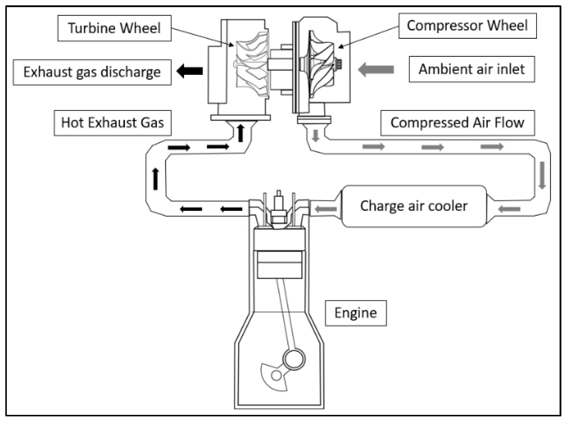
The schematic of a typical marine diesel engine is shown in Figure 1. A typical auxiliary diesel engine system powering ships’ systems and equipment comprises an internal combustion engine, turbocharger, charged air cooler, and other auxiliary systems for cooling and lubrication. The engine combusts the air and generates power. The exhaust gases are routed to the turbocharger where the expansion of the gases is used for rotating the turbine. The compressor attached to the turbine shaft compresses the air and supplies the charged air to the engine manifold for higher power generation. Malfunction of any of the engine components lowers the power generation capacity and, therefore, it is critical to monitor the condition of engines and subcomponents. Normally, the engine and subcomponents undergo scheduled maintenance after a specific number of operational hours prescribed by the manufacturer. Although, the scheduled maintenance provides longer operational life of engine, it normally results in over maintenance. A key challenge for the unscheduled maintenance of the engine and subsystems is the short window period available for inspection and repair at the port during cargo loading and unloading, and the unavailability of spare parts for the replacement. Therefore, a real-time monitoring anomaly detection and intelligent fault diagnosis tool is essential for predicting the impending failures and for better planning of the maintenance and procurement.

In the marine sector, vibration monitoring and oil analysis are widely used methods for fault diagnosis of diesel engines. Over the years, various vibration-based condition monitoring systems with different signal processing techniques were proposed for fault detection in diesel engines [3,4,5] and are suitable for identifying mechanical faults such as valve failure, unbalance, and bearing or gear failure in the diesel engines. However, the vibration signal is not useful for identifying faults associated with components having non-moving parts such as the air filter, intercooler, inlet, and exhaust manifold. Moreover, most of the works use a single vibration sensor to monitor the faults. However, it is necessary to measure the vibration at several locations and from multiple directions depending on the size of the machines and the fault location and employ data fusion techniques for accurate fault diagnosis [6].

Fault diagnosis approaches using thermodynamic data were proposed for identifying typical thermodynamic failures such as air filter clogging, intercooler clogging, engine misfire, valve failures, turbine and compressor fouling /clogging, leakages in inlet and exhaust manifolds, etc., in the diesel engines. Lamaris and Hontalas (2010) proposed a general-purpose diagnostic technique for marine diesel engines using a thermodynamic simulation model [7]. Rubio et al. (2018) developed an engine model using AVL Boost tool to obtain the response of diesel engines for typical failures without having to induce them in a real engine [8]. The simulator was able to generate symptoms of diesel engines for 15 failures, and the authors also proposed methodology to build a simulator for any diesel engine. Xu Nan et al. (2022) also carried out a similar study and developed an engine simulation model to replicate the influence of various faults on the performance of a marine diesel engine [9]. Cui, Xinjie et al. (2018) introduced a gas path diagnosis approach for the condition monitoring of a diesel engine turbocharger [10]. He, Zhichen et al. (2021) proposed a thermodynamic parameter-based performance indicator for the fault detection scheme in marine diesel turbocharging systems [11]. Xu, Xiaojian et al. (2021) published a more comprehensive review on the various fault diagnosis approaches in the marine systems, their limitations, and the research directions [12].

Various machine learning (ML)- and artificial intelligence (AI)-based condition monitoring and fault diagnosis tools were proposed in the literature for the marine diesel engines. Li, Zhixiong et al. (2012) presented a feasibility study for fault diagnosis of diesel engines using instantaneous angular speed. Authors used Support Vector Machines (SVM) for multi-class recognition of the marine diesel engine faults and achieved 94% accuracy in fault diagnosis [13]. Vibration signal was used for fault diagnosis of diesel engines by Porteiro, Jacobo et al. (2011) using Neural Networks [14] and by Gkerekos et al. (2016) using supervised learning [15]. Zabihi-Hesari, Alireza et al. (2019) used time and frequency domain features of the vibration signal from intake manifold and cylinder heads of diesel engine as input features to the neural network and achieved classification accuracy of 98.34% [16]. A hybrid fault diagnosis approach combining manifold learning and isolation forest was proposed by Wang, Ruihan et al. (2021) for accurate fault diagnosis of diesel engines [17]. Bai, Huajun et al. (2022) employed Stacked Sparse Autoencoder for dimensionality reduction in multi-sensor vibration data and used SVM for fault classification and achieved accuracy of 98% [18]. A more detailed review of the various ML and AI approaches for fault classification of diesel engines can be found in the literature [19].

Many works in the literature used the vibration signal for the fault diagnosis of diesel engines. Vibration signal is useful only for fault diagnosis of certain mechanical faults such as unbalance, valve malfunction, bearing faults, etc., and is not useful for diagnosis of faults affecting the thermodynamic performance. The accuracy of fault diagnosis is highly dependent on the vibration sensor location relative to the fault and the presence of nearby auxiliary equipment, and their operation influences the fault detection accuracy. Although multiple vibration sensors were used for the engine fault diagnosis [6], it is highly challenging in the case of fault diagnosis of auxiliary engines to isolate the fault, as multiple engines at different loads operate at the same time.

Thermodynamic data-based fault diagnosis of engines can detect a higher number of failures with better accuracy. However, it is worth noting that most of works in the literature that are based on the thermodynamic data utilize the simulation models to generate the failure data to avoid testing on a real engine. The accuracy of the simulation models is highly dependent on the tuning of various parameters in the models. The accuracy of model estimation varies from one load point to another load point for the same engine [8], and the effect of the faults on the engine performance could be in the same range as that of error from the simulation model. Furthermore, some works used data from experiments on a sophisticated and highly sensorized diesel engine test bench. However, the data available from the actual engines onboard the vessel is much less due to the limited number of sensors onboard. Only critical operational parameters are measured and displayed in the engine room. For instance, a mass flow sensor can clearly identify abnormal operations of either engine, compressor, or intercooler. However, it is too expensive to deploy a mass flow sensor on each of the engines. Similarly, it is not practical to measure accurately the maximum temperatures in the cylinder or the pulsating exhaust gas turbine inlet pressure. Fault diagnosis methodologies with minimum engine operational data as input need to be developed for practical implementation. Finally, fault simulation is carried out by varying the process parameters in the models [8,9,10]. For instance, the compressor failure is simulated by reducing the mass flow of air and the isentropic efficiency [9], and the fault diagnosis was carried out by quantifying the variation in other thermodynamic parameters. A real failure simulation on the actual engine instead of a simulation model would capture the effect of failures in a more realistic way, and such failure data is needed for developing the anomaly detection and fault diagnosis tools.

This article aims to present a comprehensive predictive maintenance framework for turbocharger systems, detailing the overall architecture encompassing sensorization of critical components, data acquisition, and edge computation processes, as well as the development of AI-based anomaly prediction and machine learning-driven fault diagnosis models.

This work, firstly, uses the actual operational data acquired from a 1.89 MW auxiliary diesel engine of a cargo vessel for the development of anomaly detection and fault diagnosis models. The healthy data of the engine was collected for two years, and the faults were induced on the actual engine to generate the failure data. As far as the knowledge of the author goes, such work has not been published in the literature. The novelty of the work also lies in using data fusion from both the thermodynamic parameters and vibration for the fault diagnosis instead using either of the data. The presented work acts as guideline for the development of fault diagnosis tools, throws light on the challenges, and showcases the benefit.

Although multi-sensor data have been explored in previous marine engine studies, most existing approaches rely on simulation environments or laboratory test benches with dense and idealized instrumentation. In contrast, real vessels operate under strict sensor, safety, and data-access constraints, resulting in sparse, noisy, and incomplete measurements. The key research gap addressed in this study lies in developing and validating AI-based anomaly detection and fault diagnosis models using multi-modal data collected directly from an in-service marine engine, where fault data are limited and operating conditions are highly variable. This distinction is critical for practical deployment, as models developed under controlled conditions often fail to generalize to real ship environments.

The structure of the paper is as follows. Firstly, the details of the predictive maintenance system of diesel engines, including sensorization and data acquisition, are presented. The details of the marine diesel engine on which the failure simulation is carried out is presented. Subsequently, the approach for inducing the failures with different severity levels on the engine is discussed. Thereafter, the details on the anomaly detection and fault diagnosis models are presented. Finally, the results are presented, discussed, and the conclusions are provided.

2. Condition Monitoring System for Marine Diesel Engines

2.1. Marine Diesel Engine System

The details of the marine diesel engine used for the monitoring and the fault diagnosis is presented in this section. The anomaly detection and fault diagnosis models are developed using the data acquired from the auxiliary engines of a container ship. The loading capacity of the container ship is 37,373 tonnes, and it was built in 2013. The container ship is equipped with a main diesel engine of rated power 23 MW, and two turbochargers were supplying the compressed air to the two inlet manifolds of main engine. Four units of diesel engine generator sets manufactured by Hyundai HiMSEN were installed onboard the container ship for the power generation. Each engine is 4-stroke, vertical and direct injection-type with a rated power of 1.89 MW, and operating at 900 RPM. Each auxiliary diesel engine is equipped with a turbocharger and an intercooler. The fault simulations were carried out one of the auxiliary diesel engines during the voyage.

2.2. Overview of Predictive Maintenance System

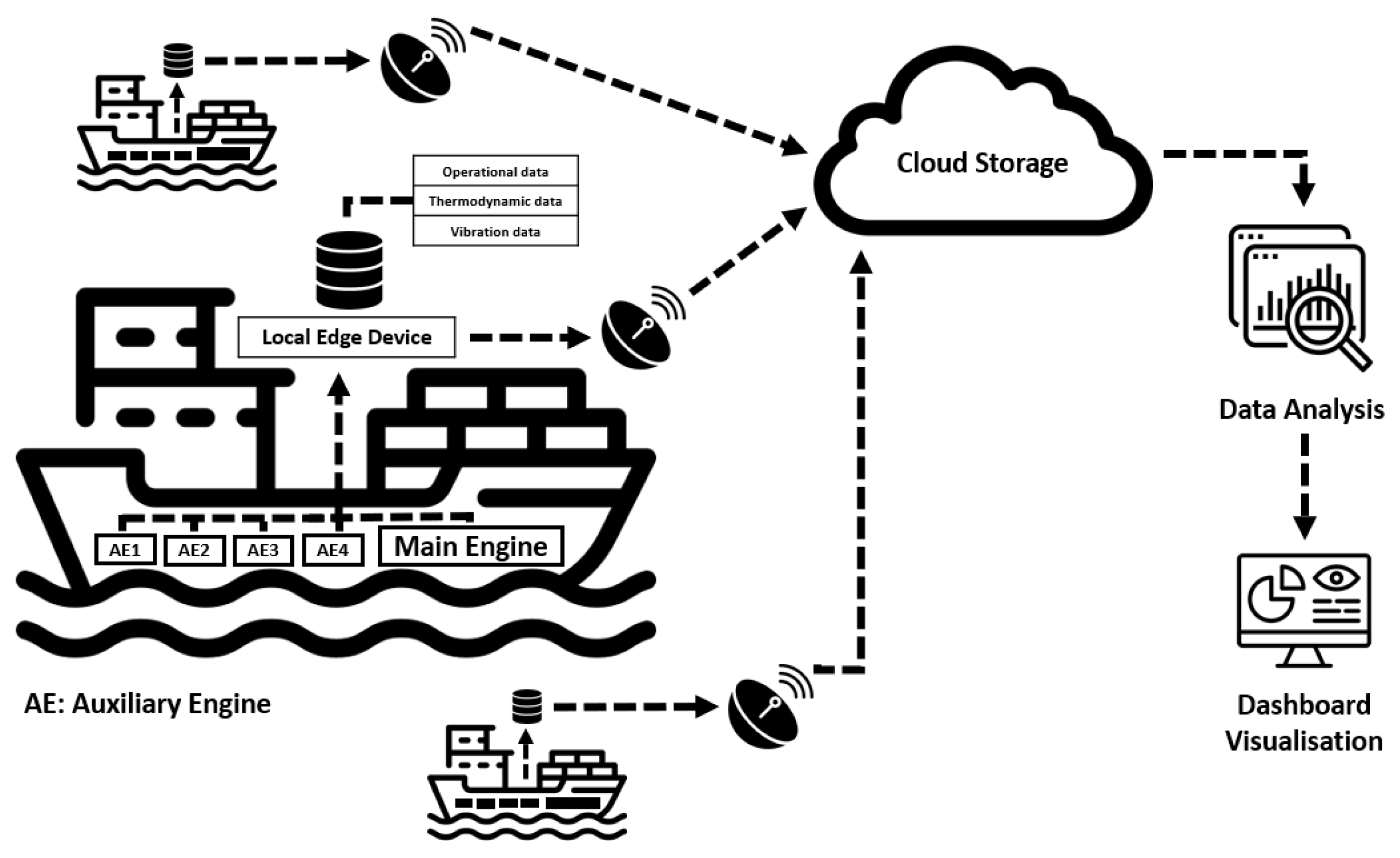
To develop predictive maintenance system capable of anomaly detection and fault diagnosis, the data from the main and auxiliary engines of several container vessels was collected over a period of two years. The schematic of the overall architecture of the system used for the data collection is presented in Figure 2. The operational data, the thermodynamic performance data, and the vibration data from all the engines was collected on an edge device onboard the vessel. The data was time synchronized, processed, and the important features of each engine system onboard the vessel were uploaded to the cloud storage through VSAT (very small aperture terminal) transmission. The data was analyzed for real-time anomaly detection and fault diagnosis using ML/AI algorithms. The data, metrics, and notifications were displayed on a web dashboard for asset performance monitoring and decision making by the fleet operators, managers, and the owners.

2.3. On-Board Data Acquisition Module

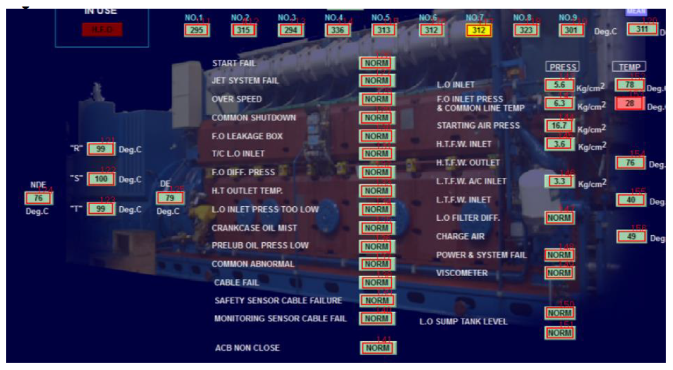
The acquired data comprises three different types of information of the engine system, namely operational data, thermodynamic performance data, and vibration data. The list of available parameters for each engine onboard the vessel is given in

Table 1. Data available for each engine.

Engine Parameters	Turbocharger Parameters
Engine generator status	Turbine inlet gas temperature
Engine RPM	Turbine outlet gas temperature
Engine load	Turbocharger speed
Voltage and Amperage	Bearing and lubrication system parameters
Charged air pressure	Lubrication oil pressure
Charged air temperature	Lubrication oil inlet temperature
Engine start pressure	Bearing temperature
Engine cylinder (1–6) temperatures	Cooling system parameters
Fuel injection system parameters	Cooling water pressure
Fuel oil pressure	Cooling water temperature (inlet and outlet)
Fuel oil temperature	Vibration
Fuel oil mass flow rate	Time series and frequency domain features

. The operational data of the engine includes engine load, speed, voltage, amperage, turbocharger speed, etc. The thermodynamic data includes the pressure and temperature at various points in the flow path of air and hot gas through the engine, turbocharger, and intercooler. Additionally, the pressure and temperature data of the engine supporting systems such as fuel injection, lubrication, and cooling systems are also available. The engine operational data and the thermodynamic data is normally displayed in the engine control room for the vessel crew to monitor the condition of all the engines. The displayed data was captured from the PC screen of the engine room in a non-intrusive manner using ADLINK’s DEX-100 (ADLINK Technology, Inc., New Taipei City, Taiwan) intelligent data extraction system [20]. The built-in frame grabber captures the engine control room screen display and processes the contents on the screen as shown in Figure 3 to acquire the data. The operational and thermodynamic data acquired from the screen of the engine control room is labelled and stored with timestamps on the edge device.

A single axis accelerometer was installed on each engine, and the vibration data was collected at a sampling rate of 20,000 Hz. The engine speed is 900 RPM (15 Hz), and its harmonics normally extend up to 500 Hz. However, the turbocharger rotates in the speed range of 20,000 to 40,000 RPM depending on the engine load. Therefore, the vibration data was collected at a very high sampling rate to also investigate the faults from the turbocharger. All the acquired data including operational, thermodynamic, and vibration data was locally stored in an edge device (Beckhoff CX5130, Beckhoff Automation GmbH & Co. KG, Verl, Germany) and time synchronized. The vibration data was stored for each minute, and the data was processed locally to generate useful features for the anomaly detection and fault diagnosis. The time-series features generated from the vibration signal include mean, root mean square (RMS), peak to peak, standard deviation, kurtosis, skewness, etc. The frequency domain features of the vibration data were generated from the Fast Fourier Transforms. The time-series and frequency domain features are computed on the edge device. The thermodynamic parameters and the vibration features were uploaded to the cloud through VSAT transmission. The anomaly detection and the fault diagnosis models were deployed in the cloud. The output from the models and important feature data is displayed in the web dashboard for real-time monitoring.

In practical shipboard environments, measurement noise, sensor drift, and intermittent data gaps are unavoidable due to vibration, thermal variation, sensor aging, and communication constraints. In this study, such effects were mitigated using standard engineering preprocessing measures, including signal smoothing, range validation based on manufacturer specifications, normalization against operating conditions, and exclusion of corrupted or incomplete data segments. Given that the investigated faults are gradual degradation mechanisms, short-term noise and minor data loss have limited impact on the diagnostic trends of interest. Image-based data extraction from control room displays was employed as a pragmatic solution when direct digital interfaces were unavailable, reflecting a common constraint in existing vessels [21]. To ensure stability, data capture was restricted to fixed screen layouts and steady operating conditions, with extracted values cross-checked against expected operating ranges. While this approach cannot match the fidelity of direct sensor interfaces, it provides sufficient reliability for monitoring long-term performance degradation, which is the focus of this study; a detailed uncertainty analysis and long-term interface comparison are therefore identified as future work.

3. Anomaly Detection and Fault Diagnosis Models

In this work, two models were developed, one for the anomaly detection and second for the fault diagnosis of the diesel engines. The intention behind developing two models is to serve two different purposes based on the availability of the data. The anomaly detection model is developed to deploy on the marine diesel engines without any previous failure data. The healthy data of the engine will be acquired for a pre-defined interval of time, and the anomaly model will be trained on that healthy data, and the model will be used for prediction of anomalies afterwards. The autoencoder (AE)-based anomaly model predicts the anomaly but will not provide information on the fault type. Therefore, a second model for fault diagnosis is proposed. The fault diagnosis model is developed for the scenario where the failure data is available. With the availability of failure data, the fault diagnosis can also be carried out with better accuracy. Usually, one marine vessel is equipped with multiple auxiliary engines for redundancy. The failure data acquired from one engine can also be used for developing fault diagnosis machine learning models of engines of similar models and with the same rated capacity. It should be noted that the failure data used in this paper is generated by inducing the faults on the diesel engine. The anomaly detection model is to notify the vessel crew or operator on the impending failure, and the fault diagnosis tool provides more specific information on the fault type.

3.1. Anomaly Detection Model

Over the years, many algorithms have been developed to detect anomalies across various applications, and Nassif, Ali Bou et al. (2022) provided a comprehensive review of the literature on the anomaly detection algorithms [22]. The neural network-based anomaly detection techniques have improved the accuracy of detection on the large and complex datasets, leading to the implementation in wide applications. Supervised, semi-supervised, and unsupervised anomaly detection algorithms were proposed for anomaly detection in a wide variety of real-world applications.

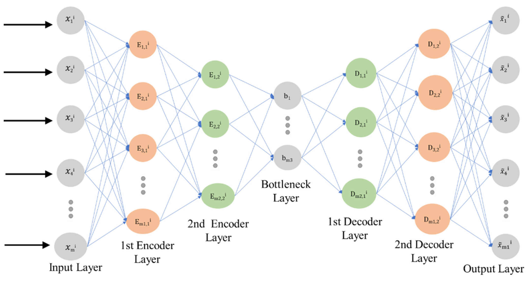
In this paper, unsupervised Stacked Autoencoder (SAE) is used for the detection of the anomalies from the data of auxiliary diesel engine. AE is a neural network-based unsupervised learning algorithm widely applied in data compression and denoising applications. Typically, an AE is composed of an encoder and a decoder, and each of them may contain single or multiple hidden layers. An AE with a single hidden layer is termed as undercomplete autoencoder (UAE), while the AE with many hidden layers is termed Stacked Autoencoder (SAE). AE maps the input data into latent representation at a reduced dimension in the encoding process and reconstructs the data in the decoding process and learns the distribution of the original data. Unlike many of the published works, the SAE in this paper was trained only with healthy engine data without labelling, and the limits of the reconstruction loss on the healthy data was established. The model learns the behaviour of a healthy diesel engine, and the reconstruction loss increases during the prediction when anomalies or some fault beginning to affect the health of engine are present. It should be emphasized that the anomaly detection model detects the anomaly but do not provide any information on the nature of the anomaly.

In this paper, stacked autoencoder is used for anomaly detection in the engine data. The schematic of SAE is shown in Figure 4. The encoder maps the input sensor data X = (x¹, x², x³, …, x^N) into a lower-dimensional representation through non-linear transformation along the hidden layers, and the decoder generates an estimation ($\tilde{X}$) of the input vector X. The input data X contains data from m sensors ($x_1^N$, $x_2^N$, $x_3^N$, … $x_m^N$) at each of N observations. The output of each encoder (E_i) and decoder ($D_i^{\prime }$) layer is given by

$$E_i={\sigma }_{\theta }^e(x, E_{i-1})$$

(1)

$$D_i^{\prime }={\sigma }_{\phi }^d(E_i, D_{i-1})\hspace{1em}\hspace{1em}\&\hspace{1em}\tilde{x}={\sigma }_{\phi }^d(D_i^{\prime })$$

(2)

where σ is the activation function. The functions θ and φ represent the parameter set for the encoder and decoder layers, respectively. Rectified Linear Unit (ReLU) was used as the activation function for both encoder and decoder layers. The input data of each layer is transformed to hidden representation through ReLU, and the output representation ($\tilde{X}$) is computed by minimizing the reconstruction error (${\Vert x-\hat{x}\Vert }^2$).

The stacked autoencoder (SAE) employed in this study is a deep unsupervised neural network that learns hierarchical feature representations of multivariate turbocharger sensor data. Each autoencoder layer aims to reconstruct its input by minimizing the mean squared reconstruction loss L = ${\Vert x-\hat{x}\Vert }^2$, where X is the input vector and $\hat{x}$ is its reconstruction. The encoder transforms the input through a non-linear activation function h = ReLU(W_ex + b_e), while the decoder performs the inverse mapping $\hat{x}$ = W_dh + b_d. By stacking multiple encoding–decoding layers and performing layer-wise pretraining followed by global fine-tuning, the SAE progressively captures higher-order correlations and non-linear dependencies within the turbocharger operating data, allowing it to model complex normal behaviour with high fidelity.

During training, the SAE is exposed only to data representing healthy turbocharger operation. This enables it to learn a compact latent representation of nominal system behaviour, effectively forming a manifold of normal conditions. When new data are passed through the trained model, the reconstruction error E = (1/n) ${{\sum }_{\mathrm{i}}}^{\mathrm{n}}{\Vert x_{\mathrm{i}}-{\hat{x}}_{\mathrm{i}}\Vert }^2$ serves as an anomaly score. Higher values indicate a deviation from the learned distribution and thus potential faults. To improve robustness, the ReLU activation constrains hidden features to non-negative values, encouraging sparsity and enhancing interpretability of latent features related to physical parameters such as shaft speed, temperature, and vibration amplitude. This formulation provides a theoretically grounded yet computationally efficient method for anomaly detection, demonstrating improved sensitivity to early degradation patterns compared with traditional linear approaches such as PCA or threshold-based statistical monitoring.

To quantitatively distinguish normal and abnormal operating conditions, the distribution of reconstruction errors from the training (healthy) dataset is modelled using a Gaussian fit E ~ $\mathcal{N}$(μ_E, σ_E²). An anomaly threshold T is then defined as T = μ_E + kσ_E, where k is a sensitivity constant empirically chosen between 2 and 3 to control the false-alarm rate. Data samples with E > T are flagged as anomalous. This probabilistic thresholding provides a statistically grounded decision criterion, ensuring that detected anomalies represent statistically significant deviations from the learned normal manifold. In the turbocharger application, this approach allows early detection of abnormal behaviours, such as imbalance or thermal drift, before they manifest as measurable faults.

In this paper, the ability of SAE in learning the patterns of the input data is showcased by comparison with UAE. While both the unsupervised autoencoder (UAE) and stacked autoencoder (SAE) aim to learn compact representations of input data without labels, their architectures and learning capacities differ significantly. The UAE typically consists of a single encoder–decoder pair, limiting its ability to capture complex non-linear relationships in high-dimensional data. In contrast, the SAE extends this concept by stacking multiple autoencoder layers, where the output of each encoder serves as the input to the next. This hierarchical structure allows the SAE to progressively learn deeper and more abstract features, making it more effective in modelling the multi-scale dependencies inherent in turbocharger signals. Consequently, the SAE demonstrates superior reconstruction accuracy and anomaly sensitivity compared to a shallow UAE, particularly when dealing with diverse operating conditions and subtle degradation patterns.

The input data of size 96,897 observations with 42 features was reduced to 32, 16, and 8 features successively using three hidden layers to maximize the anomaly detection. The detection accuracy of SAE and UAE is compared to show the capability of SAE in learning complex patters from the data.

3.2. Fault Diagnosis Model

Numerous ML algorithms have been developed and implemented for fault classification across a wide variety of applications. In this work, various existing models have been trained, tested, and had their accuracy in the fault classification investigated. The top five ML algorithms that have performed well in terms of accuracy in the fault classification are discussed briefly below.

Decision Tree: A Decision Tree is a hierarchical structure that makes decisions by recursively splitting the data based on the feature values. The algorithm selects the best feature to split the data at each node, aiming to maximize the information gain or minimize impurity. This process results in a tree-like structure that can be used for classification by traversing the tree from the root to a leaf node, where the class label is assigned.

Random Forest: Random Forest is an ensemble learning method that combines multiple decision trees to improve the classification performance. It works by constructing multiple Decision Trees using different subsets of the training data and the random feature subsets. The final prediction is made by aggregating the predictions of individual trees, often resulting in more accurate and robust classifications compared to a single Decision Tree.

Extreme Gradient Boosting (XG Boost): XG Boost is a powerful gradient boosting algorithm that focuses on creating a strong ensemble of weak learners, usually Decision Trees. It optimizes a loss function through the iterative addition of trees, with each new tree correcting the errors made by the previous ones. XG Boost uses gradient descent and regularization techniques to prevent overfitting and achieve high predictive accuracy in classification problems.

Support Vector Machine (SVM): SVM is a supervised learning algorithm that seeks to find a hyperplane that separates different classes in the data in the best possible way by maximizing the margin between the classes. It works well for both linearly separable and non-linearly separable data by using kernel functions to transform the data into a higher-dimensional space. SVM aims to classify new instances by their position relative to the decision boundary.

K-Nearest Neighbour (KNN): KNN is a simple instance-based learning algorithm that classifies new data points based on the class labels of their K nearest neighbours in the training dataset. It measures the similarity between the instances using distance metrics (such as Euclidean distance) and assigns the majority class among the neighbours to the new data point. KNN’s effectiveness depends on the choice of K and the relevance of nearby instances.

Although several standard machine learning algorithms were evaluated for fault diagnosis, the contribution of this work lies not in the algorithms themselves but in how they are systematically adapted and integrated for turbocharger fault detection. Specifically, the proposed framework emphasizes (i) feature engineering from real operational signals tailored to mechanical fault patterns, (ii) uniform preprocessing and normalization to ensure fair inter-model comparison, and (iii) an interpretable evaluation pipeline that links model output with physical fault modes. This approach highlights how conventional algorithms can be effectively optimized for domain-specific diagnostics, demonstrating that accurate and explainable fault classification can be achieved even under limited labelled data—a key practical challenge in real-world turbocharger monitoring.

Existing AI- and machine learning-based fault diagnosis studies in the marine domain are predominantly based on simulation data, test-bench experiments, or densely instrumented systems. While these approaches demonstrate promising performance under controlled conditions, their applicability to real vessels is often limited by simplified modelling assumptions, impractical sensor requirements, and the scarcity of labelled fault data. In particular, gradual fouling-related faults exhibit weak and overlapping signatures that are easily masked by operational variability and sensor noise in real-world environments. As a result, the performance and robustness of many existing methods remain uncertain when deployed using the sparse sensor data typically available onboard. This gap motivates the present study, which focuses on evaluating fault diagnosis under realistic operational constraints using real-vessel measurements.

For the above-mentioned ML algorithms, the accuracy, and the balanced accuracy of the classification on test dataset and the cross-validation accuracy are compared, and the results are discussed.

4. Failure Simulation on Diesel Engines

Two failure modes, namely nozzle ring clogging and intercooler clogging, were induced in one of the auxiliary diesel engines onboard the vessel. The focus on nozzle ring blockage and intercooler blockage is motivated by their practical relevance and diagnostic difficulty in real marine operations. Based on technical discussions with industry practitioners, these two fault modes are among the most commonly encountered degradation mechanisms in service and can be safely induced under controlled operating conditions in in-service vessels. Importantly, these were the only fault scenarios approved by the ship’s Chief Engineer for experimentation, ensuring compliance with safety, operational, and regulatory constraints during onboard data collection. While large-scale statistical fault databases from operating vessels are rarely publicly available, particularly for commercial marine engines, fouling-related degradation in turbocharging and charge-air systems is widely recognized as a persistent operational issue. Both faults develop gradually due to fouling and contamination, leading to subtle performance deterioration rather than abrupt failures. This progressive behaviour makes early diagnosis particularly challenging when relying on limited and noisy onboard measurements and therefore aligns well with the objective of this study to investigate fault diagnosis using sparse real-vessel sensor data rather than high-fidelity laboratory instrumentation.

The failure simulations were carried out with increasing severity to generate useful failure data, to develop anomaly detection and fault diagnosis models, and to test the performance of the models. The details of the failure simulation are described below.

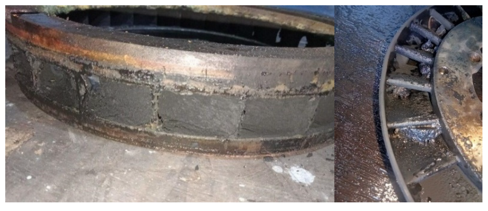
Nozzle ring clogging: Nozzle ring is a critical part of the turbine section of turbocharger, and its function is to direct the hot gas of the engine exhaust onto the turbine blades through its channels. The nozzle ring creates a narrow, high-velocity jet of exhaust gas to strike the turbine wheel at an angle, causing it to spin. Nozzle ring is the most frequently serviced component of the turbocharger because of the depositions formed in its channels. Generally, the marine diesel engines use marine fuel oil or heavy fuel oil for power generation and propulsion. The exhaust of the engine contains soot, and a solid layer of dirt forms on the nozzle ring when hot gas passes through the turbocharger. The pictures of clogged nozzle rings are shown in Figure 5. Such deposits of dirt in the nozzle ring lead to reduced mass flow in the diesel engine system and hot gas pressure build-up before the nozzle ring. Nozzle ring clogging not only decreases the efficiency of the turbine but also lowers power output of the engine and increases the fuel consumption.

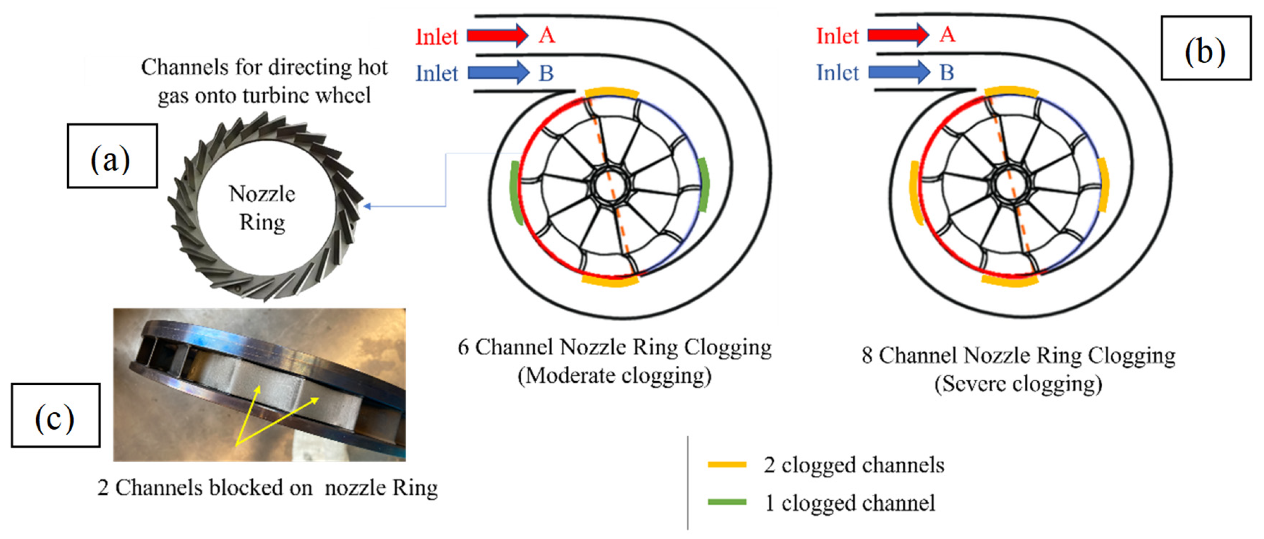
The turbocharger of the diesel engine comprises a twin-entry radial turbine which has two entries, one at the top (entry A) and a second at the bottom (entry B) to direct the hot gas from the engine exhaust on to the turbine as shown in Figure 6a. Usually, the clogging is more severe at the entrance of hot gas into the nozzle ring. The nozzle ring has 24 channels, and the clogging in the nozzle ring is simulated by blocking the channels. During the nozzle ring clogging simulation conducted on the vessel, four, six, and eight channels were blocked as shown in Figure 6b to simulate increasing severity of the clogging. The channels of the nozzle ring were blocked with metallic sheets as shown in Figure 6c. Three severity levels of nozzle ring clogging were indued during the failure simulation, namely low, moderate, and severe. The severity in the clogging was increased by increasing the number of blocked channels. A total of 4, 6, and 8 channels were blocked during the nozzle ring failure simulation and are termed as low, moderate, and severe nozzle ring clogging based on the percentage of blocked flow area on the nozzle ring. In the subsequent figures and analysis, the labels low NRC, moderate NRC, and severe NRC are used for identifying different levels of nozzle ring clogging.

Inter-cooler clogging: During the long operational time of intercooler, the air passages of the intercooler can be clogged or blocked. When the air passages of intercooler are blocked, the pressure builds up on the compressor side and reduces on the engine side. Therefore, the mass flow to the engine reduces. The temperature of the scavenged air entering the engine also increases due to intercooler clogging. Due to the above changes, the performance of engine and turbocharger is adversely affected. In the experiments, the intercooler clogging was simulated by reducing the flow area of the pipe supplying the charged air to the engine manifold by installing an additional gasket with reduced inner diameter. Three severity levels of intercooler clogging were induced in the failure simulation, namely low, moderate, and severe corresponding to 20%, 40%, and 60% blocking of flow area. For instance, to simulate 40% blocking, an additional gasket that covers 40% of the total flow area was installed in the flow path. In the subsequent figures and analysis, the labels low ICC, moderate ICC, and severe ICC are used for identifying different levels of intercooler clogging. The failure simulations of nozzle ring clogging and intercooler clogging were carried out at auxiliary engine loads of 825 kW, 900 kW, and 975 kW using heavy fuel oil.

The simulated faults were designed to replicate partial degradation mechanisms commonly observed in service, rather than destructive or safety-critical failures. In particular, the induced nozzle ring and intercooler blockages represent reversible fouling conditions consistent with early- to mid-stage degradation, ensuring physical relevance while maintaining operational safety. All fault simulations were conducted with approval from the ship’s Chief Engineer and were fully removed after testing, with the turbocharger system restored to its original configuration. Engine operation during the experiments remained within manufacturer-recommended limits, and no long-term impact on engine integrity was observed. The selected load conditions correspond to the most frequently encountered operating points during normal vessel operation, as confirmed through consultation with onboard engineering personnel. These operating points serve as representative sampling locations that capture the dominant engine behaviour relevant to condition monitoring. While dynamic load transients and extended load coverage may provide additional insights, they were intentionally excluded to minimize operational risk and experimental complexity and are identified as directions for future work.

5. Results and Discussion

In this section, the results of the work are discussed. Firstly, the failure data analysis is presented and compared with the baseline data to investigate the influence of faults on the engine performance. Subsequently, the results of the anomaly detection and the fault diagnosis model are presented.

Table 2. Diesel engine healthy and failure data counts.

Parameter	Count
Total number of data	96,897
Healthy data	95,594
Anomalous data	1303
Total number of clogged nozzle ring data	658
Low clogged nozzle ring data	311
Moderately clogged nozzle ring data	226
Severely clogged nozzle ring data	122
Total number of clogged intercooler data	644
Low clogged intercooler data	168
Moderately clogged intercooler data	297
Severely clogged intercooler data	179

provides the count of the data points used in this study. The size of the dataset is 96,897 data points out of which the failure data amounts to 1.3% only. Therefore, the accuracy of anomaly detection and fault diagnosis models needs to be high to avoid false positives and false negatives.

5.1. Data Analysis

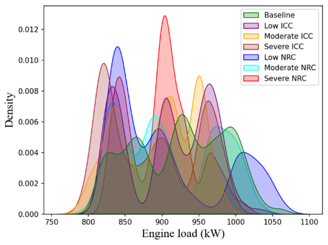
The engine load is taken as reference for the failure simulation and for comparison between the healthy and failure data. The distribution of the engine load data for the baseline (or healthy) and the failure simulation are plotted in Figure 7. The failure simulation was carried out at mean engine loads of 825 kW, 900 kW, and 975 kW, which is less than 50% of engine rated power. A baseline was also carried out at the same engine loads before simulating the faults for the better comparison of the data. It can be clearly seen from the figure that most of the peak densities of the different failure simulation data points are matching with 825 kW, 900 kW, and 975 kW. A few of the data points, for instance low NRC failure simulation, are slightly deviating from the reference engine loads. It is very difficult to maintain the constant load on the engine as the power requirement from various auxiliary systems onboard the vessel varies and, therefore, the engine load varied during the failure simulation experiments. The influence of failures on the key thermodynamic parameters is discussed below. The baseline data in the following graphs refers to the data collected from healthy engine just before conducting the failure simulation. Note that for the anomaly detection and fault diagnosis models, the healthy data refers to the entire data collected over the two years. In Section 5.1, firstly, the parameters upstream of the engine and followed by parameters at the exhaust are compared and discussed.

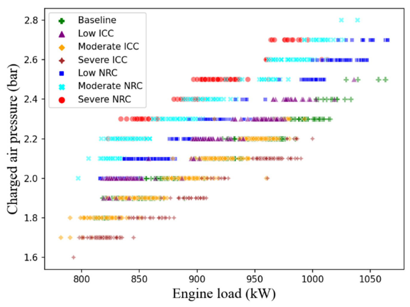
The intercooler reduces the temperature of the pressurized hot air from the compressor before passing to the engine inlet manifold as shown in Figure 1. The charged air pressure is measured at the outlet of the intercooler before the engine inlet manifold and is plotted in Figure 8. Note that the resolution of the pressure data is 0.1 bar and, therefore, only significant changes in the charged air pressure can be captured. The charged air pressure reduces when the intercooler is clogged compared to the baseline value or healthy state as shown in the figure. When the severity of ICC is low, the deviation of the charged pressure is minimum from the healthy state. The higher the severity of the clogging, the lower is the charged air pressure and higher the deviation from the baseline value. In the case of nozzle ring clogging, the pressure before the turbine increases because of the clogged nozzle ring channels. However, the pressure at the turbine inlet is not measured. But, the back pressure in the engine exhaust due to the nozzle ring clogging increases the pressure in the engine inlet manifold to maintain the mass equilibrium. Therefore, the charged air pressure increases due to the nozzle ring clogging when compared to the healthy state as shown in the figure. At 975 kW of engine load, the charged air pressure increased significantly by 0.4 bar when the nozzle ring was severely clogged.

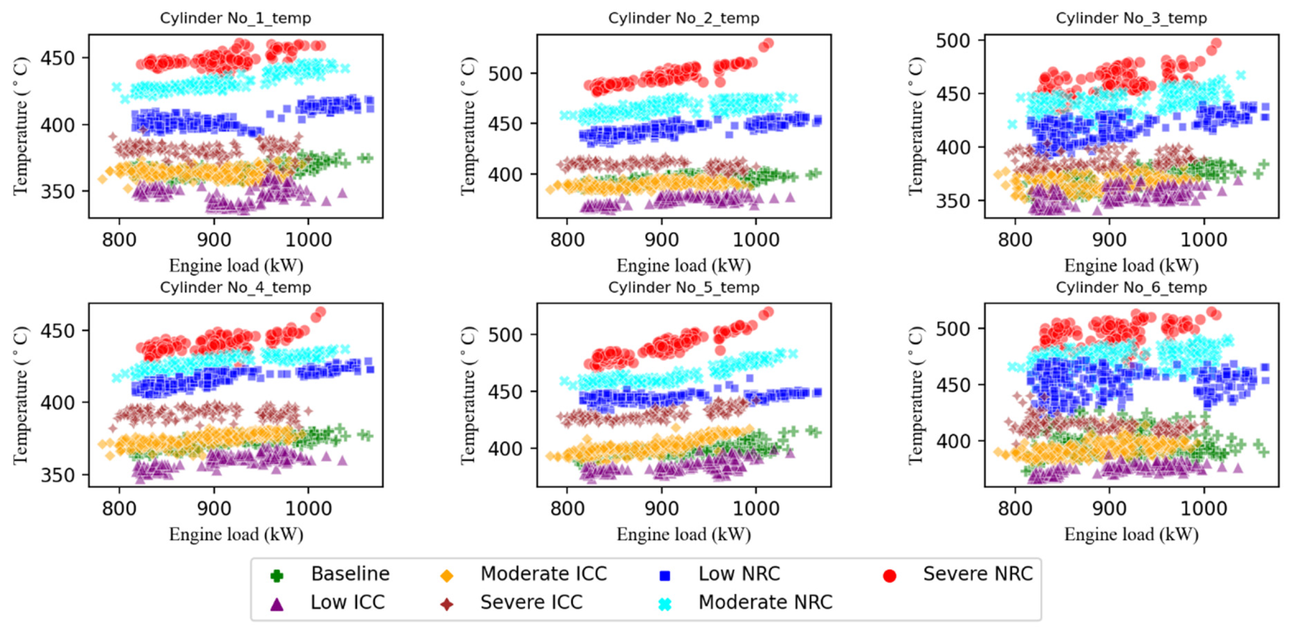
The exhaust gas temperatures at the outlet of each of six cylinders is plotted in Figure 9. When either the intercooler or the nozzle ring is clogged, the mass flow rate of the air or hot gas across the diesel engine system reduces and therefore the output power of the engine reduces. The engine injects additional fuel into the cylinders to generate additional power to meet the load requirement. The rich fuel/air mixture results in higher combustion temperatures and, therefore, the temperature measured at the outlet of each cylinder is increased as shown in Figure 9. The effect of nozzle ring clogging is much higher on the cylinder exhaust temperatures when compared to the intercooler clogging. Severe NRC increases the cylinder temperatures significantly in the range of 60 to 80 °C. From the plot, it can be observed that the cylinder exhaust temperatures gradually increase with the severity of the fault, and this pattern can be used for the anomaly detection and quantifying the fault. For intercooler clogging, the increase in the cylinder exhaust temperature is much lower compared to the nozzle erring clogging. It is due to the selected engine load range for the failure simulation. The failure simulations were carried out at 40–50% of rated engine load. Therefore, when the intercooler is clogged by low to moderate levels, the flow area is sufficient for the air to flow from the intercooler to the engine manifold without affecting the engine performance. The influence of the intercooler clogging on the engine performance is significant only when the clogging is severe, and the cylinder exhaust temperatures increased due to the additional fuel injection by the engine.

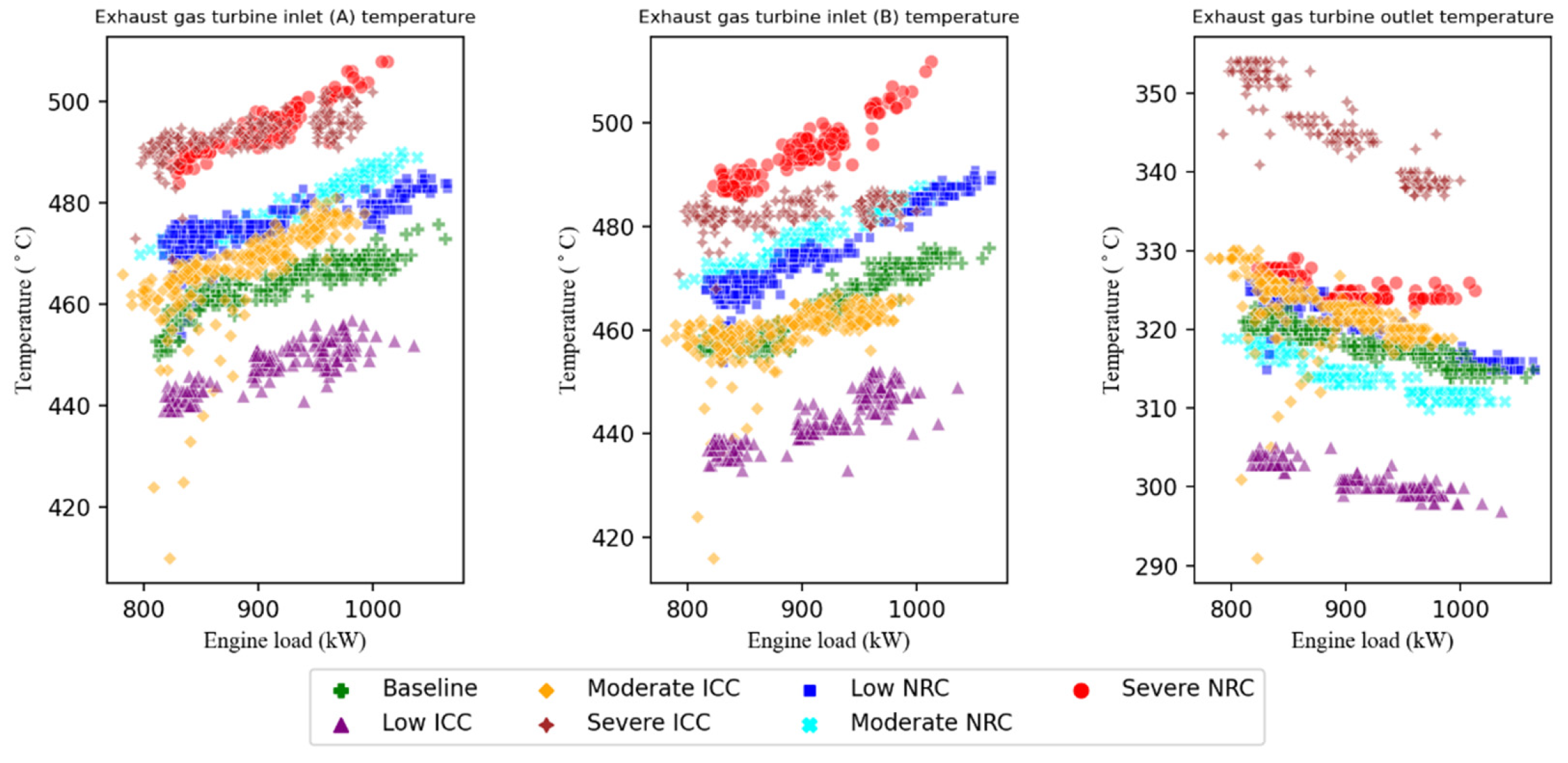
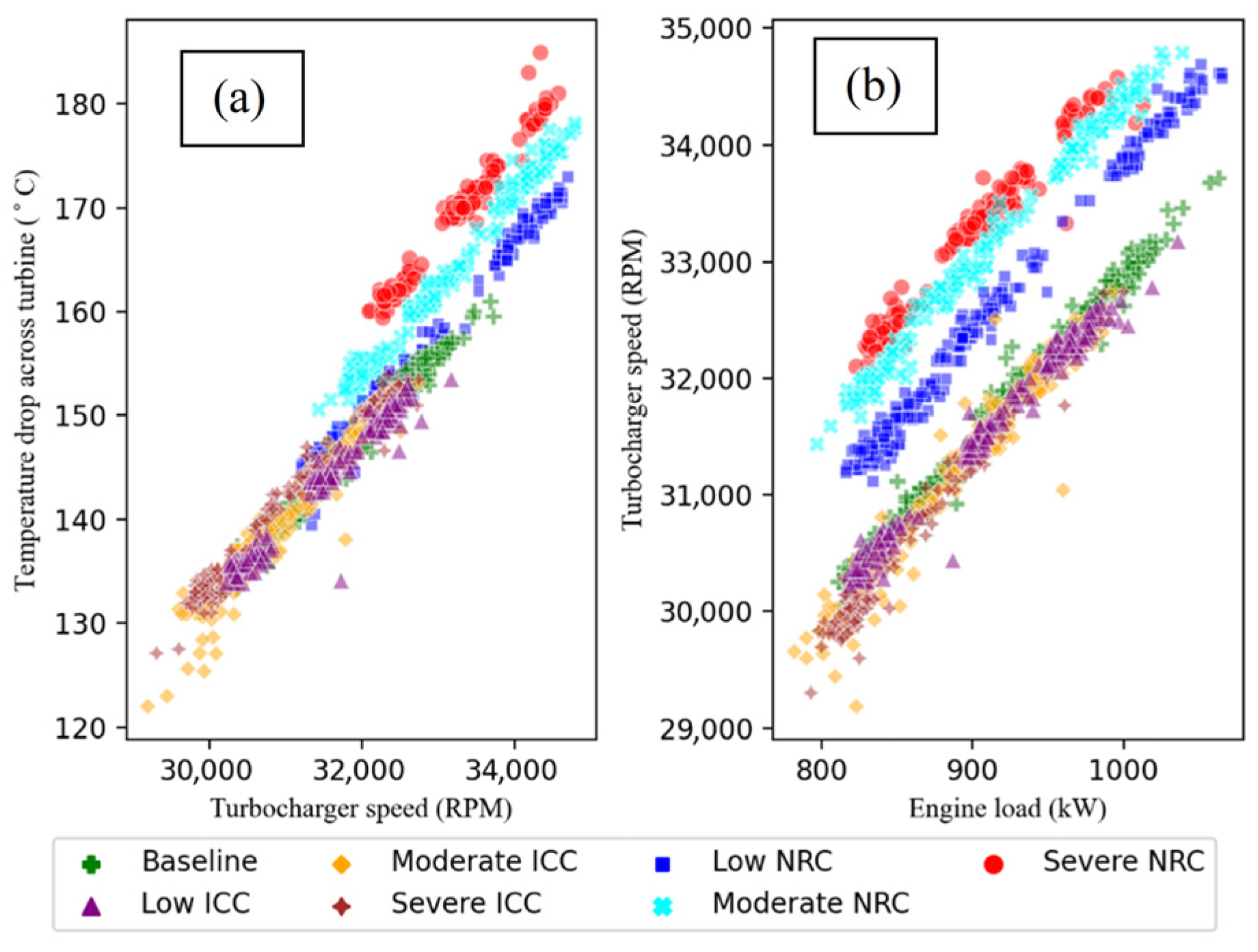
The diesel engine was equipped with a twin-entry radial turbocharger, and the exhaust gas inlet temperatures measured at both entrances of the turbine and the turbine exhaust outlet temperature are plotted in Figure 10. When the cylinder exhaust temperatures increase due to the additional fuel injection, the turbine inlet temperatures also increase. For nozzle ring clogging, the turbine inlet temperatures increase while the turbine outlet temperature remains the same, indicating higher temperature differential across the turbine as shown in Figure 11a. Higher temperature differential indicates higher enthalpy change and more work done. For the turbine to spin at the same speed, higher temperature drop across the turbine is required when the nozzle ring is clogged, indicating the faulty and less efficient operation. A similar observation can also be noticed from Figure 11b where the turbine speed is plotted versus engine load. To generate the same load, the turbine is spinning at higher speeds with the clogged nozzle ring. When the intercooler is clogged, the turbine outlet temperature increased along with the inlet temperature. The temperature difference across the turbine, i.e., the work done, is essentially same as the healthy state as shown in Figure 11a,b.

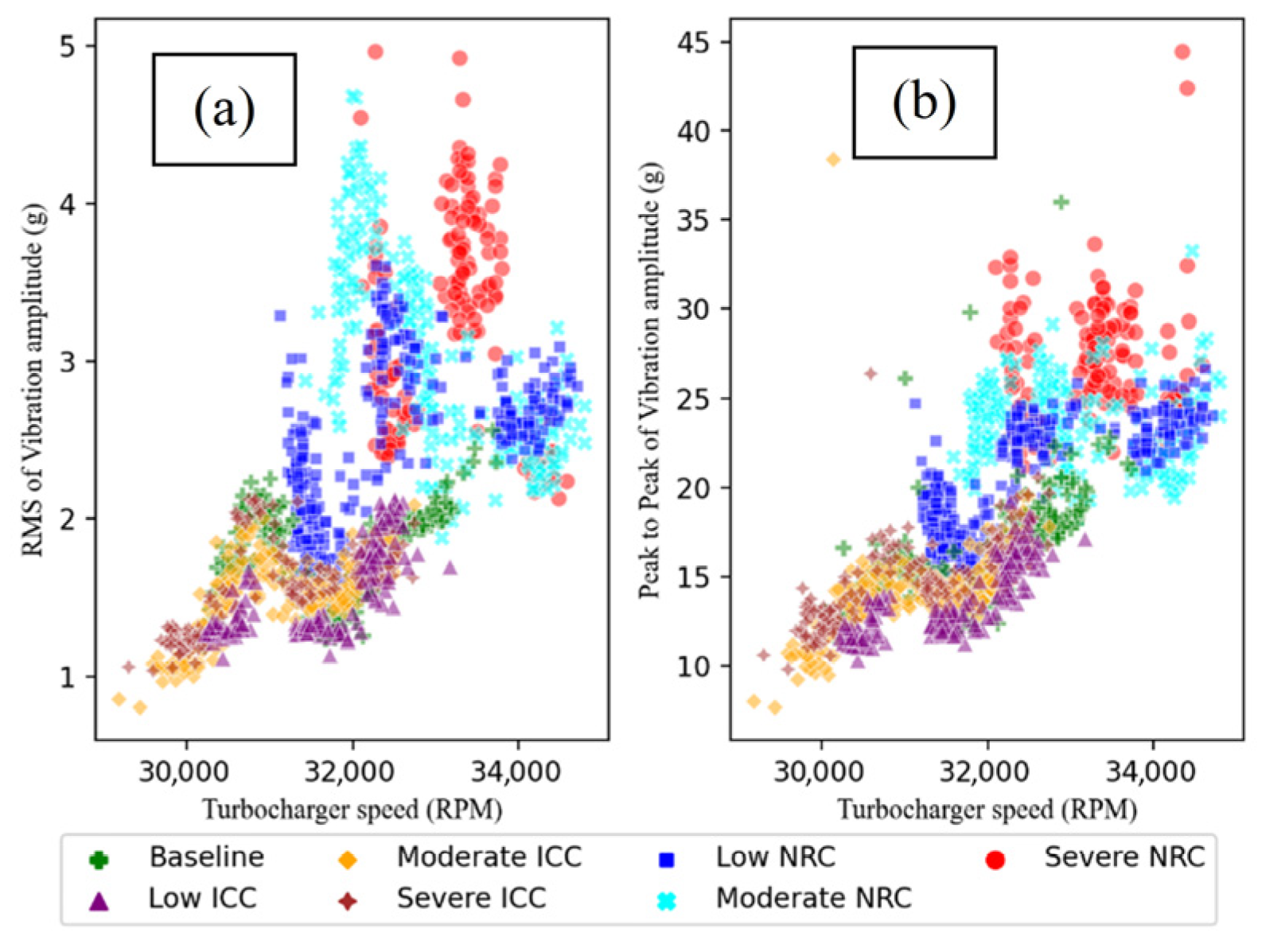
The time-series and frequency features from vibration signal are useful for the anomaly detection and the fault diagnosis of mechanical faults. The time series features used in this work include root mean square (RMS), peak to peak, standard deviation, etc., and the frequency features include the vibration energy at 1× rotational frequency of the turbocharger computed from Fast Fourier Transform with Power Spectral Density (PSD) of the vibration signal. The Power Spectral Density (PSD) is used to quantify how vibration energy is distributed across frequencies, providing a consistent measure of signal power independent of time-domain variations. In turbocharger diagnostics, monitoring the PSD at the 1× rotational frequency helps identify increases in vibration energy that signal rotor imbalance or bearing wear. Unlike raw vibration amplitude, PSD offers a normalized view that allows reliable comparison across different operating speeds and conditions. Hence, it serves as a robust indicator for tracking mechanical health over time. The RMS and peak to peak of the vibration signal are plotted in Figure 12a and Figure 12b, respectively. It is evident from the plot that the RMS and peak to peak increased significantly due to the nozzle ring clogging, whereas the intercooler clogging has minimum influence. The nozzle ring clogging directly influences the rotation of the turbine and excites the engine harmonics and, therefore, the RMS and peak-to-peak vibration amplitude increased significantly. However, the intercooler is a static component, and its clogging narrows the flow path of the air but will not affect either the reciprocating motion of the engine or the rotation of the turbine wheel. Therefore, the vibration features did not vary much for the case of intercooler clogging. It should be noted that although the RMS and peak-to-peak vibration amplitude are increased, it is difficult to infer the root cause of the fault from the vibration feature pattern alone, unlike the thermodynamic data. It can also happen that the RMS and peak-to-peak vibration amplitude might increase because of another fault machinery situated near to the diesel engine. Therefore, it is difficult to diagnose the fault with vibration time-series features alone.

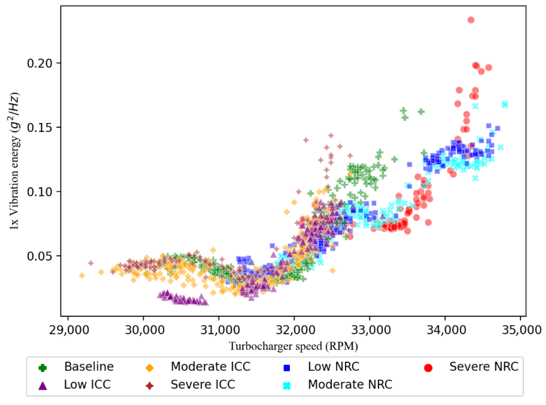
The vibration energy at 1× rotational frequency is plotted in Figure 13 and is very useful for investigating unbalance in the rotating components such as the turbine shaft, turbine wheel, and compressor wheel. The vibration energy is the integrated value of the amplitudes computed from Fast Fourier Transform over a 20 Hz frequency band with the central frequency of 1× rotation frequency of turbocharger. Figure 13 suggests that 1× vibration energy levels did not vary during intercooler and nozzle ring clogging simulations. The result is expected as the failure is not induced by any of the rotational components of the turbocharger. Note that the vibration levels of intercooler clogging are overlapping with the baseline data. However, the nozzle ring failure simulation data points are clearly operating at higher turbocharger speed when compared to the baseline data. The reason is that the turbocharger with a clogged nozzle ring operates at much higher speed to supply compressed air for the engine to generate the same load.

Although many other parameters of auxiliary systems are available in the data, the influence of faults on those parameters is minimum. The insights from this section are very useful in understanding the trend of various parameters when the intercooler and nozzle ring clogging failure happens.

5.2. Anomaly Detection Results

Undercomplete autoencoder (UAE) with a single hidden layer and stacked autoencoder (SAE) consisting of multiple hidden layers are used for the detection of the anomalies from the data of auxiliary diesel engine. The SAE with multiple hidden layers learns complex features from the dataset in a much better way than the UAE model. The dataset contains 42 features and is compressed successively during the encoding process. For the UAE model, the 42 features are compressed to 8 features in the latent space using a single hidden layer. For the SAE model, 42 features are compressed in a sequency of 32, 16, and 8 in three hidden layers of the encoding process. For training the autoencoder models, 80% of the healthy data of the auxiliary diesel engine collected over the years is used for the training the model. The remaining 20% of healthy data and the failure data from the simulated experiments on the auxiliary engine of the vessel is used for testing the accuracy of anomaly detection. The parameter values of the learning rate, batch size, and epochs were optimized to achieve the best possible accuracy of the models. The optimized values for the learning rate, batch size, and epochs are 0.001, 16, and 50, respectively.

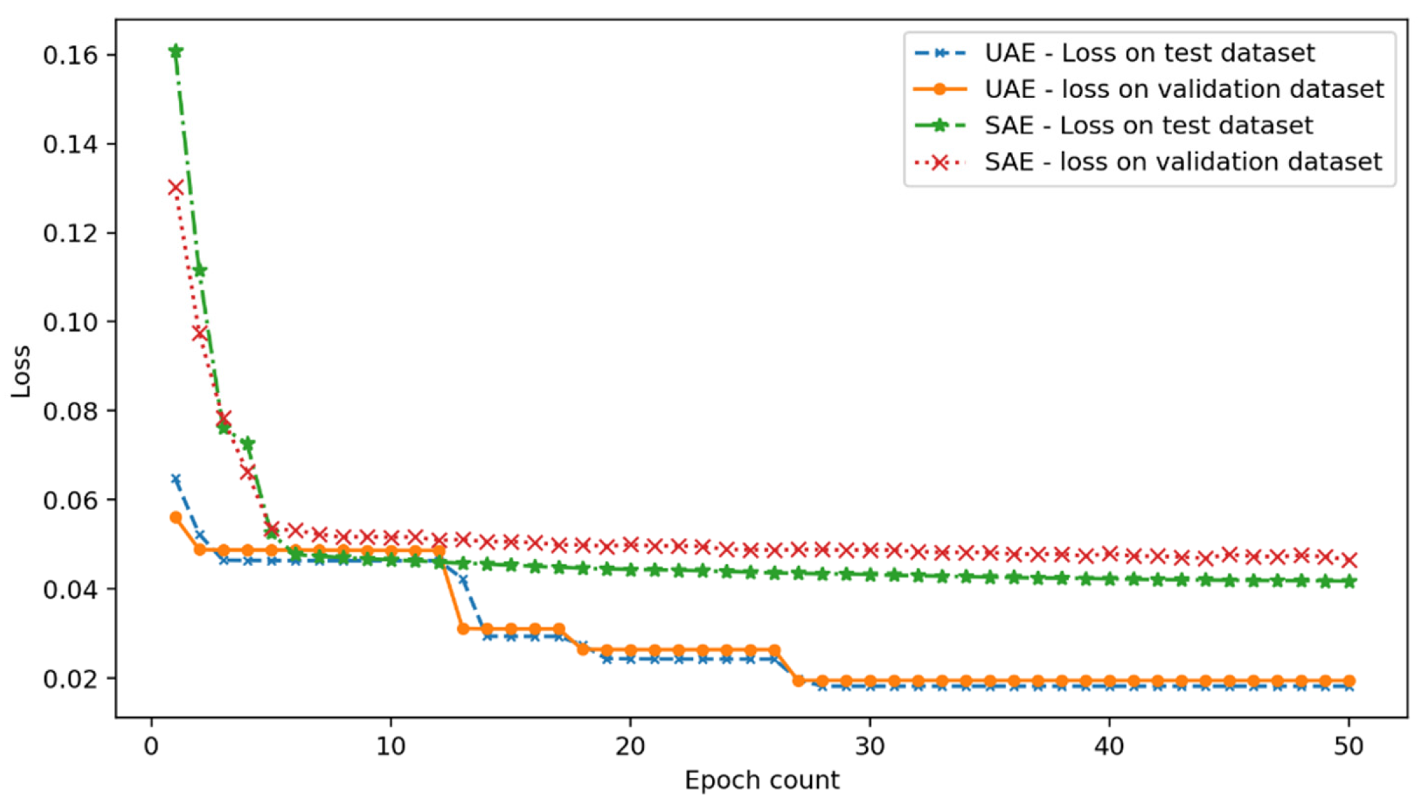
The loss between the input data (X) and the estimation ($\tilde{X}$) of the input vector from the decoder is minimized during the training process. The training and validation data loss computed during the successive epochs is plotted in Figure 14. The convergence is achieved quite early in the training process of SAE, and the loss remained constant for the remaining epochs. The convergence for the UAE model is gradual and achieved around 30 epochs of training. Similar values of loss on the validation dataset and the training dataset suggests the models are fitted well without either underfitting or overfitting.

Usually, the performance of different models is compared based on the accuracy. The accuracy is defined as percentage of instances where the predicted label matches with the true label of the observation. However, the accuracy is not a very good indicator of the model performance for the highly imbalanced datasets, such as those used in this work, where the healthy data is a very high portion of the dataset. The fault data is only 1.3% of the entire dataset. For highly imbalanced sets, the balanced accuracy and F1 score are very good indicators of the model performance. The balanced accuracy is defined as the average of recall obtained in each class where recall is the ratio of true positives to the total number of data points belonging to that class. F1 score is defined as the geometric mean of precision and recall. Precision refers to the number of true positives divided by the total number of positive predictions. The values of accuracy, balanced accuracy, and F1 score from UAE and SAE models in predicting different anomalies are given in

Table 3. Evaluation metrics of anomaly detection models.

	Undercomplete Autoencoder	Stacked Autoencoder
Nozzle ring clogging faults
Accuracy	99.83	99.70
F1 Score	97.55	95.72
Balanced accuracy	99.69	99.84
Intercooler clogging faults
Accuracy	96.70	98.09
F1 Score	6.04	63.10
Balanced accuracy	51.55	75.00
Combined faults
Accuracy	96.79	98.15
F1 Score	67.36	83.84
Balanced accuracy	75.90	87.57

.

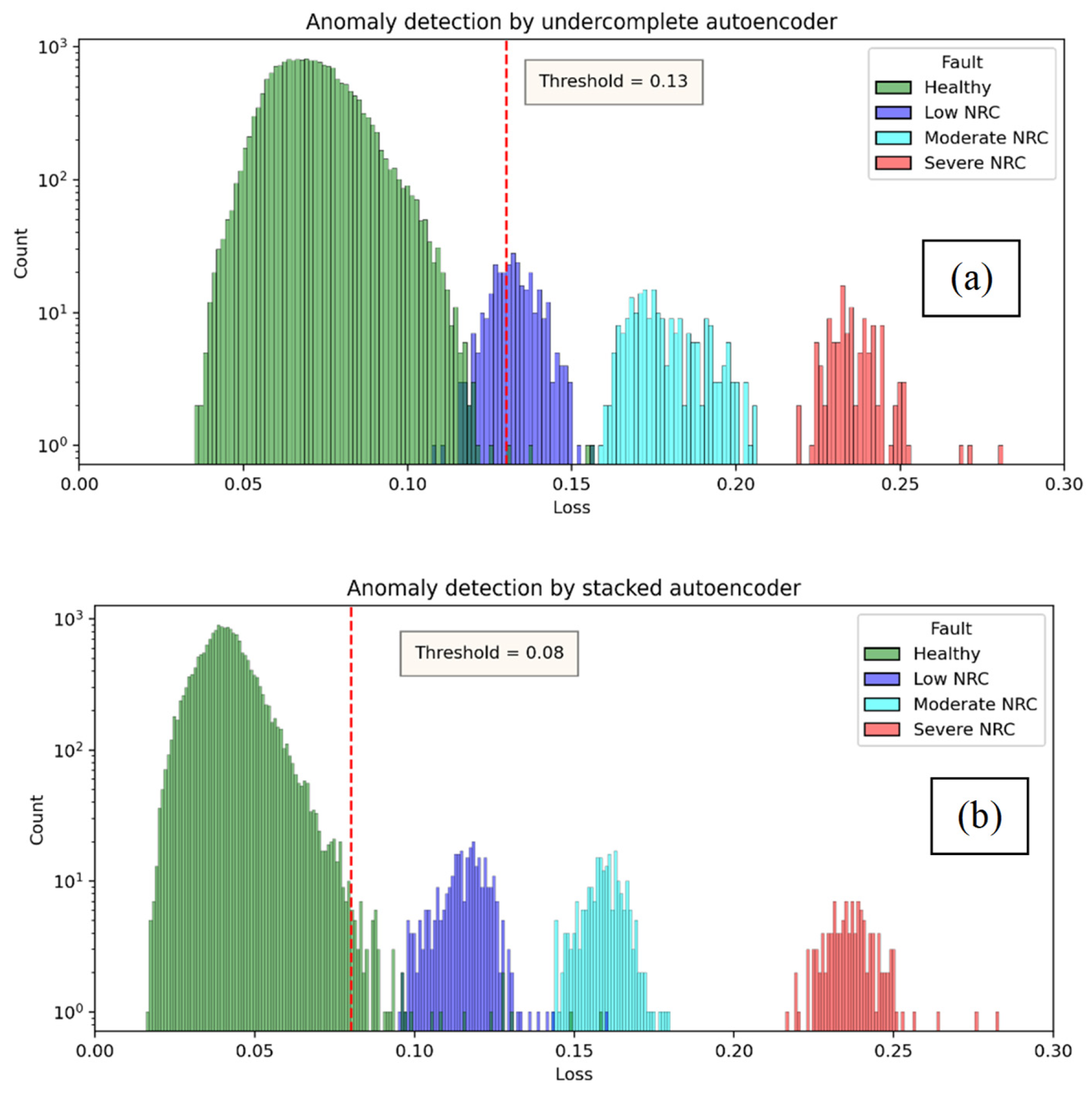
The reconstruction loss computed on the test dataset with Nozzle Ring Clogging (NRC) failures using UAE and SAE models is plotted in Figure 15 and labelled in colours according to its factual healthy or anomaly severity condition. Reconstruction loss thresholds were then selected based on UAE and SAE models prediction results that distinguish healthy and anomaly condition. The upper threshold for reconstruction loss on the healthy data is taken as 0.13 and 0.08 for UAE and SAE models, respectively, and are marked as vertical dotted lines as shown in the figure. These thresholds differentiate healthy and anomaly condition based on UAE and SAE models’ prediction results. When the reconstruction loss from any observation is beyond the thresholds, the observation is predicted as the anomaly by the models. For the nozzle ring clogging failure simulation, the influence on the various engine parameters is very significant and, therefore, the anomalies are clearly distinguished from the healthy data points by both the UAE and SAE models. As the severity of nozzle ring clogging increases, the reconstruction loss moves further away from the threshold clearly distinguishing the anomaly. UAE and SAE models are predicting nozzle ring clogging anomalies with accuracies of 99.8% and 99.7%, respectively. The balanced accuracy from both the models is above 99% and is very good. The F1 score of the UAE and SAE models is 97.5% and 95.7%, respectively. The performance metrics indicate that the nozzle ring clogging is very distinguishable and anomaly prediction by both the models is very good. In fact, the UAE model is performing slightly better than the SAE.

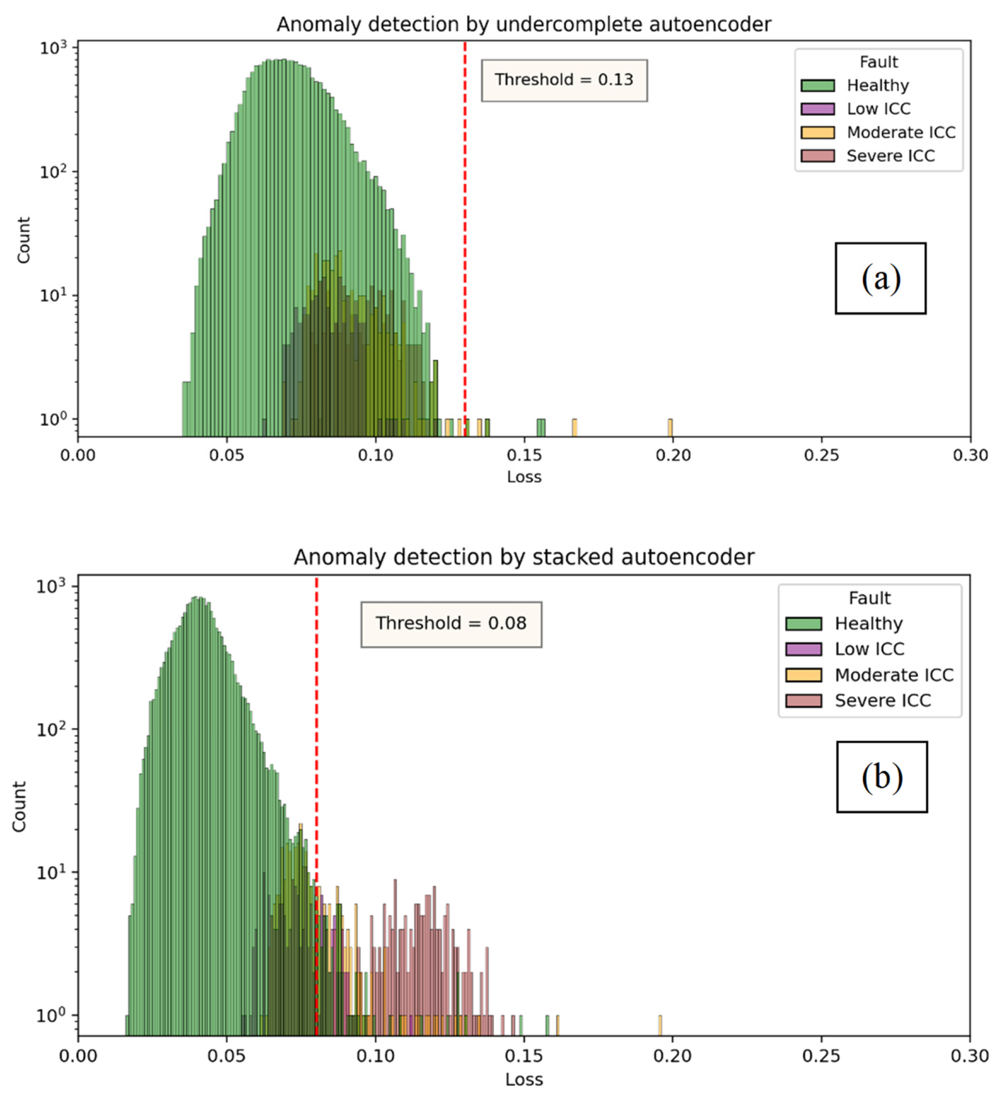
For the intercooler clogging failure simulation, the reconstruction loss from the UAE and SAE is plotted in Figure 16. From Section 5.1, it can be observed that the deviation of thermodynamic parameters is not significant from the baseline for the intercooler clogging. Therefore, it is very difficult to predict the anomalies accurately, as it can be seen that there is significant overlap between healthy and anomaly prediction by the UAE model, as shown in Figure 16a. The UAE model predicts most of the intercooler failure data as healthy data resulting in a very poor F1 score of 6% and balanced accuracy of 51.5%. It is observed from the data analysis section that the deviation of thermodynamic parameters is not significant for low ICC and moderate ICC. But severe ICC shows significant deviation from the baseline as shown in Section 5.1. However, the UAE model could not classify any of low, moderate, and severe ICC as anomalies, and the reconstruction loss is predicted in the range of healthy data. Therefore, the balanced accuracy and F1 score of the UAE model is very poor. However, SAE performs much better compared to the UAE and predicts intercooler anomalies very well with an accuracy of 63.1%. The reconstruction loss from SAE model in predicting ICC failure is shown Figure 16b. Moderate ICC and severe ICC were well separated from the healthy data when compared to low ICC failure data. The intercooler clogging case shows the ability of SAE to detect anomalies from the complex dataset. The F1 score and the balanced accuracy of SAE model in predicting ICC faults is 63.1% and 75%, and the values are much better than the UAE model. Prediction of low ICC failures is very difficult as the severity is not significant enough to affect the engine performance.

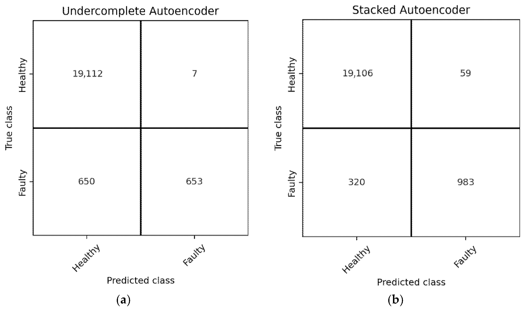
The overall accuracy of the UAE and SAE combining both the nozzle ring and intercooler clogging failures is shown as confusion matrix in Figure 17. The overall accuracy of the UAE and SAE is 96.8% and 98.1%, respectively. UAE wrongly predicts 650 instances of anomalies out of 1303, whereas SAE predicts 320 wrongly out of 1303. F1 score of the UAE and SAE models is 67.4% and 83.8%, respectively. The balanced accuracy of the UAE and SAE models is 75.9% and 87.6%, respectively. The results clearly indicate that the SAE is a much more powerful tool for anomaly detection compared to UAE. The unsupervised anomaly detection models such as SAE are very useful for identifying growing faults in the engines and perform necessary maintenance or repair.

Analysis of misjudgement cases indicates that most incorrect detections occur during early-stage degradation, where fault-induced parameter variations overlap significantly with normal operational fluctuations. This behaviour is inherent to gradual fouling-related faults and reflects the practical difficulty of distinguishing incipient degradation from healthy operation using sparse onboard measurements. The superior performance of the stacked autoencoder (SAE) over the undercomplete autoencoder (UAE) in intercooler clogging detection can be attributed to its higher representational capacity, which enables more effective modelling of complex correlations among thermodynamic and air-handling parameters affected by charge air flow restriction. In contrast, the UAE exhibits limited ability to capture such coupled non-linear relationships. Regarding vibration data, the measured signals remained largely similar across healthy and fault conditions, as the investigated faults primarily influence gas flow and thermal processes rather than inducing pronounced mechanical excitation. Consequently, vibration features provided limited additional discriminative information in this study. These finding highlights that the benefit of multi-source data fusion is fault dependent; while vibration signals are valuable for mechanically driven faults such as imbalance or bearing degradation, their contribution to diagnosing fouling-related air-path faults is inherently limited. The results therefore emphasize the importance of selecting sensing modalities based on underlying fault mechanisms rather than assuming universal benefit from data fusion.

The stacked autoencoder (SAE) in this study is employed for anomaly detection rather than direct feature attribution or fault classification. As such, the learned latent representation captures deviations from normal operating behaviour across multiple correlated engine parameters instead of assigning explicit importance rankings to individual features. Different fault mechanisms affect different subsets of parameters; therefore, a global feature importance ranking is neither meaningful nor physically representative for the considered faults. Instead, the relevance of specific measurements, such as cylinder exhaust temperature or charge air pressure, should be interpreted in the context of the corresponding fault mechanism. For fouling-related faults affecting the turbocharging and air-handling systems, variations in exhaust temperature are consistent with known thermodynamic behaviour due to changes in air–fuel ratio and exhaust energy utilization. To evaluate diagnostic behaviour, confusion matrices were analyzed with fault types aggregated by mechanism, illustrating how the SAE-based anomaly detection distinguishes between different fault categories rather than severity levels. The observed misclassifications reflect overlapping fault signatures and gradual degradation characteristics, which are inherent challenges in real-vessel condition monitoring.

The generalization capability of the proposed framework is therefore assessed at the fault-type level, rather than across unseen fault mechanisms or severity levels. The objective of this study is not to develop a universal fault classifier, but to evaluate whether anomaly detection trained on healthy operation can reliably differentiate between major fouling-related fault categories using sparse onboard sensor data. Generalization to unseen fault types or finer severity differentiation would require additional fault-specific data and is identified as future work.

5.3. Fault Diagnosis Results

The anomaly detection model presented in the previous section is useful when the failure data is lacking. When the failure data is available, very accurate and useful fault diagnosis models can be developed to predict the type of the fault, and such models are very useful for the predictive maintenance of engines and subsystems. As mentioned earlier, various existing supervised ML algorithms were trained using both the labelled healthy and failure data acquired from the diesel engine. The dataset is labelled taking into consideration the severity levels for both intercooler clogging and nozzle ring clogging failures. There are a total of seven classes, namely healthy, low ICC, moderate ICC, severe ICC, low NRC, moderate NRC, and severe NRC. The entire dataset is divided into training and testing data in the ratio of 80% and 20%, respectively. Various models were trained on the training dataset, and their performance in prediction of multi-label classification problem is investigated in terms of accuracy and balanced accuracy. The accuracy is calculated on two sub-portions of the original dataset. First, on a portion of the training dataset, which is called K-fold validation, where K refers to the number smaller sets or folds the training data is divided into. The training is carried out on K-1 folds and tested on the remaining fold and the process is looped, and the average accuracy on the validation set is computed [23]. Secondly, the accuracy of prediction on the test dataset is computed and reported. The accuracy of various algorithms on the cross-validation and training datasets in the prediction of multi-label classification is given. Most of the ML algorithms are performing very well, with more than 99% accuracy on the test dataset and cross-validation dataset. However, the high accuracy is due to the highly imbalanced dataset where the majority of the datapoints represent the healthy class, with very few datapoints (1.3%) representing the failure data. Therefore, another metric named as the balanced accuracy is used for evaluating the accuracy of imbalanced datasets. The balanced accuracy is a more reliable metric for evaluating the algorithms developed using highly imbalanced data. The balanced accuracy is a fair representation of a model’s performance as it accounts for both majority (healthy) and minority classes (all faulty). The balanced accuracy given in

Table 4. Comparison of different machine learning algorithms for diesel fault diagnosis with different severity levels.

Machine Learning Algorithm	Accuracy (%)	Accuracy (10-Folds Cross Validation, %)	Balanced Accuracy (%)
SVM Linear Kernel	99.99	99.98	99.72
XG Boost	99.99	99.99	99.11
Random Forest	99.98	99.99	98.78
Decision Tree	99.97	99.97	97.99
K-Nearest Neighbour	99.86	99.76	92.32

and is sorted in descending order based on the values of the balanced accuracy. The table shows that SVM algorithm performs better than other ML algorithms with 99.7% balanced accuracy. XG Boost algorithm also performs very well with a balanced accuracy of 99.1%. Random Forest and Decision Tree algorithms are both tree-based classification algorithms and give balanced accuracies of 98.8% and 98%, respectively. Random Forest algorithm combines the outputs from multiple decision trees to predict the class, and therefore it has better accuracy than the Decision tree algorithm. K-Nearest Neighbours shows the lowest accuracy of 92.3%. KNN can perform much better when the different classes of the data are clearly distinguishable.

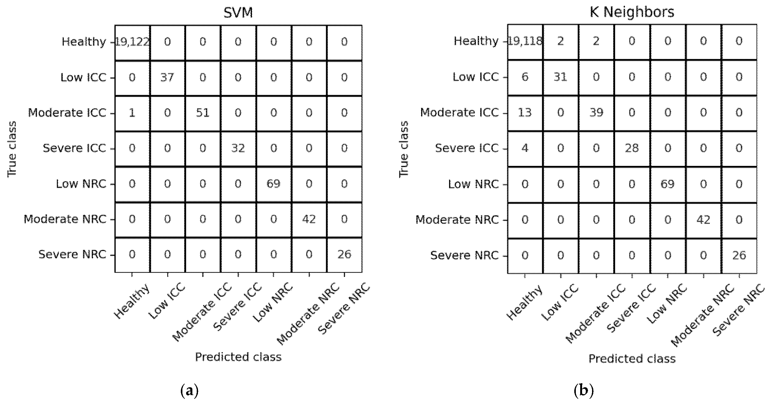
The balanced accuracy can be understood in a better way using the confusion matrix given in Figure 18 from the SVM and KNN algorithms which are the best and the worst performing algorithms, respectively. It can be clearly seen that the count of healthy data points is very huge when compared to the failure data and, therefore, the overall accuracy of all the algorithms is very high. SVM correctly predicts 19,122 instances corresponding to baseline class with 100% accuracy. The accuracy is 100% for all the classes except for moderate ICC. Generally, SVM provides better accuracy when the data is linearly or non-linearly separable. From the data analysis section and anomaly detection results, it is noticeable that NRC failure data is very distinguishable from the healthy data. Therefore, SVM predicts all the NRC fault data accurately. Although, ICC failure data is less separated from the healthy data, SVM predicts different classes of ICC severities more accurately than the other algorithms. Only 1 out of 52 instances of moderate ICC are wrongly classified by SVM.

KNN classifies 4 instances out of 19,122 healthy counts as faulty. The accuracy of the KNN algorithm is poor particularly for classifying ICC faults. Some of the low, moderate, and severe ICC fault data points are wrongly classified as healthy. All the NRC fault data points are accurately classified by the KNN algorithm. The better performance of the KNN algorithm for NRC fault classification over ICC fault classification is because of the higher influence of NRC on the thermodynamic parameters when compared to ICC. When the deviation of data is higher from the healthy state, the algorithms can classify accurately.

Ten key features identified from the top five algorithms given in Table 4 are the cylinders (1–6) exhaust temperatures, the turbine inlet and exhaust temperatures, charged air pressure, and engine start pressure. Vibration features would be more important for the failures such as the engine valves failures, piston failures, turbocharger unbalance, etc. In summary, the SVM algorithm outperforms other classification algorithms and provides very high accuracy in fault diagnosis of a diesel engine. XG Boost and Random Forest also provide very good accuracy in fault classification. More data corresponding to other failures is needed to build a robust fault diagnosis model. The critical challenge in building the model is lack of failure data and, therefore, it is imperative to generate the failure data on the operational engine for building accurate models. Although the present study focused on using both the healthy and failure data from the same engine for the anomaly detection and fault diagnosis, it is possible to use the transfer learning approaches to deploy a model trained on one engine to the other engines. Moreover, as the data from multiple engines across number of vessels is collected, the amount of failure data increases and the accuracy of the anomaly detection and fault diagnosis models can be further improved.

6. Conclusions

The paper presented the development of the anomaly detection and fault diagnosis models for marine diesel engines. The purpose of the anomaly detection and fault diagnosis models is early detection of failures and isolation of fault to the critical components for optimized scheduling of the maintenance and for cost savings. The AI/ML models were developed with real operational data from the marine diesel engines deployed on the vessel. The failure data was generated by inducing the intercooler and nozzle ring faults on the operational diesel engine during the voyage. The thermodynamic and vibration data collected from the engine was used for the development of AI/ML models. It is observed that the influence of nozzle ring clogging on the engine performance is much more severe than the intercooler clogging. The unsupervised stacked autoencoder anomaly detection model has performed much better with an overall accuracy of 93.6% when compared to the undercomplete autoencoder. The supervised fault diagnosis model using SVM algorithm predicts the faults with varying severities with a very good accuracy of 99.7%. The key features identified for the accurate fault diagnosis are the cylinders exhaust temperatures, the turbine inlet and exhaust temperatures, charged air pressure, and engine start pressure. The important features for the fault diagnosis developed in this study indicate that the thermodynamic data is critical for the fault diagnosis and anomaly detection. Many studies used vibration signal for the fault diagnosis. However, the vibration features are useful for augmenting the performance of the anomaly detection and fault diagnosis models but cannot distinguish various faults on their own. Although various data from the auxiliary systems such as cooling and lubrication are available, the features could not contribute to the anomaly prediction or the fault diagnosis. The developed AI/ML models have significant potential to deploy across various applications involving diesel engines.

Despite the encouraging results, several limitations should be acknowledged. First, fault data represent a very small proportion of the overall dataset, reflecting the inherent rarity of fault events in real vessel operation. Second, the present study focuses on two fouling-related fault mechanisms, and the proposed framework is not intended to provide universal coverage of all engine or turbocharger faults. Third, model transferability across different engine types or vessels has not been explicitly addressed, as the study prioritizes feasibility evaluation under realistic onboard constraints rather than cross-platform generalization. Future work will therefore focus on expanding fault datasets through longer-term monitoring and controlled fault induction, as well as investigating transfer learning and domain adaptation strategies to improve robustness across engines with similar configurations. From an application perspective, integration of the proposed approach into ship operation and maintenance workflows will involve coupling anomaly detection outputs with maintenance logs, trend-based decision support, and gradual deployment within existing condition monitoring systems, enabling practical adoption without requiring extensive additional instrumentation.

References

1. IMO. Fourth Greenhouse Gas Study 2020. www.imo.org. Available online: https://www.imo.org/en/OurWork/Environment/Pages/Fourth-IMO-Greenhouse-Gas-Study-2020.aspx (accessed on 8 September 2023).
2. The Swedish Club. 2018. Available online: https://www.swedishclub.com/media_upload/files/Loss%20Prevention/Main%20Engine%20Damage/TSC-main-engine-WEB2020.pdf (accessed on 8 September 2023).
3. Li, Z.; Yan, X.; Yuan, C.; Peng, Z.; Li, L. Virtual Prototype and Experimental Research on Gear Multi-Fault Diagnosis Using Wavelet-Autoregressive Model and Principal Component Analysis Method. Mech. Syst. Signal Process. 2011, 25, 2589–2607. [Google Scholar] [CrossRef]
4. Zhao, H.; Zhang, J.; Jiang, Z.; Wei, D.; Zhang, X.; Mao, Z. A New Fault Diagnosis Method for a Diesel Engine Based on an Optimized Vibration Mel Frequency under Multiple Operation Conditions. Sensors 2019, 19, 2590. [Google Scholar] [CrossRef] [PubMed]
5. Xi, W.-K.; Li, Z.; Tian, Z.; Duan, Z. A Feature Extraction and Visualization Method for Fault Detection of Marine Diesel Engines. Measurement 2018, 116, 429–437. [Google Scholar] [CrossRef]
6. Li, Z.; Yan, X.; Guo, Z.; Zhang, Y.; Yuan, C.; Peng, Z. Condition Monitoring and Fault Diagnosis for Marine Diesel Engines Using Information Fusion Techniques. Electron. Electr. Eng. 2012, 123, 109–112. [Google Scholar] [CrossRef]
7. Lamaris, V.T.; Hountalas, D.T. A General Purpose Diagnostic Technique for Marine Diesel Engines—Application on the Main Propulsion and Auxiliary Diesel Units of a Marine Vessel. Energy Convers. Manag. 2010, 51, 740–753. [Google Scholar] [CrossRef]
8. Pagán Rubio, J.A.; Vera-García, F.; Hernandez Grau, J.; Muñoz Cámara, J.; Albaladejo Hernandez, D. Marine Diesel Engine Failure Simulator Based on Thermodynamic Model. Appl. Therm. Eng. 2018, 144, 982–995. [Google Scholar] [CrossRef]
9. Xu, N.; Zhang, G.; Yang, L.; Shen, Z.; Xu, M.; Chang, L. Research on Thermoeconomic Fault Diagnosis for Marine Low Speed Two Stroke Diesel Engine. Math. Biosci. Eng. 2022, 19, 5393–5408. [Google Scholar] [CrossRef] [PubMed]
10. Cui, X.; Yang, C.; Serrano, J.R.; Shi, M. A Performance Degradation Evaluation Method for a Turbocharger in a Diesel Engine. R. Soc. Open Sci. 2018, 5, 181093. [Google Scholar] [CrossRef] [PubMed]
11. He, Z.; Yang, Y.; Han, H.; Wang, J.; Zhang, Y.; Li, H. A key performance indicator-based fault detection scheme for marine diesel turbocharging systems. J. Frankl. Inst. 2021, 358, 9346–9363. [Google Scholar] [CrossRef]
12. Xu, X.; Yan, X.; Yang, K.; Zhao, J.; Sheng, C.; Yuan, C. Review of condition monitoring and fault diagnosis for marine power systems. Transp. Saf. Environ. 2021, 3, 85–102. [Google Scholar] [CrossRef]
13. Li, Z.; Yan, X.; Yuan, C.; Peng, Z. Intelligent Fault Diagnosis Method for Marine Diesel Engines Using Instantaneous Angular Speed. J. Mech. Sci. Technol. 2012, 26, 2413–2423. [Google Scholar] [CrossRef]
14. Porteiro, J.; Collazo, J.; Patiño, D.; Míguez, J.L. Diesel Engine Condition Monitoring Using a Multi-Net Neural Network System with Nonintrusive Sensors. Appl. Therm. Eng. 2011, 31, 4097–4105. [Google Scholar] [CrossRef]
15. Gkerekos, C.; Lazakis, I.; Theotokatos, G. Ship machinery condition monitoring using vibration data through supervised learning. In Proceedings of the International Conference of Maritime Safety and Operations 2016, Glasgow, UK, 13–14 October 2016; pp. 103–110. [Google Scholar]
16. Zabihi-Hesari, A.; Ansari-Rad, S.; Shirazi, F.A.; Ayati, M. Fault Detection and Diagnosis of a 12-Cylinder Trainset Diesel Engine Based on Vibration Signature Analysis and Neural Network. Proc. Inst. Mech. Eng. Part C J. Mech. Eng. Sci. 2018, 233, 1910–1923. [Google Scholar] [CrossRef]
17. Wang, R.; Chen, H.S.; Guan, C.; Gong, W.; Zhang, Z. Research on the Fault Monitoring Method of Marine Diesel Engines Based on the Manifold Learning and Isolation Forest. Appl. Ocean. Res. 2021, 112, 102681. [Google Scholar] [CrossRef]
18. Bai, H.; Zhan, X.; Yan, H.; Wen, L.; Yan, Y.; Jia, X. Research on Diesel Engine Fault Diagnosis Method Based on Stacked Sparse Autoencoder and Support Vector Machine. Electronics 2022, 11, 2249. [Google Scholar] [CrossRef]
19. Aliramezani, M.; Koch, C.R.; Shahbakhti, M. Modeling, Diagnostics, Optimization, and Control of Internal Combustion Engines via Modern Machine Learning Techniques: A Review and Future Directions. Prog. Energy Combust. Sci. 2022, 88, 100967. [Google Scholar] [CrossRef]
20. AdLink. Available online: https://www.adlinktech.com/Products/IoT_solutions/Smart_Factory/DEX-100 (accessed on 9 March 2025).
21. Ando, T. Pulsation and Vibration Measurement on Stator Side for Turbocharger Turbine Blade Vibration Monitoring. Int. J. Turbomach. Propuls. Power 2020, 5, 11. [Google Scholar] [CrossRef]
22. Nassif, A.B.; Talib, M.A.; Nasir, Q.; Dakalbab, F.M. Machine Learning for Anomaly Detection: A Systematic Review. IEEE Access 2021, 9, 78658–78700. [Google Scholar] [CrossRef]
23. SciKit-Learn. 3.1. Cross-Validation: Evaluating Estimator Performance—Scikit-Learn 0.21.3 Documentation. Scikit-Learn.org. Available online: https://scikit-learn.org/stable/modules/cross_validation.html (accessed on 8 September 2023).
Figure 1. Schematic of marine diesel engine system.
Information 17 00016 g001
Figure 2. Architecture of predictive maintenance system.
Information 17 00016 g002
Figure 3. Image processing technique to extract the operational and thermodynamic data of engine from the screens of engine control room.
Information 17 00016 g003
Figure 4. Schematic of stacked autoencoder model.
Information 17 00016 g004
Figure 5. Heavily fouled nozzle rings.
Information 17 00016 g005
Figure 6. (a) Typical nozzle ring. (b) Schematic of twin-entry radial turbine and locations of clogged channels. (c) Clogged nozzle ring used in experiments.
Information 17 00016 g006
Figure 7. Distribution of the engine load for the baseline data and the failure data.
Information 17 00016 g007
Figure 8. Impact of faults on the charged air pressure supplied to the engine inlet manifold.
Information 17 00016 g008
Figure 9. The influence of the fault on the cylinder exhaust temperatures. Auxiliary engine has six-cylinder configuration, and the number of each cylinder is added in the graph.
Information 17 00016 g009
Figure 10. The influence of the fault on the radial turbine inlet and outlet temperatures. The turbine has twin-entry configuration, i.e., inlet A and inlet B.
Information 17 00016 g010
Figure 11. (a) Variation in turbocharger speed with engine faults. (b) Temperature drop across turbine.
Information 17 00016 g011
Figure 12. (a) RMS and (b) peak-to-peak vibration amplitudes.
Information 17 00016 g012
Figure 13. Vibration energy over a 20 Hz frequency band at a central frequency of 1× rotation frequency of turbocharger computed from Fast Fourier Transform.
Information 17 00016 g013
Figure 14. Training and validation loss during anomaly detection model training using undercomplete autoencoder and stacked autoencoder.
Information 17 00016 g014
Figure 15. Reconstruction loss on the test dataset with nozzle ring clogging using the (a) UAE and (b) SAE model.
Information 17 00016 g015
Figure 16. Reconstruction loss on the test dataset with intercooler clogging using the (a) UAE and (b) SAE model.
Information 17 00016 g016
Figure 17. Confusion matrix using the (a) UAE and (b) SAE models.
Information 17 00016 g017
Figure 18. Confusion matrix representing the accuracy of fault classification by (a) Support Vector Machine algorithm and (b) K-Nearest Neighbour algorithm.
Information 17 00016 g018