Appendix B
Table A1 and
Table A2 below summarize the structure of the datasets associated to the experiments of the paper. It enables rapid prototyping of attacks and detectability, providing clear comparison for adversarial robustness.
Table A1.
Data before UMAP: MNIST datasets prior to dimensionality reduction for legitimate and adversarial.
| Dataset | Data Type | Shape | No. Samples | Label |
|---|
| MNIST | Clean | (10,000, 784) | 10,000 | 0 |
| MNIST-FGSM | Adversarial | (10,000, 784) | 10,000 | 1 |
| MNIST-CW | Adversarial | (10,000, 784) | 10,000 | 1 |
| MNIST-DeepFool | Adversarial | (7000, 784) | 7000 | 1 |
Table A2.
Data after UMAP: UMAP-transformed datasets used for detection. Each dataset combines clean and adversarial samples and is reduced to n-dimensions 2D space. The CSV files are used for training and evaluating decision tree classifiers and extracting rules.
| Dataset | UMAP | Shape | No. Samples | Label | csv File |
|---|
| Clean+FGSM | 2D | (20,000, 3) | 20,000 | 0/1 | |
| Clean+CW | 2D | (20,000, 3) | 20,000 | 0/1 | |
| Clean+DeepFool | 2D | (14,000, 3) | 14,000 | 0/1 | |
The code structure, also available in the repository, follows the organization reported in the following.
Trained CNN Models
- —
Files:
- *
mnist_CNN_model.h5
- *
cifar10_CNN_models.h5
- —
Purpose: Target models to the adversarial attacks, to be wrapped with kerasClassifier.
Before Detection
- —
generate_UMAP_adversarial_fgsm_CW.ipynb
- *
Load pre-trained CNN models.
- *
Generate adversarial examples using FGSM and CW attacks.
- *
Evaluate attack success rates.
- —
generate_UMAP_adversarial_DeepFool.ipynb
- *
Generate adversarial examples using the DeepFool attack.
- *
Evaluate the attack success rate.
After Detection
- —
umap_detection_metrics_feat_rules_cv.ipynb
- *
Train decision tree classifiers on UMAP-reduced datasets.
- *
Compute detection metrics: TPR, FPR, FNR, ACC, PPV, F1-score.
- *
Extract feature importance and if-then rules.
- —
fgsm_cw_DeepFool_UMAP_2D_3D_viz.ipynb
- *
Visualize 2D and 3D UMAP representations of legitimate vs. adversarial samples.
Before the adoption of any adversarial machine learning, CNN models for image classification are built from scratch with accuracies above 99.0% and 74% for MNIST and CIFAR datasets, respectively. The code is based upon Python scikit-learn and tensorflow.
Data management is as follows. The dataset of both legitimate and malicious are separately embedded via UMAP and later vertically combined to generate a single CSV file detailing the features (e.g., umap1, umap2 and attack for 2D case). Each dataset, legitimate and malicious, has 10,000 rows with the first 10,000 rows representing legitimate where attack column is ‘0’ and from 10,000 row to the 20,000 row are malicious with ‘1’ representing attack. The same structure is followed for different UMAP dimensions (3D, 5D, 10D) with a variability in the number of features as the number of dimensions increases while the attack column remains constant. The datasets generated are with respect to 2D, 3D, 5D and 10D for the implemented attacks (FGSM, Carlini and DeepFool).
Typical workflow is as follows. With all the required python libraries and dependencies in place, the MNIST dataset is loaded and preprocessed. The UMAP components (2D, 3D) are then trained and fit with legitimate dataset (X_test) containing 10,000 images, then the pretrained CNN model (MNIST - mnist_CNN_model.h5), trained with 60,000 images is loaded. To generate the adversarial attacks (FGSM and Carlini-Wagner), a classifier is created with the loaded pretrained model. For example, an instance of the FGSM attack (FGSM) is generated by passing the CNN and . This instance is applied to the legitimate dataset to give x_test_adv_fgsm which is embedded via UMAP to create the dataset of UMAP embeddings. The UMAP legitimate and UMAP adversarial are concatenated to produce a file containing both sets. This is given in input to the Decision Tree to learn how to detect the attack. A similar implementation is done for the other attacks.
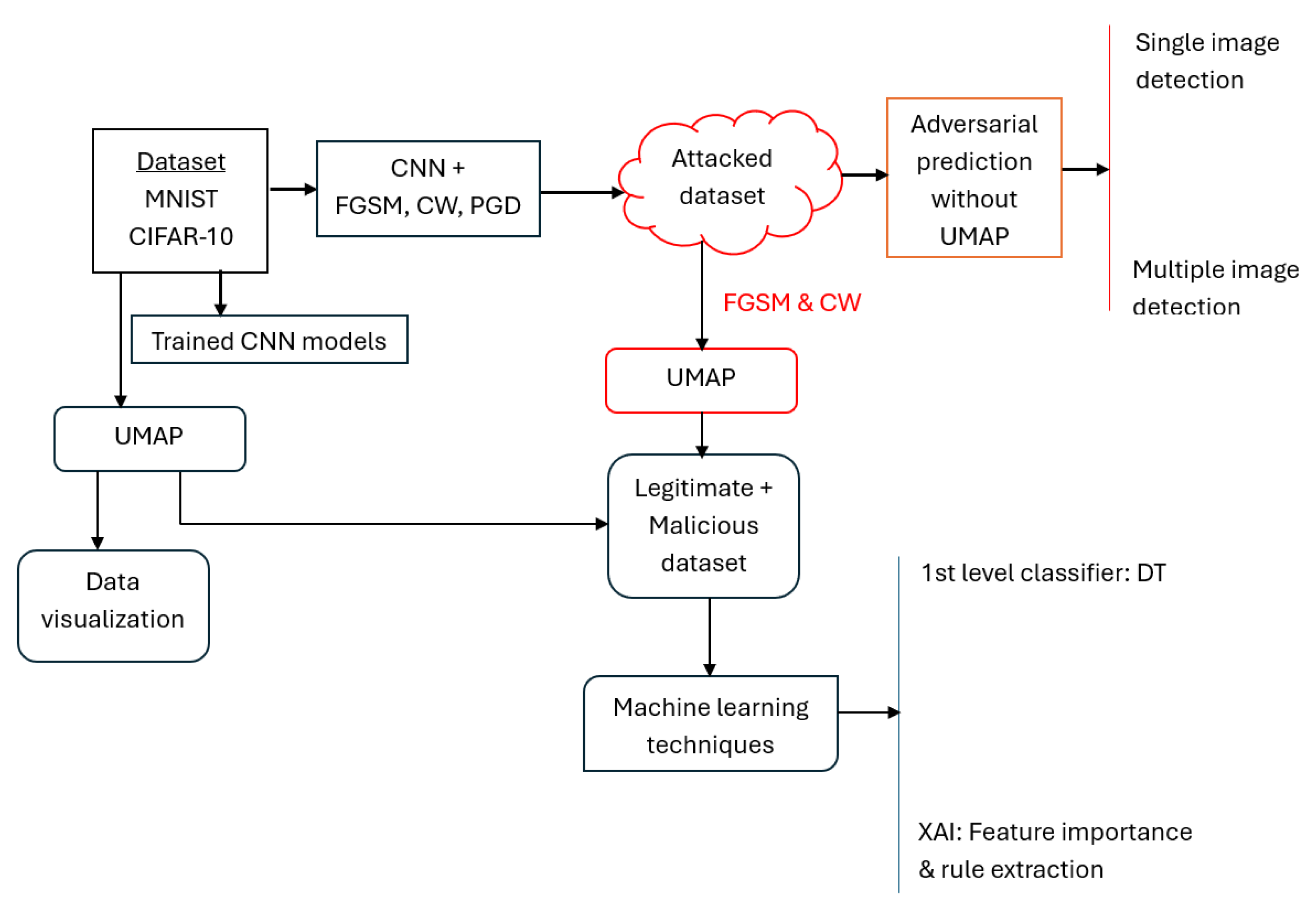
Figure 1.
Methodological workflow diagram outlining the sequential steps of CNN model training, adversarial attack generation, data visualization via UMAP, ligitimate and malicious data generation and analysis of generated UMAP data via XAI, and decision trees classifier.
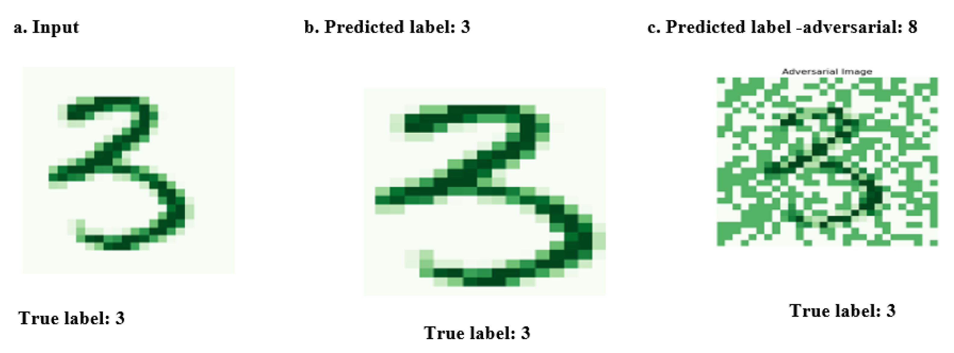
Figure 2.
The figure illustrates how adversarial attacks can lead to misclassification in the MNIST digit dataset, with some perturbations being visibly detectable.
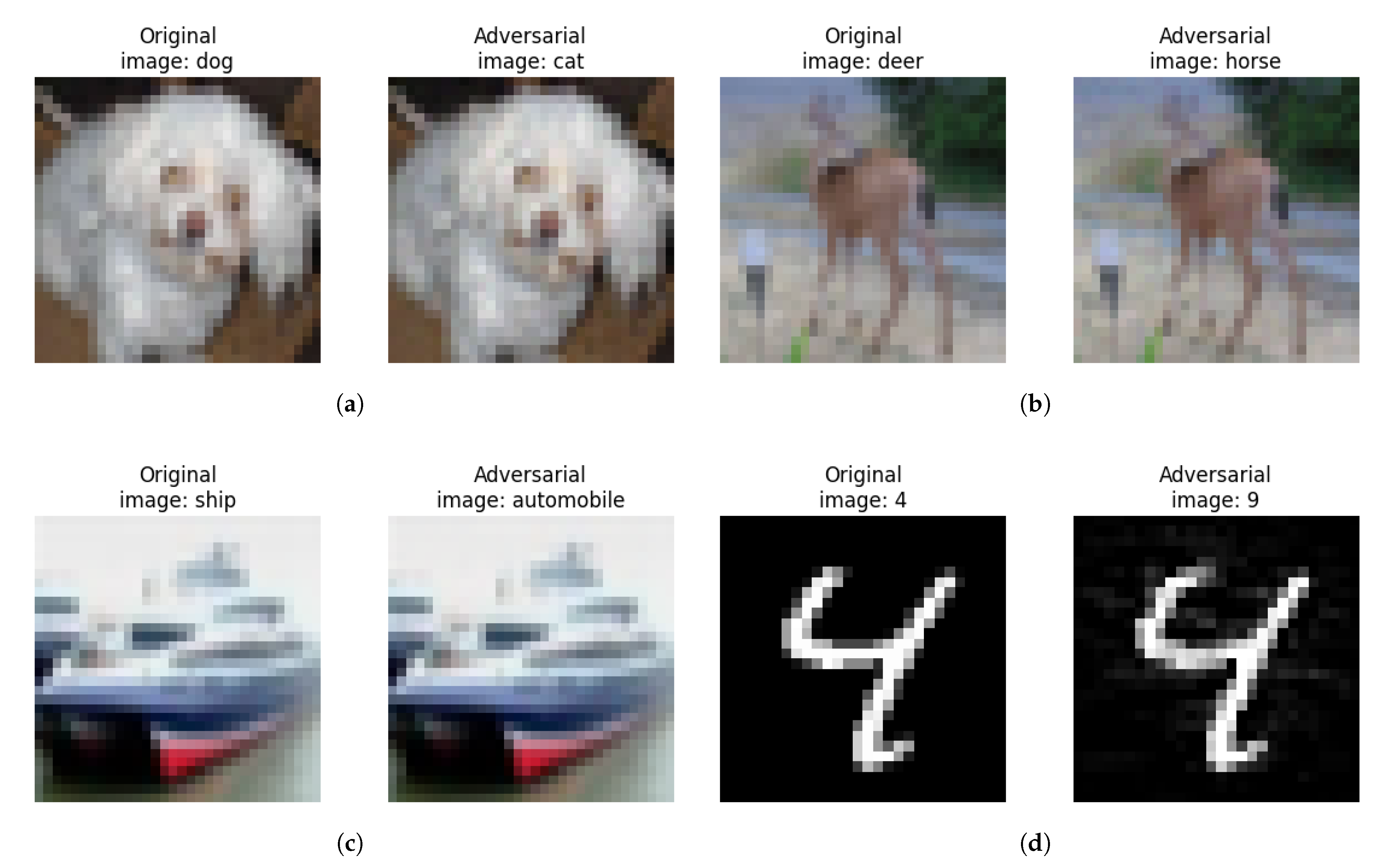
Figure 3.
Clean vs. adversarial examples from CIFAR-10 and MNIST demonstrate imperceptible perturbations generated by Carlini–Wagner, FGSM, and DeepFool attacks. Despite visual similarity to original inputs, all adversarial samples lead to model misclassification. (a) Clean vs. adversarial images of CIFAR10 dataset for Carlini–Wagner attack. (b) Clean versus adversarial images of CIFAR10 dataset for FGSM attack. (c) Clean vs. adversarial images of CIFAR10 dataset for DeepFool attack. (d) Clean versus adversarial images of MNIST dataset for DeepFool attack.
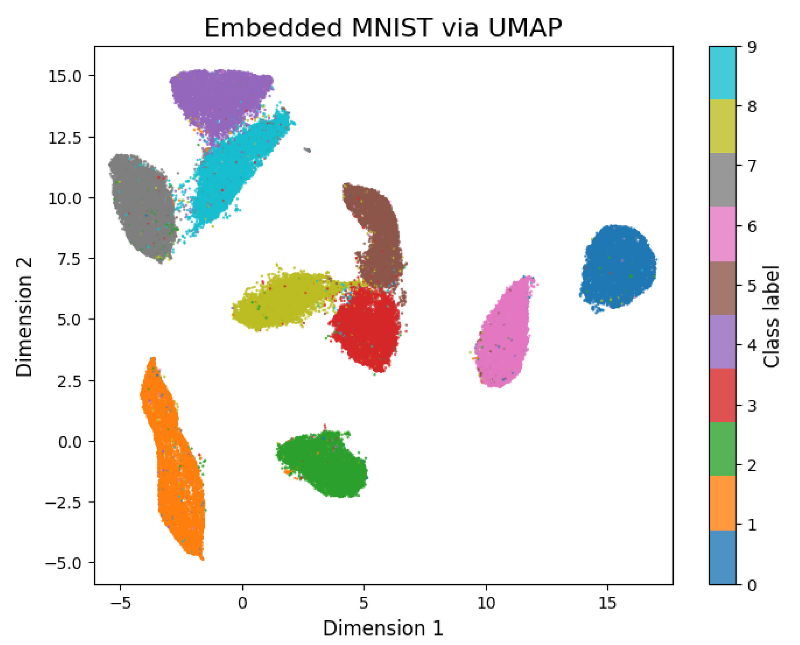
Figure 4.
UMAP 2D representations of the entire MNIST dataset. Digit classes form well-defined, identifiable clusters that are clearly separable from one another.
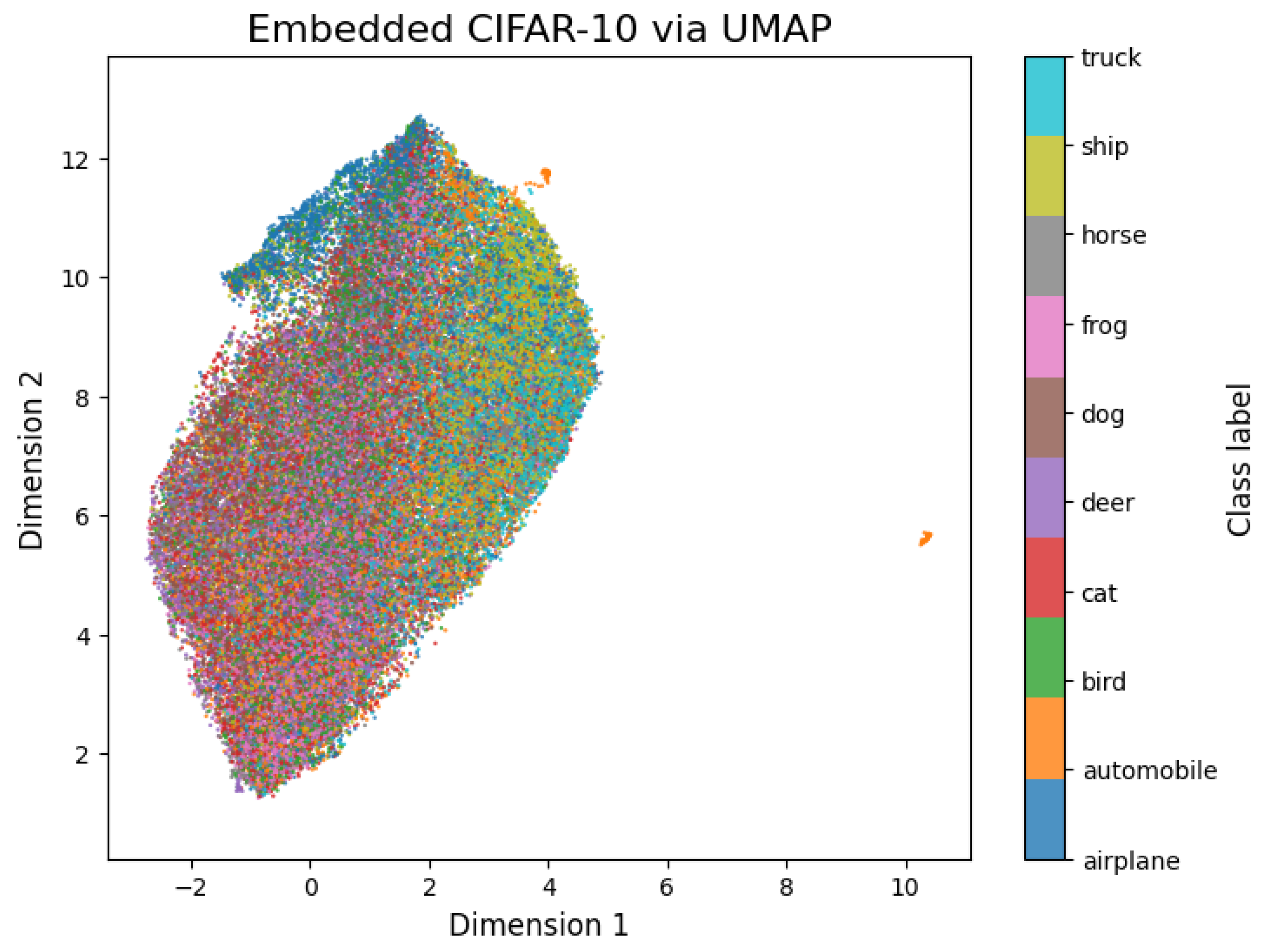
Figure 5.
UMAP 2D projection of the CIFAR-10 dataset. Different classes exhibit overlapping clusters, resulting in poor distinguishability and limited separability.
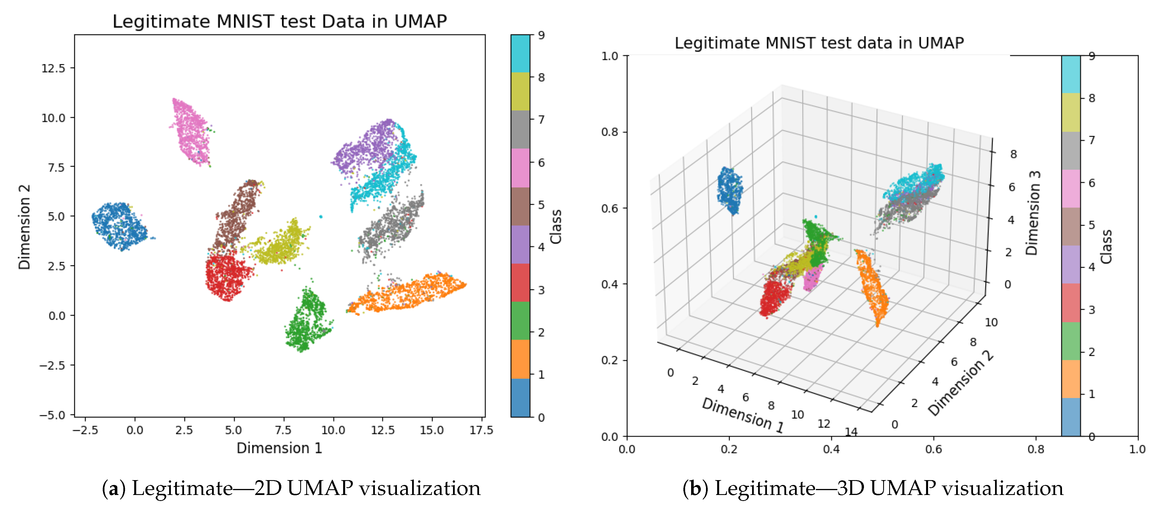
Figure 6.
UMAP projections of the legitimate MNIST test dataset in 2D (a) and 3D (b). These visualizations reveal the structure and clustering of digit classes in lower-dimensional space, enabling intuitive inspection of class separability and overlap.
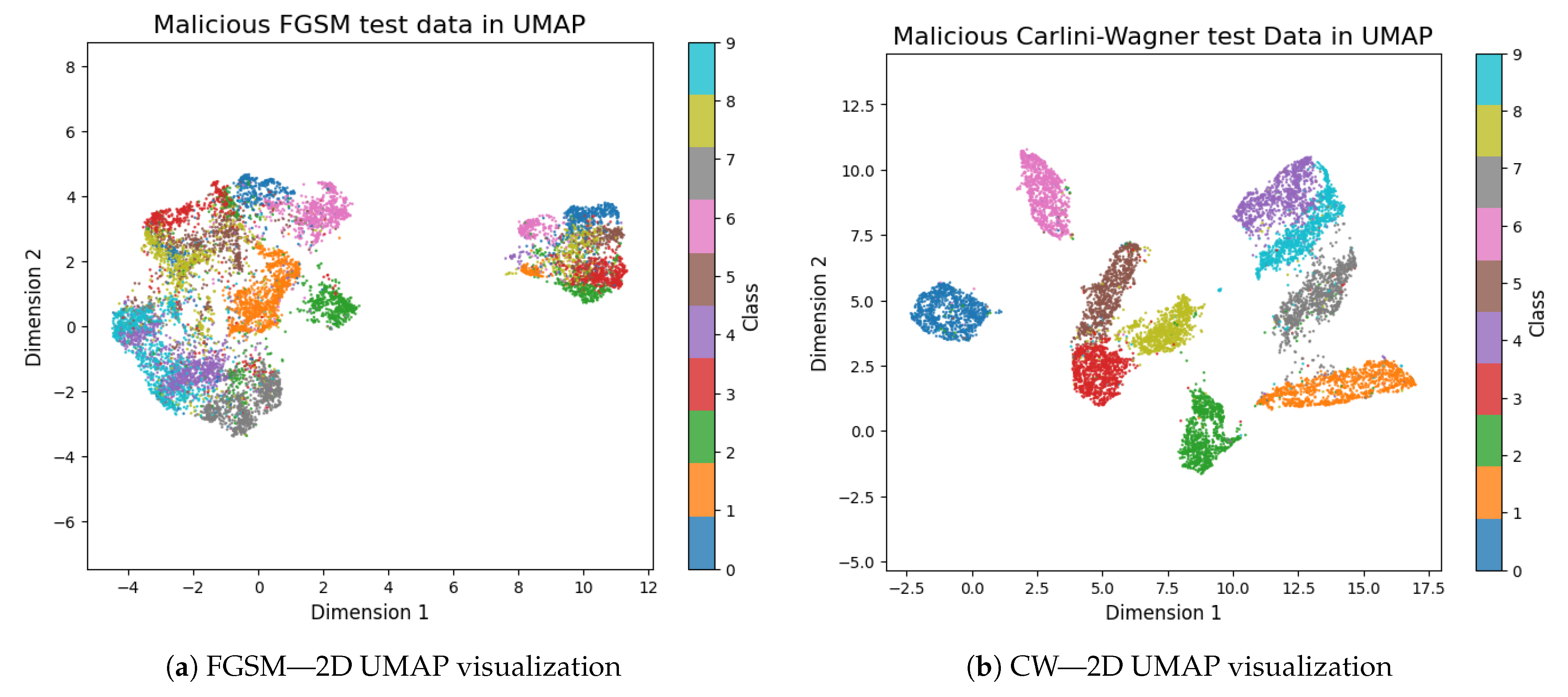
Figure 7.
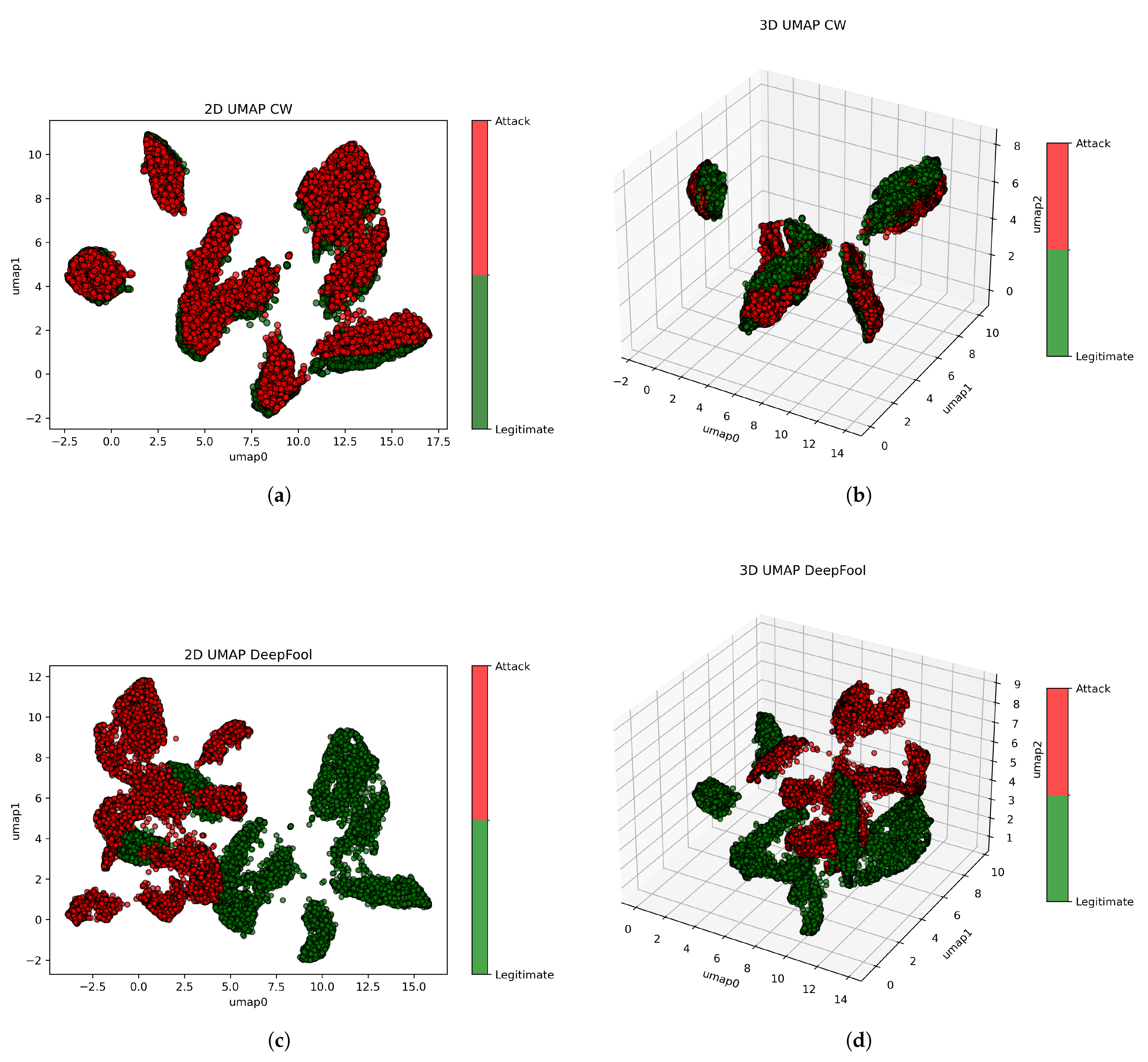
UMAP 2D projections of adversarial MNIST test samples: (a) FGSM attack and (b) CW attack. These visualizations illustrate how FGSM and CW attacks reduce class separability and increase overlap in the embedded space, compared to legitimate samples.
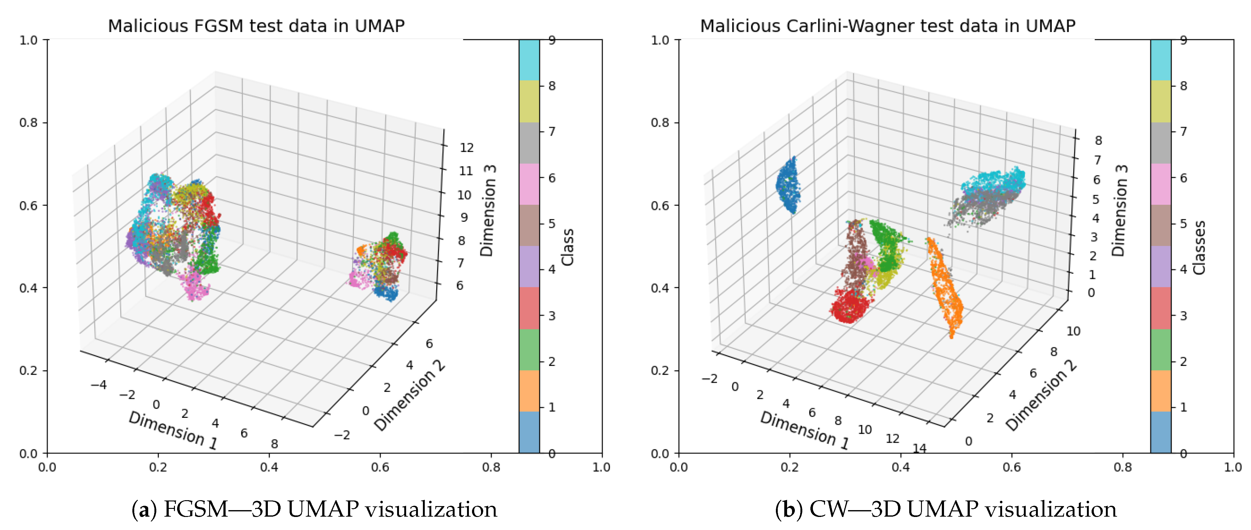
Figure 8.
UMAP 3D projections of adversarial MNIST test samples: (a) FGSM attack and (b) CW attack. The 3D visualizations reveal how adversarial perturbations reshape the spatial distribution of digit classes, leading to less distinct clustering and greater class overlap compared to legitimate data.
Figure 9.
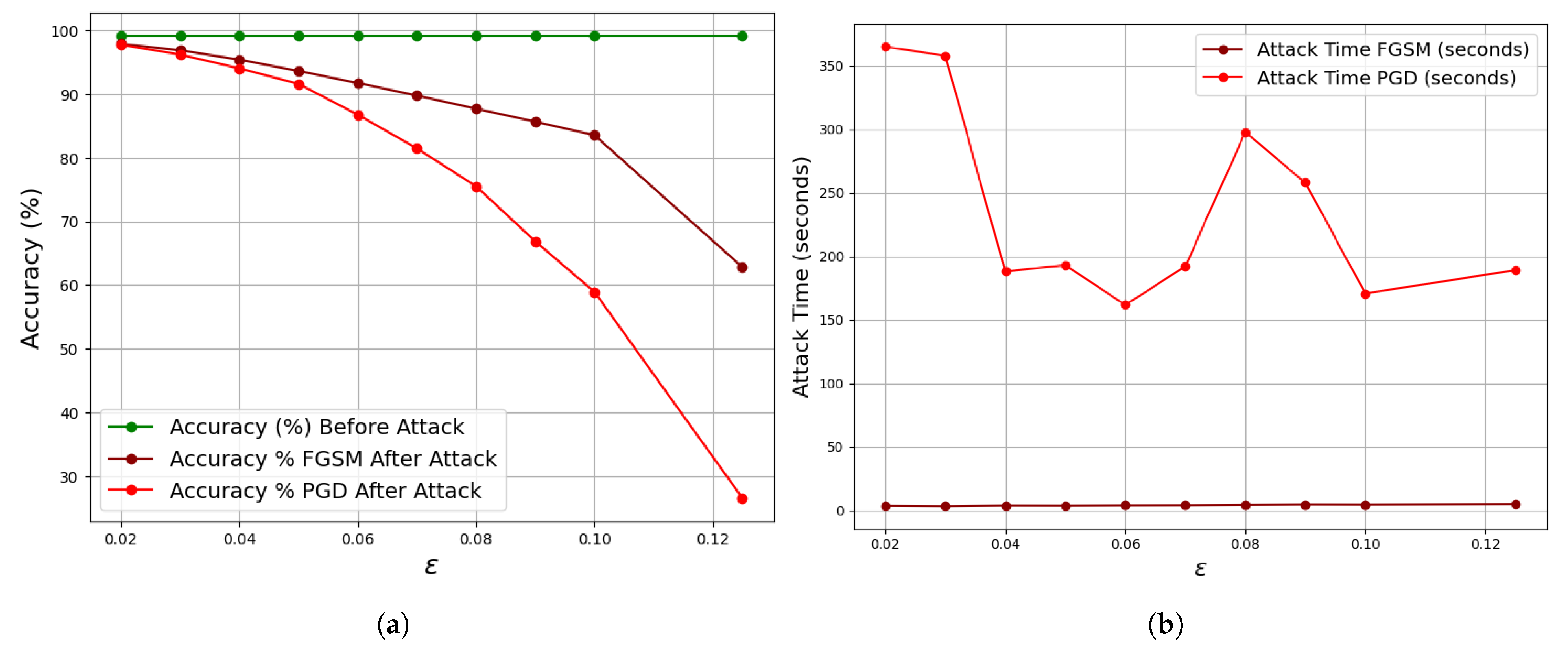
Accuracy and execution time for FGSM and PGD attacks at varying epsilon values on the MNIST dataset. The figure illustrates how increasing perturbation strength leads to a decline in model accuracy, highlighting increased susceptibility to adversarial attacks. PGD typically results in lower accuracy and greater computational cost compared to FGSM. (a) Accuracy vs. epsilon for FGSM and PGD attacks. (b) Computation time vs. epsilon for FGSM and PGD attacks.
Figure 10.
Comparison of accuracy and execution time for FGSM and PGD attacks on the CIFAR-10 dataset across varying epsilon values. As perturbation strength increases, classification accuracy declines, indicating higher model vulnerability. PGD consistently results in lower accuracy and longer execution times compared to FGSM. (a) Accuracy vs. epsilon for FGSM and PGD attacks. (b) Computation time vs. epsilon for FGSM and PGD attacks.
Figure 11.
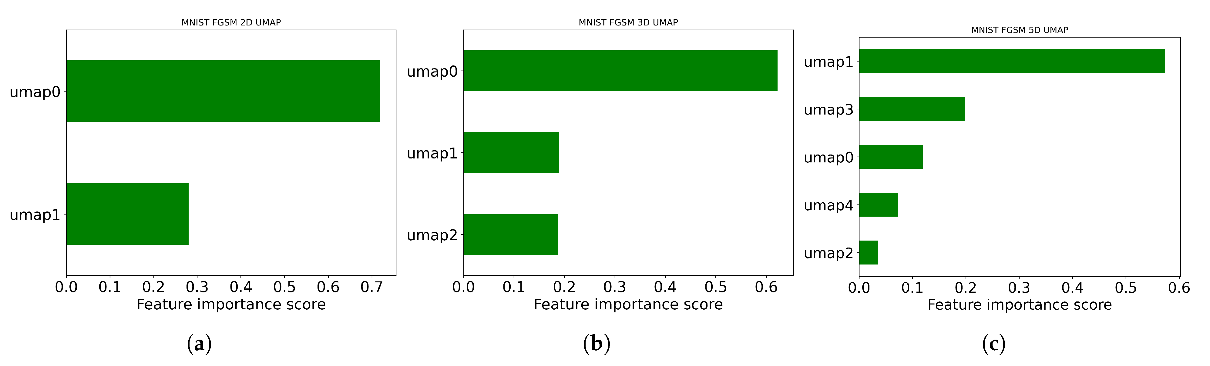
MNIST UMAP FGSM feature extraction. This figure shows the ranking order in 2D, 3D, and 5D, respectively, of the most important features of the MNIST dataset when FGSM attack is implemented. (a) Features—2D UMAP visualization. (b) Features—3D UMAP visualization. (c) Features—5D UMAP visualization.
Figure 12.
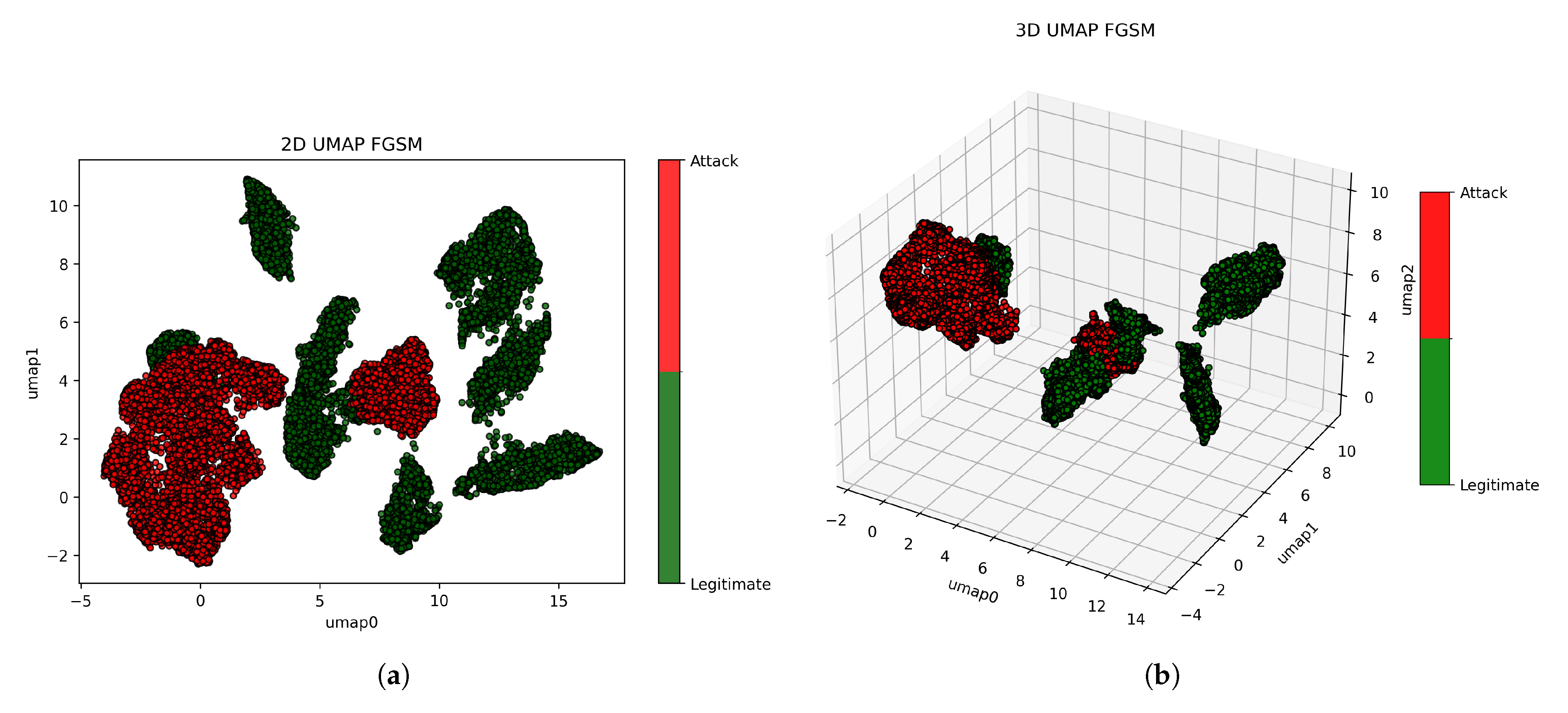
2D and 3D UMAP visualizations of MNIST under FGSM attack to physically observe the patterns and separability between legitimate (green) and adversarial (red) examples. (a) 2D UMAP plot of legitimate and adversarial examples. (b) 3D UMAP projection of legitimate and adversarial examples.
Table 1.
The table shows the success rates (%) of three adversarial attack techniques—FGSM, Carlini-Wagner, and DeepFool—on MNIST and CIFAR-10 datasets. Higher values indicate greater vulnerability of the models to adversarial perturbations.
| Dataset | FGSM | Carlini-Wagner | DeepFool |
|---|
| MNIST | 14.3 | 2.4 | 30.2 |
| CIFAR-10 | 69.3 | 99.5 | 94.3 |
Table 2.
Training parameters and accuracy for the MNIST and CIFAR-10 datasets.
| Parameters | MNIST Dataset | CIFAR-10 Dataset |
|---|
| Learning rate | 0.002 | 0.001 |
| Number of epochs | 50 | 20 |
| Batch size | 64 | 512 |
| Runtime type | CPU | T4GPU |
| Number of layers | 11 | 13 |
| Time to train the model | 47:33 min | 1:14 min |
| Accuracy of trained model | 99.2% | 74.87% |
Table 3.
Model accuracy and attack time comparison for MNIST: FGSM vs. PGD.
| Acc before Attack (%) | Time (s) FGSM | Acc After Attack FGSM (%) | Time (s) PGD | Acc After Attack PGD (%) |
|---|
| 0.02 | 99.20 | 3.7 | 97.88 | 365 | 97.74 |
| 0.03 | 99.20 | 3.4 | 96.87 | 358 | 96.19 |
| 0.04 | 99.20 | 3.9 | 95.39 | 188 | 94.03 |
| 0.05 | 99.20 | 3.8 | 93.62 | 193 | 91.60 |
| 0.06 | 99.20 | 4.0 | 91.73 | 162 | 86.77 |
| 0.07 | 99.20 | 4.1 | 89.76 | 192 | 81.47 |
| 0.08 | 99.20 | 4.4 | 87.69 | 298 | 75.52 |
| 0.09 | 99.20 | 4.7 | 85.65 | 258 | 66.88 |
| 0.10 | 99.20 | 4.6 | 83.55 | 171 | 58.94 |
| 0.125 | 99.20 | 5.0 | 62.81 | 189 | 26.56 |
Table 4.
Model accuracy and attack time comparison for CIFAR10: FGSM vs. PGD.
| Acc. Before Attack (%) | Time (s) FGSM | Acc. After Attack FGSM (%) | Time (s) PGD | Acc. After Attack PGD (%) |
|---|
| 0.001 | 75.68 | 4.1 | 74.66 | 340 | 74.64 |
| 0.002 | 75.68 | 4.5 | 72.79 | 367 | 72.75 |
| 0.005 | 75.68 | 111 | 66.19 | 344 | 65.76 |
| 0.006 | 75.68 | 6.0 | 63.07 | 384 | 62.44 |
| 0.007 | 75.68 | 7.6 | 60.03 | 369 | 59.62 |
| 0.01 | 75.68 | 7.3 | 51.42 | 338 | 50.64 |
| 0.02 | 75.68 | 6.9 | 32.28 | 347 | 30.67 |
| 0.03 | 75.68 | 10.8 | 27.38 | 561 | 21.15 |
| 0.04 | 75.68 | 6.2 | 24.09 | 343 | 16.79 |
| 0.1 | 75.68 | 6.4 | 15.06 | 463 | 12.16 |
Table 5.
Performance of FGSM adversarial attack detection on MNIST dataset without applying UMAP dimensionality reduction.
| Attack Success | Success Rate |
|---|
| 0.3 | 6727 | 0.6727 |
| 0.4 | 7546 | 0.7546 |
| 0.5 | 8007 | 0.8007 |
| 0.6 | 8339 | 0.8339 |
| 0.7 | 8515 | 0.8515 |
| 0.8 | 8662 | 0.8662 |
| 0.9 | 8743 | 0.8743 |
| 1.0 | 8796 | 0.8796 |
Table 6.
The table shows the results of the Carlini technique on the CIFAR-10 dataset across different dimensions for a comparison of UMAP and PCA. The FPR and FNR measure the error detection rate. All metrics are expressed in percentage.
| Dimension | UMAP | PCA |
|---|
| FPR | FNR | FPR | FNR |
|---|
| 2D | 29 | 44 | 22 | 82 |
| 3D | 45 | 33 | 78 | 26 |
| 5D | 1 | 2 | 16 | 87 |
| 10D | 0 | 0 | 15 | 87 |
Table 7.
Performance metrics for MNIST dataset: FGSM vs. Carlini–Wagner across dimensions 2D–10D with train–test split (TTS) and cross-validation score (CVS). The cross-validation score metrics validate the stability and generalizability detection of the model.
| Metrics | 2D | 3D | 5D | 10D |
|---|
| FGSM | CW | FGSM | CW | CW | CW | CW | CW |
|---|
| TTS | CVS | TTS | CVS | TTS | CVS | TTS | CVS | TTS | CVS | TTS | CVS |
|---|
| TPR | 97 | 96 | 97 | 98 | 97 | 97 | 84 | 72 | 93 | 91 | 100 | 100 |
| TNR | 90 | 90 | 15 | 13 | 98 | 98 | 50 | 67 | 80 | 81 | 100 | 100 |
| FPR | 10 | 10 | 85 | 87 | 2 | 2 | 50 | 33 | 20 | 19 | 00 | 00 |
| FNR | 3 | 4 | 3 | 2 | 3 | 3 | 16 | 28 | 7 | 8 | 00 | 00 |
| ACC | 93 | 93 | 56 | 56 | 98 | 97 | 67 | 69 | 86 | 87 | 100 | 100 |
| PPV | 90 | 91 | 53 | 53 | 98 | 98 | 62 | 69 | 82 | 83 | 100 | 100 |
| F1-Score | 93 | 93 | 69 | 69 | 98 | 97 | 72 | 70 | 87 | 87 | 100 | 100 |
Table 8.
Performance metrics for CIFAR-10: FGSM vs. Carlini–Wagner across dimensions 2D–10D with train–test split (TTS) and cross-validation score (CVS). The cross-validation score metrics validate the stability and generalizability detection of the model.
| Metrics | 2D | 3D | 5D | 10D |
|---|
| FGSM | CW | FGSM | CW | CW | CW | CW | CW |
|---|
| TTS | CVS | TTS | CVS | TTS | CVS | TTS | CVS | TTS | CVS | TTS | CVS |
|---|
| TPR | 99 | 97 | 56 | 67 | 100 | 100 | 67 | 52 | 98 | 99 | 100 | 100 |
| TNR | 93 | 94 | 71 | 58 | 100 | 100 | 55 | 70 | 99 | 99 | 100 | 100 |
| FPR | 7 | 6 | 29 | 43 | 0.00 | 0.00 | 45 | 29 | 1 | 1 | 0.00 | 0.00 |
| FNR | 1 | 1 | 44 | 33 | 0.00 | 0.00 | 33 | 48 | 2 | 1 | 0.00 | 0.00 |
| ACC | 96 | 96 | 64 | 62 | 100 | 100 | 61 | 61 | 98 | 99 | 100 | 100 |
| PPV | 93 | 94 | 66 | 62 | 100 | 100 | 60 | 66 | 99 | 99 | 100 | 100 |
| F1-Score | 96 | 96 | 60 | 64 | 100 | 100 | 63 | 56 | 98 | 99 | 100 | 100 |
Table 9.
Carlini–Wagner: Top 3 rules for MNIST 5D UMAP.
| Rule | Covering % | Error % |
|---|
| if umap4 and umap3 and umap0 and umap0 and umap2 and umap4 and umap3 then attack = True | 40.67 | 38.22 |
| if umap4 and umap3 and umap0 and umap0 and umap2 and umap4 and umap0 then attack = True | 9.45 | 1.29 |
| if umap4 and umap3 and umap2 and umap4 and umap1 and umap2 and umap0 then attack = False | 9.15 | 7.89 |
Table 10.
Carlini–Wagner: Rules for MNIST 10D UMAP.
| Rule | Covering % | Error % |
|---|
| if umap9 then attack = True | 100 | 0 |
| if umap9 then attack = False | 100 | 0 |
Table 11.
FGSM: Rules for MNIST 10D UMAP.
| Rule | Covering % | Error % |
|---|
| if umap8 then attack = True | 100 | 0 |
| if umap8 then attack = False | 100 | 0 |
Table 12.
Detection performance metrics for the DeepFool attack on the MNIST dataset using a decision tree classifier across UMAP dimensions (2D–10D). Metrics are reported using train–test split (TTS) and cross-validation score (CVS) and are all reported in percentages. Attack parameters: , , , , .
| Metrics | 2D | 3D | 5D | 10D |
|---|
| TTS | CVS | TTS | CVS | TTS | CVS | TTS | CVS |
| TPR | 97.7 | 99.9 | 99.6 | 91.0 | 99.9 | 99.5 | 100 | 100 |
| TNR | 92.4 | 77.6 | 98.0 | 85.6 | 100 | 99.5 | 100 | 100 |
| FPR | 7.61 | 22.3 | 2.03 | 14.4 | 0.00 | 0.6 | 0.00 | 0.00 |
| FNR | 2.35 | 0.06 | 0.4 | 9.0 | 0.1 | 0.5 | 0.00 | 0.00 |
| ACC | 95.0 | 88.8 | 98.8 | 88.3 | 99.9 | 99.5 | 100 | 100 |
| PPV | 93.0 | 81.7 | 98.0 | 86.3 | 100 | 99.5 | 100 | 100 |
| F1-Score | 95.1 | 89.9 | 98.8 | 88.6 | 99.9 | 99.5 | 100 | 100 |
Table 13.
DeepFool: Rules for MNIST 10D UMAP.
| Rule | Covering % | Error % |
|---|
| if umap6 then attack = True | 100 | 0 |
| if umap6 then attack = False | 100 | 0 |


