Explainable Machine Learning Model for Source Type Identification of Mine Inrush Water

Abstract

The prevention and control of mine inrush water has always been a major challenge for safety. By identifying the type of water source and analyzing the real-time changes in water composition, sudden water inrush accidents can be monitored in a timely manner to avoid major accidents. This paper proposes a novel explainable machine learning model for source type identification of mine inrush water. The paper expands the original monitoring system into the XinJi No.2 Mine in Huainan Mining Area. Based on the online water composition data, using the Spearman coefficient formula, it analyzes the water chemical characteristics of different aquifers to extract key discriminant factors. Then, the Conv1D-GRU model was built to deeply connect factors for precise water source identification. The experimental results show an accuracy rate of 85.37%. In addition, focused on the interpretability, the experiment quantified the impact of different features on the model using SHAP (Shapley Additive Explanations). It provides new reference for the source type identification of mine inrush water in mine disaster prevention and control.

1. Introduction

As coal mining advances in depth, the geological conditions of mines are becoming increasingly complex. Several factors such as the development of water-conducting fissures and multi-layer mining voids have exacerbated the water hazard problem faced by the safe mining of coal. Generally, due to the influence of geological structures and water migration, the hydrochemical characteristics of water bodies in different aquifers in mines are distinct. Various types of water bodies may cause inrush water in mines, but their degrees of harm and the methods for prevention and control differ. Quickly and accurately identifying the type of water source of the inrush is crucial for the prevention and control of inrush water disasters.

Source type identification of mine inrush water is a major application of technology in mine water prevention and control. By using microscopic chemical characteristics such as ion content to research the differences and connections among different aquifers, it is possible to determine the hydrogeological characteristics and recharge sources of aquifers that have a significant impact on sudden water inrush in mines. The microscopic chemical characteristics of water can be determined using methods including the representative ion method, isotope method, trace element method, water temperature and water level method, etc. [1].

The representative ion method usually selects seven major ions, including ${\mathrm{K}}^{+}$, $\mathrm{N}{\mathrm{a}}^{+}$, $\mathrm{C}{\mathrm{a}}^{2+}$, $\mathrm{M}{\mathrm{g}}^{2+}$, $\mathrm{C}{\mathrm{l}}^{-}$, $\mathrm{S}{\mathrm{O}}_4^{2-}$, and ${\mathrm{HCO}}_3^{-}$, to detect the differences in the content of inorganic substances in water bodies. Further, piper diagrams, ion box diagrams, etc., are often used for statistical analysis of each aquifer, and then statistical learning and other mathematical methods are used for source type identification [2]. Isotopes are relatively stable and do not interact with other components of the water body, thus providing good tracing effects for the water body. Therefore, they are widely applied in studies on the origin of groundwater, the development laws of aquifers, etc. [3]. The trace elements that can trace the water chemical characteristics of the aquifer provide supplementary evidence for constructing the water inrush discrimination model [4]. The water temperature method generally has good discriminant effects for different aquifers with significant stratigraphic differences [5].

The above methods for extracting water characteristics currently rely on chemical measurements, which have a lengthy test process and cause secondary pollution of the water body through the mixing of chemical reagents. Professional instruments such as chromatography–mass spectrometers are expensive. Apart from a few professional testing laboratories, most coal mines lack the capability for such detection. Additionally, the equipment operation is complex, requiring clean water samples without the interference of dissolved organic substances and suspended solids. The equipment is also bulky and not suitable for on-site carrying and installation, making it difficult to meet the real-time monitoring requirements of mine water gushing. Consequently, the optimal opportunity to manage water outburst incidents is often missed, resulting in frequent major accidents [6,7,8].

The research project on “Real-time Monitoring and Early Warning Technology for Major Mine Water Inrush Disasters” conducted by China University of Mining and Technology within the “Twelfth Five-Year National Science and Technology Support Program” designed an online discrimination monitoring system for the source types of mine water inrush based on the Internet of Things. The monitoring nodes consist of conductivity sensors, pH sensors, $\mathrm{C}{\mathrm{a}}^{2+}$, $\mathrm{N}{\mathrm{a}}^{+}$, ${\mathrm{HCO}}_3^{-}$, and $\mathrm{C}{\mathrm{l}}^{-}$ concentration sensors, and fluorescence spectroscopy sensors. These sensors collect data and transmit information in real time and have a short test process. By integrating physical and chemical laws such as geophysics, geochemistry, and rock mechanics, conducting information fusion analysis on aspects such as water inrush hazard sources, fracture of aquifers, and early water inrush, significant progress has been made in effectively preventing and controlling major mine water inrush disasters [9].

On the other hand, with the continuous progress of artificial intelligence, researchers are constantly looking for new methods to improve the real-time monitoring and early warning of mine inrush water. In the aspect of diagnosis model, over the past few years, scientists have been trying to apply various sophisticated mathematical and complex system theories, including expert system, inverse modeling, pattern recognition, and machine learning, to predict inrush water risk assessment from the perspectives of identification of water sources [9,10,11,12,13]. At the same time, data-driven intelligent diagnosis models have become an important direction to break through the bottleneck of traditional methods. Among them, the DL (deep learning) model provides new ideas for efficient and accurate identification of inrush water sources by virtue of its powerful nonlinear mapping ability, automatic feature extraction, and adaptability to high-dimensional complex data [14,15,16,17].

The DL model can automatically learn the most representative features from a large amount of data and output highly accurate prediction results. However, as the complexity of the DL model increases, its internal operating mechanism gradually becomes an incomprehensible “black box” with no basis for decision-making. To solve the “black box” problem of the DL model, researchers have proposed explainable ML (explainable machine learning) [18,19]. This approach requires the model not only to provide the results but also to explain the reasons behind them. When constructing the model, both the prediction accuracy and the model explainability are considered, with an optimal balance between the two being sought.

This work put forward an explainable machine learning model for source type identification of mine inrush water. Expanding upon China University of Mining and Technology’s “Twelfth Five-Year Plan” monitoring system, the study extends the original scope to the Huainan Mining Area’s XinJi No.2 Mine. Key discriminative hydrochemical factors are extracted through Spearman coefficient analysis of aquifer characteristics.

Conv1d (convolutional layer 1D convolution) enhances its ability to extract multidimensional features by increasing the number of channels, while a GRU (gated recurrent unit) network captures the sequential dependencies in the data and enhances feature representation. Through interpretable experiments, the Conv1d-GRU network model quantifies the impact of aquifer characteristics on the identification of water source types.

The main contributions are as follows:

• A novel Conv1d-GRU network is developed for accurate source type identification of mine inrush water.
• The Spearman coefficient analysis and interpretability experiments quantify the impact of key features on model performance.

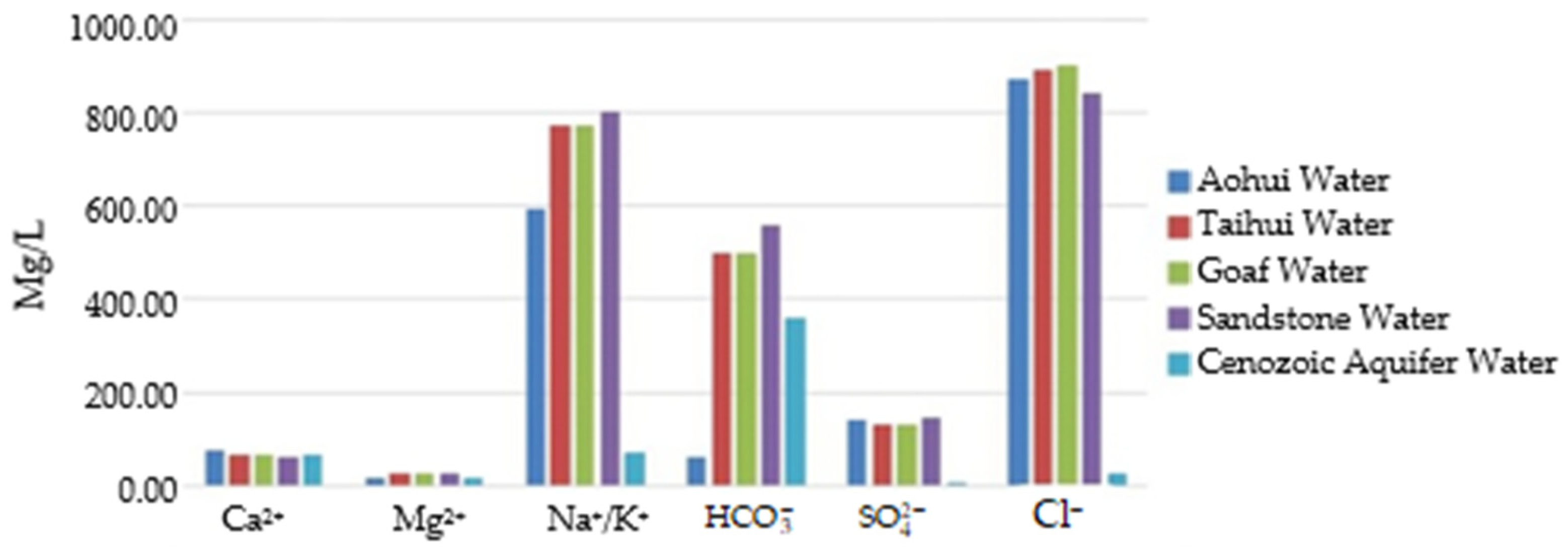
2. Hydrochemical Characteristics of Hydrogeological Mines

The paper focuses on Xinji No.1 Mine and Xinji No.2 Mine in Huainan Mining Area. Huainan Mining Area is located in the south of the North China platform, and its geological structure belongs to the Qinling zonal belt east extension. Huainan coalfield is composed of Guzhen changfeng normal fault in the east, Shouxian Laorencang normal fault in the south, Kouzi Nanzhao normal fault in the west, and Shangtang Minglongshan reverse fault in the north. It roughly forms the water control boundary in the east, south, west, and north, on all four sides, and basically becomes a separate hydrogeological unit. The entire Huainan coalfield is located on both sides of the middle reaches of the Huaihe River. To the east and southeast of the coalfield are mountains with exposed bedrock, and to the north and northwest is the Huang–Huai alluvial plain.

The Mining Field is divided into five aquifer groups from top to bottom: Cenozoic aquifer water (Cenozoic unconsolidated aquifer water), sandstone water (Permian sandstone fracture water), goaf water, Taihui water (Taiyuan Formation limestone karst fracture water), and Aohui water (Ordovician carbonate karst fracture water).

In accordance with the above classification, this paper collected water sources as a sample library, and obtained five types of samples in batches, including sandstone water, goaf water, Taihui water, Aohui water, and Cenozoic aquifer water, with 40 samples in each category, totaling 201 samples. The samples were placed in polypropylene vials that had been washed with 10% HCl and distilled water, and the fluorescence spectrum, pH, TDS (total dissolved solids), and water chemical characteristic ions were determined promptly.

Additionally, Figure 1 depicts a comparison map of ion concentrations, derived from the average values of each ion concentration in each aquifer. The ion concentration in the Cenozoic aquifer water is lower than that of the other water sources, and the concentration of ${\mathrm{HCO}}_3^{-}$ ions is higher. Except for the Cenozoic aquifer water, the ion concentration levels of other aquifers are essentially the same. In general, the ion content of sandstone water is relatively high, but the difference is not markedly distinct compared to other aquifers. The concentrations of $\mathrm{N}{\mathrm{a}}^{+}/{\mathrm{K}}^{+}$ ions, ${\mathrm{HCO}}_3^{-}$ ions, and $\mathrm{C}{\mathrm{l}}^{-}$ ions in the five water samples were relatively high. Except for bicarbonate ions in Neozoic water and ash water, they all reached 550 mg/L, 350 mg/L, and 600 mg/L, and the lowest average concentration of magnesium ions was less than 50 mg/L. Except for Neozoic water and ${\mathrm{HCO}}_3^{-}$ ions in Aohui water, all concentrations reached 550 mg/L, 350 mg/L, and 600 mg/L, respectively, and the average concentration of $\mathrm{M}{\mathrm{g}}^{2+}$ ions was the lowest, at less than 50 mg/L.

As shown in Figure 1, the six ions concentration are numbered as X₁, X₂, …, X₆. In conjunction with pH, TDS, alkalinity and hardness features. A feature set was constructed to form a machine learning database. For simplicity, Aohui water, sandstone water, goaf water, Taihui water, and Cenozoic aquifer water are labeled as Y₁, Y₂, Y₃, Y₄, and Y₅, respectively, as shown in

Table 1. Feature/label name.

Features	Name
Ca2+	X1
Mg2+	X2
Na+/K+	X3
HCO3−	X4
SO42−	X5
Cl−	X6
pH	X7
TDS	X8
Alkalinity	X9
Hardness	X10
Aohui Water	Y1
Sandstone Water	Y2
Goaf Water	Y3
Taihui Water	Y4
Cenozoic Aquifer Water	Y5

.

3. Methodology

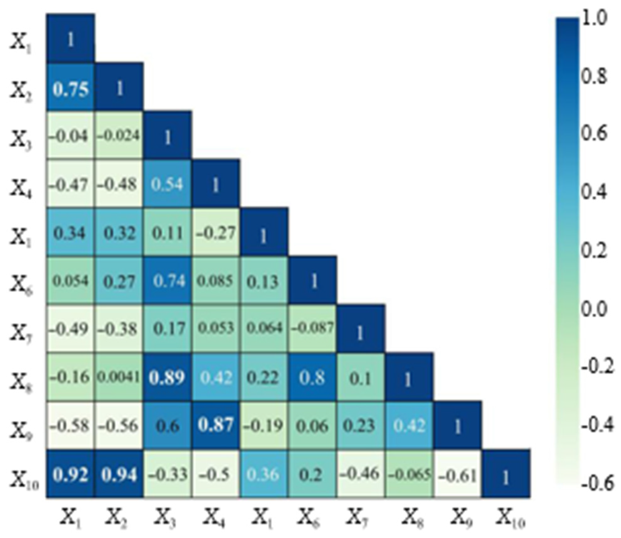
3.1. Correlation Analysis

The Spearman rank correlation coefficient is a statistical method used to evaluate the monotonic relationship between two variables, which is adaptable for processing nonlinear or non-normal data. Different from the Pearson correlation coefficient, the Spearman coefficient measures the correlation by comparing the rankings of the variables. Therefore, it has better applicability for dealing with outliers or skewed data.

(1) Data sorting: First, the input features are standardized. Next, the observed values are arranged in ascending order and assigned a corresponding rank. When values are identical, they are assigned the same rank.

(2) Calculate ranking difference: For each pair of observations (X, X′), calculate their ranking difference.

(3) Square ranking difference: Square each ranking difference d_i to obtain d_i².

(4) Summation: Add up all the differences between the ranks after squaring them to obtain the total sum of di².

(5) Correlation coefficient calculation: Obtain the correlation coefficient value based on the following formula:

$$p(X,X^{\prime })={\displaystyle \frac{1-(6{\displaystyle \sum {(R(x_i)- R(x_i^{\prime }))}^2})}{n(n^2-1)}}$$

(1)

where p (X, X′) represents the Spearman correlation coefficient of two different features X and X′. R(x_i) − R(x′_i) = d_i, where R(x_i) and R(x′_i), respectively, represent the ranking values of x_i and x′_i; n is the total sample size. The value range of the Spearman correlation coefficient is from −1 to 1, where −1 indicates a completely negative correlation, 1 indicates a completely positive correlation, and 0 indicates no monotonic relationship. Based on the water inrush source database, positive and negative correlations between the features were obtained using the Spearman correlation coefficient method. The experimental results are shown in Figure 2.

As shown in Figure 2, the correlation coefficients between X₁ and X₁₀, as well as between X₂ and X₁₀, are 0.92 and 0.94, respectively, indicating an extremely strong correlation between X₁₀ and X₁ and X₂. Considering that the correlation coefficient between X₁ and X₂ is 0.75, it shows that there is a strong positive correlation among the three features. Additionally, the correlation coefficients between X₃ and X₈, as well as between X₄ and X₉, are 0.89 and 0.87, respectively, indicating a very strong positive correlation between X₃ and X₈, and between X₄ and X₉. Therefore, in the subsequent research, it is necessary to consider eliminating the strongly correlated features and verifying whether the database is redundant. Based on the above experimental results, this paper considers eliminating the features X₁, X₃, and X₄.

3.2. LSTM Network

The LSTM (long-short time memory) network effectively captures and remembers long-term dependencies via its gating mechanism. The three key control modules are the input gate ${\mathit{i}}_{\mathit{t}}$, the output gate ${\mathit{o}}_{\mathit{t}}^{\prime }$, and the forget gate ${\mathit{f}}_{\mathit{t}}$. The input gate decides which input information should be added to the current state, the output gate determines which information should be output from the current state ${\mathit{c}}_t$, and the forget gate’s core function is to select the information to be discarded when updating the cell state. The control principle of the model is illustrated in Equations (2)–(6).

$${\mathit{f}}_{\mathit{t}}=\mathrm{sigmoid} ({\mathit{W}}_{\mathit{f}}\ast [{\mathit{h}}_{\mathit{t}-1,}{\mathit{x}}_{\mathit{t}}+{\mathit{b}}_{\mathit{f}}])$$

(2)

$${\mathit{i}}_{\mathit{t}}=\mathrm{sigmoid} ({\mathit{W}}_i\ast [{\mathit{h}}_{\mathit{t}-1,}{\mathit{x}}_{\mathit{t}}+{\mathit{b}}_i])$$

(3)

$${\mathit{c}}_{\mathit{t}}={\mathit{i}}_{\mathit{t}} \ast \tanh ({\mathit{W}}_c\ast [{\mathit{h}}_{\mathit{t}-1,}{\mathit{x}}_{\mathit{t}}+{\mathit{b}}_c])+{\mathit{f}}_{\mathit{t}}\ast {\mathit{c}}_{\mathit{t}-1}$$

(4)

$${\mathit{o}}_{\mathit{t}}^{\prime }=\mathrm{sigmoid} ({\mathit{W}}_o\ast [{\mathit{h}}_{\mathit{t}-1,}{\mathit{x}}_{\mathit{t}}+{\mathit{b}}_o])$$

(5)

$${\mathit{h}}_{\mathit{t}}={\mathit{o}}_{\mathit{t}}^{\prime } \ast \tanh ({\mathit{c}}_{\mathit{t}})$$

(6)

where W_f and bf are the weight coefficient matrix and bias vector of the forgetting gate, respectively. h_t−1 represents the output of the previous unit at the previous time step, x_t represents the input of the current unit, W_i and W_c are the weight coefficient matrices in the input gate after the activation function processing, b_i and b_c are the bias vectors of the input gate, W_o represents the weight coefficient matrix of the output gate, and b_o is the bias vector of the output gate, with $o_t^{\prime }$ representing the output at time step t.

3.3. GRU Network

The GRU network modifies the gating mechanism of LSTM. The reset gate ${\mathit{r}}_{\mathit{t}}$ controls how much the current input updates the current hidden state, while the update gate ${\mathit{z}}_{\mathit{t}}$ determines how much information to pass to the subsequent state. The candidate state gate ${\mathit{h}}_{\mathit{t}}$ combines the current input information with the filtered historical information. A gating mechanism is used to control the flow of information, and the candidate states, in conjunction with the update gate, determine the information that is ultimately passed to the next time step. Equations (7)–(10) describe this calculation process.

$${\mathit{r}}_{\mathit{t}}=\mathit{\sigma } ({\mathit{W}}_r{x}_t^{\prime }+{\mathit{U}}_r{\mathit{h}}_{\mathit{t}-1}+{\mathit{b}}_{\mathit{r}})$$

(7)

$${\mathit{z}}_{\mathit{t}}=\mathit{\sigma } ({\mathit{W}}_z{x}_t^{\prime }+{\mathit{U}}_z{\mathit{h}}_{\mathit{t}-1}+{\mathit{b}}_z)$$

(8)

$${\tilde{\mathit{h}}}_{\mathit{t}}=\tanh ({\mathit{W}}_h{x}_t^{\prime }+{\mathit{U}}_h({\mathit{r}}_{\mathit{t}}\odot {\mathit{h}}_{\mathit{t}-1})+{\mathit{b}}_h)$$

(9)

$${\mathit{h}}_{\mathit{t}}={\mathit{z}}_{\mathit{t}}\odot {\mathit{h}}_{\mathit{t}-1}+(1-{\mathit{z}}_{\mathit{t}})\odot {\tilde{\mathit{h}}}_{\mathit{t}}$$

(10)

where σ and tanh represent sigmoid and tanh activation function. W_z, W_r, and W_h are the weight matrices of input to the update gate, reset gate, and candidate output. b_k, b_z, b_r, and b_h are the bias vectors of the update gate, reset gate, and candidate output. U_z, U_r, and U_h are the weight matrices of the hide states of the reset gates, update gates, and candidate states; h_t−1 is the hidden state of the previous time step; ${\mathit{x}}_{\mathit{t}}^{\prime }$ is the input at the current time; and $\odot$ is matrix multiplication.

3.4. Conv1d Network

CNN (convolutional neural network) employs a one-dimensional convolution kernel to process water data. By utilizing local perception, spatial arrangement, and parameter sharing, it can extract local correlation features from water data more rapidly and precisely, thereby further optimizing the effect of feature representation. The calculation process for the number of features is illustrated in Equation (11).

$${\mathit{F}}_{\mathit{o}\mathit{u}\mathit{t}}={\displaystyle \frac{{\mathit{F}}_{in}+2\times Padding-k\_s}{Stride}}+1$$

(11)

where F_in and F_out are the number of input and output features; Padding represents filling on both sides of the input data; k_s is used to define the size of the convolution kernel; and Stride is used to determine the step size of the convolution operation.

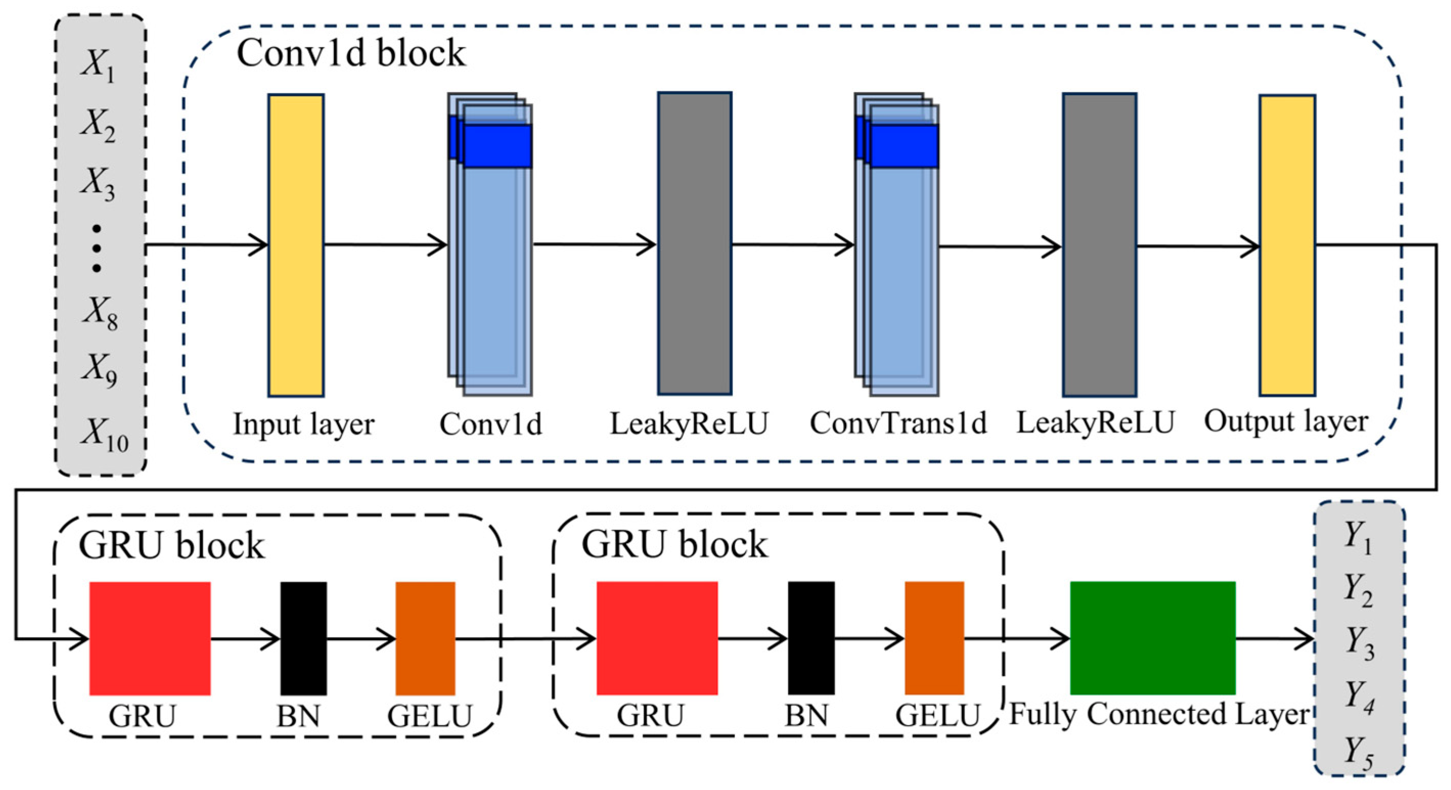
3.5. Conv1d-GRU Network

The paper proposes a model combining GRU and the Conv1d structure for mine inrush water source type identification. As shown in Figure 3, the overall network consists of a one-dimensional convolutional feature extraction module, a gated recurrent unit block, and a fully connected output layer, which is used to deal with multidimensional sequence classification tasks.

Firstly, a convolution kernel of size 3 is used to extract the local features of the original input data with a step size of 1, and the convolution results are obtained with the number of output channels set to 16. Then, in the LeakyReLU activation function, the slope coefficient of the negative half axis is set to 0.01 for nonlinear transformation, which enhances the nonlinear expression ability of the model and avoids the problem of neuron deactivation. Then, a one-dimensional transposed convolution (ConvTrans1d) operation is connected. The kernel size is set to 3, the stride is 1, and the output channel number is 7. This operation aims to perform upsampling reconstruction on the feature maps extracted by the convolution in the channel dimension, enhancing their feature expression ability. Through the learnable transposed convolution kernel, the model can more effectively restore the important detailed features lost during the previous convolution process, providing a more abundant input for the subsequent GRU module. The LeakyReLU activation function is used to strengthen the modeling ability of the model for complex patterns.

Then, two GRU modules are concatenated. Each GRU module contains a GRU layer with 18 hidden units, the batch normalization layer is connected to stabilize the intermediate feature distribution, and the GELU activation function is combined to enhance the nonlinear fitting ability. The equation expression is as follows:

$$\mathrm{GELU}(x)=0.5x\left(1+\tanh \left[\sqrt{{\displaystyle \frac{2}{\pi }}}\left(x+0.044715x^3\right)\right]\right)$$

(12)

Finally, the features from the last hidden state of the second GRU layer integrate into the fully connected layer to provide the classification result. Through the above structure design, the model can fully integrate the ability of local feature extraction and long sequence modeling and improve the classification accuracy while ensuring computational efficiency.

4. Experiments and Results

4.1. Experiment Setup

Models were built using PyTorch2.6.0 and Python3.7. The model uses an Adam optimizer with a learning rate of 0.0005, batch size of 8, and 500 training rounds. To ensure comparative experiments, data were divided into 80% training and 20% testing for all models. This study employed stratified sampling to ensure that the label distribution of the training/validation sets was consistent with that of the original data. To prevent overfitting of the model, the threshold for the performance of the validation set was set at 85%, at which point the training will automatically stop. The specific parameters of the Conv1d-GRU model are shown in

Table 2. Conv1d-GRU model parameters.

Names	Input Shape	Output Shape
CNN Input	(8, 10)	(8, 7, 1)
Conv1d-1	(8, 7, 1)	(8, 7, 1)
Conv1d-2	(8, 7, 1)	(8, 7, 16)
Conv1d-3	(8, 7, 16)	(8, 7, 16)
CNN Output	(8, 7, 1)	(8, 7)
GRU	(8, 7)	(8, 18)
GRU	(8, 18)	(8, 18)
Output	(8, 18)	(8, 5)

.

To evaluate the model’s training process and its generalization capabilities, this paper documents the classification accuracy of both the training and validation sets for each iteration throughout the training phase. It then plots the accuracy trends over the number of iterations, as depicted in Figure 4. Observations reveal that the model’s accuracy rises sharply in the initial stages of training and subsequently levels off. The validation set’s accuracy meets the predetermined threshold (85%) by the 300th iteration, satisfying the early stopping criterion. The overall trend indicates that the accuracies of both the training and validation sets evolve in tandem, with no significant signs of overfitting. This suggests that the proposed model exhibits strong convergence and generalization capabilities for this task.

Further, the GRU and LSTM networks are configured with identical parameters, as outlined in

Table 3. GRU and LSTM model parameters.

Names	Layers	Output Shape
Input	Input layer	8 × 10
GRU/LSTM block	GRU/LSTM	8 × 18
	BatchNormalization	8 × 18
	ELU Activity Function	8 × 18
Output	Fully Connected	8 × 5

. Both the GRU and LSTM networks consist of three respective blocks that process the input data, which is then forwarded to the fully connected layer to yield the classification outcomes.

In order to verify the effectiveness of the proposed model, seven conventional machine learning algorithms were selected for comparison experiments, including KNN (K-nearest neighbor algorithm), ANN (artificial neural network), LightGBM (lightweight gradient boosting machine), RF (random forest), SVM (support vector machine), GBM (gradient boosting machine) and XGBoost (extreme gradient boosting). For the machine learning algorithm, the grid search algorithm was used to optimize the hyperparameters, as shown in

Table 4. Hyperparameter settings for machine learning.

Models	Hyperparameter
KNN	n neighbors = 5, weights = ‘uniform’
SVM	C = 1, kernel = ‘rbf’, gamma = ‘scale’
LightGBM	num leaves = 31, learning rate = 0.05, max depth = 5, feature fraction = 0.9, verbose = −1, num class = 5
RF	max depth = 10, min samples split = 5, n estimators = 200, class weight = ‘balanced’
ANN	learning rate = 0.0005, batch size = 8, epoch = 600, hidden size = 64, optimizer = ‘Adam’
GBM	learning rate = 0.1, max depth = 3, n estimators = 100, subsample = 0.8
XGBoost	learning rate = 0.1, max mdepth = 5, n estimators = 100, Subsample = 0.8, colsample bytree = 0.8

, and the other parameters were taken as default values.

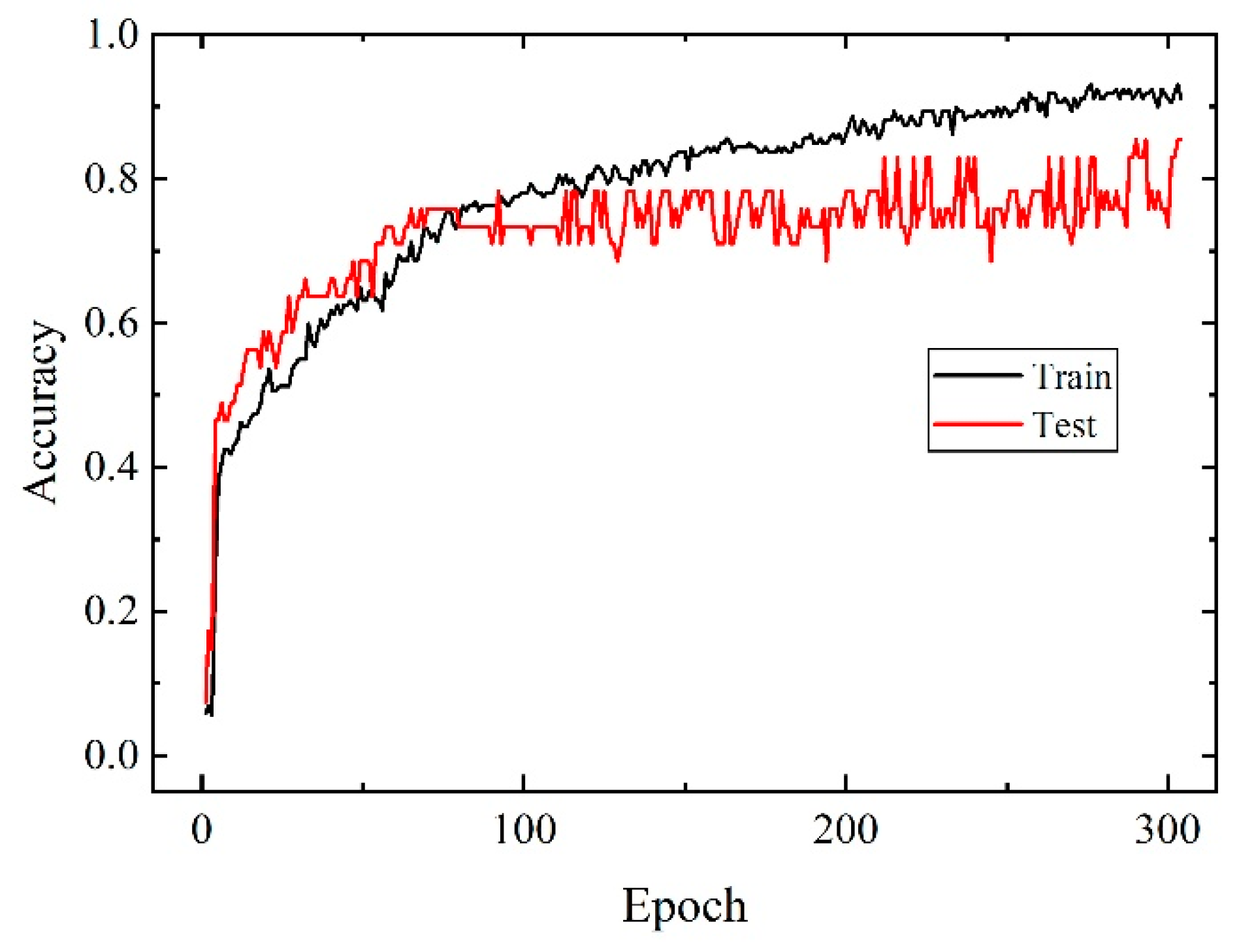
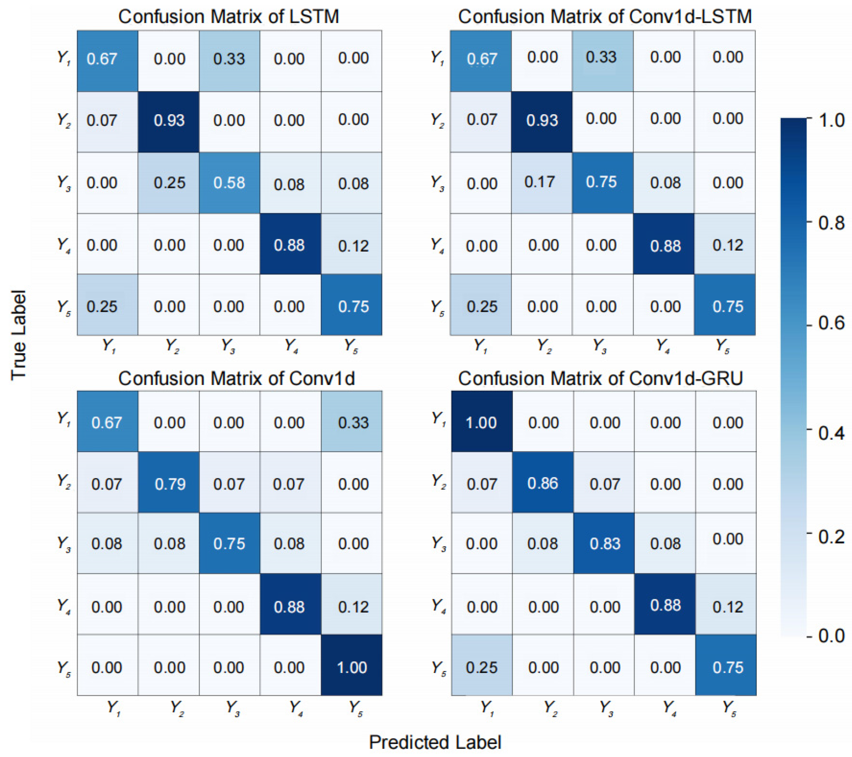
4.2. Comparative Analysis of Conv1d-GRU, GRU, LSTM, Conv1d, and Conv1d-LSTM Models

In this paper, the widely used GRU, LSTM, and Conv1d models and their combinations were selected and the performance of each model in this task was compared through experiments.

Table 5. Classification performance of the five models.

Models	Accuracy (%)	Weighted Precision (%)	Weighted Recall (%)
GRU	78.05%	79.94%	78.05%
LSTM	78.05%	82.74%	78.05%
Conv1d	80.49%	82.98%	80.49%
Conv1d-LSTM	82.93%	83.98%	82.93%
Conv1d-GRU	85.37%	86.91%	85.37%

lists the main evaluation metrics of the five models in the classification task, including accuracy, weighted precision, and weighted recall. The experimental results show that there are significant differences in classification performance between different models. Among them, the combined Conv1d + GRU model performs best in all indicators, with an accuracy of 85.37%, a weighted precision of 86.91%, and a weighted recall of 85.37%. In contrast, the accuracy of GRU and LSTM is 78.05%, and the overall performance is relatively low. Conv1d and Conv1d + LSTM perform in the middle, with an accuracy of 80.49% and 82.93%. The comprehensive analysis shows that the fusion of CNN, GRU, and LSTM can effectively improve the model’s ability to extract complex features so as to achieve better performance in the classification task of inrush water source discrimination.

To further evaluate the classification ability of each model on specific categories, Figure 5 shows the F1 scores of the five models in the five categories. Applying only 20% of the original data, the number of samples of each category in each test set is 3, 14, 12, 8, and 4. Thus, the 3 in Y₁ (3) represents the number of test sets for Y₁ categories. The results show that Conv1d-GRU performs well in all categories; the F1 score is between 0.75 and 0.89, especially in the Y₂, Y₃, and Y₄ categories, and it is concentrated from 0.87 to 0.89, showing good stability and generalization ability. In contrast, due to the small number of samples, the classification performance of the model on Y₁ and Y₅ categories is generally low, especially for Y₁.

Conv1d-LSTM also shows good performance in most categories, especially in the Y₂ and Y₄ categories, and its F1 score is close to that of Conv1d-GRU. In contrast, GRU and LSTM perform relatively poorly in the Y₁ and Y₃ categories, reflecting their limitations when dealing with partial category data.

From the category distribution, the number of samples in the Y₂, Y₃, and Y₄ categories is relatively large, the F1 scores of each model in these categories are generally high, and the performance is relatively stable. Among them, although the performance of multiple models on Y₂ and Y₄ is close, Conv1d-GRU still maintains a clear advantage in the Y₃ category with a large sample size, which has become a key factor for its overall performance lead.

This paper further presents a visualization of the classification results of the four models in Figure 6. According to the confusion matrix in Figure 6, both LSTM and Conv1d-LSTM models perform well on the Y₂ and Y₄ categories, and for the classification of Y₃, the LSTM model has a weak performance with an accuracy of 0.58. The performance of the Conv1d-LSTM model is improved, and the accuracy is improved to 0.75, showing better recognition ability for this category. Both Conv1d and Conv1D-GRU models have an accuracy of 1.00 on the Y₅ and Y₁ categories, but the results may be overfitting and the accuracy is not representative due to the small number of samples in these two categories. In addition, the Conv1d-GRU model shows a strong overall performance with high accuracy for categories Y₂, Y₃, and Y₄ with a large sample size.

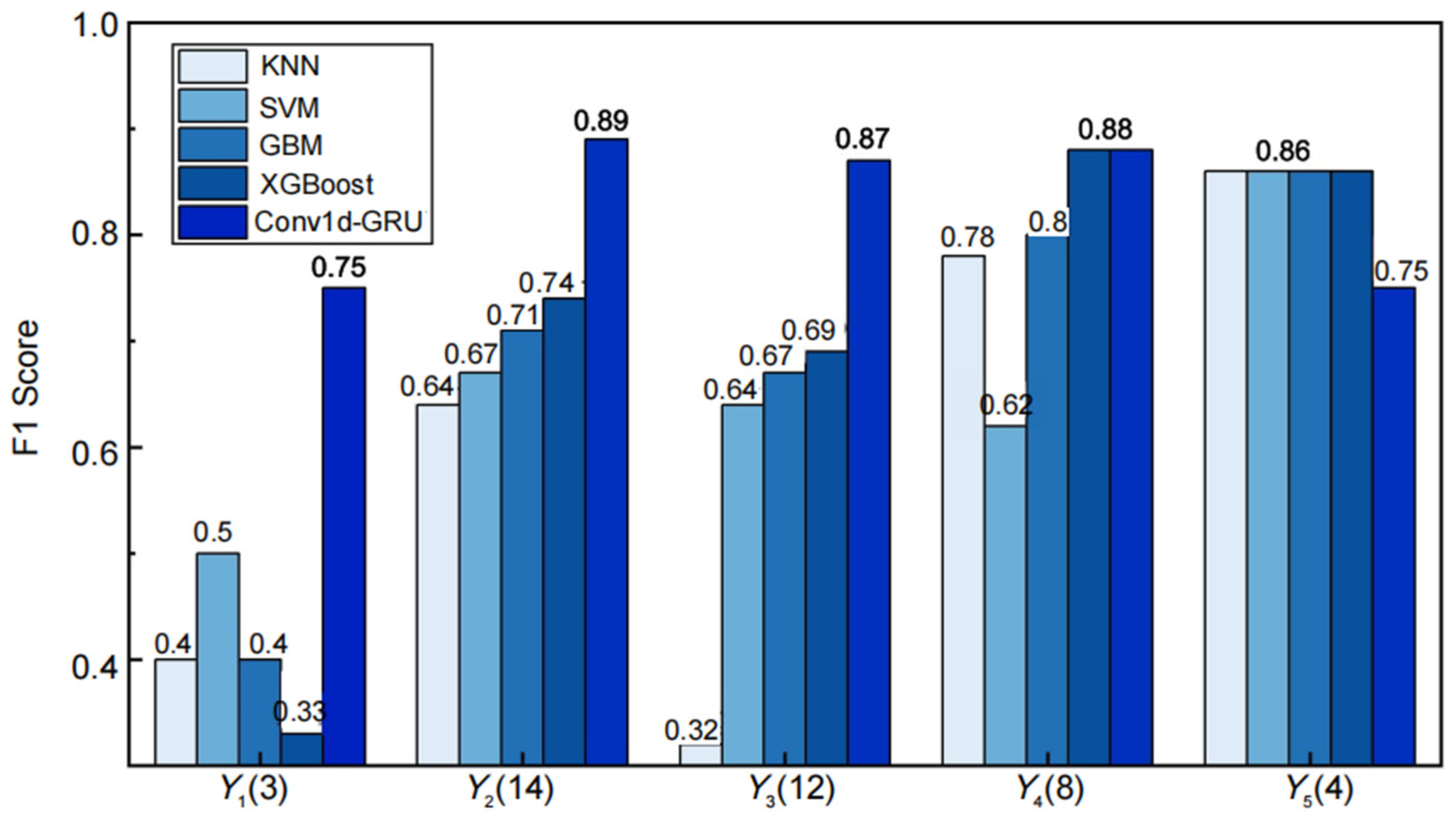
4.3. Comparative Analysis of Conv1d-GRU and Traditional Machine Learning Models

Using a comparison experiment, we further verified the performance of the Conv1d-GRU model compared with several traditional machine learning models. The relevant experimental results are listed in

Table 6. Classification performance of the eight models.

Models	Accuracy (%)	Weighted Precision (%)	Weighted Recall (%)
KNN	58.54%	60.00%	58.54%
SVM	65.85%	68.62%	65.85%
LightGBM	65.85%	69.91%	65.85%
RF	70.73%	75.85%	70.73%
ANN	70.73%	71.40%	70.73%
GBM	70.73%	71.75%	70.73%
XGBoost	73.17%	74.35%	73.17%
Conv1d-GRU	85.37%	86.91%	85.37%

. It can be seen that the proposed Conv1d-GRU model achieves significantly better results than the traditional model in all performance metrics. In the classification task of inrush water sources, the Conv1d-GRU model achieves the highest classification accuracy of 85.37%, which is far higher than other comparison models. Among them, the KNN model has the lowest accuracy of 58.54%. The accuracy of the SVM and LightGBM models was 65.85%, which was at a medium level. RF, ANN, and GBM had a relatively high accuracy of 70.73%. Among the traditional machine learning models, XGBoost performs the best, with an accuracy of 73.17%.

In terms of weighted accuracy, Conv1d-GRU reaches 86.91%, which is significantly better than other models. In the traditional model, RF has the highest accuracy of 75.85%. This result shows that Conv1d-GRU has a stronger ability to reduce misclassification, especially false positives. In terms of weighted recall rate, Conv1d-GRU also maintains a leading level of 85.37%, which is significantly higher than XGBoost (73.17%), further verifying its sensitivity and comprehensiveness in positive example identification.

In conclusion, the Conv1d-GRU model is superior to the traditional machine learning model in terms of accuracy, weighted precision, and weighted recall, showing higher stability and adaptability.

Considering that SVM and LightGBM have no significant difference in accuracy, and that RF, ANN, and GBM exhibit similar performance, this study selects KNN, SVM, GBM, and XGBoost as representatives to compare and analyze the F1 scores of the proposed Conv1d-GRU model across each category. It can be seen in Figure 7 that Conv1d-GRU leads in all categories, especially in the Y₂ category, with an F1 score of 0.89, which reflects its ability to model complex data structures.

The differences in F1 scores among the categories are evident. Notably, the F1 score of KNN in the Y₃ category is merely 0.32, significantly lower than that of other models, indicating its deficiency in capturing the features of this category. Conv1d-GRU, however, continues to exhibit strong performance in this category, with an F1 score of 0.87, demonstrating its robustness. While traditional models like XGBoost perform well in certain categories (such as Y₄), achieving an F1 score of 0.78, they still fall short of Conv1d-GRU’s score of 0.88, highlighting the constraints of traditional methods when handling high-dimensional and nonlinear features.

It is worth noting that Conv1d-GRU shows strong stability and consistency with small F1 score fluctuation among various classes, which is crucial for reliability in practical applications. However, the performance of traditional models fluctuates greatly on different categories, revealing their sensitivity to changes in data distribution.

Figure 8 illustrates the confusion matrices of the four traditional models, KNN, SVM, XGBoost, and Conv1d-GRU, to visually compare their classification performance in the multi-class task. The Conv1d-GRU model performs the best in terms of classification accuracy. In contrast, the accuracy of KNN on class Y₃ is only 0.25, reflecting the obvious shortcomings of the model when dealing with samples from this category.

The misclassification rates of Conv1d-GRU in all categories are low, especially in the Y₃ and Y₂ categories, where the misclassification rates of Conv1D-GRU are only 0.08 and 0.07, which are significantly better than the misclassification rates of 0.25 and 0.14 in the SVM Y₃ and Y₂ categories. In addition, Conv1d-GRU performs more evenly across all categories, and the classification accuracy fluctuates less. However, the accuracy of XGBoost on categories Y₂ and Y₃ is 0.71 and 0.75, and there is a certain degree of performance fluctuation, indicating that the classification ability of the model is slightly unstable between different categories.

In summary, the Conv1d-GRU model is superior to the other three comparison models in terms of classification accuracy, misclassification control ability, and overall stability, showing its significant advantages in multi-class classification tasks.

5. Explainable Machine Learning Model for Source Type Identification of Mine Inrush Water

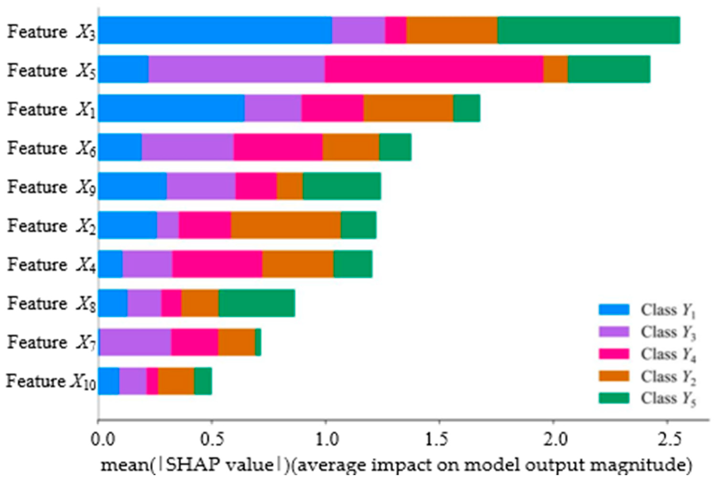
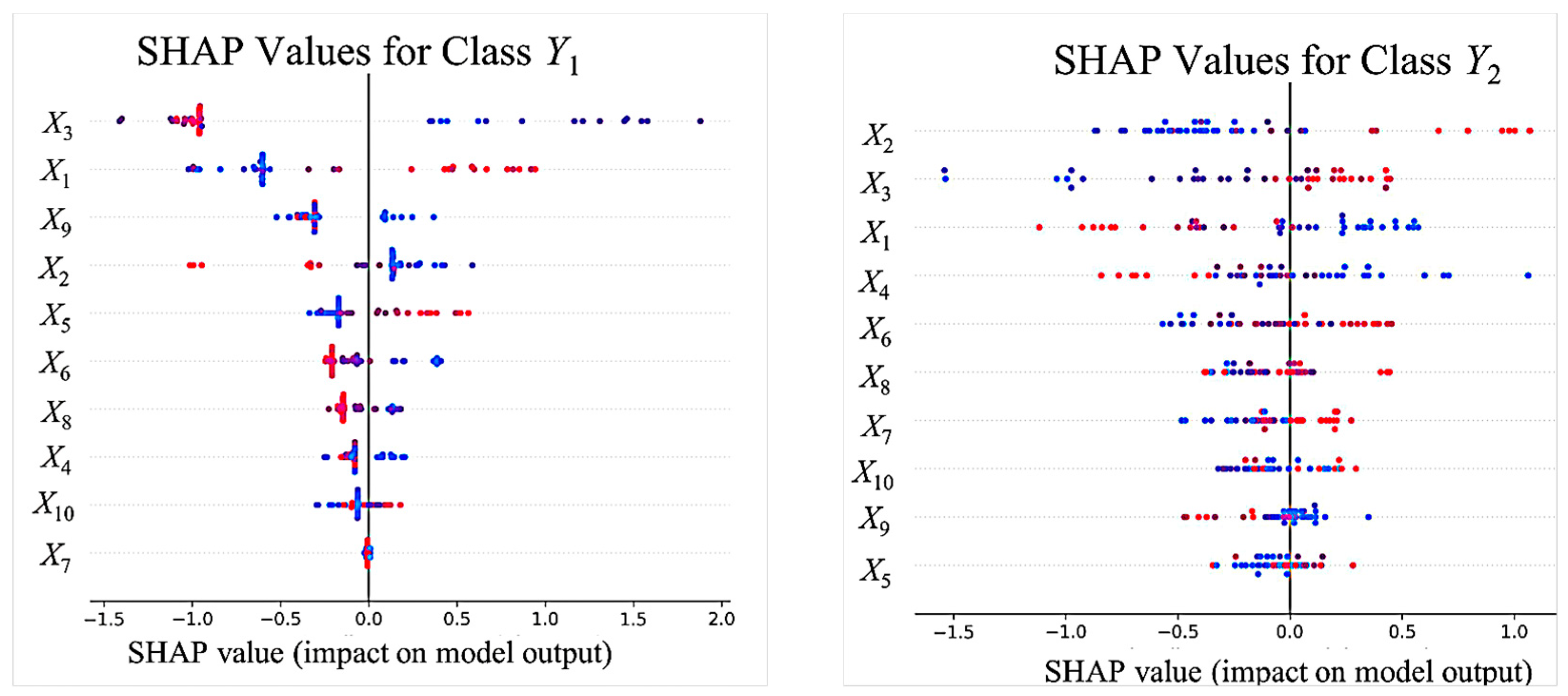
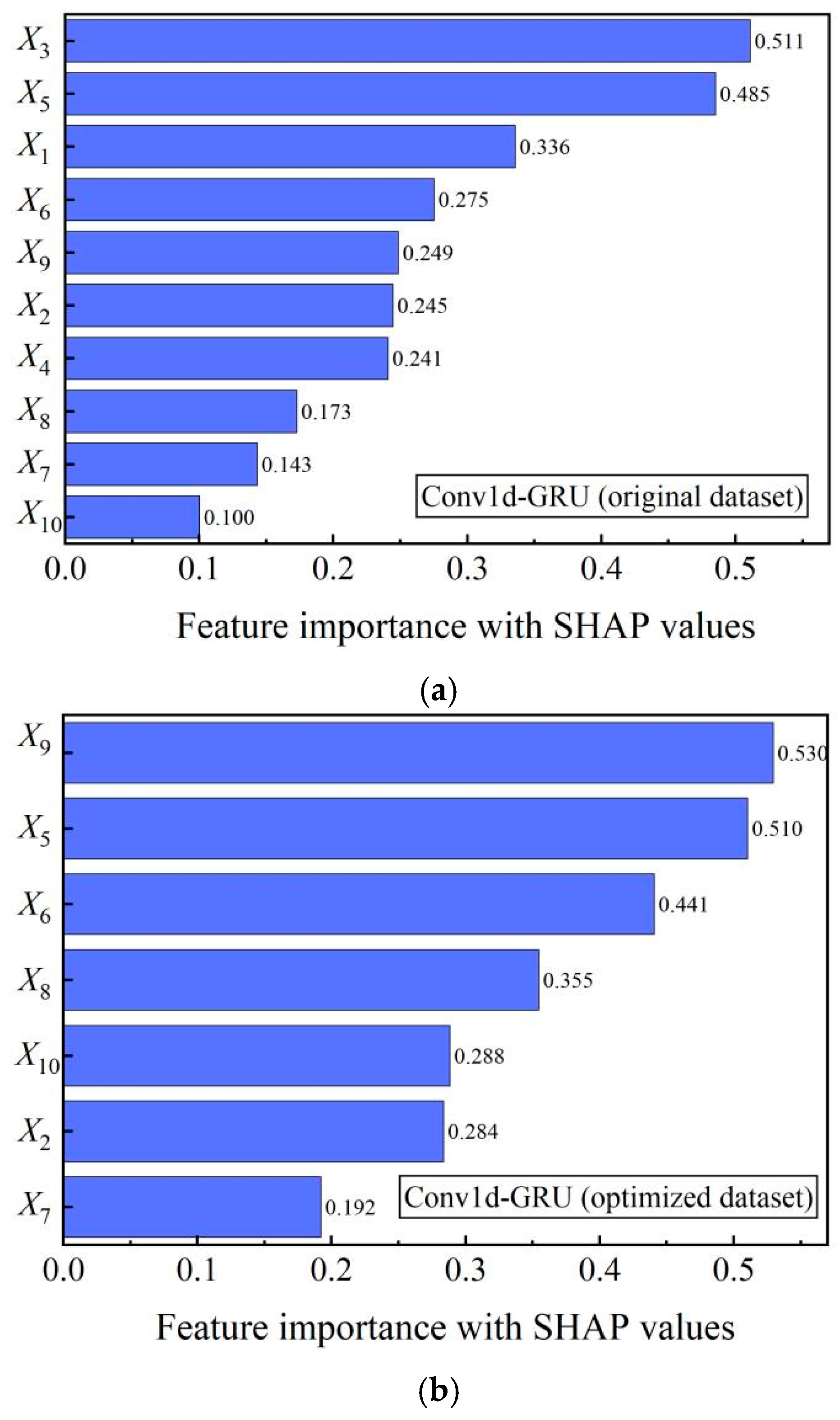
5.1. Interpretability Analysis Using SHAP Values

To enhance the transparency and credibility of the model, this paper conducts a detailed interpretability analysis of the Conv1d-GRU multi-classification model using SHAP (SHapley Additive exPlanations) values. SHAP values, as an effective tool for assessing feature importance, can quantify the contribution of each feature in the model output and take into account the interactions between features. By understanding the decision-making mechanism of the model in each category through the SHAP method, the experimental results are shown in Figure 9 and Figure 10.

Figure 9 presents the average SHAP values for all features, as well as the overall impact of the features on the model output. The x-axis represents the average absolute SHAP value, and the y-axis displays the features sorted in descending order of importance. The colors indicate the water quality categories (Y₁–Y₅). It can be seen that all features work together to realize the identification of water sources. The ranking of feature importance for the model is as follows: $\mathrm{N}{\mathrm{a}}^{+}/{\mathrm{K}}^{+}$ (X₃), $\mathrm{S}{\mathrm{O}}_4^{2-}$ (X₅), $\mathrm{C}{\mathrm{a}}^{2+}$ (X₁), $\mathrm{C}{\mathrm{l}}^{-}$ (X₆), alkalinity (X₉), $\mathrm{M}{\mathrm{g}}^{2+}$ (X₂), ${\mathrm{HCO}}_3^{-}$ (X₄), TDS (X₈), pH (X₇), and hardness (X₁₀). Experimental results show that features X₃, X₅, and X₁ all exhibit relatively high average SHAP values across all categories, indicating that these features have a significant influence on the model’s prediction results.

The average absolute SHAP values of $\mathrm{N}{\mathrm{a}}^{+}/{\mathrm{K}}^{+}$ (X₃) were the highest (approximately 2.5), exerting the strongest influence on the model output. In the Aohui Water (Y₁, blue) and the Cenozoic Aquifer Water (Y₅, green), the concentrations of $\mathrm{N}{\mathrm{a}}^{+}/{\mathrm{K}}^{+}$ were positively correlated with the weathering degree of the strata minerals. Due to the presence of Ordovician limestone (such as sodium feldspar, potassium feldspar, etc.), the fourth-order loose sediments of the Neogene (such as clay minerals like montmorillonite, illite, etc.) are rich in $\mathrm{N}{\mathrm{a}}^{+}/{\mathrm{K}}^{+}$ minerals. During the long-term interaction between water and rock, the minerals gradually dissolve and release a large amount of $\mathrm{N}{\mathrm{a}}^{+}/{\mathrm{K}}^{+}$.

$\mathrm{S}{\mathrm{O}}_4^{2-}$ (X₅) ranks second in importance for influencing the model output, with an approximate value of 2.2, and it demonstrates a significant positive contribution in the Goaf Water (Y₃, purple) and the Taihui Water (Y₄, pink). This is primarily due to the exposure of sulfur-containing substances in the coal layer to air or contact with water during coal mining. The sulfur elements in the coal undergo processes such as oxidation, which produce sulfate ions. These ions then enter the dark gray water system via mine drainage.

The average absolute SHAP value of $\mathrm{C}{\mathrm{a}}^{2+}$ (X₁) is approximately 1.8, indicating a moderate impact on the model output. It plays a significant role in the Aohui Water (Y₁, blue) and Sandstone Water (Y₂, brown). The higher $\mathrm{C}{\mathrm{a}}^{2+}$ concentration in water is often closely related to karst development, reflecting the strength of rock dissolution. The Ordovician Limestone is mainly composed of carbonate minerals such as calcium carbonate. Sandstone Water is mostly found in carbonate-cemented sandstone.

The SHAP values of ${\mathrm{HCO}}_3^{-}$ (X₄) and alkalinity (X₉) are close to each other in the order of feature importance, and their influence direction on model output is completely consistent.

Figure 10 shows the distribution of SHAP values for the features in different categories. In the SHAP distribution plot, the horizontal axis represents the influence of the feature on the category prediction (SHAP value), with positive values indicating promotion and negative values indicating inhibition of the category prediction; the vertical axis represents the feature names, and the color gradient reflects the feature values (red indicating high and blue indicating low). By analyzing the SHAP distribution patterns of the features, the association mechanism between different water quality categories and water chemical characteristics can be revealed.

The model not only relies on high-impact features, but also needs to independently model the responses of features in different categories. From the results of the category contribution, it can be seen that the Aohui Water (Y₁, blue) is associated with $\mathrm{N}{\mathrm{a}}^{+}/{\mathrm{K}}^{+}$ (X₃), $\mathrm{C}{\mathrm{a}}^{2+}$ (X₁), and alkalinity (X₉). The positive SHAP values of $\mathrm{N}{\mathrm{a}}^{+}/{\mathrm{K}}^{+}$ are mainly concentrated in the range of 0–2.0 and contribute significantly. The positive SHAP values of $\mathrm{C}{\mathrm{a}}^{2+}$ are concentrated in the range of 0–1.5, and they work in synergy with X₃. The positive SHAP values of alkalinity are mostly within the range of 0–1.0. A small number of positive SHAP values of $\mathrm{S}{\mathrm{O}}_4^{2-}$ fall within the range of 0–0.5, while the negative SHAP values are very weak. Thus, the positive contributions of $\mathrm{N}{\mathrm{a}}^{+}/{\mathrm{K}}^{+}$ validate the core role of carbonate rock dissolution; the positive contribution of Alkalinity validates the dominant source of alkalinity being bicarbonate; and the weak contribution of $\mathrm{S}{\mathrm{O}}_4^{2-}$ validates the restricted oxidation of pyrite in the Aohui Water environment.

The Sandstone Water (Y₂, brown) is associated with $\mathrm{M}{\mathrm{g}}^{2+}$(X₂), $\mathrm{C}{\mathrm{a}}^{2+}$(X₁), and $\mathrm{N}{\mathrm{a}}^{+}/{\mathrm{K}}^{+}$(X₃). The positive SHAP values of $\mathrm{M}{\mathrm{g}}^{2+}$ are mainly concentrated in the range of 0–1.0 and the high feature values contribute significantly. The weak negative/positive SHAP values of $\mathrm{C}{\mathrm{a}}^{2+}$ and $\mathrm{N}{\mathrm{a}}^{+}/{\mathrm{K}}^{+}$ are concentrated in the −1.5 to 0.5 range, indicating a weak contribution. The positive contribution of $\mathrm{M}{\mathrm{g}}^{2+}$ verifies the dominant role of magnesium clay in the cementation of sandstone. The weak contribution of $\mathrm{C}{\mathrm{a}}^{2+}$ and $\mathrm{N}{\mathrm{a}}^{+}/{\mathrm{K}}^{+}$ confirms the lithological background of low carbonate mineral content in sandstone.

The Goaf Water (Y₃, purple) is associated with $\mathrm{S}{\mathrm{O}}_4^{2-}$ (X₅), ${\mathrm{Cl}}^{-}$ (X₆), and pH (X₇). The SHAP values of $\mathrm{S}{\mathrm{O}}_4^{2-}$ are distributed in both the positive contribution range (0–0.5) and the negative contribution range (−1.5–0). There are many high-eigenvalue points, and the core contribution is significant. The positive and negative values of the SHAP values of $\mathrm{C}{\mathrm{l}}^{-}$ are scattered and concentrated within the range of −1.0 to 0.5, and the contribution is scattered. Both positive and negative values of pH exist. The negative contribution (−1.5–0) is concentrated at a point, and there are many high eigenvalues. These are the key chemical boundaries for identifying this category. Thus, the strong contributions of $\mathrm{S}{\mathrm{O}}_4^{2-}$ and pH in verifying the oxidation mechanism of pyrite are quantitative manifestations of the oxidation of pyrite caused by coal mining. The abandoned areas may be affected by the dissolution of a small amount of rock salt (NaCl) in the coal-bearing strata, or by the mixing of mine water with domestic/industrial chlorinated wastewater. $\mathrm{C}{\mathrm{l}}^{-}$ ions have certain sources.

The Taihui Water (Y₄, pink) is associated with $\mathrm{S}{\mathrm{O}}_4^{2-}$ (X₅), ${\mathrm{HCO}}_3^{-}$ (X₄), and $\mathrm{C}{\mathrm{l}}^{-}$ (X₆). Positive and negative SHAP values of $\mathrm{S}{\mathrm{O}}_4^{2-}$ are both present. The negative contribution range (−2.0–0) is densely concentrated, while the positive contribution (0–1.0) is only slightly present. The positive SHAP value of ${\mathrm{HCO}}_3^{-}$ dominates (in the 0–1.0 range), with a large number of high feature values, and it is the core indicator of chemical characteristics. The $\mathrm{C}{\mathrm{l}}^{-}$ values are dispersed with a concentration in the range of −0.5 to 1.0, and their auxiliary role in identifying turbid water is weak, with a scattered contribution. The conclusion is that the Taihui Water has a negative SHAP value of $\mathrm{S}{\mathrm{O}}_4^{2-}$, indicating low sulfate inhibition and that is a “calcium bicarbonate-type” sludge water.

The Cenozoic Aquifer Water (Y₅, green) is associated with $\mathrm{N}{\mathrm{a}}^{+}/{\mathrm{K}}^{+}$ (X₃), $\mathrm{S}{\mathrm{O}}_4^{2-}$ (X₅), and alkalinity (X₉). The positive and negative SHAP values of $\mathrm{N}{\mathrm{a}}^{+}/{\mathrm{K}}^{+}$ are distributed in the range of −1.0 to 1.5, and the high feature values contribute significantly. The positive and negative SHAP values of $\mathrm{S}{\mathrm{O}}_4^{2-}$ and alkalinity are distributed in the range of −0.5 to 0.5, with a moderate contribution. From this, it can be concluded that the distribution of SHAP values for the Cenozoic aquifer water and the high variability of $\mathrm{N}{\mathrm{a}}^{+}/{\mathrm{K}}^{+}$, $\mathrm{S}{\mathrm{O}}_4^{2-}$, and alkalinity reflect the “quaternary loose layer + human activities superimposition” process, driving the model to predict Y₅.

5.2. Comparative Analysis of the Interpretability of Feature Importance When Selecting Features

Based on hydrogeological research, TDS (X₈) represents the total amount of all inorganic ions dissolved in water. In natural water bodies, $\mathrm{N}{\mathrm{a}}^{+}/{\mathrm{K}}^{+}$ (X₃) is usually one of the main contributors to TDS, showing a high correlation with TDS. ${\mathrm{HCO}}_3^{-}$ (X₄) is the dominant element in the formation of alkalinity (X₉) and statistically shows a significant positive correlation. This reflects the intrinsic connection between “water–rock interactions” and the “carbon cycle” in hydrogeological processes. In natural water bodies, $\mathrm{C}{\mathrm{a}}^{2+}$ (X₁) and $\mathrm{M}{\mathrm{g}}^{2+}$ (X₂) show an extremely strong positive correlation with hardness (X₁₀).

Through feature correlation analysis, this paper eliminated features X₁, X₃, and X₄ and constructed an optimized feature database. As expected, the experimental results showed that the classification accuracy of the proposed model remained unchanged when using the optimized database. To further explore the impact of the eliminated features on the model, this paper used the SHAP method to conduct interpretive analysis and ranking of the importance of each feature.

Figure 11 shows the distribution of feature importance calculated based on SHAP values in both the original dataset and the optimized dataset. Compared with the original dataset, the importance values of all features in the optimized dataset have increased. This indicates that after reducing feature redundancy, each remaining feature plays a more prominent role in the model’s decision-making. Specifically, the SHAP values of feature X₉, X₅, and X₆ are 0.530, 0.510, and 0.441, respectively, indicating that they dominate in the optimized dataset.

It is worth noting that although the classification accuracy remained unchanged, the importance of feature X₉ significantly increased. This result indicates that feature X₉ has enhanced its contribution to the classification in the optimized database, effectively compensating for the roles of the removed features (X₁, X₃, and X₄) in the original dataset, thereby improving the efficiency of feature utilization while maintaining the stability of the model performance.

6. Conclusions

The rapid and accurate identification of the source type of mine inrush water is a crucial aspect of mine water prevention and control. To address the current problem of insufficient information acquisition and identification methods for inrush water precursors, this paper proposes an explainable machine learning model for source type identification of mine inrush water. The research is conducted considering three aspects: the water chemical characteristics of different aquifers, the discriminant factors of the water source, and explainable source identification models. It achieves better performance in the task of inrush water source classification. However, the geological conditions in China are much more complex than those modeled, and regional aquifers have obvious differences. This study only expands the original monitoring scope to Xinxijiu Mine as the research sample and has achieved certain results. In later research, it is hoped that data samples from different terrain areas can be used as research objects to verify and optimize the inrush water discrimination model.

References

1. Jiang, Q.; Liu, Q.; Liu, Y.; Chai, H.; Zhu, J. Groundwater chemical characteristic analysis and water source identification model study in Gubei coal mine, Northern Anhui Province, China. Heliyon 2024, 10, 26925. [Google Scholar] [CrossRef] [PubMed]
2. Chitsazan, M.; Heidari, M.; Ghobadi, M. The Study of the Hydrogeological Setting of the Chamshir Dam Site with Special Emphasis on the Cause of Water Salinity in the Zohreh River Downstream from the Chamshir Dam (Southwest of Iran). Environ. Earth Sci. 2012, 67, 1605–1617. [Google Scholar] [CrossRef]
3. Zhang, J. Investigations of water inrushes from aquifers under coal seams. Int. J. Rock Mech. Min. Sci. 2005, 42, 350–360. [Google Scholar] [CrossRef]
4. Tijani, M.N. Contamination of shallow groundwater system and soil–plant transfer of trace metals under amended irrigated fields. Agric. Water Manag. 2009, 96, 437–444. [Google Scholar] [CrossRef]
5. Shi, L.Q. Summary of research on mechanism of water inrush from seam floor. J. Shandong Univ. Sci. Technol. 2009, 28, 17–23. [Google Scholar]
6. Fazzino, F.; Roccaro, P.; Di Bella, A. Use of fluorescence for real-time monitoring of contaminants of emerging concern in (waste) water: Perspectives for sensors implementation and process control. J. Environ. Chem. Eng. 2025, 13, 115916. [Google Scholar] [CrossRef]
7. Milinovic, J.; Santos, P.; Marques, J.E. Spectroscopic signatures for expeditious monitoring of contamination risks at abandoned coal mine sites. Geochemistry 2025, 85, 126292. [Google Scholar] [CrossRef]
8. Dong, F.; Yin, H.; Cheng, W.; Zhang, C.; Zhang, D.; Ding, H.; Lu, C.; Wang, Y. Quantitative prediction model and prewarning system of water yield capacity (WYC) from coal seam roof based on deep learning and joint advanced detection. Energy 2024, 290, 130200. [Google Scholar] [CrossRef]
9. He, C.Y.; Zhou, M.R.; Yan, P.C. Application of the Identification of Mine Water Inrush with LIF Spectrometry and KNN Algorithm Combined with PCA. Spectrosc. Spectr. Anal. 2016, 36, 2234–2237. [Google Scholar]
10. Yao, D.; Chen, S.; Qin, D.J. Modeling abrupt changes in mine water inflow trends: A CEEMDAN-based multi-model prediction approach. J. Clean. Prod. 2024, 439, 140809. [Google Scholar] [CrossRef]
11. Yin, H.; Wu, Q.; Yin, S.; Dong, S.; Dai, Z.; Soltanian, M.R. Predicting mineinrush water accidents based on water level anomalies of borehole groups using long short-term memory and isolation forest. J. Hydrol. 2023, 616, 128813. [Google Scholar] [CrossRef]
12. Shi, L.; Qu, X.; Han, J.; Qiu, M.; Gao, W.; Qin, D.; Liu, H. Multi-model fusion for assessing risk of inrush of limestone karst water through the mine floor. Energy Rep. 2021, 7, 1473–1487. [Google Scholar] [CrossRef]
13. Ma, J.; Zhang, Y. A New Dynamic Assessment for Multi-parameters Information ofinrush water in Coal Mine*. Energy Procedia 2012, 16, 1586–1592. [Google Scholar]
14. Li, D.; Peng, S.; Guo, Y.; Lin, P. Development status and prospect of geological guarantee technology for intelligent coal mining in China. Green Smart Min. Eng. 2024, 1, 433–446. [Google Scholar] [CrossRef]
15. Zhao, Y.; Zhang, L.; Chen, Y. Water environment risk prediction method based on convolutional neural network-random forest. Mar. Pollut. Bull. 2024, 209, 117228. [Google Scholar] [CrossRef] [PubMed]
16. Zhao, W.; Wan, Y.; Wang, K.; Zhao, Z.; Song, Y.; Guo, X.; Xiang, G. Methods for constructing scenarios of coal and gas outburst accidents: Implications for the intelligent emergency response of secondary mine accidents. Process Saf. Environ. Prot. 2025, 199, 107236. [Google Scholar] [CrossRef]
17. Tong, X.; Zheng, X.; Jin, Y.; Dong, B.; Liu, Q.; Li, Y. Prevention and control strategy of coal mine water inrush accident based on case-driven and Bow-tie-Bayesian model. Energy 2025, 320, 135312. [Google Scholar] [CrossRef]
18. Ouifak, H.; Idri, A. A comprehensive review of fuzzy logic based interpretability and explainability of machine learning techniques across domains. Neurocomputing 2025, 647, 130602. [Google Scholar] [CrossRef]
19. Moghaddas, S.A.; Bao, Y. Explainable machine learning framework for predicting concrete abrasion depth. Case Stud. Constr. Mater. 2025, 22, e04686. [Google Scholar] [CrossRef]
Figure 1. Ion concentration contrast diagram of each aquifer.
Information 16 00648 g001
Figure 2. Correlation coefficient of characteristics.
Information 16 00648 g002
Figure 3. Model construction.
Information 16 00648 g003
Figure 4. Comparison curve of training and validation accuracy rates.
Information 16 00648 g004
Figure 5. F1 score of the GRU, LSTM, Conv1d, Conv1d + LSTM, and Conv1d + GRU models.
Information 16 00648 g005
Figure 6. Confusion matrices for LSTM, Conv1d-LSTM, Conv1d, and Conv1d-GRU models.
Information 16 00648 g006
Figure 7. F1 score of KNN, SVM, GBM, XGBoost, and the proposed model.
Information 16 00648 g007
Figure 8. Confusion matrices for the KNN, SVM, XGBoost, and Conv1d-GRU models.
Information 16 00648 g008
Figure 9. An interpretability analysis diagram of feature importance.
Information 16 00648 g009
Figure 10. Distribution chart of SHAP values for features of different categories in the multi-classification model.
Information 16 00648 g010aInformation 16 00648 g010b
Figure 11. Global feature importance (a) based on the original data (b) based on the database after eliminating the features.
Information 16 00648 g011