Adaptive Multi-Gradient Guidance with Conflict Resolution for Limited-Sample Regression

Abstract

Recent studies report that gradient guidance extracted from a single-reference model can improve Limited-Sample regression. However, one reference model may not capture all relevant characteristics of the target function, which can restrict the capacity of the learner. To address this issue, we introduce the Multi-Gradient Guided Network (MGGN), an extension of single-gradient guidance that combines gradients from several reference models. The gradients are merged through an adaptive weighting scheme, and an orthogonal-projection step is applied to reduce potential conflicts between them. Experiments on sine regression are used to evaluate the method. The results indicate that MGGN achieves higher predictive accuracy and improved stability than existing single-gradient guidance and meta-learning baselines, benefiting from the complementary information provided by multiple reference models.

1. Introduction

Rapid developments in artificial intelligence have brought Limited-Sample learning into a number of application areas, including industrial manufacturing, medical diagnosis, and hydrological forecasting [1,2,3]. Limited-Sample methods exploit prior knowledge so that new tasks can be handled with only a small amount of labeled data [4,5,6]. These approaches leverage prior knowledge through various mechanisms: learning transferable representations across tasks, constructing prototype-based metric spaces for rapid classification, and employing attention-driven matching between support sets and query samples. Such strategies enable effective generalization from minimal supervised examples by incorporating structural knowledge from related domains or pre-trained models.Within this domain, Limited-Sample regression focuses on obtaining accurate numerical predictions under data scarcity.

Current solutions can be grouped into model fine-tuning [7,8], meta-learning [9,10,11,12], and data augmentation [13]. Fine-tuning may overfit when data are limited, meta-learning generally requires many related tasks, and augmentation may introduce additional noise. Consequently, combining learning algorithms with mechanistic or domain models has become an active research direction for Limited-Sample regression.

If a differentiable theoretical model is available, its gradient can be added as a training constraint [14], thereby reducing the effect of data scarcity. A single-reference model, however, may not capture all aspects of a complex target function. While multiple reference models provide diverse gradient information, they also introduce the challenge of merging potentially conflicting directions while resolving possible inconsistencies.

The present work studies this multi-gradient setting and makes three observations:

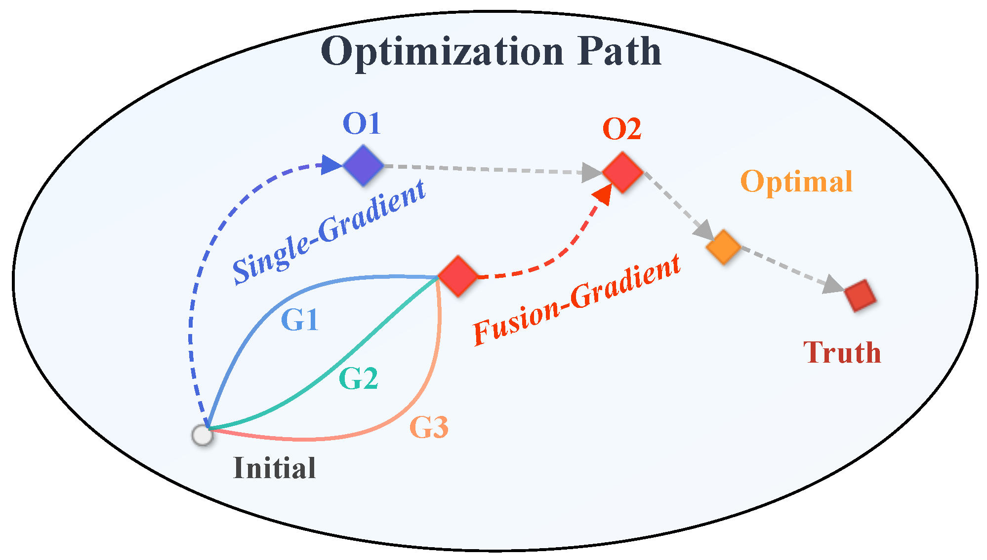
• Different reference models contribute gradients that emphasize distinct characteristics of the objective.
• Combining these gradients can retain useful directions from each model and offset individual biases.
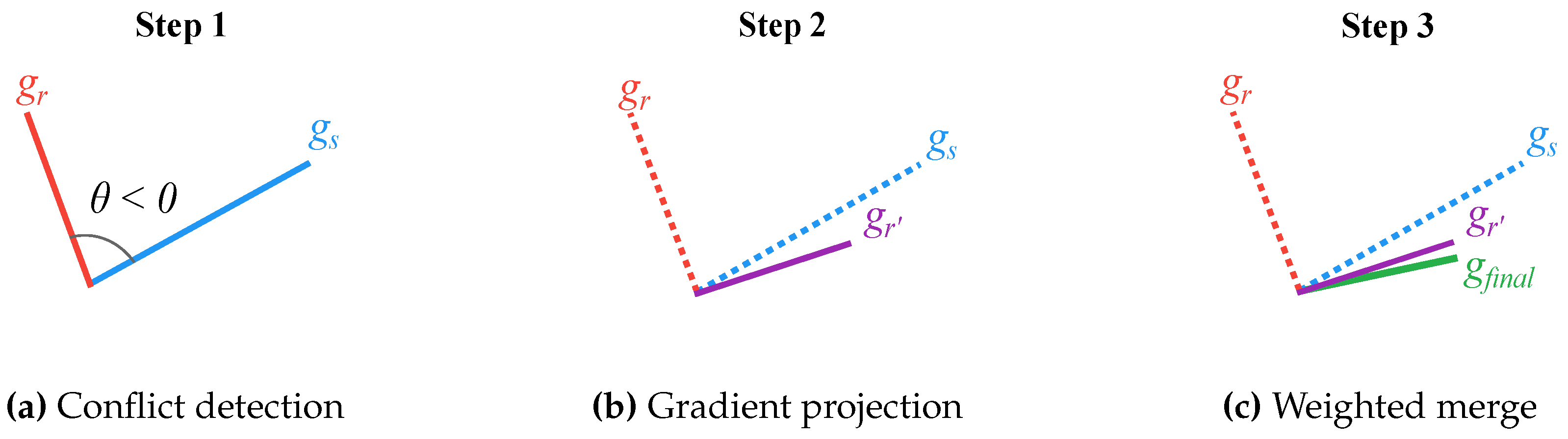
• An effective fusion rule should consider both directional agreement and the relative importance of each source.

To realize these ideas, we start from the Gradient Guided Network (GGN) and extend it to a Multi-Gradient Guided Network (MGGN). MGGN assigns adaptive weights to the gradients of several reference models and applies an orthogonal-projection step to limit conflicts [14,15,16,17]. This gradient surgery approach treats multi-model learning as a multi-objective optimization problem, where conflicting gradients are resolved through projection operations that preserve beneficial update directions while mitigating interference. Figure 1 contrasts the optimization paths of single- and multi-gradient training.

The approach is evaluated on one-dimensional sine regression and is compared with representative baselines: GGN, DKT, MAML, Loo2019, and DNNFineTuning [14,18,19,20,21]. Experiments show consistent improvements in prediction accuracy and variance reduction.

The remainder of the paper is organized as follows. Section 2 reviews related work; Section 3 presents the method; Section 4 reports empirical results; Section 5 concludes.

2. Related Works

The field of Limited-Sample regression has experienced substantial growth in recent years, with research contributions spanning three primary categories: meta-learning methodologies, prior knowledge integration techniques, and domain-specific applications.

Meta-Learning Approaches in Limited-Sample Regression. Meta-learning frameworks leverage transferable knowledge across multiple tasks to facilitate rapid adaptation with minimal training data. Within Limited-Sample regression, numerous studies have adopted this approach. Baik et al. [22] developed the ALFA model, a meta-learning framework that generates task-adaptive hyperparameters through a lightweight meta-network responsive to current learning dynamics. This methodology demonstrated enhanced performance across diverse Limited-Sample regression benchmarks, highlighting the significance of adaptive optimization within meta-learning paradigms. Patacchiola et al. [18] introduced Deep Kernel Transfer (DKT), which combines Gaussian processes with deep neural networks through learned deep kernel functions for feature extraction. While achieving competitive results, DKT demonstrates considerable sensitivity to kernel selection. Addressing this limitation, Savaşlı et al. [23] systematically evaluated multiple kernel functions and optimizers, establishing that kernel choice significantly impacts model performance and providing optimization guidelines.

Prior Knowledge Integration in Limited-Sample Regression. The incorporation of domain-specific knowledge represents an effective strategy for enhancing performance and generalization in Limited-Sample regression. Various approaches have emerged to combine theoretical models with data-driven methodologies. Loo et al. [19] developed a method for learning function representations using basis functions derived from limited samples, demonstrating effectiveness in sine function prediction and validating the utility of basis function learning in data-constrained scenarios. The TADAM framework [24] extended this work by incorporating task-adaptive metrics to improve performance. Sui et al. [25] addressed lithium-ion battery lifespan prediction through early prediction schemes combining Limited-Sample learning with physical model knowledge, achieving accurate lifetime estimation using data from only six charging cycles. In multi-stage manufacturing quality prediction, Zhang et al. [1] proposed the Contrastive Decoder Generator (CDG), integrating contrastive learning with Limited-Sample approaches to leverage inter-stage correlations and substantially improve prediction accuracy under data limitations.

Domain Applications of Limited-Sample Regression. Limited-Sample regression methodologies have found successful implementation across multiple domains, including smart grid systems, hydrological modeling, and Internet of Things (IoT) environments. For smart grid applications, Xu et al. [26] introduced BiLO-Auto-TSF/ML, an automated meta-learning framework utilizing Bayesian bilevel optimization with upper-level hyperparameter optimization and lower-level meta-learning deployment. This approach significantly improved power load forecasting accuracy while addressing time-series prediction challenges in data-scarce environments. In hydrological applications, Yang et al. [3] developed a model combining metric learning with LSTM networks for runoff prediction in data-limited regions, demonstrating robust performance in Yellow River upstream area predictions and confirming the practical applicability of Limited-Sample regression methods. Within IoT contexts, studies by Hou et al. [27] and Chen et al. [28] proposed Limited-Sample learning solutions for WiFi-based indoor crowd counting and localization, achieving reliable performance despite environmental variability through effective utilization of minimal labeled data. Tian and Xie [29] contributed an adversarial meta-training framework for cross-domain Limited-Sample learning, incorporating adversarial training to enhance generalization capabilities across unseen domains and tasks.

3. Multi-Gradient Guided Network for Limited-Sample Regression

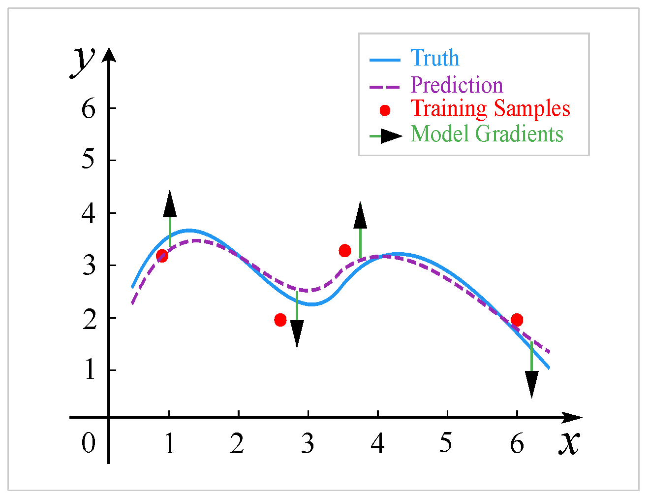
3.1. Gradient-Guided Limited-Sample Regression

Limited-Sample regression aims to learn an unknown function $F\left(x\right)$ from a limited labeled dataset $D_{\mathrm{train}}=\{(x_k,y_k)\mid k=1,\dots ,K\}$, where K is substantially smaller than conventional deep learning requirements. This task presents significant challenges due to high-dimensional function spaces and solution uncertainty [30]. The GGN [14] addresses this by incorporating gradient information from theoretical reference models as structured prior knowledge, formulating the optimization objective shown in Equation (1):

$$\underset{\theta }{min}L=L_p+\alpha L_g,$$

(1)

where

$$L_p=\sum _{k=1}^K{\left(M(x_k;\theta )-y_k\right)}^2,$$

(2)

$$L_g=\sum _{j=1}^N{∥{\nabla }_{x}M(x_j;\theta )-{\nabla }_{x}g\left(x_j\right)∥}^2.$$

(3)

Here, $M(x;\theta )$ represents the learned regression model, $g\left(x\right)$ denotes the scalar-valued reference model, N indicates the number of gradient sampling points, and $\alpha$ balances prediction loss and gradient constraints. Figure 2 demonstrates the gradient-guided network training process, where “Truth” indicates the target function $F\left(x\right)$ and “Prediction” represents the network output $M(x;\theta )$.

To exploit complementary information from multiple theoretical reference models, we introduce the MGGN framework. This approach aggregates gradient information from R reference models ${\left\{g_r\left(x\right)\right\}}_{r=1}^R$, with each model providing $N_r$ gradient sampling points. The loss function becomes as shown in Equation (4):

$$\underset{\theta }{min}L=L_p+\alpha L_{mg},$$

(4)

where

$$L_{mg}=\sum _{r=1}^R\sum _{j=1}^{N_r}{∥{\nabla }_{x}M(x_j;\theta )-{\nabla }_x{g}_r\left(x_j\right)∥}^2.$$

(5)

This multi-model integration strengthens prior constraints while introducing gradient conflict challenges addressed in the following section.

3.2. Multi-Gradient Fusion

To address gradient direction inconsistencies from multiple sources, we develop a multi-gradient fusion framework based on PCGrad [15].

For each sample $x_j$, the fused gradient is computed as shown in Equation (6):

$$g_{\mathrm{final}}\left(x_j\right)=\sum _{r=1}^R{w}_r{g}_r^{\prime }\left(x_j\right),$$

(6)

where $g_r^{\prime }\left(x_j\right)$ represents the gradient from the rth reference model after conflict resolution and orthogonal projection, with weights $w_r$ satisfying ${\sum }_{r=1}^R{w}_r=1$. For batch updates, the overall fused gradient is as shown in Equation (7):

$$g_{\mathrm{final}}={\displaystyle \frac{1}{{\sum }_{r=1}^R{N}_r}}\sum _{r=1}^R\sum _{j=1}^{N_r}{g}_{\mathrm{final}}\left(x_j\right).$$

(7)

Gradient conflicts are detected by computing inner products between gradients from different reference models, as shown in Equation (8):

$$c_{rs}=g_r·g_s<0.$$

(8)

When conflicts occur ($c_{rs}<0$), orthogonal projection is applied to $g_r$ as shown in Equation (9):

$$g_r^{\prime }=g_r-{\displaystyle \frac{g_r·g_s}{\parallel g_s{\parallel }^2}}{g}_s.$$

(9)

To account for varying sample coverage across reference models, weights are assigned proportionally as shown in Equation (10):

$$w_r={\displaystyle \frac{N_r}{{\sum }_{s=1}^R{N}_s}},$$

(10)

where $N_r$ represents the sample count for the rth reference model.

The final gradient $g_{\mathrm{final}}$ is obtained and applied for network parameter updates, as depicted in Figure 3c.

3.3. Multi-Gradient Guided Neural Network

To effectively handle complex Limited-Sample regression challenges, we integrate the multi-gradient guided framework into a neural network architecture. The design emphasizes simplicity and computational efficiency while maintaining sufficient representational capacity for capturing data features and gradient information. As shown in Figure 4, the gradient fusion module represents the key innovation distinguishing MGGN from the original GGN architecture.

The model utilizes a three-layer neural network with input, hidden, and output layers, employing the sigmoid activation function $\sigma \left(x\right)=1/(1+e^{-x})$. For input $x\in \mathbb{R}$, the hidden layer generates output $h\in {\mathbb{R}}^H$, where H denotes the number of hidden neurons. Network parameters include weight matrices $W_1\in {\mathbb{R}}^{H\times 1}$ and $W_2\in {\mathbb{R}}^{1\times H}$.

Forward propagation follows as shown in Equation (11):

$$h=\sigma \left(W_{1}x\right),\widehat{y}=W_{2}h.$$

(11)

The network gradient with respect to input is computed using the chain rule shown in Equation (12):

$${\nabla }_{x}M(x;\theta )=W_2(h\odot (1-h))W_1,$$

(12)

where ⊙ denotes element-wise multiplication.

During optimization, balancing prediction loss $L_p$ and gradient loss $L_g$ is essential. Beyond the multi-gradient fusion mechanism in Section 3.2, the weighting coefficient $\alpha$ is determined by the ratio of training samples to total gradient sampling points as shown in Equation (13):

$$\alpha ={\displaystyle \frac{K}{{\sum }_{r=1}^R{N}_r}}.$$

(13)

Here, K represents training sample count and $N_r$ indicates gradient sampling points from the rth reference model. This design ensures appropriate gradient loss weighting when abundant gradient samples are available, enhancing training stability.

The model is optimized through iterative updates. Algorithm 1 details the complete training procedure with time complexity $O\left(E(K+{\sum }_{r=1}^R{N}_r)\right)$, where E represents iterations, K indicates training samples, and ${\sum }_{r=1}^R{N}_r$ denotes total gradient sampling points.

Algorithm 1 Multi-Gradient Guided Neural Network (MGGN)

1: Initialize network parameters ${\theta }_0$ 2: Compute reference model gradients ${\left\{{\nabla }_x{g}_r\left(x\right)\right\}}_{r=1}^R$ at sampling points 3: repeat 4:     Compute predictions: ${\widehat{y}}_i=M(x_i;{\theta }_t)$ for $i=1,\dots ,K$ 5:     Compute prediction loss: 6:        $L_p={\sum }_{i=1}^K{(M(x_i;{\theta }_t)-y_i)}^2$ 7:     Compute network gradients $\left\{{\nabla }_{x}M(x_j;{\theta }_t)\right\}$ at sampling points ${\left\{x_j\right\}}_{j=1}^{{\sum }_{r=1}^R{N}_r}$ 8:     Compute fused gradient: 9:        $g_{\mathrm{final}}\left(x_j\right)={\sum }_{r=1}^R{w}_r{g}_r^{\prime }\left(x_j\right)$ 10:     Compute gradient loss: 11:        $L_g={\sum }_{j=1}^{{\sum }_{r=1}^R{N}_r}{\parallel {\nabla }_{x}M(x_j;{\theta }_t)-g_{\mathrm{final}}\left(x_j\right)\parallel }^2$ 12:     Update parameters: 13:        ${\theta }_{t+1}\leftarrow {\theta }_t-\eta {\nabla }_{\theta }(L_p+\alpha L_g)$ 14: until convergence

4. Experiment

We evaluated MGGN’s performance through comprehensive experiments on a Limited-Sample regression benchmark task [19]: sine regression. MGGN was compared against six representative approaches: traditional multilayer perceptron (MLP), attention-based Limited-Sample regression method [19], meta-learning methods including model-agnostic meta-learning (MAML) [20] and probabilistic meta-learning (DKT) [18], the model fine-tuning approach (DNNFineTuning), and the single-gradient guided method GGN [14], which represents the most similar approach to ours.

All methods utilized an identical three-layer neural network architecture with 32 hidden units in the hidden layer and were evaluated on the same hardware environment (CPU) to ensure fair comparison.

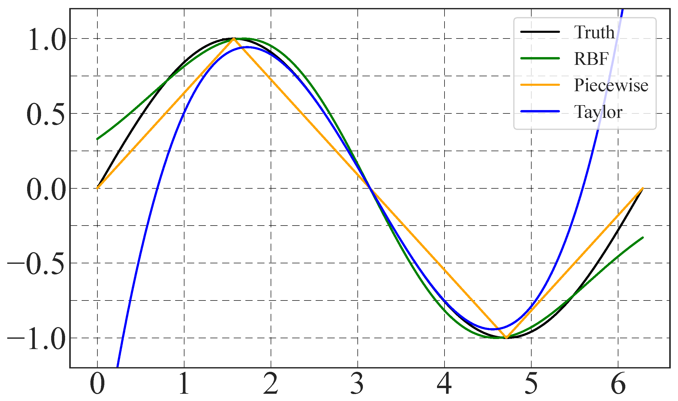
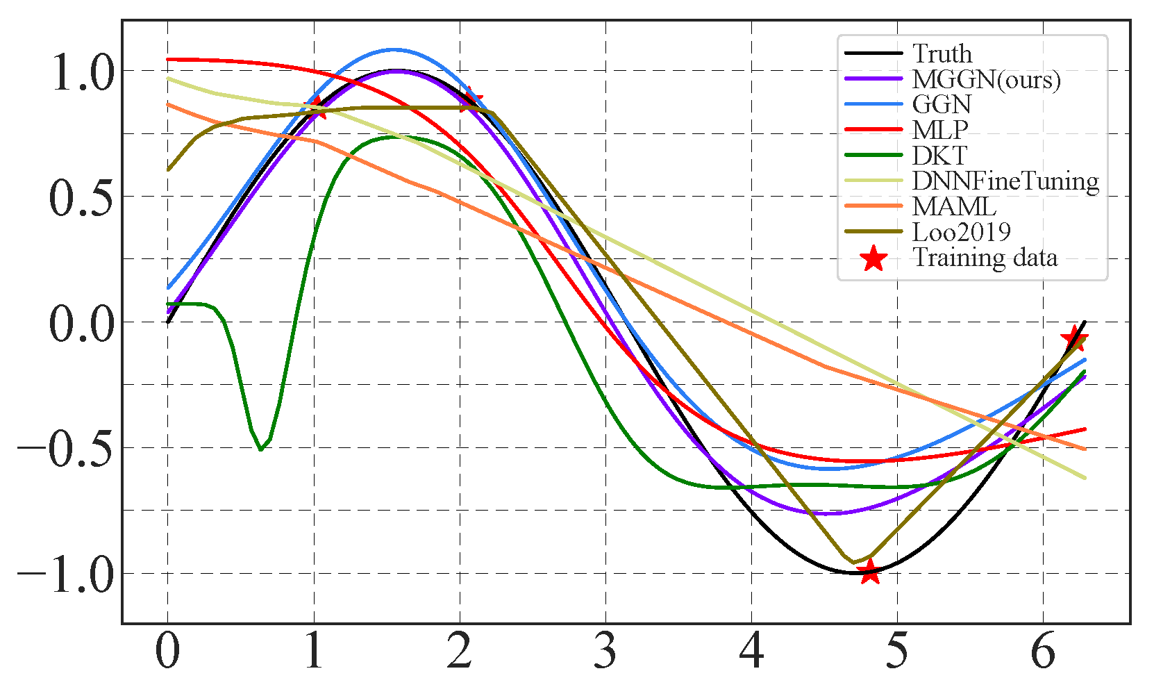
4.1. Sine Regression

The sine regression task targets the function shown in Equation (14):

$$f\left(x\right)=sin\left(x\right),x\in [0,2\pi ].$$

(14)

Figure 5 shows three complementary reference models: Piecewise, Radial Basis Function (RBF), and Taylor expansion models. Each model excels in different regions: the Piecewise model captures global trends robustly, the RBF model handles local variations effectively, and the Taylor model provides high accuracy near the expansion point.

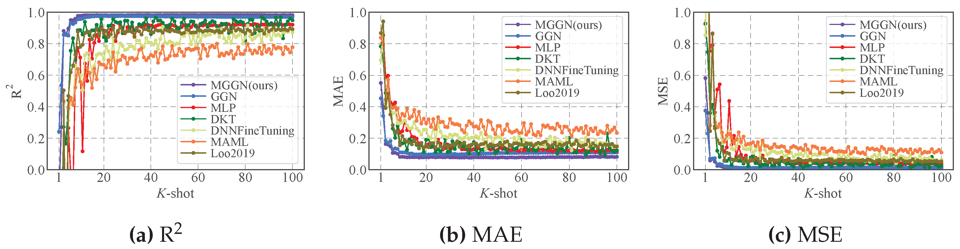
4.2. Results Comparison

We assessed model performance across various sample sizes (K-shot) using multiple metrics (R², MAE, MSE). MGGN incorporates Piecewise, Taylor, and RBF reference models, while GGN uses only the Piecewise model. Figure 6 and

Table 1. MAE ± standard deviation for the sine regression task under few-shot scenarios ($K\le 10$). Bold values represent optimal results.

K	MGGN (Ours)	GGN	MLP	DKT	DNNFineTuning	MAML	Loo2019
1	0.551 ± 0.253	0.454 ± 0.194	0.784 ± 0.121	0.784 ± 0.123	0.696 ± 0.274	0.838 ± 0.610	0.868 ± 0.311
2	0.406 ± 0.233	0.342 ± 0.150	0.854 ± 0.302	0.699 ± 0.106	0.873 ± 0.489	0.798 ± 0.562	0.942 ± 0.587
3	0.163 ± 0.040	0.185 ± 0.038	0.590 ± 0.162	0.488 ± 0.082	0.419 ± 0.062	0.445 ± 0.059	0.392 ± 0.074
4	0.160 ± 0.051	0.170 ± 0.041	0.598 ± 0.263	0.479 ± 0.187	0.533 ± 0.362	0.572 ± 0.446	0.484 ± 0.505
5	0.149 ± 0.045	0.183 ± 0.053	0.428 ± 0.116	0.414 ± 0.145	0.395 ± 0.063	0.405 ± 0.078	0.351 ± 0.108
6	0.107 ± 0.019	0.129 ± 0.020	0.416 ± 0.238	0.262 ± 0.081	0.361 ± 0.039	0.393 ± 0.056	0.283 ± 0.074
7	0.108 ± 0.025	0.136 ± 0.022	0.427 ± 0.207	0.203 ± 0.043	0.362 ± 0.073	0.400 ± 0.049	0.243 ± 0.071
8	0.102 ± 0.041	0.132 ± 0.037	0.291 ± 0.114	0.277 ± 0.131	0.296 ± 0.092	0.389 ± 0.084	0.241 ± 0.113
9	0.082 ± 0.008	0.111 ± 0.019	0.236 ± 0.082	0.174 ± 0.053	0.295 ± 0.057	0.317 ± 0.049	0.156 ± 0.057
10	0.083 ± 0.007	0.110 ± 0.013	0.245 ± 0.093	0.167 ± 0.048	0.301 ± 0.078	0.355 ± 0.068	0.215 ± 0.037

show MGGN consistently achieves superior performance across all metrics. For $K>10$, R² remains consistently high while MAE and MSE demonstrate rapid convergence with reduced variability compared to other methods.

Figure 7 demonstrates regression results for $K=4$, displaying the true function alongside predictions from MGGN and six comparative methods. MGGN better preserves the underlying sine function structure in sparse data regions, maintaining periodicity and smoothness. The MGGN predicted curve shows greater continuity with interpolated values closely matching ground truth.

4.3. Reference Model Combination Analysis

We analyzed the impact of different reference model combinations on MGGN and GGN performance in sine regression. Since single-reference performance characteristics were similar for both methods, only GGN results with individual reference models are reported.

Table 2. MAE ± standard deviation for the sine regression task under few-shot scenarios for various reference model combinations ($K\le 10$). Bold values represent optimal results.

K	MGGN (Ours)				GGN
	PRT	PR	PT	RT	P	R	T
1	0.551 ± 0.253	0.477 ± 0.193	0.533 ± 0.224	0.800 ± 0.236	0.454 ± 0.194	0.388 ± 0.144	1.237 ± 0.156
2	0.406 ± 0.233	0.267 ± 0.059	0.344 ± 0.297	0.356 ± 0.338	0.342 ± 0.150	0.269 ± 0.103	0.853 ± 0.444
3	0.163 ± 0.040	0.282 ± 0.159	0.235 ± 0.103	0.379 ± 0.352	0.185 ± 0.038	0.204 ± 0.037	0.370 ± 0.110
4	0.160 ± 0.051	0.217 ± 0.066	0.171 ± 0.057	0.168 ± 0.057	0.170 ± 0.041	0.167 ± 0.027	0.326 ± 0.211
5	0.149 ± 0.045	0.162 ± 0.031	0.116 ± 0.036	0.153 ± 0.043	0.183 ± 0.053	0.164 ± 0.033	0.266 ± 0.060
6	0.107 ± 0.019	0.134 ± 0.023	0.102 ± 0.027	0.160 ± 0.030	0.129 ± 0.020	0.132 ± 0.018	0.283 ± 0.066
7	0.108 ± 0.025	0.140 ± 0.023	0.100 ± 0.023	0.138 ± 0.024	0.136 ± 0.022	0.130 ± 0.024	0.282 ± 0.062
8	0.102 ± 0.041	0.132 ± 0.015	0.103 ± 0.016	0.154 ± 0.021	0.132 ± 0.037	0.128 ± 0.015	0.299 ± 0.065
9	0.082 ± 0.008	0.118 ± 0.017	0.097 ± 0.007	0.170 ± 0.065	0.111 ± 0.019	0.115 ± 0.016	0.275 ± 0.044
10	0.083 ± 0.007	0.111 ± 0.017	0.106 ± 0.015	0.149 ± 0.014	0.110 ± 0.013	0.121 ± 0.017	0.308 ± 0.059

shows notable differences between MGGN multi-model configurations (PRT, PR, PT, and RT) and GGN single-model deployments (P, R, and T) across sample sizes.

P, R, and T represent Piecewise, RBF, and Taylor expansion models, respectively, with PR, PT, RT, and PRT indicating their combinations. Under extremely limited samples ($K=1$), the single RBF model yields relatively favorable results. However, for $K\ge 3$, multiple reference model benefits become evident, with the complete combination (PRT) consistently achieving optimal results, particularly for larger sample sizes ($K\ge 8$). Results indicate that combining complementary reference models significantly enhances regression model robustness and accuracy under Limited-Sample conditions. Multi-model fusion outperforms single-model strategies by effectively mitigating individual model limitations as training samples increase.

5. Conclusions

This study introduces the Multi-Gradient Guided Network (MGGN) for addressing Limited-Sample regression challenges, representing a significant advancement in leveraging theoretical knowledge for data-scarce learning scenarios. The framework makes several key contributions: demonstrating that multiple reference models provide complementary gradient information that can be effectively combined through our PCGrad-based conflict resolution mechanism, establishing an adaptive weighting strategy that balances contributions from different theoretical sources, and showing that coordinated guidance from multiple reference models consistently outperforms traditional single-model methodologies. Our approach successfully addresses the fundamental challenge of merging potentially conflicting gradient directions while preserving useful information from each reference model and mitigating destructive interference, enriching the optimization process with diverse gradient perspectives that enhance learning efficiency in data-scarce environments.

Experimental validation on sine regression demonstrates that MGGN achieves superior performance compared to representative baselines including meta-learning methods, attention-based approaches, and fine-tuning strategies across all evaluated metrics (R², MAE, and MSE). The method’s ability to maintain function structure and periodicity even with extremely limited training data highlights its practical value for real-world applications where data acquisition is costly or challenging. Future research directions include extending the methodology to multi-dimensional and complex real-world Limited-Sample regression applications, developing adaptive mechanisms for automatic reference model selection, and establishing comprehensive evaluation frameworks for robust assessment of regression performance under various data scarcity conditions.

References

1. Zhang, D.; Liu, Z.; Jia, W.; Liu, H.; Tan, J. Contrastive Decoder Generator for Few-Shot Learning in Product Quality Prediction. IEEE Trans. Ind. Inform. 2022, 19, 11367–11379. [Google Scholar] [CrossRef]
2. Ahuja, C.; Sethia, D. Harnessing Few-Shot Learning for EEG signal classification: A survey of state-of-the-art techniques and future directions. Front. Hum. Neurosci. 2024, 18, 1421922. [Google Scholar] [CrossRef] [PubMed]
3. Yang, M.; Yang, Q.; Shao, J.; Wang, G. Runoff Prediction in a Data Scarce Region Based on Few-Shot Learning. In Proceedings of the IGARSS 2022-2022 IEEE International Geoscience and Remote Sensing Symposium, Kuala Lumpur, Malaysia, 17–22 July 2022; pp. 6304–6307. [Google Scholar]
4. Wang, Y.; Yao, Q.; Kwok, J.T.; Ni, L.M. Generalizing from a few examples: A survey on few-shot learning. ACM Comput. Surv. 2020, 53, 1–34. [Google Scholar] [CrossRef]
5. Snell, J.; Swersky, K.; Zemel, R. Prototypical networks for few-shot learning. Adv. Neural Inf. Process. Syst. 2017, 30. [Google Scholar] [CrossRef]
6. Vinyals, O.; Blundell, C.; Lillicrap, T.; Wierstra, D. Matching networks for one shot learning. Adv. Neural Inf. Process. Syst. 2016, 29. [Google Scholar] [CrossRef]
7. Yosinski, J.; Clune, J.; Bengio, Y.; Lipson, H. How transferable are features in deep neural networks? Adv. Neural Inf. Process. Syst. 2014, 27. [Google Scholar] [CrossRef]
8. Qi, H.; Brown, M.; Lowe, D.G. Low-shot learning with imprinted weights. In Proceedings of the IEEE Conference on Computer Vision and Pattern Recognition, Salt Lake City, UT, USA, 18–22 June 2018; pp. 5822–5830. [Google Scholar]
9. Li, Z.; Zhou, F.; Chen, F.; Li, H. Meta-sgd: Learning to learn quickly for few-shot learning. arXiv 2017, arXiv:1707.09835. [Google Scholar]
10. Sung, F.; Yang, Y.; Zhang, L.; Xiang, T.; Torr, P.H.S.; Hospedales, T.M. Learning to compare: Relation network for few-shot learning. In Proceedings of the IEEE Conference on Computer Vision and Pattern Recognition, Salt Lake City, UT, USA, 18–22 June 2018; pp. 1199–1208. [Google Scholar]
11. Tipton, E. Small sample adjustments for robust variance estimation with meta-regression. Psychol. Methods 2015, 20, 375. [Google Scholar] [CrossRef] [PubMed]
12. Chen, Y.; Liu, Z.; Xu, H.; Darrell, T.; Wang, X. Meta-baseline: Exploring simple meta-learning for few-shot learning. In Proceedings of the IEEE/CVF International Conference on Computer Vision, Montreal, BC, Canada, 11–17 October 2021; pp. 9062–9071. [Google Scholar]
13. Chao, X.; Zhang, L. Few-shot imbalanced classification based on data augmentation. Multimed. Syst. 2023, 29, 2843–2851. [Google Scholar] [CrossRef]
14. Shi, P.; Huang, G.; He, H.; Zhao, G.; Hao, X.; Huang, Y. Few-shot regression with differentiable reference model. Inf. Sci. 2024, 658, 120010. [Google Scholar] [CrossRef]
15. Yu, T.; Kumar, S.; Gupta, A.; Levine, S.; Hausman, K.; Finn, C. Gradient surgery for multi-task learning. Adv. Neural Inf. Process. Syst. 2020, 33, 5824–5836. [Google Scholar]
16. Tang, M.; Jin, Z.; Zou, L.; Shiuan-Ni, L. Learning to Resolve Conflicts in Multi-Task Learning. In Proceedings of the International Conference on Artificial Neural Networks, Crete, Greece, 26–29 September 2023; pp. 477–489. [Google Scholar]
17. Sener, O.; Koltun, V. Multi-task learning as multi-objective optimization. Adv. Neural Inf. Process. Syst. 2018, 31. [Google Scholar] [CrossRef]
18. Patacchiola, M.; Turner, J.; Crowley, E.J.; O’Boyle, M.; Storkey, A.J. Bayesian meta-learning for the few-shot setting via deep kernels. Adv. Neural Inf. Process. Syst. 2020, 33, 16108–16118. [Google Scholar]
19. Loo, Y.; Lim, S.K.; Roig, G.; Cheung, N.M. Few-shot regression via learned basis functions. Int. Conf. Learn. Represent. 2019. Available online: https://openreview.net/forum?id=r1ldYi9rOV (accessed on 15 June 2025).
20. Finn, C.; Abbeel, P.; Levine, S. Model-agnostic meta-learning for fast adaptation of deep networks. In Proceedings of the International Conference on Machine Learning, Sydney, Australia, 6–11 August 2017; pp. 1126–1135. [Google Scholar]
21. Zeng, W.; Xiao, Z.Y. Few-shot learning based on deep learning: A survey. Math. Biosci. Eng. 2024, 21, 679–711. [Google Scholar] [CrossRef] [PubMed]
22. Baik, S.; Choi, M.; Choi, J.; Kim, H.; Lee, K.M. Learning to learn task-adaptive hyperparameters for few-shot learning. IEEE Trans. Pattern Anal. Mach. Intell. 2023, 46, 1441–1454. [Google Scholar] [CrossRef] [PubMed]
23. Savaşlı, Ç.; Tütüncü, D.; Ndigande, A.P.; Özer, S. Performance analysis of meta-learning based bayesian deep kernel transfer methods for regression tasks. In Proceedings of the 2023 31st Signal Processing and Communications Applications Conference (SIU), Istanbul, Turkey, 5–8 July 2023; pp. 1–4. [Google Scholar]
24. Oreshkin, B.; Rodríguez López, P.; Lacoste, A. Tadam: Task dependent adaptive metric for improved few-shot learning. Adv. Neural Inf. Process. Syst. 2018, 31. [Google Scholar] [CrossRef]
25. Sui, X.; He, S.; Zheng, Y.; Che, Y.; Teodorescu, R. Early Prediction of Lithium-Ion Batteries Lifetime via Few-Shot Learning. In Proceedings of the IECON 2023-49th Annual Conference of the IEEE Industrial Electronics Society, Singapore, 16–19 October 2023; pp. 1–6. [Google Scholar]
26. Xu, J.; Li, K.; Li, D. An Automated Few-Shot Learning for Time Series Forecasting in Smart Grid Under Data Scarcity. IEEE Trans. Artif. Intell. 2024, 6, 2482–2492. [Google Scholar] [CrossRef]
27. Hou, H.; Bi, S.; Zheng, L.; Lin, X.; Quan, Z. Sample-efficient cross-domain WiFi indoor crowd counting via few-shot learning. In Proceedings of the 2022 31st Wireless and Optical Communications Conference (WOCC), Shenzhen, China, 11–12 August 2022; pp. 132–137. [Google Scholar]
28. Chen, X.; Yi, J.; Wang, A.; Deng, X. Wi-Fi Fingerprint Based Indoor Localization Using Few Shot Regression. EasyChair Preprint 2024. [Google Scholar] [CrossRef]
29. Tian, P.; Xie, S. An adversarial meta-training framework for cross-domain few-shot learning. IEEE Trans. Multimed. 2022, 25, 6881–6891. [Google Scholar] [CrossRef]
30. Lim, J.Y.; Lim, K.M.; Lee, C.P.; Tan, Y.X. SSL-ProtoNet: Self-supervised Learning Prototypical Networks for few-shot learning. Expert Syst. Appl. 2024, 238, 122173. [Google Scholar] [CrossRef]
Figure 1. Optimization trajectories contrasting single- and multi-gradient training strategies. The visualization demonstrates how multi-gradient guidance (red dashed trajectory) achieves more direct convergence from the initial point to the optimal solution compared to single-gradient approaches (blue dashed trajectory), which shows more circuitous paths and potential convergence to suboptimal points (O1 vs. O2). The gradient vectors G1, G2, and G3 represent different reference model gradients that are fused to provide more robust optimization directions, ultimately leading to better alignment with the ground truth and faster convergence in the parameter space.
Information 16 00619 g001
Figure 2. Gradient-guided network approach for Limited-Sample regression. The framework illustrates how theoretical reference model gradients (black arrows) are incorporated as training constraints to guide the neural network learning process, where gradient sampling points provide additional supervision beyond the limited training samples (red dots). The Truth function (blue solid line) and network prediction (purple dashed line) demonstrate the effectiveness of gradient guidance in maintaining function structure even with sparse data.
Information 16 00619 g002
Figure 3. Multi-gradient fusion: (a) Detecting gradient conflicts via inner product sign; (b) applying orthogonal projection to conflicting gradients; (c) weighted merging based on sample coverage.
Information 16 00619 g003
Figure 4. The framework of MGGN. The architecture shows the complete pipeline from multiple reference models through gradient fusion to final network training: (a) Input Module with training data and reference models g1(x), g2(x), g3(x); (b) neural network with sigmoid activation; (c) gradient fusion using PCGrad with adaptive weighting; (d) Loss Computation combining prediction and gradient losses; (e) Output Module comparing predictions with ground truth, highlighting the key innovation of multi-gradient integration compared to traditional single-gradient approaches.
Information 16 00619 g004
Figure 5. Comparison between the sine regression target function and reference models: truth (black), Taylor (blue), RBF (green), and Piecewise (orange). The figure illustrates how different reference models approximate the target sine function across the input domain.
Information 16 00619 g005
Figure 6. Model performance comparison with varying training sample numbers.
Information 16 00619 g006
Figure 7. Regression performance comparison for K = 4 .
Information 16 00619 g007