Efficient Hotspot Detection in Solar Panels via Computer Vision and Machine Learning

Abstract

Solar power generation is rapidly emerging within renewable energy due to its cost-effectiveness and ease of deployment. However, improper inspection and maintenance lead to significant damage from unnoticed solar hotspots. Even with inspections, factors like shadows, dust, and shading cause localized heat, mimicking hotspot behavior. This study emphasizes interpretability and efficiency, identifying key predictive features through feature-level and What-if Analysis. It evaluates model training and inference times to assess effectiveness in resource-limited environments, aiming to balance accuracy, generalization, and efficiency. Using Unmanned Aerial Vehicle (UAV)-acquired thermal images from five datasets, the study compares five Machine Learning (ML) models and five Deep Learning (DL) models. Explainable AI (XAI) techniques guide the analysis, with a particular focus on MPEG (Moving Picture Experts Group)-7 features for hotspot discrimination, supported by statistical validation. Medium Gaussian SVM achieved the best trade-off, with 99.3% accuracy and 18 s inference time. Feature analysis revealed blue chrominance as a strong early indicator of hotspot detection. Statistical validation across datasets confirmed the discriminative strength of MPEG-7 features. This study revisits the assumption that DL models are inherently superior, presenting an interpretable alternative for hotspot detection; highlighting the potential impact of domain mismatch. Model-level insight shows that both absolute and relative temperature variations are important in solar panel inspections. The relative decrease in “blueness” provides a crucial early indication of faults, especially in low-contrast thermal images where distinguishing normal warm areas from actual hotspot is difficult. Feature-level insight highlights how subtle changes in color composition, particularly reductions in blue components, serve as early indicators of developing anomalies.

1. Introduction

The United Nations Sustainable Development Goals (SDGs), especially the seventh goal, emphasize the significance of affordable, reliable, sustainable, and modern energy for all. In this context, solar energy is attracting attention due to its environmental benefits and economic potential. The key driver for this renewable energy technology is the solar cell that converts sunlight to electricity. However, the widespread adoption of solar energy presents challenges, such as the occurrence of hotspots. Hotspots are localized areas on solar panels that experience significantly higher temperatures than the surrounding areas, leading to reduced power loss of 25% [1] and potential fire damage. Figure 1 illustrates the thermal images of healthy and defective PV panels with hotspots. Addressing hotspot faults is critical to ensure the long-term performance and reliability of solar power systems. Neglecting these issues results in premature degradation, power output losses, and even safety hazards, ultimately impacting the economic viability and environmental sustainability of solar energy. It is shown in industry reports that there is a rapid rise in Asia Pacific solar power market size, and it is expected to be worth USD 178.24 billion by 2034 [2]. Furthermore, it is highlighted that PV incentive policies, such as the Sunshine Program, the PV Roadmap toward 2030, and initiatives focused on advancing next-generation solar cells, were overseen by the Ministry of Education, Culture, Sports, Science, and Technology (MEXT) and actively promoted by the Japan Science and Technology Agency (JST) [3]. The de facto principle is that solar powered electricity generation dominates the world energy market. If hotspots are not identified at early stages, with the effect of internal and external factors, the severity will becoming higher, the panel efficiency will drop, and the panel will be damaged. And if this persists further, it could result in a fire hazard. This is a red alarm for the safety of the system.

Despite recent advances in thermal image analysis, several critical research gaps remain unaddressed. One major limitation is the lack of computational efficiency analysis, as most existing studies emphasize classification accuracy while overlooking computational efficiency analysis. Training and inference times are rarely reported, although they are essential for deployment in resource-constrained environments such as Unmanned Aerial Vehicles (UAVs) [5,6]. Another significant limitation is that traditional Machine Learning (ML) approaches using handcrafted features such as histograms of oriented gradients and texture lack interpretability mechanisms and provide no explanation for the predictions of the model. A further critical challenge lies in the high hardware cost and limited scalability of sensor-dependent methods, which, despite achieving high accuracy, rely on additional electrical measurements, thus increasing system complexity and limiting large-scale aerial inspections. Furthermore, domain mismatch in deep models is another significant limitation. Deep Learning (DL) models based on transfer learning from convolutional neural networks pre-trained on RGB ImageNet (i.e., natural images composed of red, green, and blue color channels, representing how standard cameras capture visual scenes) often perform poorly when applied to IR thermal imagery due to domain mismatch, with models like VGG-16 achieving around 68% accuracy. However, no domain-adaptation strategies have been explored to address this issue. Lastly, there is no unified benchmarking framework that jointly evaluates classification performance, computational cost, and interpretability using explainable artificial intelligence tools such as SHAP (SHapley Additive exPlanations) and What-if Analysis. These limitations highlight the need for a comprehensive approach to thermal image classification that considers real-world constraints.

This research contributes to the literature in four key areas.

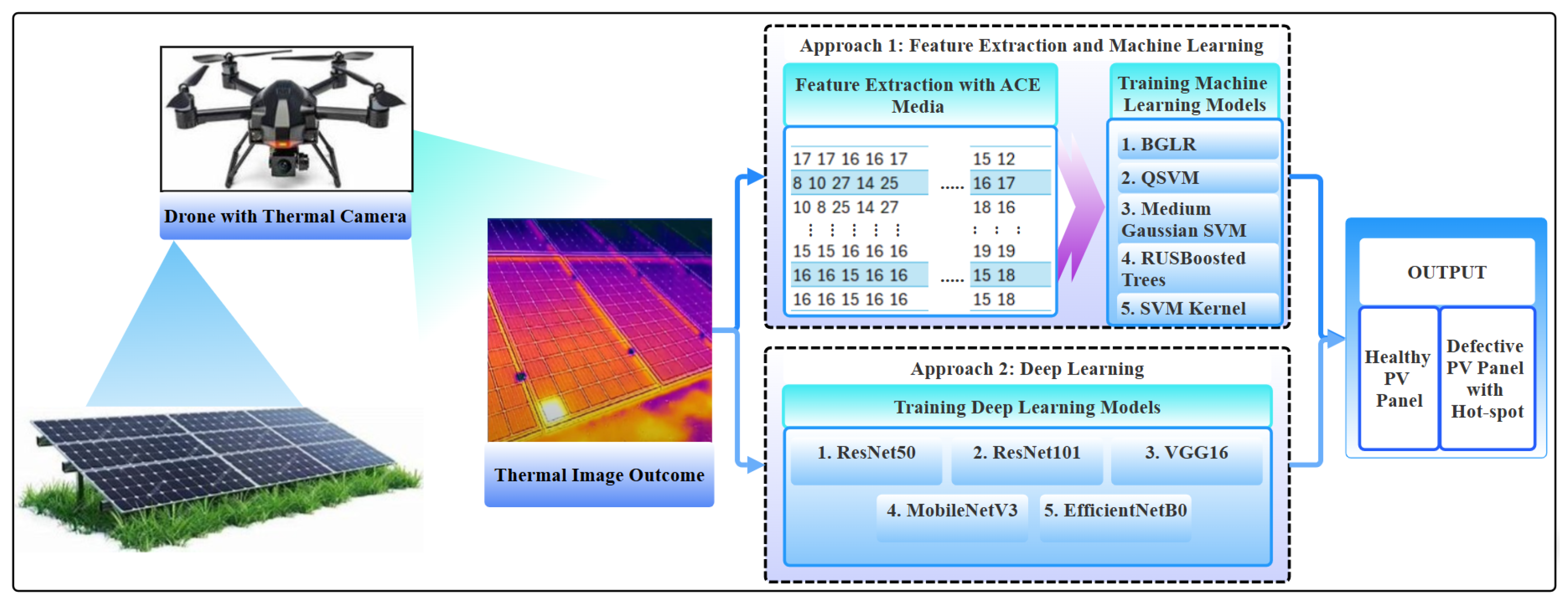
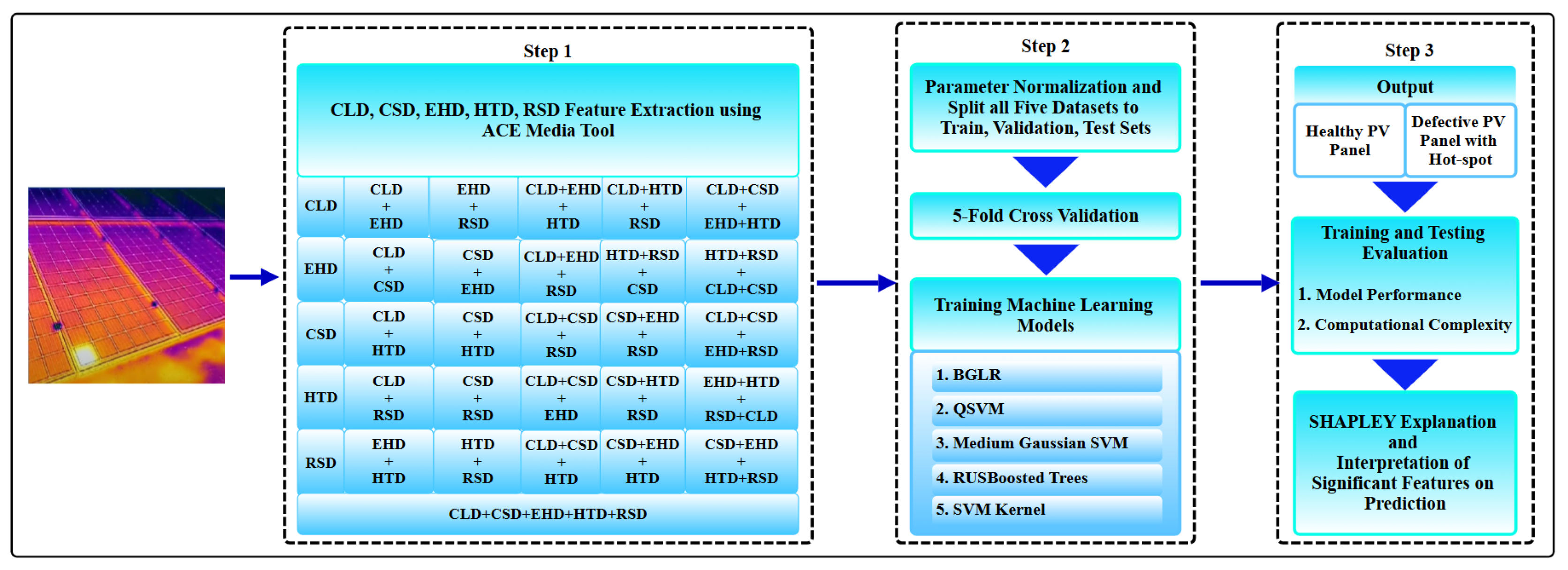
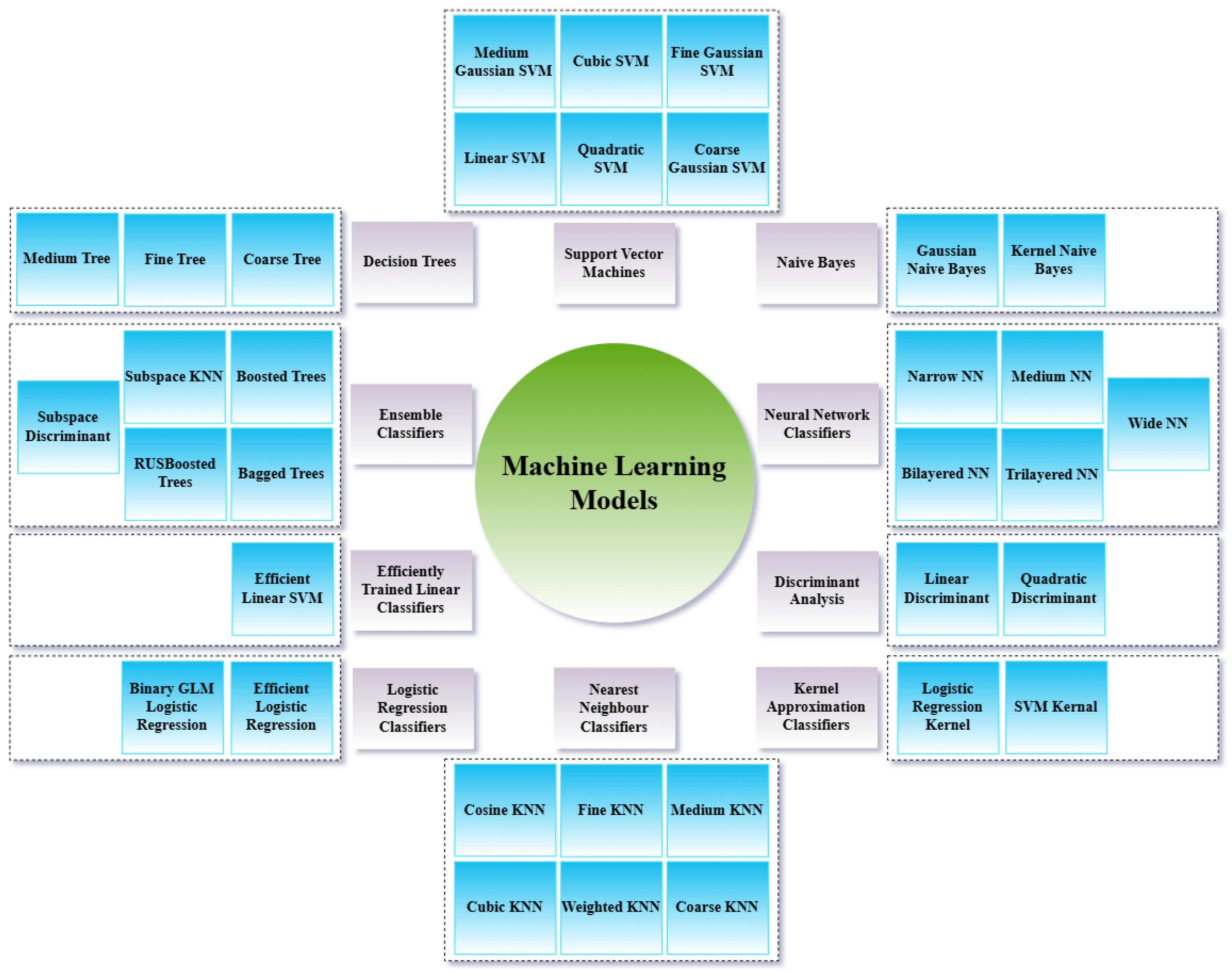
• The first is to evaluate 34 ML vs. 5 leading DL models. The study adopts a global approach, covering 34 ML models for 31 feature combinations. The feature extraction is carried out by the Automatic Content Extraction (ACE) media tool in ML models for five different datasets containing thermal images of solar panels with hotspots. The existing literature has predominantly focused on DL models and electrical parameter measurement of solar panel power generation.
• The second objective is to assess Explainable AI (XAI) interpretability via SHAP and What-if Analysis. The study employs a novel methodology that combines SHAP and What-if Analysis [7,8]. This enhances the interpretability of ML models, as part of the XAI [9] framework, in the context of (Unmanned Aerial Vehicle) UAV-based photovoltaic (PV) hotspot detection using thermal imagery. A novel methodology combining SHAP and What-if Analysis is employed to enhance the interpretability of ML models within the XAI framework, specifically for (Unmanned Aerial Vehicle) UAV-based photovoltaic (PV) hotspot detection using thermal imagery. This approach examines the linkage between the performance and computational complexity of both ML and DL models for this application. It highlights that feature-extraction-based ML models outperform DL models. In particular, transfer-learning-based CNNs trained on the ImageNet database lack effective generalization for domain-specific tasks like infrared-based solar panel hotspot detection [10,11].
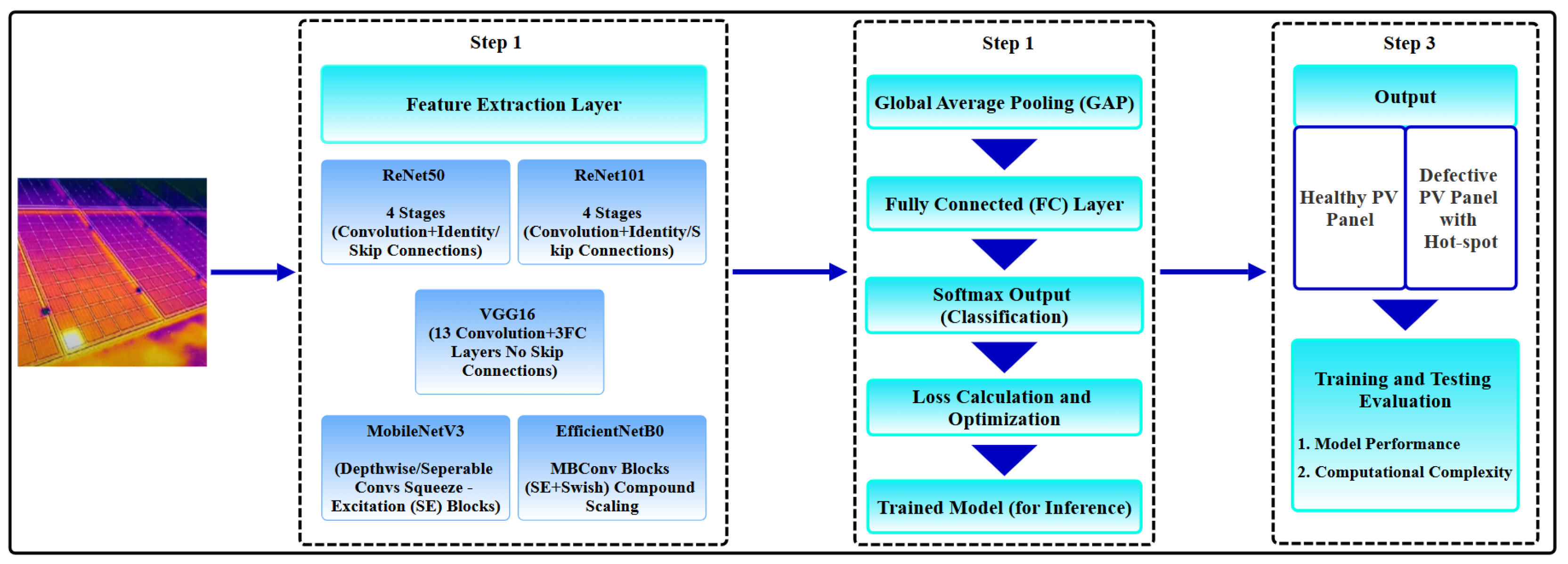
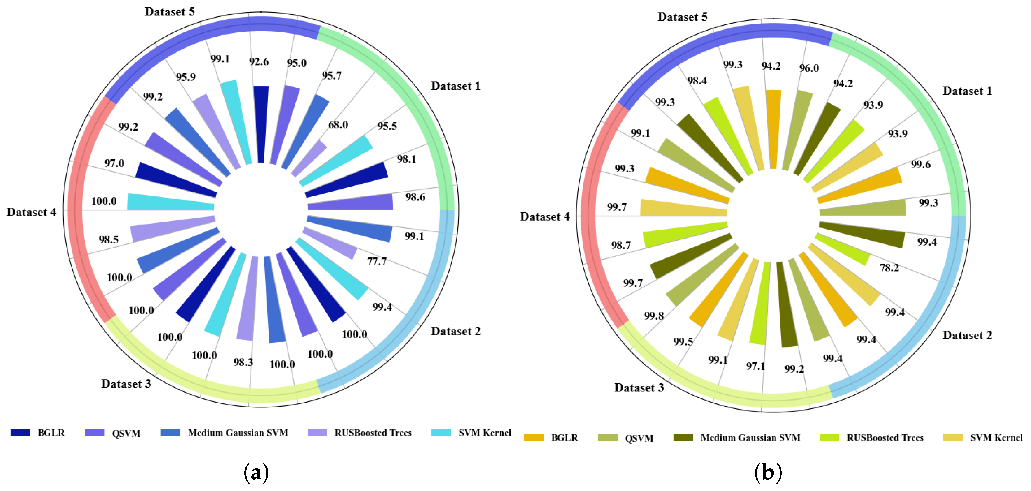
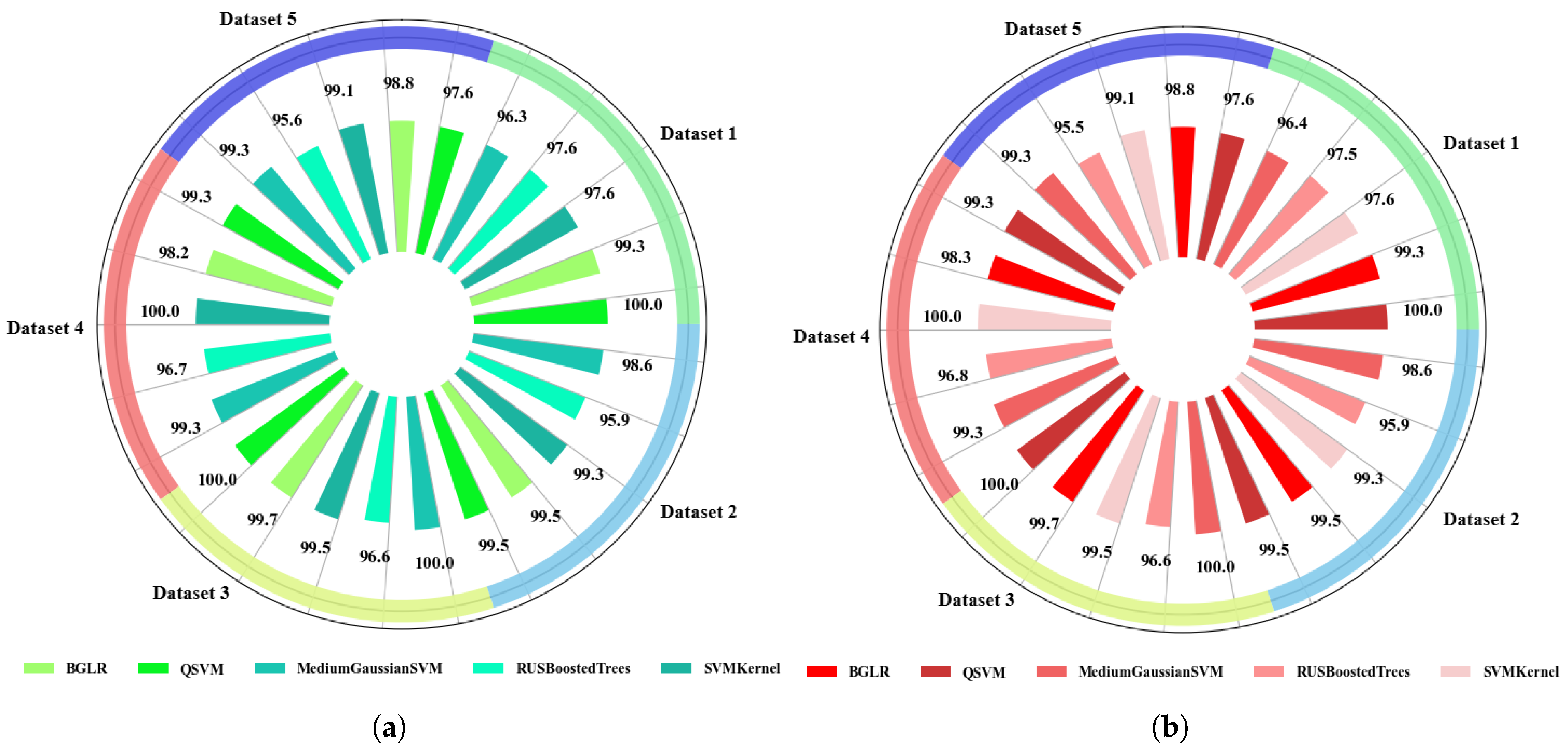
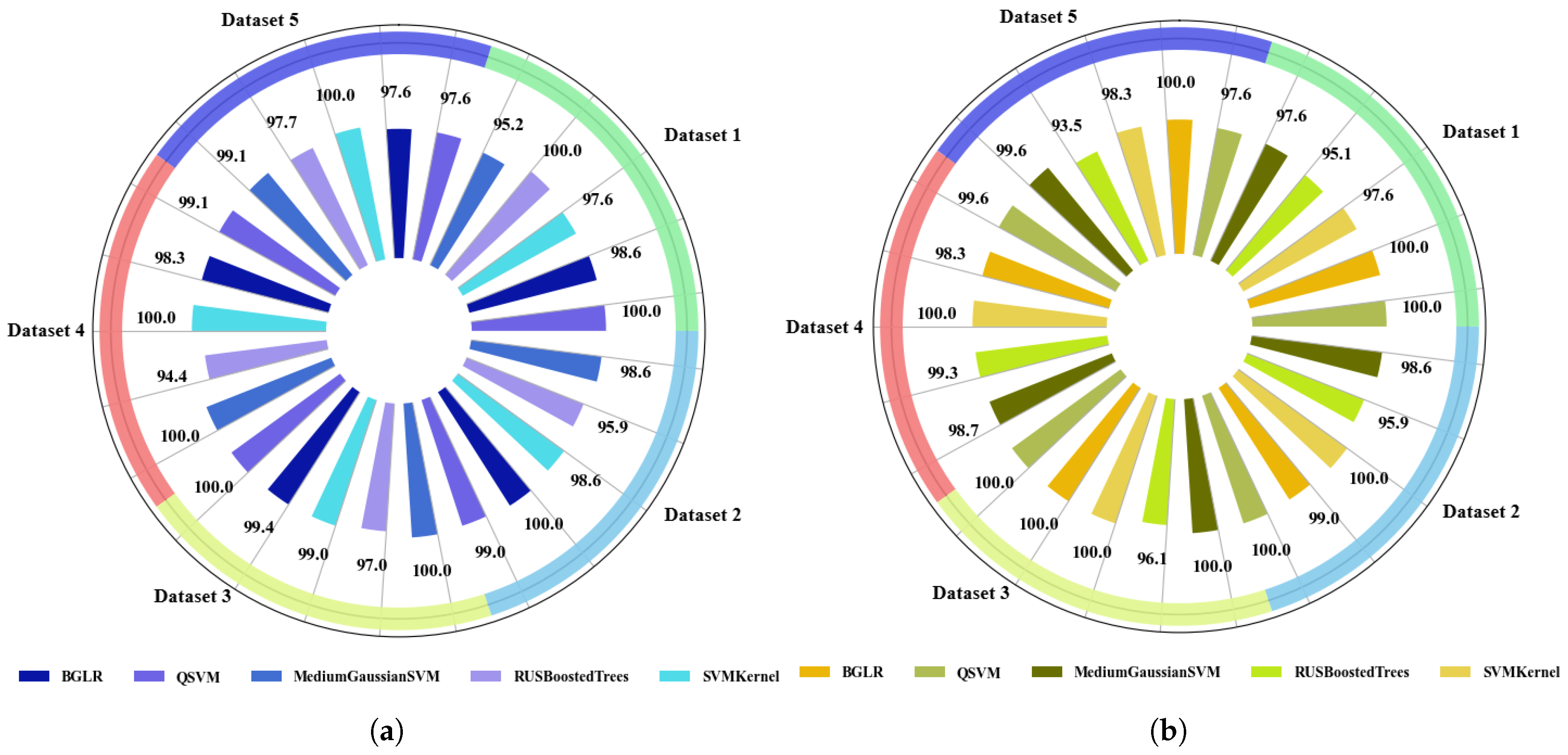
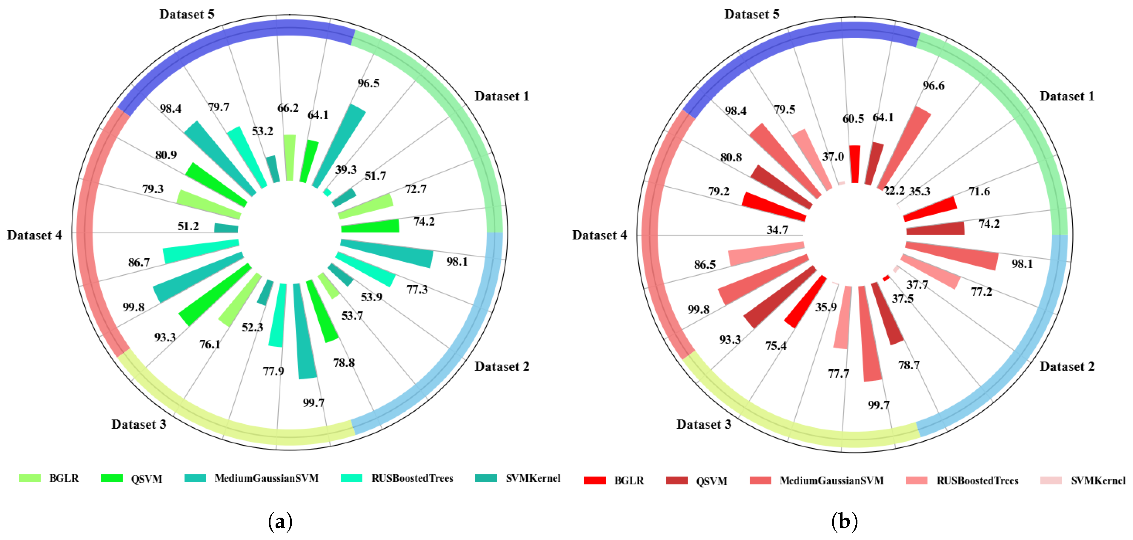
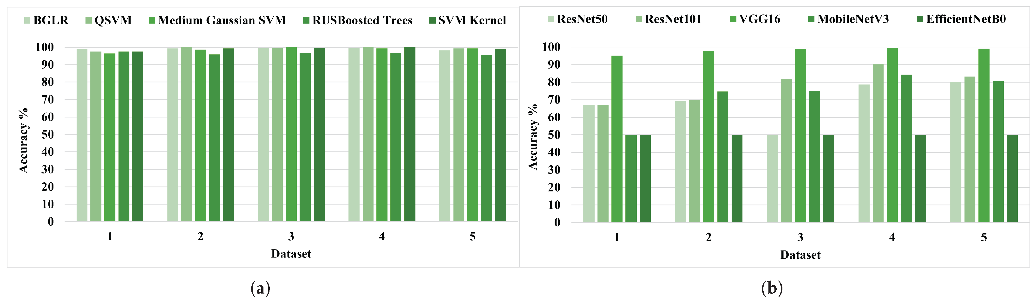
• The third is to evaluate the classification performance and computational efficiency of the top five ML and DL models: It provides comprehensive insights by plotting and summarizing accuracy and time-scale graphs. These graphs are based on five datasets. The analysis includes the top five high-performing ML models, which are Binary GLM Logistic Regression, Quadratic Support Vector Machine, Medium Gaussian Support Vector Machine, RUSBoosted Trees, and Support Vector Machine Kernel. In addition, five DL models are also considered: ResNet-50, ResNet-101, VGG-16, MobileNetV3Small, and EfficientNetB0. Further, the computational efficiency is analyzed, with an emphasis on training and inference times, to determine the feasibility of deployment in resource-constrained environments.
• The final objective is to synthesize and recommend the optimum performing ML model suitable for UAV deployment: Research identifies optimal models that ensure a balance between predictive accuracy, generalization across datasets, and computational resource requirements, thus supporting practical and scalable real-world deployment.

Roadmap of the study.

To support the four research objectives, the manuscript has been carefully structured to ensure logical flow, clarity, and coherence. It begins with a focused literature review, covering thermal image-based feature extraction, ML and DL-based approaches for solar PV hotspot detection, and the limitations of existing methods. This is followed by a section on the significance of the study, which highlights key research gaps. The methodology presents a dual-approach framework: (1) traditional ML pipelines incorporating MPEG (Moving Picture Experts Group)-7 feature extraction and benchmarking of 34 models, and (2) end-to-end DL modeling using five state-of-the-art architectures, both complemented by XAI techniques such as SHAP and What-if Analysis. The results section presents detailed analyses of classification accuracy and computational efficiency (training and testing time) across five datasets, followed by a comparative discussion. The discussion provides local and global model interpretability using XAI methods and offers a comparative evaluation between ML and DL models, including statistical validation. A dedicated section explores the trade-offs between accuracy and resource utilization, reinforcing the practical implications of the findings. Finally, the paper concludes with recommendations for UAV-based deployment, highlighting optimal model choices and future research directions. This structured layout cohesively integrates the diverse components of the study, enhancing readability and guiding the reader clearly through each phase of the investigation.

2. Literature Review

This section provides a focused thematic review of recent methodological works including both classical ML and modern DL approaches applied to UAV-based solar PV hotspot detection. Rather than a generic review, it critically evaluates how these studies perform with respect to model accuracy, feature extraction, and operational constraints like computational efficiency and interpretability.

While many studies achieve high performance on standard metrics such as Accuracy, Precision, Recall, and F1-score, they frequently overlook essential deployment-focused indicators such as training time, inference time, and cross-dataset generalization. This gap limits the practical viability of their methods for real-world, resource-constrained PV monitoring systems.

To highlight the novelty and relevance of our proposed work, we organize this review into four focused sub-sections: a study on thermal image-based feature extraction techniques, a review of classical ML-based approaches, a discussion of DL-based techniques, and a concluding sub-section evaluating the significance of these methods in the context of UAV-assisted solar PV hotspot detection. Each sub-section identifies key limitations in previous studies that this work aims to address, especially regarding interpretability, computational efficiency, and deployment readiness.

2.1. Study on Thermal Image-Based Feature Extraction for Solar PV Hotspot Detection

Although the study [12] investigates the Histogram of Oriented Gradient (HOG) and texture features and reports an accuracy of 73.8%; the performance can potentially be improved by incorporating additional features. While high-dimensional feature vectors are often considered challenging, in the domain-specific context of thermal image-based hotspot detection, they can be particularly beneficial. The rich, detailed features help capture subtle thermal variations, indicating that combining more feature types could further enhance model performance in this specialized application.

However, based on the studies [13,14], it is further revealed that although the accuracies are analyzed based on feature extraction, neither an evaluation of computational complexity nor an explicit interpretation of its predictions has been provided, which should be a must and an essential output in research findings for further deployment in UAV-assisted solar PV hotspot detection.

2.2. Investigation of ML-Based Techniques for Solar PV Hotspot Detection

The studies [15], which employed ML, achieved high accuracies. However, the electrical parameters were measured with sensors. To elaborate, the research [15] delves into the field of study with four classifiers, Decision Tree (DT), Support Vector Machine (SVM), K-Nearest Neighbor (KNN), and Discriminant Classifier (DC), with 15 classification algorithms with three different setups to analyze. Setup 1 utilized only the maximum power point $P_{\mathrm{mpp}}$ as input data, while setup 2 incorporated two parameters, $P_{\mathrm{mpp}}$ and $I_{\mathrm{sc}}$. Setup 3 expanded the input dataset to include three parameters, $P_{\mathrm{mpp}}$, $I_{\mathrm{sc}}$, and $V_{\mathrm{oc}}$. Each classifier was trained and evaluated across these setups to assess the impact of different input parameter combinations on classification performance, where DT achieved the lowest accuracy at 84% and DC reached the highest accuracy at 98%. To provide further insight, ref. [14] deployed SVM and the Feed-forward Back-Propagation Neural Network with 99% and 87% average accuracy, respectively, which required six input parameters, percentage power loss, open circuit voltage, short circuit current, irradiance, temperature, and impedance, for microcrack and hotspot classification in solar PV.

However, the accuracy and reliability of such sensor-based approaches are heavily dependent on the Precision of the measuring instruments. Scaling these methods for large solar farms demands a substantial number of additional sensors, which significantly increases costs related to hardware, installation, maintenance, compatibility, and the need for skilled personnel. While these methods may achieve high accuracy, they are often limited by their intrusive nature and lack of scalability. In contrast, the approach presented in this study addresses these limitations utilizing thermal imaging; a non-intrusive and non-contact technique that enables remote and real-time fault detection [16]. Furthermore, by integrating UAV-based deployment, the proposed method offers improved scalability and mobility.

2.3. Analysis of DL-Based Techniques for Solar PV Hotspot Detection

The research [17] investigates the pre-trained models designed and trained on the ImageNet [18,19] dataset, providing lower accuracies when using the transfer leaning [20] technique for the infrared (IR) image dataset. The reason is that the pre-trained models were trained on RGB (red–green–blue) images, illustrating a great difference in the physical characteristics with the thermal images. However, it is noted that only the parameters of the two added fully connected (FC) layers were updated since the parameters of the pre-trained models were frozen while training on the IR image dataset. This can be supported by the accuracy comparison study of different transfer learning models: VGG-16 achieves 68%, MobileNet reaches 57%, and ResNet-50 attains 69%.

To increase the accuracy, various techniques have been followed such as hybrid methods [21] and ensembles that combine different models and measurement of electrical parameters [22]. A hybrid scheme integrating three embedded learning models has been proposed for solar hotspot classification. The first mode, CNN (Convolutional Neural Network) Model 1, processes images using an improved gamma correction function for preprocessing. The second, CNN Model 2, utilizes IR temperature data from PV modules with a threshold function for preprocessing. The third, XGBoost Model 3, replaces CNN with the eXtreme Gradient Boosting (XGBoost) algorithm, leveraging selected temperature statistics. This hybrid approach achieves 93.8% accuracy in hotspot detection. An ensemble [17] achieves an accuracy of 86%. Nevertheless, Deep Neural Networks (DNNs) using the VGG-16 architecture with modified fully connected layers have been applied for thermal image classification, specifically for detecting hotspots and hot sub-strings [23]. Using the transfer learning technique, this approach achieves a classification accuracy of 98% [24]. The study [25] investigates the usage of an image dataset that deploys ResNet-50, which has an 85.37% harmonic mean of Precision and Recall. This performs two tasks in which the first model, ResNet-50, is the transfer learning model for the classification of the type of fault affecting the panel. Faster R-CNN identifies the region of interest of the faulty panel with a 67% mean average Precision. The edge image features of hotspots were extracted based on the Residual Neural Network (RNN), which is a DL architecture, for image segmentation by Mask R-CNN with 61.64% Precision [26]. In the study [22], the dataset of irradiance, temperature differences, and relative humidity, including thermal images, was used for the classification of whether a hotspot exists or not, while hotspot detection was carried out by random forest. However, these studies do not investigate computational complexity.

As illustrated in Figure 2, previous studies have predominantly focused on reporting accuracy [27,28,29] alone, while neglecting other critical performance indicators such as inference time, training time, and generalization ability across datasets. This limited scope restricts the depth of comparative analysis and impedes a comprehensive evaluation of model robustness and efficiency. The present study addresses this shortcoming by highlighting the importance of multi-metric evaluation and advocating for a more holistic framework in future research to enable meaningful and reliable comparisons.

Although the aforementioned DL models demonstrate commendable performance across specific tasks [30,31,32], they often present significant limitations [33] in terms of computational complexity, storage overhead, and interpretability. Many existing studies rely on large, resource-intensive architectures that are unsuitable for real-time UAV deployment scenarios, where lightweight, fast, and energy-efficient models are essential [13,34]. Furthermore, the “black-box” nature of DNN obscures the underlying decision-making process, reducing transparency and making it difficult to validate or interpret model outputs [35,36]. These gaps underscore the urgent need for robust and interpretable solutions tailored to the domain of solar hotspot detection. In this context, our study addresses these challenges by evaluating both traditional ML and DL models not only based on accuracy but also on training and testing time, generalizability across diverse datasets, and computational efficiency. This multi-metric framework enhances model selection for practical UAV-based applications and promotes explainability—an increasingly critical requirement for responsible AI deployment in energy and sustainability domains.

2.4. Review of Hotspot Detection Techniques in PV Systems

To ensure coherence with the review-based nature of this work, we summarize key review articles related to hotspot detection in PV systems. Ref. [37] presented a comprehensive review of existing hotspot mitigation strategies, comparing them in terms of cost, power loss, and temperature reduction. They also proposed a novel series-resistor-based circuit-level strategy, laying a foundation for practical implementations. The study [38] explored vision-based monitoring systems for PV fault detection, highlighting the role of image processing and AI techniques in identifying anomalies like hotspots, and discussed the scalability and limitations of such systems in large-scale solar farms. Additionally, ref. [39] focused on models for predicting PV cracks and hotspots, emphasizing the role of physical parameters such as microcrack orientation and propagation and underscoring the complexity in accurate long-term performance modeling. These review articles provide a broad understanding of both detection and mitigation efforts in PV systems. However, a gap remains in terms of real-time, hardware-implementable mitigation solutions. Our study addresses this gap by proposing an area-based evaluation framework. This positions our work as a bridge between theoretical mitigation concepts and potential real-time, UAV-deployable solutions.

2.5. Significance of the Study

In summary, although certain DL models offer considerably high accuracy in hotspot detection and classification, their complexity and lack of interpretability are some drawbacks that can be highlighted [33]. Classical ML models provide a complementary advantage by being computationally efficient and easier to understand, especially when combined with informative features. For real-world PV monitoring systems, a balanced approach that incorporates accuracy, efficiency, and explainability is critical for building robust and scalable solutions [14,15].

While prior studies have extensively reported conventional performance metrics such as Accuracy, Precision, Recall, and F1-score, they often lack a blended evaluation of these alongside deployment-critical metrics such as training time, inference time, and generalization ability across datasets. This study aims to fill that gap by adopting a comprehensive performance assessment strategy. In particular, the models were evaluated not only for their predictive performance but also for their efficiency and cross-dataset generalizability metrics that are vital for UAV-based PV monitoring applications where resource constraints and variability in input data are common.

Moreover, to our knowledge, no previous work has combined MPEG-7-based feature extraction with XAI techniques such as SHAP and a What-if Analysis framework in the context of UAV-assisted PV hotspot detection. By integrating these tools with traditional ML models, this study contributes a novel methodology that not only delivers high performance but also promotes interpretability, low computational complexity, and robust generalization. This positions the work as a meaningful contribution toward practical, explainable, and scalable fault detection in the solar energy domain.

3. Methodology

3.1. Background and Approach

This study focuses on integrating image processing on UAVs for hotspot detection in solar farms.

The aim is to perform an in-depth comparison and evaluation of the performance, resource utilization analysis and efficiency between two approaches, namely, approach 1, feature-extraction-based ML models, and, approach 2, transfer-learning-based Convolutional Neural Network (CNN) DL models. This section begins with an overview of the methodological framework, followed by the presentation of approach 1 and approach 2 in detail.

Approach 1 will discuss in detail the use of ML models based on procedures for extracting valuable image features and benchmarks for identifying top-performing ML algorithms. Subsequently, approach 2 will move towards DL approaches based on selected DL models with end-to-end neural network training without extracting features.

Figure 3 provides an overview of the study, and each component is discussed in detail in the subsequent sections.

(1)

Assess Selection of Solar Panel

According to Figure 3, images of monocrystalline solar panels have been captured by drone. Monocrystalline panels are widely installed at present due to higher energy conversion efficiency of within the 18–22% range compared to polycrystalline, which is lower in the 15–18% range. This type is more sensitive to hotspots, which cause more severe local heating and degradation in monocrystalline cells since they are often tightly packed for maximum efficiency. Hence, even a small hotspot quickly affects many cells. Further, this panel type is more expensive, so even a single hotspot damage causes greater financial losses if not detected early.

Monocrystalline solar panels from manufacturers such as SunPower (SunPower Corporation, San Jose, CA, USA) offering 400W; LG (LG Electronics Incorporated, Seoul, Republic of Korea) with 380W; Canadian Solar (Canadian Solar Incorporated, Guelph, ON, Canada) with 370W; JA Solar (JA Solar Technology Company Limited, Shanghai, China) with 370W; and Trina Solar (Trina Solar Limited, Changzhou, China) provide high efficiency and compact sizes and are widely used in both residential and commercial applications.

(2)

Thermal Data Acquisition using UAV and Dataset Preparation

Solar panels installed in large-scale solar farms are inspected using thermal cameras mounted on UAVs [40,41,42]. For small-scale solar installation, using handheld cameras would work, but when it comes to large-scale solar, this is not practical. Therefore, it is efficient and effective to use thermal cameras installed in UAV [43,44,45], i.e., drones [46], so that all the panels can be monitored in a timely manner. The thermal imaging system used a DJI Matrice 300 RTK drone [47]. It is capable of up to 55 min of flight time, supporting a maximum payload of 2.7 kg and providing centimeter-level positioning accuracy through the correction of the Real-time Kinematic Global Navigation Satellite System (RTK GNSS). RTK GNSS is a highly accurate satellite-based positioning technology. It improves the Precision of standard GPS by using correction data from a nearby reference station. Thermal data acquisition was performed using the DJI Zenmuse H20T camera [48]. It offers a resolution of 640 × 512 pixels, a spectral range of 8–14 μm, a Noise Equivalent Temperature Difference (NETD) of less than 0.05 °C, and radiometric imaging capabilities, enabling temperature measurements within a range of −20 °C to 500 °C.

Despite the native resolution of the thermal camera used, the datasets employed in this study included resized images with varying resolutions, specifically, 640 × 640 for Datasets 1, 2, and 3; 336 × 256 for Dataset 4; and 480 × 480 for Dataset 5. This design choice was intentional to introduce resolution-level diversity and evaluate model performance under varying image conditions. Such variability simulates real-world scenarios, where image resolutions may differ due to sensor types, preprocessing methods, or deployment constraints. It also contributes to enhancing the robustness and generalization capability of the trained models. Subsequently, images were resized to resolution-specific input dimensions required by DL models using bilinear interpolation, while for ML models, feature-level scaling was applied to ensure compatibility and consistent performance.

For this research, five datasets with different images with and without solar hotspots were used. The solar PVPs (Photovoltaic Panels) with hotspots and without hotspots are classified into two groups, namely class 1 (positive), and class 0 (negative) respectively. The classification of whether it is a healthy panel or a defective panel is concluded using ML and DL models. The training and testing data sets are then evaluated based on their performance and computational complexity.

(3)

Categorization of Selected Five Datasets

These images vary based on the angle they have been captured; panel layouts; the height between the panel and camera, which is the position, image quality and resolution; and external environmental conditions like irradiance level. Figure 4 illustrates five sample images from each of the five datasets.

As shown in Figure 4, row 1 presents images from dataset 1, primarily featuring close-range thermal captures of solar panels. The panels appear large and sharply defined and occupy a significant portion of each frame. This close proximity enhances the visibility of fine details such as hotspots, edges, and surface variations, making the dataset visually rich and ideal for localized inspection and defect identification. Dataset 2, shown in row 2, includes images captured from a higher altitude using drones. The panels appear smaller, and each image tends to cover a wider area, often including multiple solar arrays within one frame. This wider perspective is valuable for large-scale inspections. The individual defects may be less distinguishable due to the reduced resolution at the module level. As for images in row 3, dataset 3 presents images that strike a balance between coverage and detail. These images show medium-range captures, where panels are sufficiently close to observe hotspots while still covering multiple modules in one shot. The dataset is well-suited for applications that require both defect detection and the broader context of the panel arrangement. Dataset 4, as illustrated in row 4, consists of clear and well-composed thermal images captured from an aerial perspective. The solar panels are distinctly visible, often framed with surrounding environmental features such as terrain or vegetation. The clean layout effectively highlights panel structures, supporting accurate visual interpretation and reliable model training. Finally, dataset 5 in row 5 presents thermal images that offer a balanced combination of close-up and broader contextual views of solar panels. The dataset includes diverse scenarios, in which some images focus on individual modules while others capture multiple panels within the same frame. This variety provides a comprehensive perspective on how thermal anomalies appear at different scales and conditions. The presence of distinct hotspot patterns across different backgrounds and lighting situations makes this dataset especially useful for training models that require generalization across variable environments. Its diversity also supports the development of diagnostic tools aimed at both localized defect detection and broader system-level performance assessment.

Table 1. Summary of dataset partitions and image-quality assessment for solar panel hotspot detection. Note: BRISQUE, NIQE and PIQE are reported separately for Class 1 (hotspot) and Class 0 (no-hotspot).

					BRISQUE		NIQE		PIQE
Dataset	Training and Validation Set	Testing Set	Avg Silhouette Score	Separation Ratio	Class 1	Class 0	Class 1	Class 0	Class 1	Class 0
1	724	82	0.1163	0.6386	45.83	41.48	5.31	6.03	66.18	51.26
2	1302	146	0.2736	1.1327	38.47	41.38	4.90	6.06	63.31	43.36
3	1836	204	0.2690	1.1842	39.89	41.10	4.60	5.93	66.33	52.75
4	2746	306	0.2176	0.8559	36.77	41.32	3.91	5.95	41.69	52.19
5	4114	458	0.2045	0.7175	41.58	40.16	7.81	6.41	49.94	44.68

and

Table 2. Image allocation and core quality metrics for each dataset.

Dataset	Training Set	Testing Set	FSIM	SSIM	PSNR (dB)	MSE
1	724	82	0.6468	0.6468	17.5314	0.0303
2	1302	146	0.6129	0.6129	15.9699	0.0318
3	1836	204	0.7048	0.7048	16.9613	0.0248
4	2746	306	0.6316	0.6316	17.6230	0.0191
5	4114	458	0.2208	0.2208	11.2797	0.0770

Note: PSNR values are given in decibels.

define how images have been allocated for different datasets used for classification, along with a summary of dataset partitions and image-quality assessment for solar panel hotspot detection. The images for class 1 (‘with hotspots’) and class 0 (‘no-hotspots’) are equally distributed, with their total counts provided in Table 1. The trained model was evaluated for overfitting and underfitting using ROC (Receiver Operating Characteristic) curves, ensuring it was neither over-trained nor under-trained.

The presence of a hotspot in a solar PV panel represents a localized anomaly rather than a global structural change. Silhouette Score, Separation Ratio, BRISQUE (Blind/Referenceless Image Spatial Quality Evaluator), NIQE (Natural Image Quality Evaluator), PIQE (Perception-based Image Quality Evaluator), FSIM (Feature Similarity Index Measure), SSIM (Structural Similarity Index Measure), PSNR (Peak Signal-to-Noise Ratio), and MSE (Mean Squared Error) are commonly referred to as image evaluation metrics.

• Evaluation of Datasets using Non Reference-based Image Quality Metrics

To evaluate the quality and discriminative capacity of the image datasets used in this study, quantitative metrics, including the Silhouette Score, Separation Ratio, BRISQUE, NIQE, and PIQE, are emphasized in Table 1 below. Since the Silhouette Score primarily reflects global similarity within and between clusters, a relatively low Silhouette Score around 0.2 remains acceptable in this context. This is because the two classes, panels with and without hotspots, differ mainly in localized features such as color intensity or texture. Additionally, a Separation Ratio exceeding 0.6, indicates that although the classes exhibit distinguishable features, they inherently share common base characteristics, as both represent the same type of object, which is a solar panel. Therefore, complete separation in feature space is not expected.

In addition to clustering metrics, three non-reference image quality assessment techniques, BRISQUE, NIQE, and PIQE were utilized. These metrics estimate image quality, giving quantitative scores without requiring a reference image, making them suitable for evaluating real-world, variably acquired datasets. BRISQUE assesses spatial natural scene statistics to detect distortions, NIQE estimates naturalness using statistical models trained on high-quality images, and PIQE estimates perceptual quality by identifying visually degraded regions.

These metrics were included to assess the integrity and variability of the five distinct datasets used in the study. Their application is crucial for understanding the generalization capability of ML and DL models trained for hotspot detection. By quantifying dataset quality and inter-class separability, these evaluations support the development of models that are robust across different environmental conditions and data sources, thereby enhancing the reliability of thermal image-based hotspot detection in photovoltaic systems.

• Evaluation of Datasets using Reference-based Image Quality Metrics

In addition to non-reference image quality metrics, this study also incorporates reference-based evaluation methods, including FSIM, SSIM, PSNR, and MSE, as in Table 2. FSIM assesses how well critical image features such as edges and textures are preserved, offering a perceptually relevant evaluation of structural fidelity. SSIM compares images based on luminance, contrast, and structural information, reflecting human visual perception of image similarity. PSNR quantifies image quality by measuring the ratio between maximum signal power and noise, while MSE calculates the average squared difference between corresponding pixels in original and test images. These metrics are essential in hotspot detection, where subtle thermal variations must be preserved for accurate anomaly localization. High PSNR values indicate clearer images with minimal distortion, which is critical for effective model training and reliable prediction. PSNR is particularly valuable for identifying datasets with superior visual and structural integrity, especially when variations in sensor resolution, sensitivity, and acquisition protocols affect image quality.

These reference-based metrics are presented to complement the no-reference assessments and provide a comprehensive evaluation of the five different datasets used in this study. While no-reference metrics such as BRISQUE, NIQE, and PIQE are suitable for evaluating real-world images where ground truth references are unavailable, reference-based metrics offer more precise assessments when clean or ideal versions of the images are available for comparison. By integrating both approaches, the study ensures robust dataset characterization from both perceptual and signal fidelity perspectives. The inclusion of these metrics is critical for understanding how image quality and fidelity vary across datasets, which directly influences the generalization capability of ML and DL models. High variability or distortion in datasets lead to overfitting or poor model transferability. Therefore, evaluating both perceptual and quantitative image quality helps in selecting datasets to improve model robustness and cross-domain performance in hotspot detection from solar thermal imagery.

Following the standard training–testing split ratio of 90% to 10%, respectively, per dataset, columns two and three define how images have been allocated for different datasets used for classification, referring to Table 1 and Table 2.

Dataset 2 preserves more visual details such as rich textures, shadows, and edge variations, as well as diverse capture angles, especially under changing drone heights and lighting. It has excellent class separation and consistently high image quality while having fine-grained and structural variations. Dataset 1 has the lowest Silhouette Score and Separation Ratio, which allow for quick model convergence. Dataset 3 offers strong image quality—FSIM and SSIM are 0.7048 were relatively high—suggesting that important features like textures and edges are well-preserved compared to other datasets and have high class separation, which benefits image detail extraction by providing clear, well-defined features that are easier for the model to detect. Dataset 4 provides clear visual features with solid image quality, making training efficient but slightly less complex due to less variability in the capture conditions. Dataset 5 has significant variability in capture conditions, resulting in faster model convergence, but the image quality and class clustering are less stable.

Following dataset collection, two distinct approaches were employed for model evaluation and analysis: feature-extraction-based traditional ML and end-to-end DL using direct input images, which will be broadly discussed in Section 3.2 and Section 3.3, respectively.

3.2. Approach 1: Feature Extraction Based Traditional ML

3.2.1. Method for Extracting Image Features and Modeling Pipeline

The first step in this approach was to extract image features. The MPEG-7 standard is formallyreferred to as ISO 15938 [49]. A standardized set of descriptors and description schemes for audio, visual, and multimedia and a formal language are included in MPEG-7 specifications. The main features of visual descriptors are color, texture, shape and motion. This requires support elements like structure, viewpoint, localization and temporal. There are features standardized for descriptors such as color descriptors, including color space, color quantization, dominant color, scalable color, color layout, and color structure; texture descriptors, including homogeneous texture, texture browsing, and edge histogram; and shape descriptors, such as region shape, contour shape, and 3D shape [22]. This is followed by feature extraction. In this research, the Color Layout Descriptor (CLD), Color Structure Descriptor (CSD), Edge Histogram Descriptor (EHD), Homogeneous Texture Descriptor (HTD), and Region Shape Descriptor (RSD) are used.

The features of the images were extracted by the ACE (Automatic Content Extraction) Media Tool. It represents an automatic feature extraction approach, as opposed to manual, human-defined feature engineering, where features such as edges, color histograms, and textures are explicitly designed and extracted by a person. ACE is designed to extract structured information from unstructured multimedia data. It uses computer vision and ML techniques to identify and extract meaningful features without requiring manual intervention. Color, texture, and shape features were extracted by this tool. For the color descriptor, color layout and color structure features were extracted, where each accounts for 12 and 31 parameters, respectively. For the texture descriptor, edge histogram and homogeneous texture features included 80 and 62 parameters, respectively. For the region shape, 35 parameters were considered.

These five descriptors yielded 31 unique feature combinations ($2^5-$1 = 31). Based on the number of distinct features each descriptor contains, a total of 222 parameters were generated and evaluated in this study, as illustrated in Figure 5.

The section on “Feature Descriptors” will discuss the feature descriptors in detail. The selected MPEG-7 descriptors, CLD, CSD, EHD, HTD and RSD, provide a well-rounded representation of image content. The color layout and color structure capture both global and local color patterns. The Homogeneous Texture Describes surface textures, while theedge histogram highlights the distribution of edges and structural details. The region shape captures object outlines and shapes. Together, these features cover color, texture, edge, and shape information, making them ideal for accurate image classification and visual content analysis.

• Feature Descriptors

In accordance with the MPEG-7 standard, the YCbCr (Y prime: luminance, chrominance blue, and chrominance red) color space is primarily used for feature extraction due to its ability to separate luminance (Y) from chrominance components (Cb and Cr). This separation is particularly advantageous for image compression, retrieval, and processing, as it reduces redundancy and supports efficient storage. Compared to the RGB (Red, Green and Blue) color space, which combines brightness and color information in each channel, YCbCr offers a more effective framework for image analysis, especially for detecting intensity-based anomalies such as hotspots in solar images.

The CLD in MPEG-7 captures spatial color distribution by using DC coefficients, which represent the average color, and AC coefficients, which represent spatial variation coefficients. This enables a compact and effective image representation for retrieval and classification. The CSD uses 32 histogram bins and a quadrant indicator (33 parameters total) to represent localized color presence in a quantized YCbCr space, with values ranging from 0 (absent) to 255 (dominant). EHD represents spatial edge frequencies using 80 bins such that five edge types (vertical, horizontal, 45 °C, 135 °C, and isotropic) are computed across 16 image sub-blocks, highlighting local edge distribution. HTD captures texture via 62 parameters, representing average intensity, intensity variation, energy, and energy deviation to characterize texture patterns for classification and similarity detection. ART (Angular Radial Transform) describes image shape using 35 coefficients that are invariant to scale, rotation, and translation, representing the contribution of frequency components to overall shape features.

Once the features were extracted, feature vectors were combined to obtain 31 different combinations as described in the section titled “Method for Extracting Image Features and Modeling Pipeline” of Section 3.2.1 above. Equations (1)–(5) give the feature metrics for CLD, CSD, EHD, HTD, and RSD, respectively.

• Color Layout Descriptor (CLD):

  $$\mathrm{CLD}=[Y_1,Y_2,Y_3,\dots ,Y_6,C{b}_1,C{b}_2,C{b}_3,C{r}_1,C{r}_2,C{r}_3]$$

  (1)

  where $Y_i$ are Discrete Cosine Transform (DCT) coefficients from the luminance channel and $C{b}_i$ and $C{r}_i$ are DCT coefficients from the chrominance channels. This descriptor gives a compact summary of where colors appear in the image.
• Color Structure Descriptor (CSD):

  $$\mathrm{CSD}=[h_1,h_2,h_3,\dots ,h_{32},q]$$

  (2)

  where $h_i$ represents the histogram bin values corresponding to local color structures ($i=1,2,\dots ,32$) and q denotes an additional global color quantization value. Thus, the CSD feature vector consists of 33 parameters in total. This shows how often different colors appear in small regions across the image.
• Edge Histogram Descriptor (EHD):

  $$\mathrm{EHD}=[e_1,e_2,e_3,\dots ,e_{80}]$$

  (3)

  where $e_i$ represents the local edge histogram values for vertical, horizontal, 45°, 135°, and non-directional edges across subdivided image blocks. This captures the texture and structure of the image based on edge patterns.
• Homogeneous Texture Descriptor (HTD):

  $$\mathrm{HTD}=[E_1,E_2,\dots ,E_{30},D_1,D_2,\dots ,D_{30},\sigma ,\mu ]$$

  (4)

  where $E_i$ values are energy features, $D_i$ values are deviation features across frequency bands, $\sigma$ denotes mean energy deviation, and $\mu$ denotes energy mean. This tells us how rough or smooth different areas of the image are.
• Region Shape Descriptor (RSD):

  $$\mathrm{RSD}=[s_1,s_2,s_3,\dots ,s_{35}]$$

  (5)

  where $s_i$ values are shape-related features, such as Fourier coefficients or moment invariants, used to describe the shape characteristics. This helps understand the shapes of major objects in the image.

All parameters can be represented in matrix form as Equation (6) for all five combinations.

• Combined feature vector

$$\mathbf{F}=\left[\begin{array}{cc}\hfill & Y_1,Y_2,Y_3,\dots ,Y_6,C{b}_1,C{b}_2,C{b}_3,C{r}_1,C{r}_2,C{r}_3\hfill \\ \hfill & h_1,h_2,h_3,\dots ,h_{32},q\hfill \\ \hfill & e_1,e_2,e_3,\dots ,e_{80}\hfill \\ \hfill & E_1,E_2,\dots ,E_{30},D_1,D_2,\dots ,D_{30},\sigma ,\mu \hfill \\ \hfill & s_1,s_2,s_3,\dots ,s_{35}\hfill \end{array}\right]$$

(6)

The resulting combined feature vector $\mathbf{F}$ has 222 parameters.

For all combinations, five-fold cross-validation was performed to evaluate the validation accuracy for 34 ML models. Finally, testing was conducted to predict the results of the trained classification model. The evaluated ML models are as illustrated in Figure 6.

3.2.2. Benchmarking and Selection of Best-Performing ML Algorithms

In this research, five MPEG-7 visual descriptors were employed for feature extraction: CLD, CSD, EHD, HTD, and RSD. Using the initial version of ACE Media Tool [50], 31 combinations of these features were generated and tested across 34 different ML models, as shown in Figure 6 above. These 34 models were selected to cover a broad spectrum of classification algorithms available in MATLAB R2024a, enabling a fair comparison across linear, nonlinear, ensemble, and instance-based methods suitable for feature-rich image data. From this extensive evaluation, the top five models were identified based on their accuracy and computational efficiency across the five datasets. The models that outperformed others in both accuracy and training and inference time included Binary GLM Logistic Regression (BGLR), Quadratic Support Vector Machine (QSVM), Medium Gaussian Support Vector Machine (Medium Gaussian SVM), RUSBoosted Trees, and Support Vector Machine Kernel (SVM Kernel). All these models achieved testing accuracies exceeding 95%. Among them, the Medium Gaussian SVM demonstrated the best overall performance. Its use of the radial basis function (RBF) kernel allows it to capture complex, nonlinear patterns in high-dimensional feature space, which is a key advantage when dealing with textured and shape-based descriptors. Additionally, the Gaussian SVM offers strong regularization and boundary smoothness control, making it more robust to the noise and overlapping class regions often present in thermal image data [51]. Notably, the feature combination comprising all five descriptors, CLD, CSD, EHD, HTD, and RSD, yielded the highest accuracy, affirming the effectiveness of comprehensive MPEG-7-based feature extraction for classification tasks. This combination has been widely used, consistently demonstrating high accuracy across various image classification applications [52].

3.2.3. Hyperparameter Configuration of Selected ML Models

Table 3. Hyperparameters used by ML models.

Model	Main Hyperparameter	Value
Quadratic SVM (QSVM)	Kernel Function	Quadratic
	Box Constraint (C)	1
Medium Gaussian SVM	Kernel Function	Gaussian
	Box Constraint (C)	1
	Kernel Scale ($\sigma$)	15
SVM Kernel	Kernel Function	RBF (Radial Basis Function)
	Box Constraint (C)	1
	Kernel Scale ($\sigma$)	1
RUSBoosted Trees	Number of Learners	30
	Maximum Tree Splits	20
	Learning Rate	0.1
Binary GLM (Logistic Regression)	Regularization Strength ($\lambda$)	1
	Iteration Limit	100

presents key hyperparameters for the five top-performing ML models. Hyperparameters are crucial for controlling the behavior of ML models. They directly influence model performance, training efficiency, and generalization ability. For example, the kernel function in SVM models defines the decision boundary, while the box constraint (C) controls the trade-off between margin size and misclassification. In tree-based models like RUSBoosted Trees, hyperparameters such as the number of learners and tree splits help manage model complexity and prevent overfitting. Regularization strength in logistic regression ensures the model avoids excessive fitting to the training data, promoting better generalization. Tuning these hyperparameters helps achieve optimal model performance on unseen data.

In the MATLAB Classification Learner app, the SVM kernel determines how input data is transformed into a higher-dimensional space to enable better class separation. The default kernel is the RBF, known for handling complex, non-linear patterns effectively. Key parameters include the box constraint (C), set to 1 by default, which balances margin width and classification error, and the kernel scale, also commonly set to 1, providing a moderate spread of the Gaussian function. These settings collectively offer a balanced model that generalizes well without overfitting.

3.3. Approach 2: End-to-End DL

ResNet-50 (Residual Network-50) [53,54], ResNet-101 (Residual Network-101) [55], VGG-16 (Visual Geometry Group-16) [56], MobileNetV3Small [57], and EfficientNetB0 [58] are Convolutional Neural Network (CNN) architectures [59,60,61], which is a class of DL models illustrated by Figure 7. In general, these models are designed for image processing tasks like classification, object detection, and segmentation [62,63]. They have different designs, layers, optimizations, inference speeds, memory usage, and number of parameters. DL models are computationally expensive. The reason depends on the requirement of the large number of parameters, the optimization complexity, and the need for more computational resources such as memory and processing power during training and inference.

These were trained with NVIDIA T4 GPU (Graphics Processing Unit) [64] because it is preferred over a CPU (Central Processing Unit) for training and inference. The parallel processing power of GPUs enables them to handle the massive number of operations required in DL efficiently, leading to faster training and faster inference. NVIDIA is the name of the company, and T4 is the model name in the Turing architecture family of NVIDIA. T4 has specialized Tensor cores designed to accelerate DL operations, especially for tasks like matrix multiplications.

Five-fold cross-validation is a robust method to evaluate model performance. The dataset is divided into five equal subsets. The model trains on four subsets and tests on the remaining one, cycling through all combinations. This process repeats five times, ensuring every data point is used for both training and validation. It helps reduce overfitting, gives a more accurate estimate of model accuracy and supports reliable model comparison across different classifiers.

3.3.1. Selection Criteria of DL Models and Configuration of Hyperparameters for Selected Models

The five Deep Learning models, VGG-16, ResNet-50, ResNet-101, EfficientNetB0, and MobileNetV3Small, were selected to represent a diverse range of architectural styles, computational complexities, and deployment possibilities for UAV-based applications. VGG-16 serves as a well-established baseline with simple stacked convolutional layers, though it requires a high memory and has a relatively slow inference speed. ResNet-50 and ResNet-101 incorporate residual connections to enhance feature learning in deeper networks [54], with ResNet-50 offering moderate speed and memory usage, while ResNet-101 is more computationally intensive. EfficientNetB0 was chosen for its compound scaling of depth, width, and resolution, providing a favorable trade-off between accuracy and inference efficiency [65]. MobileNetV3Small, the lightest model among those considered, is optimized for low-latency and low-memory environments, making it ideal for edge devices and real-time UAV operations [66,67,68]. Other architectures such as Inception and DenseNet were excluded from this study due to their higher memory requirements and marginal performance benefits compared to the increased deployment complexity. Thus, the selected DL models offer a representative spectrum of capabilities suitable for evaluating performance under constrained computational environments. The final goal of this model selection was to assess the suitability of these architectures for the specific application of solar hotspot detection using UAV imagery. Thus, the selected DL models offer a representative spectrum of capabilities suitable for evaluating performance under constrained computational environments.

A summary of the parameters, input sizes, and optimizers used as DL models is provided in

Table 4. Comparison of DL model architectures.

Model	Total Params	Trainable Params	Non-Trainable Params	Input Size	Optimizer Used
ResNet-50	24,112,513	524,801	23,587,712	(224, 224, 3)	Adam
ResNet-101	43,182,977	524,801	42,658,176	(224, 224, 3)	Adam
VGG-16	14,846,273	131,585	14,714,688	(224, 224, 3)	Adam
EfficientNetB0	4,377,764	328,193	4,049,571	(224, 224, 3)	Adam
MobileNetV3Small	1,087,089	147,969	939,120	(224, 224, 3)	Adam

Note: Params refer to parameters.

. The “Model” column lists the names of the pre-trained CNNs employed. “Total Params” indicates the complete number of parameters within each model, encompassing both trainable and non-trainable components. ‘Trainable Params’ refers to the subset of parameters that are updated during the training process via backpropagation. Non-trainable parameters are fixed during training and typically originate from frozen layers in transfer learning scenarios. The “Input size” column specifies the dimensionality of the input image required by each model, which in all cases is standardized to 224 × 224 × 3, corresponding to the width, height, and color channels (i.e., RGB), respectively. Finally, the “Optimizer Used” column denotes the optimization algorithm employed during model training; the Adam optimizer was selected for its adaptive learning rate and computational efficiency [69].

• Hyperparameter Tuning and Validation

The hyperparameters considered for tuning across the DL models include the learning rate, which is varied within the range of $1\times {10}^{-5}$ and $1\times {10}^{-2}$, enabling optimization flexibility. The batch size is explored between 16 and 128, balancing training speed and model performance. The number of epochs is set between 10 and 100, with training terminated upon reaching the minimum validation loss. The dropout rate is adjusted within the range of 0.2 to 0.5, acting as a regularization technique to prevent overfitting by randomly deactivating neurons during training. Finally, the number of trainable layers is determined based on the model architecture, ensuring effective learning while controlling complexity. Each of these hyperparameters is validated based on its impact on the performance of the model on the validation set, with the objective of achieving the optimal trade-off between accuracy and generalization.

The selection of tuning ranges was guided by both prior literature and empirical observations from preliminary experiments. A random search strategy was employed to explore the hyperparameter space efficiently, and the final optimal values were chosen based on the minimum validation loss for each respective model. These choices reflect a balance between training efficiency, generalization, and stability across all five DL architectures presented in Table 4, and they enhance the reproducibility of the tuning process.

3.3.2. End-to-End Training Pipeline Without Explicit Feature Extraction

In this approach, the entire model, from input data to output prediction, is trained in one unified process, as opposed to separately training individual components like feature extraction and model training. There is no manual intervention in which the model learns to extract features automatically from the raw data of solar panel images. In end-to-end learning, the raw input data of images is fed directly into the model, which automatically learns the relationship between relevant features at different levels of abstraction. An ROC curve was used to ensure that these models were not over-trained or under-trained. These DL models are designed to automatically learn hierarchical representations of the input data such that they initially detect basic features like edges. Then, they recognize patterns like textures or shapes and finally recognize complex objects. But these models need large amounts of data to learn effectively. If there is not sufficient data, the model may not generalize well. Computational resources like training large DL models require substantial computational power such as high performance, robust GPUs, and memory. End-to-end models, especially Deep Neural Networks, are difficult to interpret in the sense of having difficulty identifying exactly how the model is making its decisions.

Overall, the study established a structured approach to comprehensively evaluate the performance and computational complexity of ML and DL models for UAV application in solar industry fault identification. Beginning with a high-level block diagram, the workflow was designed to prioritize interpretability, highlighting the most influential factors in model predictions. The analysis then delved into specifics: traditional ML techniques (feature engineering and comparative algorithm analysis) contrasted with DL architectures (automated feature learning and end-to-end training). This dual-path comparison focuses on identifying optimal models for real-world UAV deployment.

3.4. XAI and What-If Analysis

To address the inherent opacity in DL models, this study integrates XAI techniques, specifically SHAP, to interpret model decisions. SHAP is a unified framework based on cooperative game theory that assigns each feature an importance value for a particular prediction. For the Medium Gaussian SVM model, SHAP values were computed to highlight which image features contributed most strongly to the classification outcome.

In addition to static SHAP visualizations, a What-if Analysis was performed. This approach involves controlled perturbation of input feature values to simulate hypothetical changes and observe the resulting model prediction shifts. While the term “What-if Analysis" is often used in causal inference or business analytics, in this context, it refers to feature-level sensitivity testing conducted using SHAP’s dependence and force plots. These plots reveal how slight modifications in key features affect model behavior, enhancing the understanding of model robustness and decision boundaries.

What-if Analysis was performed using MATLAB’s built-in tools for varying parameters and simulating model behavior. This methodology enables both global (summary-based) and local (instance-level) explanations, making it applicable to deployment scenarios where model transparency is crucial, such as solar hotspot classification.

4. Results

This section assesses traditional ML and DL models based on predictive accuracy and computational efficiency. Performance metrics include training/testing accuracy, Precision, Recall, F1-score, and computational time (seconds), supported by comparative visualizations. All Accuracy, F1-score, Precision, and Recall values are presented as percentages (%) in the figures. Precision evaluates correctness of positive predictions, while Recall measures defect detection capability. The F1-score balances both, which is especially useful for imbalanced data. The computational time is another significant factor that has been evaluated throughout the research.

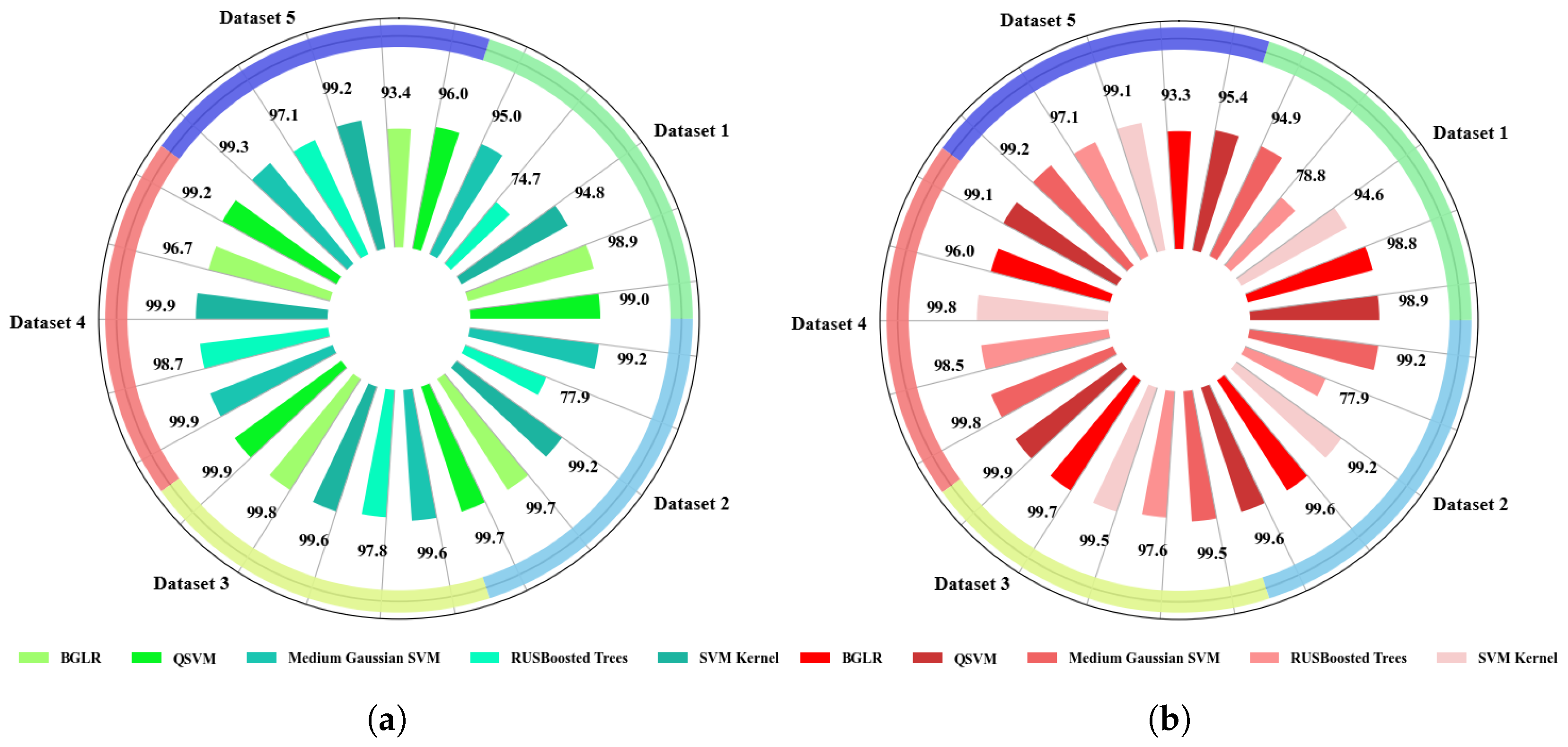
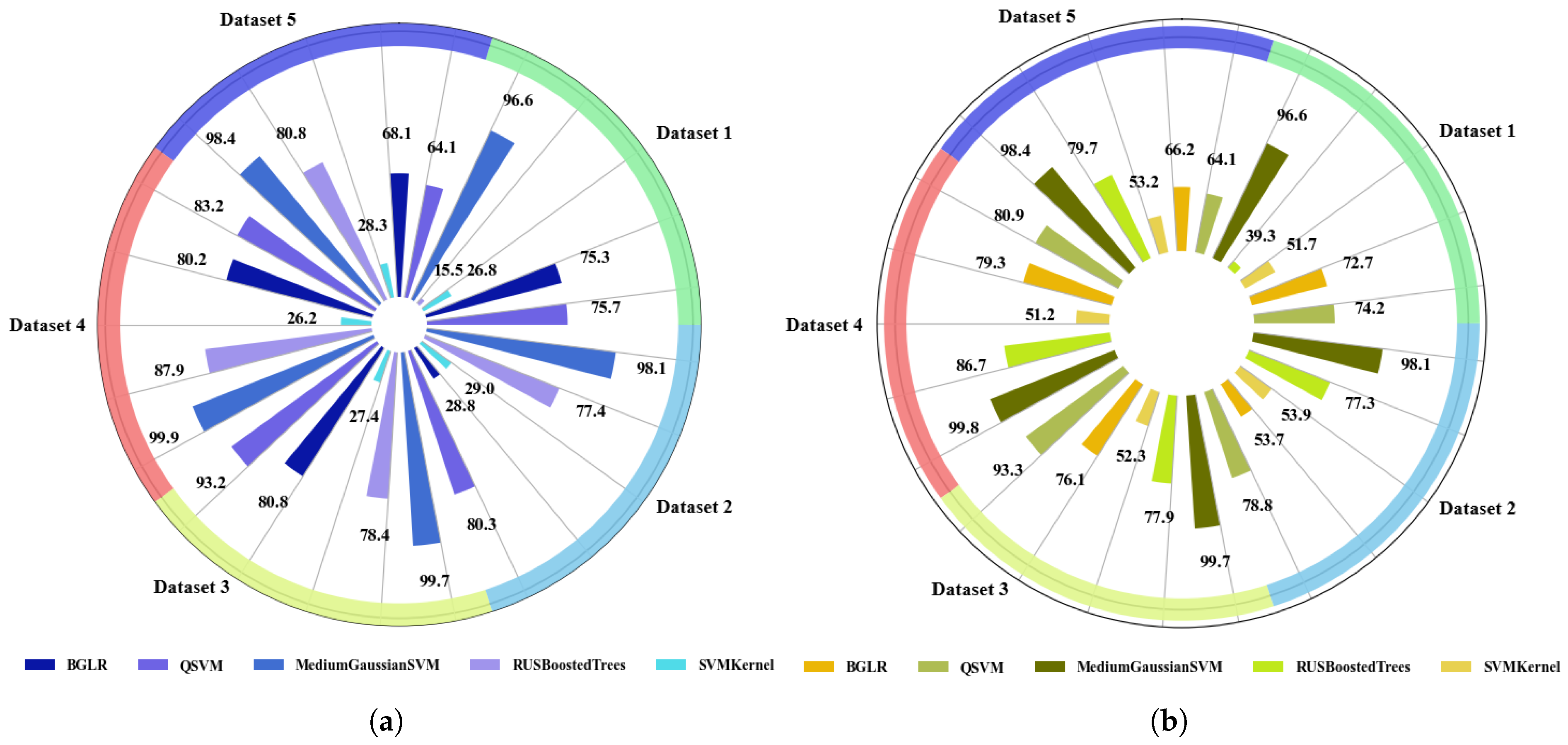
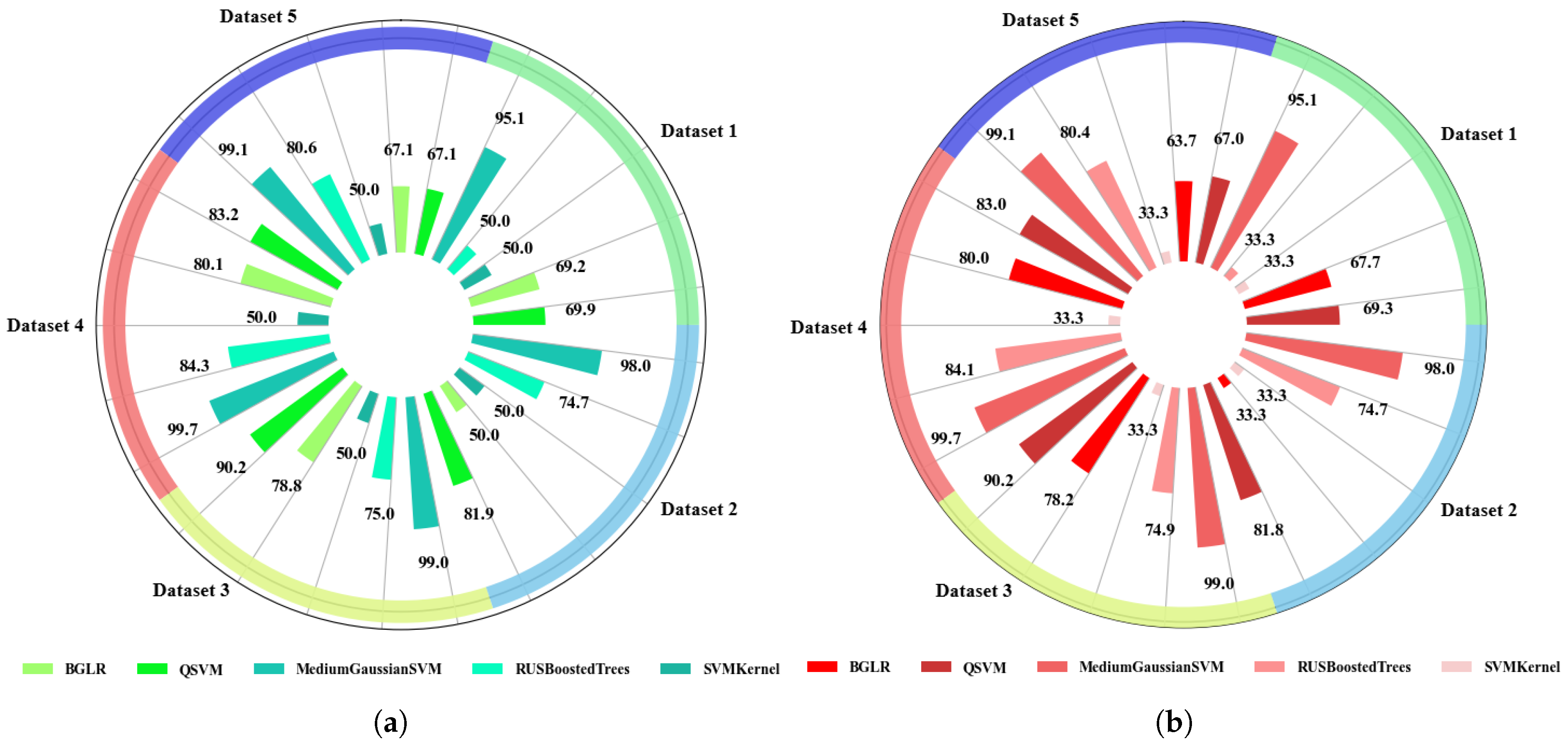
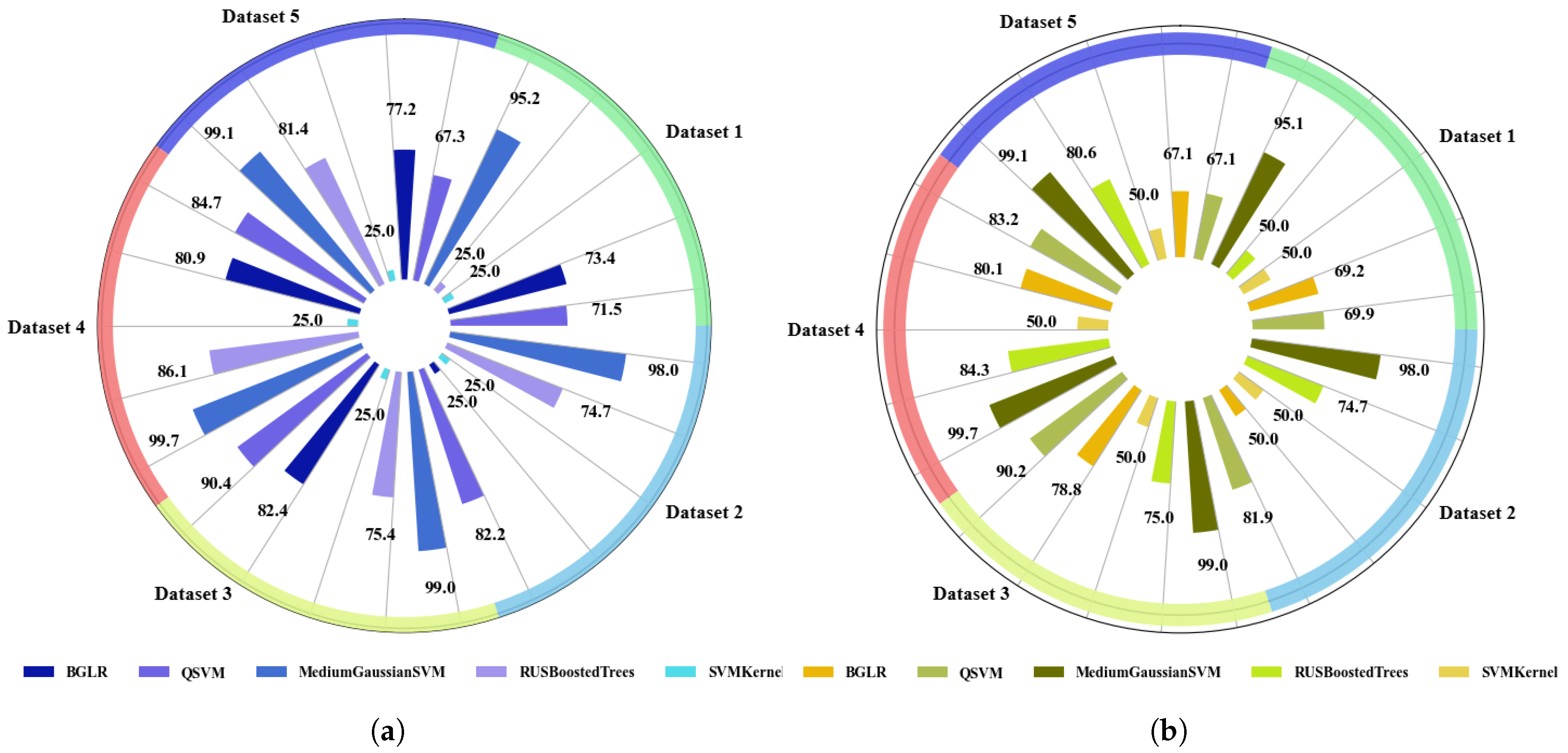
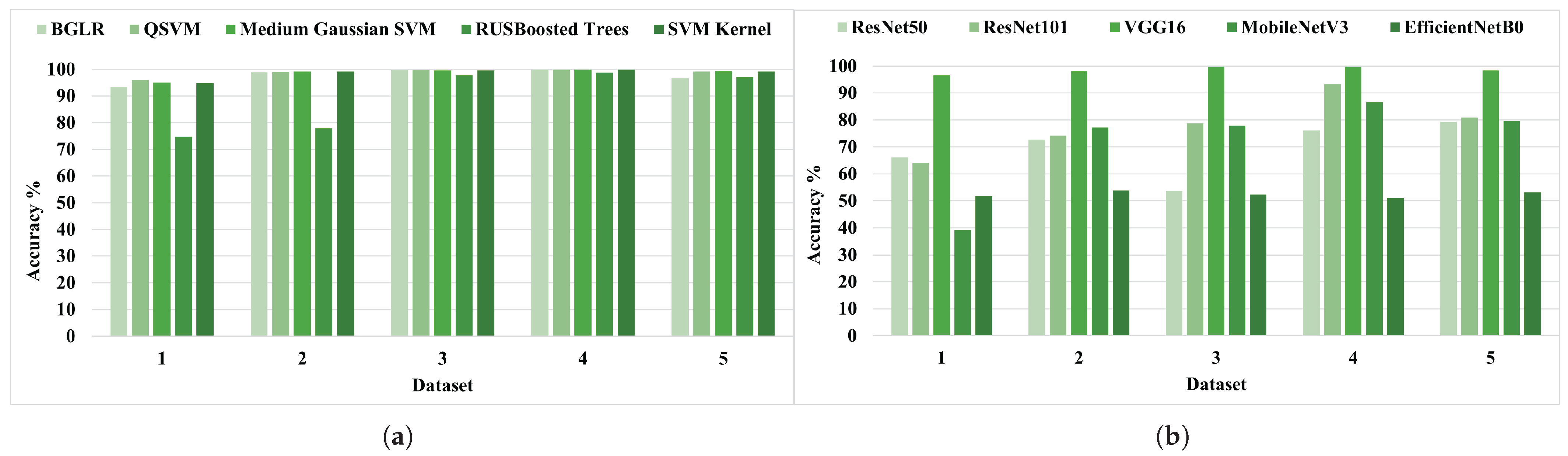
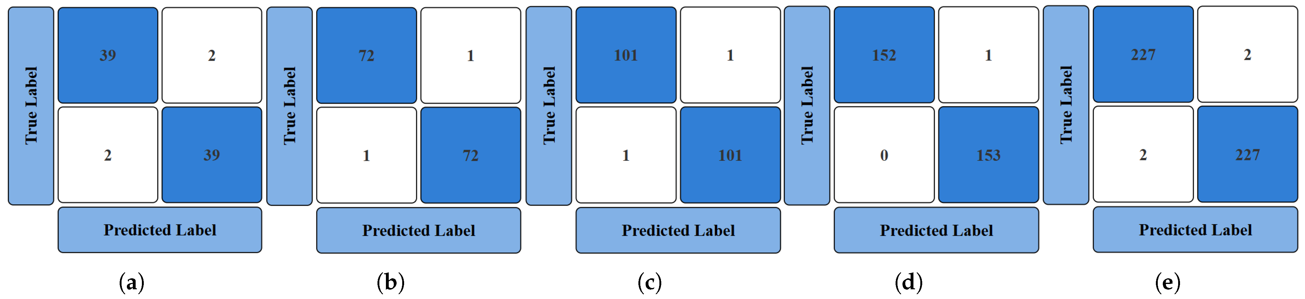
4.1. Comparison of Model Accuracies

Section 4.1.1 and Section 4.1.2 present performance evaluation metrics for the ML and DL models, respectively. Figure 8, Figure 9, Figure 10 and Figure 11 provide training and testing results for ML models, while Figure 12, Figure 13, Figure 14 and Figure 15 present those for DL models.

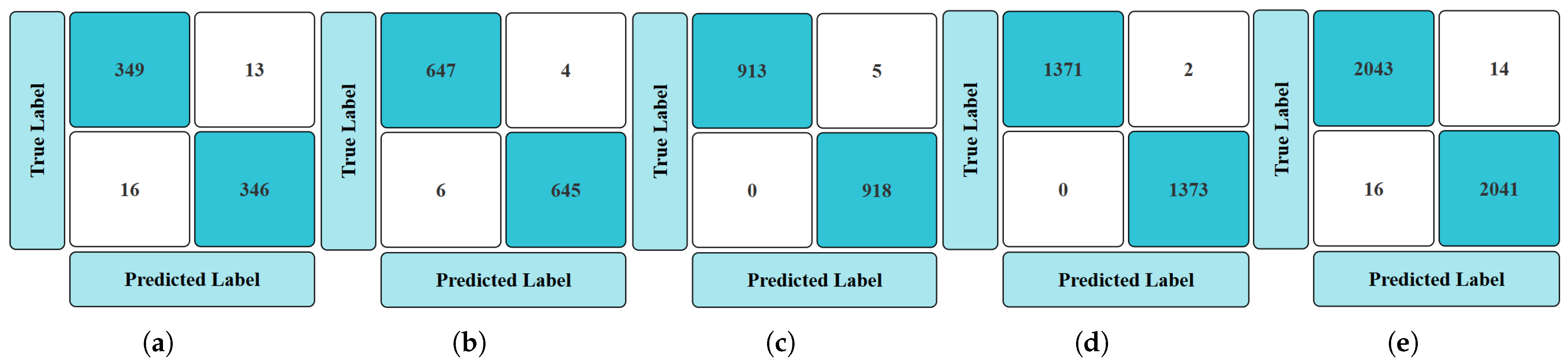
4.1.1. Accuracy Analysis in Traditional ML Models with Extracted Features

It has been emphasized that 31 combinations of features based on CLD, CSD, EHD, HTD and RSD resulted in the best combination of altogether 222 parameters, giving high five-fold cross validation accuracy, which was trained using 34 ML models. Among those models, the top five high-performing models, namely BGLR, QSVM, Medium Gaussian SVM, RUSBosted Trees, and SVM Kernel, were selected and are illustrated by comparative charts. The model performance was analyzed in terms of the training and validation accuracy and testing accuracy of the five ML models, as shown in Figure 8, Figure 9, Figure 10 and Figure 11.

It is observable that 92% of observations fell within the range of 93.4–99.9%, while only 8% were recorded in the range of 74–80%, indicating a strong tendency toward hitting higher accuracy values, as shown in Figure 8a. F1-score, Precision and Recall are illustrated in Figure 8b, Figure 9a, and Figure 9b, respectively. This also follows a similar trajectory, where Precision hits 100% in certain datasets like dataset 3 and dataset 4.

It is observable that all of observations fell above 95%, while Support Vector Machines achieved 100% testing accuracy, according to Figure 10a. In this scenario, the F1-score, Precision, and Recall, illustrated by Figure 10b, Figure 11a and Figure 11b, respectively, exhibit analogous trends, with Precision, Recall, and F1-score attaining 100% in mostly Support Vector Machines.

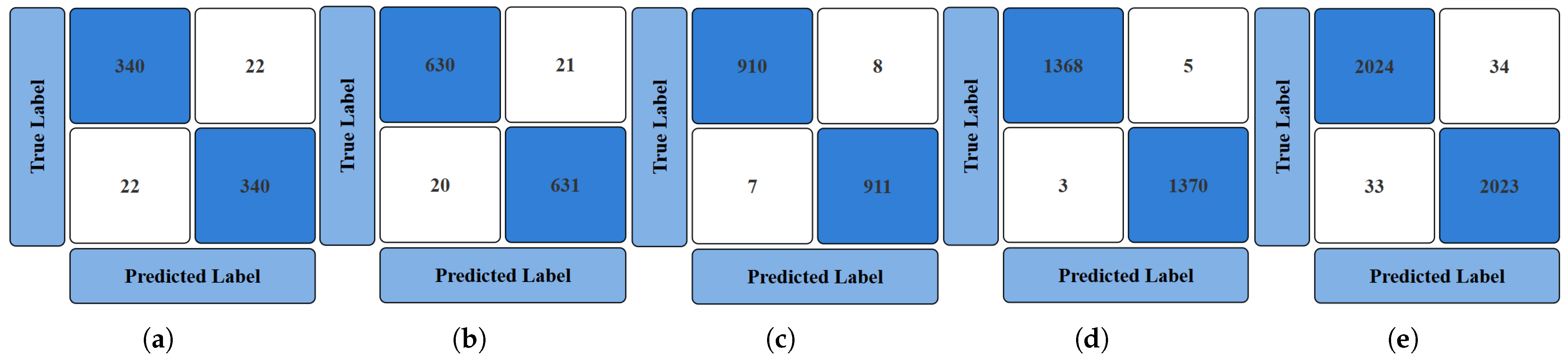
4.1.2. Accuracy Analysis of End-to-End DL

The performance of the model was evaluated based on the training and validation and the testing accuracies of five DL models, as presented in Figure 12, Figure 13, Figure 14 and Figure 15. The model received raw thermal imagery as input.

The analysis revealed that more than 50% of observations fell within the range of 40–80%, while only VGG-16 performed with higher accuarcy according to data in Figure 12a. The minimum value of the F1-score, as shown in Figure 12b, was recorded for MobileNetV3Small; 0.222 which recorded a minimum Precision and Recall of 0.155 and 0.393, as illustrated in Figure 13a and Figure 13b, respectively, for dataset 1. A vast divergence was observed across datasets based on the DL model implemented for resulted performance parameters.

It was observed that 56% of observations result in within the range of 50–80%, in which, altogether, ResNet-50, ResNet-101, VGG-16 and MobileNetV3Small showed above 80% only for dataset 5, as shown in the data recorded in Figure 14a. ResNet-50 maintained a moderate F1-score, Precision, and Recall, as shown in Figure 14b, Figure 15a, and Figure 15b, respectively. Dataset 1 and dataset 2 had a low F1-score and Precision of 0.333 and 0.250, respectively, in each dataset. The minimum value of F1-score was recorded by EfficientNetB0, and it was 0.333. The implemented DL models exhibited significant performance variability across datasets, as measured by key evaluation metrics.

• Accuracy Plots of Training and Testing ML and DL Models

Figure 16 and Figure 17 illustrate a comparative analysis of five ML and five DL models, evaluated under different customized parameter configurations based on accuracies.

According to Figure 16a, ML models show consistency, with high accuracy in training and validation, suggesting that the models are learning effectively. DL models show more fluctuation in accuracy compared to ML models, while some DL models perform quite well, but many others lag behind, as shown in Figure 16b. These noticeable discrepancies were found between training and validation accuracies, particularly in datasets 1 to 3. ResNet-50 and ResNet-101 achieve high training accuracy but suffer significant drops in validation performance, indicating potential overfitting. In contrast, MobileNetV3Small and EfficientNetB0 demonstrate a better balance, suggesting improved generalization for smaller architectures. The observed variation may stem from the differing capacities of the model to generalize across the datasets.

ML models maintain high accuracy in the testing phase as of the illustration in Figure 17a. Having this consistency reinforces that ML models are likely generalizing well and are suitable for deployment in the application of solar panel hotspot classification to be implemented in UAV. The observed similarity between training and testing accuracies across all five ML models indicates an absence of overfitting and reflects a strong generalization capability. This consistent performance across multiple datasets suggests that the ML models are not only effective in learning from the training data but also robust and stable when evaluated on unseen data. The ability to maintain accuracy under varying configurations demonstrates their reliability and makes them suitable for practical deployment in scenarios where data diversity and quality fluctuate. According to Figure 17b, the DL models show variability in testing performance. Although some models generalize well, others show performance drops, suggesting that this variation may be attributed to differences in how well they capture relevant features from input images.

Figure 18 and Figure 19 represent the training phase Confusion Matrices (CMs) of ML models and DL models, respectively, across five datasets. Section 3.1 details the image distribution across the five datasets through Table 1. The number of training images are 724, 1302, 1836, 2746 and 4114.

In Figure 18 and Figure 19 above, the best performing scenarios of both ML and DL are illustrated, showing that ML outperforms DL. For example, regarding the CM of Medium Gaussian SVM on dataset 5, 2043 images were classified as solar hotspot images, while DL classified 2024. When it comes to DL, the overall accuracies are lower in many DL models compared to ML models across varying datasets. Furthermore, this comparison will be elaborated in Section 4.2, where the computational efficiency of the models is analyzed, highlighting that DL models not only perform less consistently but also require significantly more training time than their ML counterparts.

Figure 20 and Figure 21 represent the testing phase CMs of ML models and DL models across five datasets, respectively. The number of testing images are of 82, 146, 204, 306 and 458.

Based on the Confusion Matrices, the ML model shows better performance compared to the DL model. ML achieved perfect accuracy in several cases, for example, 153/153 and 228/229, indicating stronger class-wise prediction. In contrast, the DL model shows slightly more misclassifications such as 2 False Negatives vs. 39 True Positives. For instance, the ML model correctly predicted 227 out of 229 samples in one class, while DL misclassified 2. These results indicate that ML consistently maintains higher Precision and Recall across all tested classes.

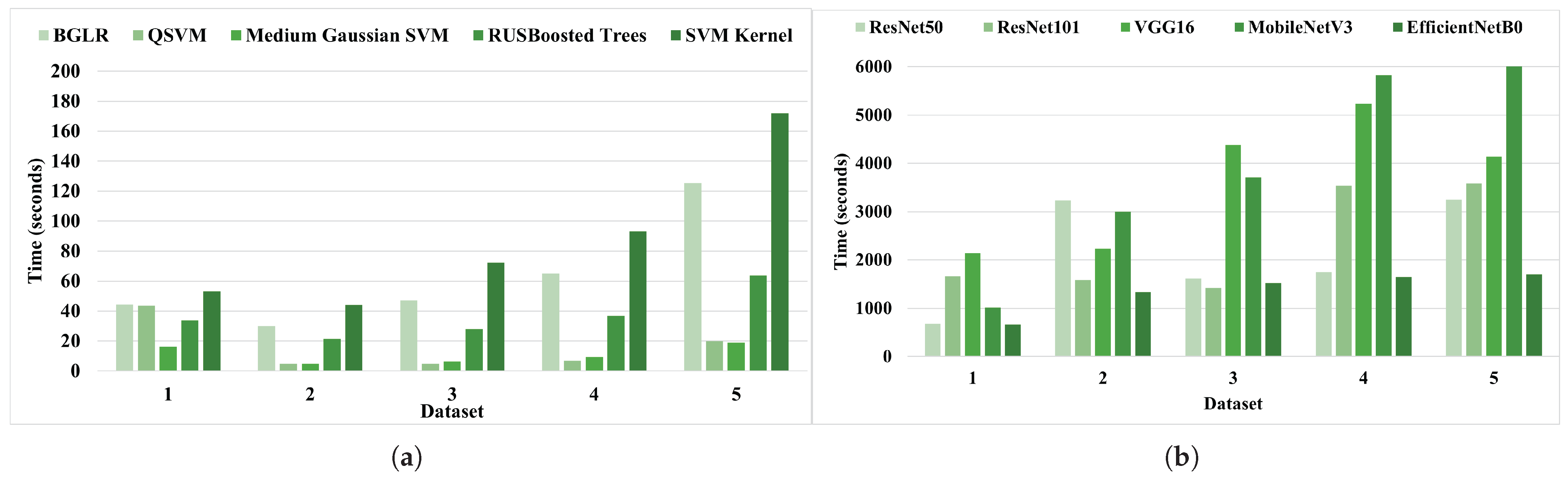
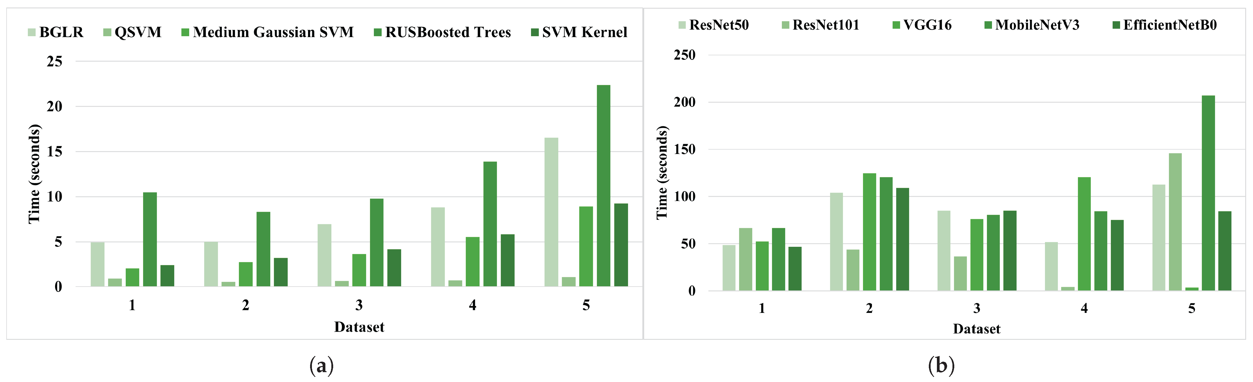
4.2. Resource Utilization Analysis: Computational Efficiency in Terms of Training and Inference Time

To implement a well-informed choice for the appropriate hardware and model, it is essential to consider the training and inference time. DL is rapidly becoming a go-to tool due to its versatility across domains and continuous advancements. Despite its widespread use, it is essential to accurately estimate the time required to train a DL network for a given problem. Therefore, evaluating the time-based computational efficiency between ML and DL models remains a key consideration for targeted applications such as hotspot detection in solar panels.

4.2.1. Resource Utilization Analysis of ML Models

Table 5. Training time (in seconds) of ML models across five datasets.

Training Time (s)
Model	Dataset 1	Dataset 2	Dataset 3	Dataset 4	Dataset 5
Corresponding Number of Images	724	1302	1836	2746	4114
BGLR	44.5	30.1	47.1	65.2	125.4
QSVM	43.6	4.7	4.8	6.8	20.0
Medium Gaussian SVM	16.3	4.8	6.3	9.3	18.8
RUSBoosted Trees	33.8	21.4	28.0	36.8	63.6
SVM Kernel	53.0	44.1	72.4	93.2	171.8

and

Table 6. Testing time (in seconds) of ML models across five datasets.

Testing Time (s)
Model	Dataset 1	Dataset 2	Dataset 3	Dataset 4	Dataset 5
Corresponding Number of Images	82	146	204	306	458
BGLR	4.9	5.1	6.9	8.8	16.5
QSVM	0.9	0.5	0.6	0.7	1.1
Medium Gaussian SVM	2.0	2.7	3.6	5.5	8.9
RUSBoosted Trees	10.5	8.3	9.8	13.9	22.4
SVM Kernel	2.4	3.2	4.2	5.8	9.3

tabulate the training and testing time of top five performing ML models respectively, as given below. The time is in seconds.

SVM Kernel and BGLR exhibit the highest training time, particularly on larger datasets, due to their complexity. For dataset 5, which has a higher number of testing images, the lowest testing time belonged to Medium Gaussian SVM at 18.810 s. For the smallest dataset, despite all five models having a comparatively higher testing time (based on image quality), the Medium Gaussian SVM hits the minimum time of 16.290 s. Therefore, Medium Gaussian SVM is a good candidate when computational efficiency is the key. Overall, it was observed that 96% of the results were below 150.000 s in training time.

The testing time also increases with dataset size, but at a much lower rate compared to training time. RUSBoosted Trees and BGLR tend to have higher testing times, especially on the larger datasets. Medium Gaussian SVM and QSVM show relatively fast inference times, making them suitable for real-time applications. Overall, all models exhibit reasonable testing times, staying below 25.000 s even on the largest dataset.

On the whole, the ML models demonstrate a favorable training–inference balance.

4.2.2. Resource Utilization Analysis of the DL Models

Table 7. Training time (in seconds) for DL models across five datasets.

Training Time (s)
Model	Dataset 1	Dataset 2	Dataset 3	Dataset 4	Dataset 5
Corresponding Number of Images	724	1302	1836	2746	4114
ResNet-50	672.6	3234.6	1614.0	1748.4	3253.2
ResNet-101	1666.8	1585.2	1423.2	3540.6	3580.2
VGG-16	2145.6	2232.0	4374.6	5238.6	4134.0
MobileNetV3Small	1016.4	3003.6	3707.4	5822.4	6003.6
EfficientNet-B0	662.4	1335.6	1518.6	1644.0	1696.2

and

Table 8. Testing time (in seconds) for the DL models across the five datasets.

Testing Time (s)
Model	Dataset 1	Dataset 2	Dataset 3	Dataset 4	Dataset 5
Corresponding Number of Images	82	146	204	306	458
ResNet-50	48.6	103.8	85.2	51.6	112.8
ResNet-101	66.6	43.8	36.6	4.2	145.8
VGG-16	52.2	124.8	76.2	120.6	3.6
MobileNetV3Small	66.6	120.6	80.4	84.6	207.0
EfficientNet-B0	46.8	109.2	85.2	75.0	84.6

tabulate the training and testing time of the DL models, which represents the time in seconds.

Among all the datasets, dataset 2 forces the model to learn fine spatial features that persist across varying drone perspectives, which results in longer training and testing times compared to the other datasets. These high-detail images require deeper feature extraction, thus increasing both the computational load per image and the overall training and testing time.

Among the results of Table 7, EfficientNetB0 shows overall faster training time. ResNet-101 also has a higher training time than ResNet-50; both of these belong to the Residual Network family. MobileNetV3Small attains the highest training time of 6003.6 s.

Among the results shown in Table 8, ResNet-50’s testing time increased from Dataset 2 to 3, but it dropped from 85.2 s to 51.6 s in Dataset 4. ResNet-101 also shows similar scenario at dataset 4, dropping from 36.6 s to 4.2 s. The same is true for dataset 5 in VGG-16 but not in dataset 4. MobileNetV3Small has the highest training time. Overall, DLs’ testing times are higher than ML models’ testing times.

• Time Plots of Training and Testing ML and DL Models

Figure 22 and Figure 23 present a comparative analysis of five ML and five DL models, assessed under various custom parameter settings with respect to training and testing time.

According to Figure 22a, ML models show very low training time across all datasets, mostly under 200 s. This highlights the computational efficiency of ML models. Their lightweight nature makes them suitable for applications where training time is a constraint, such as real-time or edge computing scenarios.

As illustrated by Figure 22b, DL models require significantly more time, reaching up to approximately 6000 s in certain scenarios. DL models are computationally intensive due to their complex architectures and iterative optimization processes. The inclusion of training overhead like model compilation and loading further increases the total time. This is a key consideration in deployment scenarios where resources or time are limited.

ML models demonstrate low latency during testing, with most below 25 s, according to the chart in Figure 23a. This fast inference time reinforces the feasibility of ML models for real-time decision-making tasks or embedded systems.

DL models show moderate testing times. However, it is significantly higher than ML models, some of which are beyond 200 s, as shown in Figure 23b. While the inference time remains within tolerable margins for many applications, the extra delay could be problematic in systems where the prompt response is essential.

4.3. Computational Efficiency Analysis of ML and DL Models

Although numerous studies on thermal-image feature extraction focus primarily on classification accuracy, they often neglect computational efficiency, which is an equally critical aspect for real-world deployment. This omission is particularly significant for Unmanned Aerial Vehicle (UAV)-based applications, where onboard systems operate under strict constraints on memory, processing power, and energy availability. In such environments, models must be not only accurate but also lightweight and fast enough to support real-time inference. To bridge this gap, the present study provides a detailed computational-efficiency analysis of five top-performing ML and five DL models across multiple datasets, with a specific focus on their suitability for UAV deployment.

In Section 4.3, Table 5, Table 6, Table 7 and Table 8 summarize the training and testing times for each model type, with times measured in seconds across different datasets. These models were selected for their strong performance in thermal image classification tasks.

• ML Models

Table 5 provides the training time for each of the five ML models across the datasets, while Table 6 details the testing times. The training time increases with the dataset size, as expected. Models like SVM Kernel and BGLR exhibit significantly higher training times, due to their inherent complexity. However, Medium Gaussian SVM consistently shows lower training times compared to others, with times under 20 s considering all the datasets. This makes it a strong candidate when computational efficiency is critical, particularly for UAV-based systems.

In terms of testing times, the analysis in Table 6 reveals that RUSBoosted Trees and BGLR exhibit the highest testing times, especially with datasets with a high number of images. On the other hand, Medium Gaussian SVM and QSVM provides faster inference times, well below 10 s for the largest datasets. These characteristics of low testing time and moderate training time make them ideal candidates for real-time applications and resource-constrained environments, such as those encountered in UAV-based monitoring.

• DL Models

In contrast, DL models, such as ResNet-50, VGG-16, and MobileNetV3Small, demonstrate significantly higher computational demands, as detailed in Table 7 and Table 8 for training and testing times, respectively. Models like VGG-16 and MobileNetV3Small require several thousand seconds for training for all datasets, making them less practical for real-time deployment on UAVs, where resource constraints are critical. For instance, MobileNetV3Small requires 1016.4 s for training on dataset 1, while it reaches 6003.6 s on dataset 5, clearly indicating its high computational overhead.

In terms of inference times, ResNet-50 and ResNet-101 exhibit increased testing times compared to the ML models, often exceeding 100 s. While EfficientNetB0 and MobileNetV3Small show slightly better inference times, the DL models still tend to be slower, with testing times as high as 207 s for MobileNetV3Small on dataset 5.

• Implications for UAV Deployment

The detailed analysis clearly illustrates the trade-off between model accuracy and computational efficiency, especially in the context of UAV deployment. ML models, particularly Medium Gaussian SVM, offer a significant advantage in resource-constrained UAV settings, where computational power and processing time are limited. These models not only achieve high accuracy but also ensure low training and inference times, making them ideal for real-time analysis in UAV applications.

On the other hand, while DL models offer state-of-the-art accuracy, their high training and inference times make them less suitable for scenarios where resource availability and real-time decision-making are critical. UAVs equipped with limited processing power may face challenges in deploying these models effectively, particularly when processing large datasets in a timely manner.

In conclusion, the analysis of the computational efficiency of both ML and DL models underscores the need to prioritize efficiency alongside accuracy when selecting models for UAV-based thermal image monitoring, especially in resource-constrained environments. Medium Gaussian SVM emerges as a favorable choice due to its low computational demand with fast inference times, making it highly suitable for deployment in real-time applications. By carefully considering both accuracy and computational efficiency, optimal performance should be achieved for UAV-based hotspot detection systems.

4.4. Understanding the Constraints of DL Performance

DL models, while powerful, exhibit noticeable variability in both training and testing performance across datasets. Unlike traditional ML models, which consistently generalize well with minimal performance drop, DL models such as ResNet-50 and ResNet-101 often show signs of overfitting, achieving high training accuracy but experiencing a decline in test set performance, especially in datasets 1 to 3. This discrepancy suggests that deeper models have difficulty generalizing when exposed to diverse data. In contrast, lighter architectures like MobileNetV3Small and EfficientNetB0 perform more consistently, indicating that smaller models offer better generalization under changing data characteristics. This variation arises not only from model complexity but also from differences in feature extraction capabilities across datasets.

In addition to accuracy-related challenges, DL models also encounter computational limitations. As dataset size increases, training time grows significantly. Although EfficientNetB0 demonstrates improved efficiency, it still falls short compared to lightweight ML models such as Medium Gaussian SVM in both training and inference times. Real-time deployment scenarios, such as UAV-based solar panel inspection, benefit from models that deliver faster inference and stable accuracy. DL models, though capable of capturing complex patterns, may not always provide the best trade-off between performance and computational efficiency. These limitations highlight the importance of selecting architectures suited to application-specific requirements, including data variability, inference speed, and resource availability.

As shown in

Table 9. Comparison of VGG16 (DL) vs. Medium Gaussian SVM (ML) across five datasets in terms of classification accuracy (%) and training time in seconds.

Model	Dataset 1		Dataset 2		Dataset 3		Dataset 4		Dataset 5
	Acc. (%)	Time (s)	Acc. (%)	Time (s)	Acc. (%)	Time (s)	Acc. (%)	Time (s)	Acc. (%)	Time (s)
VGG16 (DL)	96.55	1016.4	98.08	3003.6	99.73	3707.4	99.82	5822.4	98.42	6003.6
Medium Gaussian SVM (ML)	95.00	16.29	99.20	4.76	99.60	6.32	99.90	9.31	99.30	18.81

Note: Acc. refers to accuracy.

, Medium Gaussian SVM achieved similar or superior accuracy to VGG16 across all datasets while requiring only a fraction of the training time. This underscores the efficiency and practicality of ML models for real-time or embedded applications.

In summary, the results provide strong evidence that ML models exhibit superior overall performance compared to DL models. ML models are consistently faster to train and test, making them more efficient for quick-deployment scenarios. For resource-constrained environments, ML models are more favorable when computational resources and time are a concern. Based on the observed results, it can be confidently concluded that ML models outperform DL models overall performance-wise.

5. Discussion

Based on the results, it is observed that Medium Gaussian SVM and Quadratic SVM perform well out of the top five models selected. With the training and testing results for performance and time evaluation, Medium Gaussian SVM achieves 99.3% accuracy, and it achieved higher accuracy across five datasets in training scenarios. Considerably, its training and testing times are also low but resulted in the minimum time for quadratic SVM. This is outweighed by other factors such as the ability to handle nonlinear patterns, better generalization for datasets with irregular distributions, flexible boundaries that fit the real-world data, a Gaussian kernel that adapts to complex decision boundaries, and the capturing of minor differences between hotspot and non-hotspot regions. The Gaussian kernel has the capability to control boundary smoothness by kernel scale parameter. Above all, Medium Gaussian SVM is widely used for proven performance in vision tasks. This shows good performance in high-dimensional feature spaces.

This section elaborates on the interpretation of the most impactful features influencing solar hotspot classification predictions using What-if Analysis, highlighting key trends and insights. Furthermore, it presents an in-depth discussion of the advantages of the ML approach in addressing limitations commonly encountered with DL-based methods. A comprehensive comparison between the proposed method and prior techniques is conducted, including a boxplot analysis that visualizes the performance differences between ML and DL models. Additionally, statistical validation is employed. Furthermore, this section analyzes the trade-offs between classification accuracy and computational resource utilization. These discussions collectively serve to clearly position this research within the context of the existing literature.

What-if Analysis complements the interpretability objectives of this research by providing a simulation-based validation of feature sensitivity in ML models. Unlike DL models, which often function as black-box systems, ML models allow for fine-grained control and analysis of individual feature impact. The results from What-if Analysis provide empirical evidence of how changes in critical features such as average blue chroma and luminance influence the model’s prediction, thus offering an additional layer of transparency. This directly supports the broader scope of the paper, which advocates for explainable, resource-efficient ML models over DL models for solar hotspot classification.

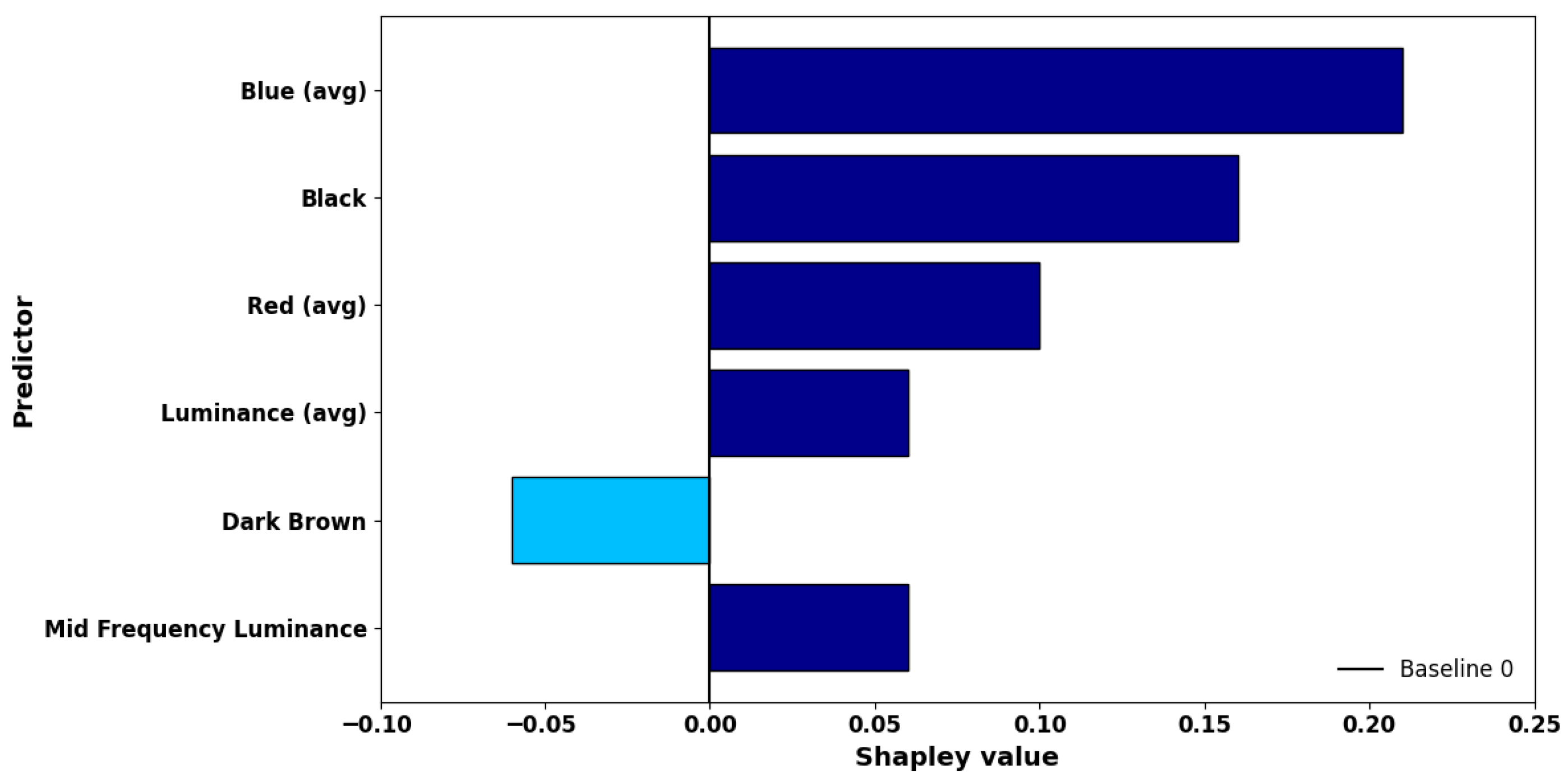
5.1. Local Interpretation of Input Feature Contributions Using SHAP for ML Model Predictions

The analysis is based on feature space extracted for model training and testing. The query point represents data instances, while the Shapley plot visualizes how much each feature contributed to the prediction of a model for a given query point, which both are used in XAI. The bar plots below illustrate the absolute contribution of each feature. The Shapley value of a feature is the average marginal contribution it makes to the prediction across all possible feature combinations.

SHAP analysis was conducted to interpret the predictions of the model and identify the most impactful features for classification. Blue (avg) in Figure 24 refers to the DC coefficient for the Cb (blue-difference chroma) channel, representing the average blue component feature in the Color Layout Descriptor, which demonstrates the dominant colors and their spatial distribution. The blue-difference chroma means that a high Cb value refers to more blue in the image and a low Cb value refers to less blue and more yellow or red instead. It captures temperature variations more effectively in the YCbCr color space. This is the most effective in detecting cooler vs. hotter regions of an image.

5.2. What-If-Analysis

What-if Analysis results for the image in Figure 25 illustrate the individual impact of each feature on the model output. The initial query point was set to default values, and the corresponding Shapley values are presented in Figure 26. Figure 27 and Figure 28 compare two scenarios: Figure 27a,b and Figure 28a,b correspond to Scenario 1, where the average blue value (blue-avg) was varied, and Figure 27c,d and Figure 28c,d correspond to Scenario 2, where the average luminance (luminance-avg) was adjusted. In both scenarios, the modified feature was incremented from 0 to 1 in steps of 0.1. Scenario 1 resulted in significant shifts across multiple features, including black, red (avg), luminance (avg), dark brown, and mid-frequency luminance. Scenario 2, by contrast, produced only minor changes in these features. Detailed visualizations of the minimum and maximum custom points, corresponding to 0 and 1 respectively, are shown in Figure 27 and Figure 28.

The diagrams presented in Figure 26, Figure 27 and Figure 28 illustrate the query point alongside local Shapley explanation plots. In each figure, blue dots represent the data instances that refer to query points. The selected query point is marked in an encircled black dot, while custom point in each image is indicated by a green square.

Figure 26 depicts the baseline scenario, where all custom feature values remain at their original settings. Specifically, Figure 26a,b show the query point and the corresponding local Shapley explanation for the default values of average luminance (0.127) and blue chrominance (0.8314), respectively. In Figure 26a, the original and custom points fully overlap, indicating no feature variation. In Figure 26b, the alignment of light-brown and dark-brown bars in the Shapley plot demonstrates that feature contributions remain consistent at the default values.

According to Figure 27a, when the blue (avg) value was set to 0, its Shapley value started from negative, as shown in Figure 27b. There are notable variations in other features, such as black, red, and mid-frequency luminance, due to its impact. On the otehr hand, when the luminance (avg) was set to the same value of 0, as shown in Figure 27c, its Shapley value stayed on the positive axis, representing a higher value. In this adjustment, the influence of other characteristics remained predominantly unchanged, with minimal variation as in Figure 27d.

According to Figure 28a, setting the average blue value to 1.0 caused its Shapley value to exceed its original point and continue rising, indicating an upward trend, as shown in Figure 28b. This adjustment resulted in slight deviations in related features such as black, red, and mid-frequency luminance. On the other hand, setting the average luminance to 1.0, as shown in Figure 28c, led to a gradual and consistent increase in its Shapley value. In this case, other features experienced negligible changes, showing consistent behavior throughout, as evidenced in Figure 28d.

Overall, when the average blue value was increased from 0 to 1 in steps of 0.1, the corresponding Shapley value shifted from negative to strongly positive, indicating an increasing contribution to the prediction according to Figure 27 and Figure 28. This change was accompanied by notable variations in other features, such as black, red, and mid-frequency luminance. In contrast, when the average luminance varied over the same range, its Shapley value gradually decreased from slightly positive to negative. During this adjustment, the influence of other features remained largely consistent, showing minimal variation.

The average blue value is a key and influential feature in identifying hotspots. As the blue value changes, the importance of other features also shifts, suggesting that the model adjusts their influence based more on blue. For instance, when blue (avg) is low, features like black or red (avg) may become more important to support the prediction.

The presence of hotspots creates strong local contrast in the blue channel, causing the overall average blue value to drop. As a result, the average blue becomes a contrast-sensitive and useful feature for distinguishing hotspots. Equations (7) and (8) are formulated per unit area of a solar panel with a hotspot.

$$X_{\mathrm{rel}}=X_{\mathrm{panel}}-X_{\mathrm{abs}}$$

(7)

$${\varphi }_{\mathrm{blue}}\propto X_{\mathrm{rel}}$$

(8)

where $X_{\mathrm{rel}}$ represents relative blue difference, $X_{\mathrm{panel}}$ represents the absolute blue channel mean value of the hotspot region, $X_{\mathrm{abs}}$ represents the average blue channel mean across the background solar panel, and ${\varphi }_{\mathrm{blue}}$ represents SHAP value associated with the blue channel.

Therefore, there is a positive value of $X_{\mathrm{rel}}$ when the blue mean region is lower than the panel, and the average implies a positive SHAP contribution, which supports classification as a hotspot. Conversely, when the region is relatively bluer than the panel background, it contributes negatively to the hotspot class prediction. This formulation provides a locally linear explanation for the behavior of the model in terms of relative blue suppression due to elevated temperature in hotspot regions.

SHAP evaluates features in a relative context, comparing feature values of each region against the background distribution. The variable blue (avg) in the model does not directly mean the visible degree of blueness of a region. Instead, it reflects the numerical intensity of the blue channel, which interacts with contrast against neighboring colors like yellow, red, and brightness.

The blue (avg) feature acts as a contrast indicator, which is not just about how blue a region is but how much less blue it is compared to surrounding areas. In solar images, yellow hotspot regions reduce the blue channel, making the blue (avg) lower there than in normal areas. This drop in blue helps the model detect hotspots, and SHAP values reflect this by highlighting blue (avg) as an important feature in the decision process.

These What-if scenarios not only demonstrate how sensitive the model’s decisions are to changes in individual features but also underscore the strength of ML models in enabling localized interpretability. This level of explanation is inherently difficult to extract from DL models, which typically rely on deep layers of abstraction. By showing how model outputs respond predictably to controlled changes in feature values, What-if Analysis reinforces the claim that ML models are more suitable for deployment in scenarios that demand both predictive performance and interpretability, such as UAV-based real-time solar inspections.

Finally, in solar panel thermal inspection, both the actual temperature and the difference from nearby areas are important. However, the relative drop in blueness often gives the most useful indication for early-stage issues, even at the stage in which the hotspot is not extremely hot. For solar panel thermal inspections, both absolute and relative temperature changes matter, but the relative drop in “blueness” is often the key diagnostic clue for faults.

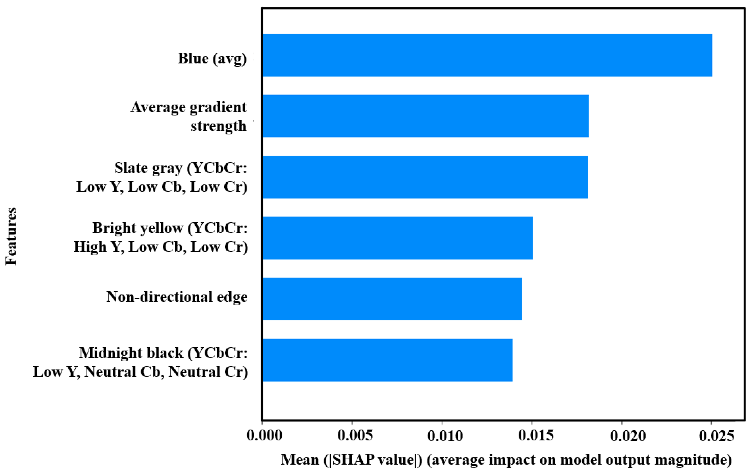
5.3. Global Interpretation of Feature Importance Using the SHAP Summary Plot for Solar Hotspot Detection in Thermal Imagery Classification

Figure 29 shows a SHAP summary plot that illustrates the six most impactful features influencing the model output for solar hotspot classification. The x-axis indicates the mean absolute SHAP value, which represents the average contribution of each feature represented on the y-axis to the model decision. This plot provides a clear overview of the most influential input features based on their impact magnitude.

The SHAP analysis highlights that the model for solar hotspot classification relies heavily on color and edge-based features, with blue chrominance (avg Cb) emerging as the most influential factor. Importantly, this feature acts not just as an absolute measure of blue intensity, but as a contrast-sensitive indicator, capturing relative drops in blueness due to elevated temperatures in hotspot regions. In thermal imagery, yellow or red hotspots suppress the blue channel, lowering the average blue value in those areas. This contrast, if a region is less blue compared to the surrounding panel background, this enables the model to recognize early-stage faults, even before extreme heating occurs. Thus, blue (avg) becomes a contextual reference point: when a region is relatively less bluer than the panel, it contributes positively, indicating a potential hotspot. SHAP values capture this local behavior, showing that the model dynamically adjusts the weight of other features based on the level of blue, reinforcing blue (avg) as a locally linear and contrast-driven discriminator.

Because blue chrominance is largely invariant to illumination and decouples color from brightness, it offers a robust and stable cue for distinguishing healthy regions. This reliability across different conditions explains why blue (avg) holds the highest SHAP value and serves as the primary suppressive signal of the model for ruling out hotspots.

In contrast, bright yellow regions characterized by high Y, low Cb, and low Cr values are often associated with elevated temperatures but remain context-sensitive. Such yellow hues may arise not only from true thermal anomalies but also from normal solar heating or environmental reflections, making them a less definitive indicator of hotspots. Consequently, the model assigns these features moderate importance, interpreting them more reliably when assessed in conjunction with other cues such as edge patterns or local suppression of blue chrominance. Although the statistical validation of MPEG-7 descriptors in Section 5.7.3 confirms that yellow regions are significantly more prominent in hotspot areas, the SHAP-based interpretation reflects a cautious weighting of these features. This is likely due to their potential variability under different imaging conditions. Therefore, yellow-based cues contribute most effectively to hotspot detection when contextualized by complementary indicators like blue contrast and edge activity.

Meanwhile, slate gray (low Y, low Cb, low Cr) contributes notably by providing localized thermal contrast. While less prominent than blue, it often marks regions of early degradation or transition zones, especially where it borders warmer colors like yellow or red. This border contrast enhances the sensitivity of the model to subtle faults or developing hotspots.

Ultimately, while multiple features work in concert, it is the relative decrease in blueness—not just its presence, that emerges as the most diagnostically valuable cue for early-stage hotspot detection. This makes blue (avg) not only the most impactful feature of SHAP ranking but also the most physically and contextually grounded for reliable solar thermal analysis.

5.4. Comparative Analysis of ML and DL Models for Thermal Image Classification

Among the results, the comparative analysis between traditional ML models and DL models clearly demonstrates the superior performance of ML techniques in this study. Across all five datasets, the ML models consistently outperformed the DL models in terms of Accuracy, F1-score, Precision, and Recall. For instance, in the testing phase, Figure 10 and Figure 11 vs. Figure 14 and Figure 15, Support Vector Machine (SVM) models, including QSVM and SVM Kernel, achieved very high accuracy, with F1-scores, Precision, and Recall also reaching their maximum values, indicating near-perfect classification in several cases. Notably, the Medium Gaussian SVM attained high accuracy of 99.3% on the largest dataset (Dataset 5), with an inference time of just 18.8 s, showcasing its efficiency and scalability. In contrast, DL models like ResNet-50 and MobileNetV3Small showed considerably lower performance, often yielding much lower accuracies, and F1-scores below 0.400, which falls within the poor performance range. Even among DL models, only the VGG-16 approached competitive accuracy, but its performance was still less consistent across all datasets compared to ML models. This pronounced contrast in results underscores the robustness and reliability of ML models with handcrafted feature extraction when applied to thermal image classification tasks, especially in scenarios with distinct feature distributions.

5.5. In-Depth Discussion of the Advantages of ML over the Limitations of the DL Approach

The ACE Media Tool performs well in domain-specific tasks. The features extracted are interpretable, since handcrafted features have clear meanings such as color and texture patterns, and hence, it is easier to understand and interpret. In contrast, pre-trained DL models are designed to be general-purpose. The features extracted are less interpretable when DL models act as “black boxes”. Techniques like feature visualization or saliency maps can help but are not as intuitive as handcrafted features. Therefore, it is essential to focus on the deployment of the ACE Media Tool in feature extraction for specific industrial applications like solar PV hotspot classification. It was observed that several feature descriptors have been investigated to figure out the best matching option for reaching a high accuracy of the classification model.

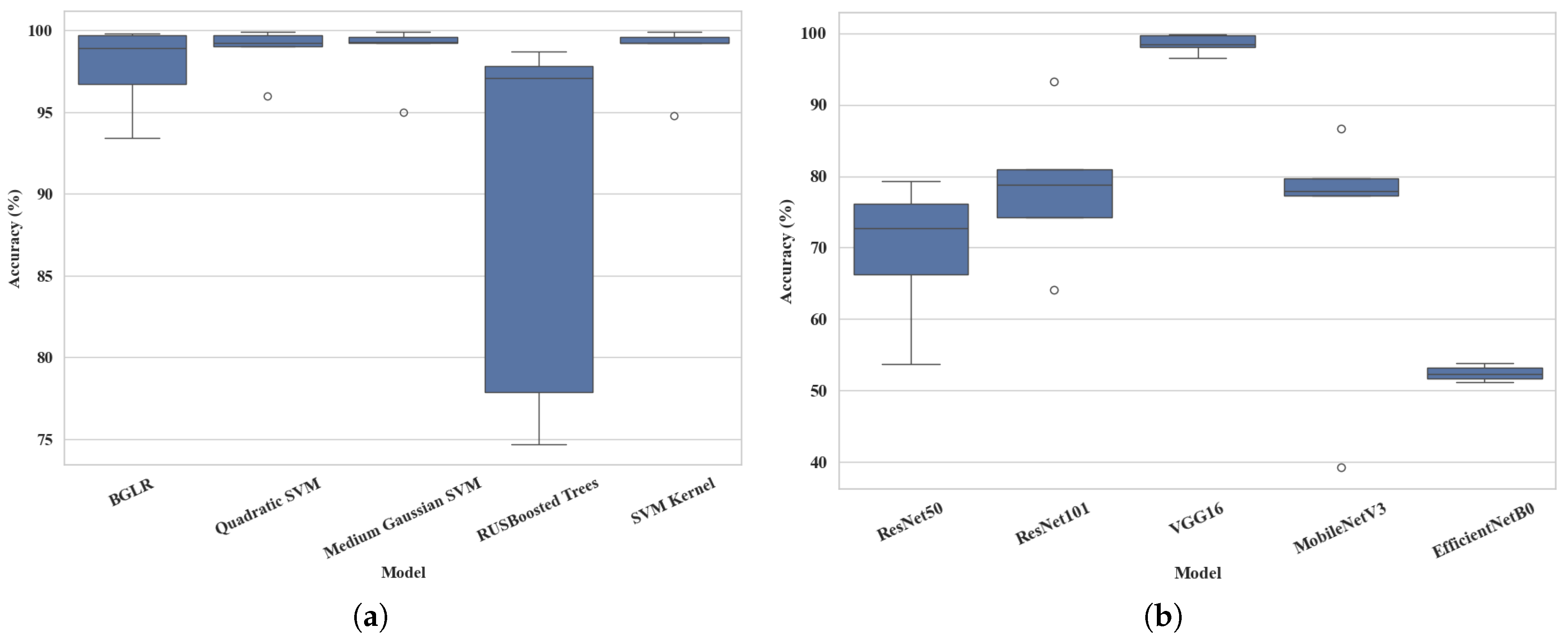
5.6. Comparative Boxplot Analysis on Performance of ML and DL Models

The two boxplots provide a comparative analysis of the accuracy of various ML and DL models across multiple datasets, as shown in Figure 30.

In the plot of ML models, the overall accuracy is higher and more consistent compared to the DL group. Medium Gaussian SVM stands out as the best-performing model, demonstrating consistently high accuracy with minimal variation across datasets. Quadratic SVM also shows strong and stable performance with very little fluctuation. Binary GLM Logistic Regression maintains relatively high accuracy with a slightly broader range. RUSBoosted Trees, while sometimes effective, shows the widest spread and a clear drop in minimum accuracy, indicating less consistent behavior.

In comparison, DL models show more variability and generally lower accuracy. VGG-16 delivers the strongest performance among DL models, with relatively high and stable accuracy. MobileNetV3Small and ResNet-101 perform moderately well, though MobileNetV3Small exhibits an outlier that suggests instability in certain cases. ResNet-50 shows broader variation and a lower median accuracy. EfficientNetB0 ranks lowest among all DL models, with a narrow band of lower accuracy values. Compared to the ML models, the DL models exhibit more frequent and extreme outliers, as illustrated by circles, highlighting their inconsistent performance across datasets.

In conclusion, ML models, particularly Medium Gaussian SVM, outperform DL models in both accuracy and consistency. While VGG-16 is the most reliable among DL models, it does not match the top-tier performance seen in ML models, reaffirming the strength of traditional ML techniques in this evaluation.

5.7. Analysis of Trade-Offs Between Accuracy and Resource Utilization

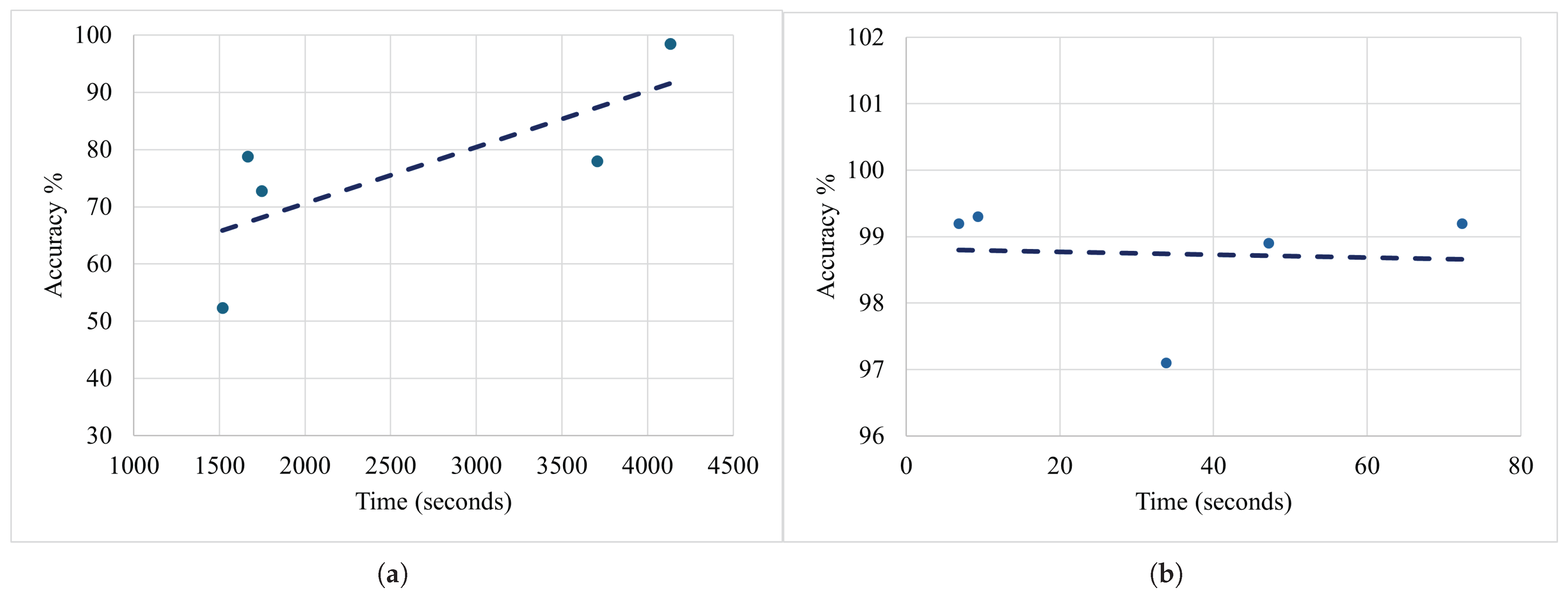
5.7.1. Evaluating Training Efficiency: Accuracy vs. Time in DL and ML Models

The charts in Figure 31 illustrate how accuracy changes over time during the training phase of both the ML and the DL models. The dots represent the median accuracy across five datasets plotted against training time, while the dashed line indicates the overall trend.

A clear trend is observed in Figure 31a, where accuracy generally increases with longer training time, with the insight that longer training tends to result in higher accuracy. However, some fluctuation indicates that not all models equally benefited from longer training durations. Although longer training times often lead to higher accuracy, this relationship is not always consistent across all models or datasets. The variability could also be attributed to the sensitivity of certain models to different datasets.

A noticeable trend is evident, namely that accuracy is consistently high at 97–99% across very short training times, such as below 80 s, given the perception that ML models train significantly faster than DL models while achieving high accuracy, as shown by the illustration in Figure 31b. There is minimal variation in accuracy with the increased training time as the models reach an optimal performance rapidly. It can be concluded that ML models offer efficient training with consistently high performance, making them ideal for fast deployment scenarios.

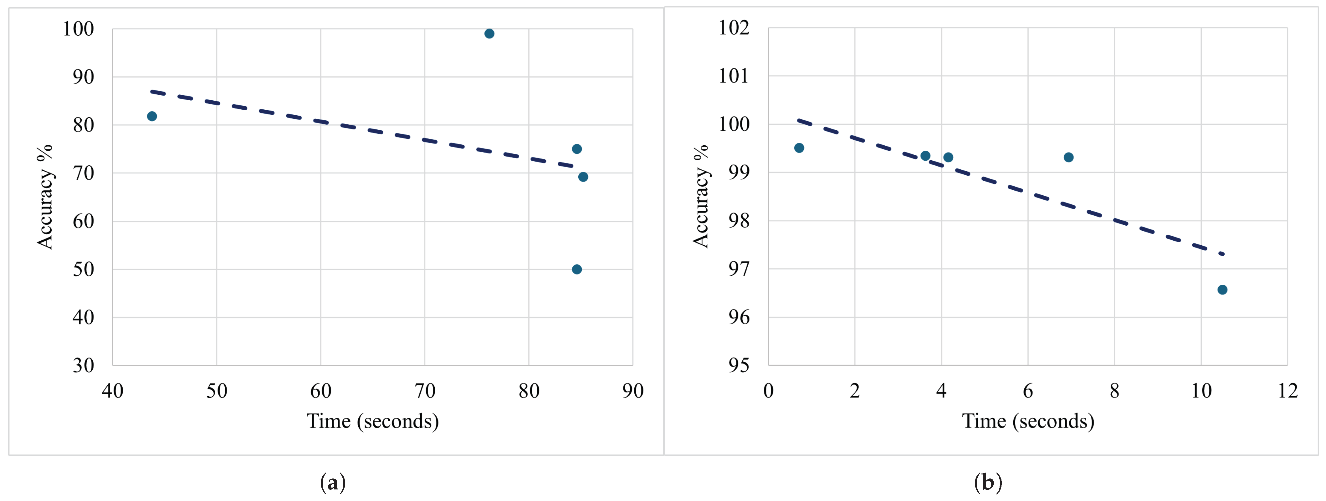
5.7.2. Evaluating Testing Efficiency: Accuracy vs. Time in DL and ML Models

The charts in Figure 32a,b illustrate how accuracy changes over time during the testing phase of both ML and DL models.

Figure 32a depicts that the accuracy fluctuates and slightly decreases with increased testing time. Some deep models are more computationally expensive without offering better accuracy. It is evident that there is negative correlation between testing time and accuracy. Overall, more complex DL models can be inefficient in terms of inference time.

Accuracy is very high in the range of 97–99% across all testing times below 12 s, with the proven insight that training ML models maintains high performance with very fast testing times, as shown in Figure 32b. Time differences are minimal, suggesting all tested models are lightweight. Therefore, it is justifiable to conclude that ML models are extremely efficient at inference, with very little cost to performance, showing great generalization with minimal delay.

5.7.3. Statistical Validation of MPEG-7 Feature Behavior in Hotspot vs. Non-Hotspot Regions

To validate the discriminative strength of MPEG-7 descriptors in thermal hotspot detection, a comprehensive statistical analysis was conducted across five datasets. This evaluation examines the significance, effect size, and reliability of key features using standard statistical metrics, including p-values, t-statistics, Cohen’s d, correlation coefficients, and confidence intervals. These metrics collectively assess how effectively each descriptor differentiates between panels with and without thermal anomalies.

In thermal images of solar panels, specific MPEG-7 features effectively distinguish between panels with and without hotspots. The HTD captures textural differences; panels without hotspots typically exhibit a low mean and a high inverse difference moment, reflecting uniform surface temperature and smooth texture. In contrast, panels with hotspots show a higher mean and lower homogeneity due to abrupt intensity changes caused by thermal anomalies. The EHD, particularly the vertical edge component, is also informative; in non-hotspot panels, edge activity is minimal, whereas hotspot-affected panels show increased vertical edge strength where hotspots disturb the texture. A vertical edge is a region where there is a strong horizontal change in intensity; that is, pixel values change sharply from left to right. If a model sees higher vertical edge counts and texture irregularities, it can infer that a thermal anomaly, that is, a hotspot, is present. Additionally, the CSD reveals chromatic patterns linked to temperature; regions characterized by Warm Yellow (YCbCr: High Y, Low Cb, High Cr) are typically absent in normal panels but appear prominently in hotspot areas, indicating elevated surface temperatures. Together, these descriptors provide a compact yet effective representation for hotspot detection in thermal imagery.

Table 10. Statistical test results for key features across datasets.

Dataset	Feature	p-Value	t-Statistic	Cohen’s d	Correlation with Label
Dataset 1	HTD: Mean	$3.9\times {10}^{-38}$	−13.61	−0.959	−0.433
Dataset 2	HTD: Mean	$4.0\times {10}^{-210}$	−36.84	−1.937	−0.696
Dataset 3	HTD: Inverse Difference Moment	$2.8\times {10}^{-290}$	−43.23	−1.914	−0.692
Dataset 4	EHD: Vertical Edge	$4.1\times {10}^{-278}$	−39.69	−1.437	−0.584
Dataset 5	CSD: Warm Yellow (YCbCr: High Y, Low Cb, High Cr)	$1.1\times {10}^{-300}$	40.03	1.184	0.510

summarizes the statistical evaluation of features using p-value, t-statistic, Cohen’s d, and correlation with the class label across five datasets. These metrics assess the relevance and discriminative strength of each feature in distinguishing between hotspot and non-hotspot solar panel images. A lower p-value, typically <0.05, indicates statistical significance, meaning there is a low probability that the observed difference occurred purely by random chance. The features selected based on having low p-values indicate that there is a statistically significant difference between classes, meaning these features are highly unlikely to vary due to random chance and are therefore considered reliable indicators for distinguishing between hotspot and non-hotspot regions in solar panel images. The t-statistic measures the degree of separation between class means, where higher values imply stronger discrimination. Cohen’s d reflects the effect size, with values above 0.8 denoting a large and meaningful difference between classes. Correlation with the label indicates the strength and direction of association, with values closer to +1 or −1 suggesting a stronger linear relationship. In general, lower p-values and higher values of t-statistic, Cohen’s d, and correlation are desirable, as they indicate features that contribute more effectively to distinguishing between the two classes.

Table 11. Confidence intervals and feature differences between solar and non-solar regions.

Dataset	Feature	Diff. Low	Diff. High	Solar CI Low	Solar CI High	Non-Solar CI Low
Dataset 1	HTD: Mean	−0.1758	−0.1315	0.2641	0.2998	0.4224
Dataset 2	HTD: Mean	−0.2898	−0.2605	0.2039	0.2255	0.4799
Dataset 3	HTD: Inverse Diff. Moment	−0.2503	−0.2286	0.1790	0.1961	0.4203
Dataset 4	EHD: Vertical Edge	−0.0084	−0.0077	0.0027	0.0031	0.0106
Dataset 5	CSD: Warm Yellow	0.0177	0.0196	0.0178	0.0196	$1.80\times {10}^{-5}$

Note: Diff. and CI refers to Difference and Confidence Interval respectively.

presents the 95% confidence intervals and estimated mean differences between solar and non-solar regions for key parameters across five datasets. The Difference Low and Difference High values reflect the range within which the mean difference lies, indicating the degree of separation. The Solar CI Low and Solar CI High values define the confidence interval for values observed in solar regions, while the Non-solar CI Low provides the lower bound for the corresponding interval in non-solar regions. A 95% confidence interval means that if the experiment were repeated many times, 95% of the resulting intervals would contain the true population mean. In all cases, the differences are statistically significant, with minimal or no overlap between intervals, highlighting the strong discriminatory capability and reliability of the parameters in distinguishing region types.

In Table 11, HTD-based features consistently show negative differences, meaning their values are lower in solar regions. The CSD parameter (Warm Yellow) is the only feature with a positive difference, indicating it is more prominent in solar regions, which aligns with the expected thermal color patterns of hotspots. While the model does not assign the highest importance to yellow features in isolation, the statistical evaluation demonstrates that Warm Yellow consistently exhibits significant differentiation between hotspot and non-hotspot regions. This observation highlights the importance of contextual interpretation, where chromatic cues such as Warm Yellow yield the more diagnostic value when supported by additional features, particularly those capturing local contrast or structural changes.

Overall, the consistent direction and narrow confidence ranges suggest that these features are reliable and stable indicators for distinguishing solar from non-solar areas. The results consistently demonstrate strong statistical separation between solar and non-solar regions, with low p-values, large effect sizes, and clearly bounded confidence intervals. In particular, features such as texture uniformity and chromatic cues tied to temperature prove to be stable and meaningful discriminators. This statistical evidence supports the suitability of MPEG-7 features as compact, interpretable, and robust indicators for automated hotspot detection in thermal imagery.

5.8. Comparative Evaluation of the Proposed Method Within the Existing Literature

The comparative evaluation reinforces the effectiveness of the proposed ML-based approach. Traditional ML models consistently surpass DL counterparts across all five datasets, delivering higher accuracy, Precision, Recall, and F1-scores. In particular, SVM variants, such as Quadratic SVM and SVM Kernel, exhibited near-perfect classification performance, with multiple metrics reaching their optimal values during the testing phase. Among them, the Medium Gaussian SVM achieved an impressive accuracy of 99.3% while maintaining a low inference time of 18.8 s. These results underscore the high Precision and scalability of the model, validating its suitability for real-world solar hotspot detection tasks.

DL models often require extensive computational resources and suffer from limited interpretability; in contrast, ML achieves superior predictive performance with significantly reduced inference time. It also provides enhanced explainability through feature-level analysis, such as the impact of the average blue component in the Color Layout Descriptor. Moreover, the approach demonstrates strong generalization across diverse datasets, highlighting its robustness and practical applicability. Together, these characteristics highlight the efficiency, effectiveness, and interpretability of the proposed method, firmly positioning it as a distinct and valuable contribution to the current body of research. Therefore, a comparison between the proposed ML-based approach and prior DL techniques positions this research as a significant advancement in the domain of solar hotspot detection.

5.9. Balanced Assessment of Accuracy and Efficiency

Across all five datasets, Medium Gaussian SVM consistently demonstrated the best trade-off between accuracy, generalization, and computation time. It achieved a high accuracy of 99.3% while maintaining a training time of below 20 s, making it both efficient and reliable for real-world applications. While Quadratic SVM showed the lowest training time, it was outperformed by Medium Gaussian SVM in handling nonlinear patterns, adapting to irregular data distributions, and drawing flexible decision boundaries that align better with complex hotspot variations in PV imagery. The ability of Gaussian kernel to capture fine-grained distinctions between hotspot and non-hotspot regions, as well as its tunable smoothness via the kernel scale, further contributes to its effectiveness. Given its proven performance in vision tasks and ability to operate well in high-dimensional feature spaces, Medium Gaussian SVM emerges as the most robust and practical choice among all models evaluated.

In summary, it is explainable that the average blue component feature in CLD shows a high impact on solar hotspot prediction. The What-if-Analysis highlights that the deviation of the default value of that specific feature makes a great different in the variation of the rest of the features. Furthermore, it is revealed that ML overcomes the limitations of the DL approach. eliminating its “black-box” nature. From the analysis of the results of accuracy vs. time, it is concluded that it is reasonable to conclude that ML models are highly efficient during inference, offering excellent performance and demonstrating strong generalization and low latency. The comparison between this approach and existing methods using DL models effectively highlights the distinct contribution of this research to advancing accurate, resource-efficient solar hotspot classification. The comparison between the proposed approach and existing DL methods clearly demonstrates the unique contribution of this research to the field of solar hotspot detection, showcasing superior generalization across diverse datasets for this particular application, high inference efficiency, strong predictive performance, and enhanced model explainability and interpretability.

6. Conclusions

This research presents a systematic and in-depth evaluation of ML and DL models for UAV-assisted hotspot detection in solar PV panels. The study emphasizes performance evaluation and computational efficiency. Initially, five ML models were trained using features extracted through the ACE Media Tool and subsequently compared with five DL models. The research further reinforces the importance of transparent and interpretable approaches for real-world deployment, particularly addressing the black-box nature of DL models. It highlights the need for explainability throughout the modeling pipeline, starting from feature analysis to model evaluation, as demonstrated effectively by ML models, which reveal not only which features influence predictions but also how they do so. This explainability is essential for assessing the severity of hotspots, an area where current methodologies lack adequate data for severity classification based on thermal image analysis, as revealed in the existing literature.

The results consistently show that ML models outperform DL counterparts in both training and testing. The excessive efficiency of ML makes it highly suitable for applications with limited computational resources and time constraints. Moreover, ML approaches exhibit strong generalization across diverse datasets, challenging the assumption that DL models inherently offer superior performance. Although transfer learning is effective for tasks involving natural images similar to those it was originally trained on, it faces challenges when applied to specialized domain-specific tasks such as infrared-based hotspot detection. Training models from scratch is preferable when ample domain-specific data are available but demands significant computational resources. Domain adaptation bridges similar domains effectively but requires access to relevant datasets for successful alignment and performance improvement.

In the results presented above, Medium Gaussian SVM consistently demonstrates the best balance between training time, testing time, and likely classification accuracy across datasets. This makes it a more robust choice for practical applications where both speed and generalization performance are important. This is proven by Medium Gaussian SVM’s achievement of 99.3% accuracy overall within 20 s of training time.

The findings demonstrate that ML models, particularly those leveraging well-engineered features such as the average blue component in the Color Layout Descriptor, not only achieve high predictive accuracy but also facilitate meaningful interpretation of model behavior. The application of What-if Analysis further supports the significance of specific features in influencing the prediction outcomes, reinforcing the value of feature-level insights in the modeling process.

The integration of What-if Analysis within the ML pipeline strengthens the case for ML’s explainability advantage over DL. DL lacks the transparency and controllability demonstrated by the ML model through feature perturbation analysis. This added layer of interpretability is crucial in real-world applications, where understanding the influence of specific features such as the average blue component can guide targeted maintenance decisions.

In summary, the proposed ML-based methodology contributes meaningfully to solar hotspot detection by offering a well-balanced approach that emphasizes accuracy, efficiency, and model interpretability. Through comparative experiments on multiple datasets, this study demonstrates that ML models can generalize effectively and maintain consistent performance, highlighting their potential for integration into UAV-based solar inspection systems.

• Why Data-driven Learning Outperforms Image Processing in PV Hotspot Detection

This study demonstrates that AI techniques, particularly data-driven learning methods like ML and DL, offer significant advantages over conventional image processing for PV hotspot detection. By leveraging automated feature extraction, multi-modal data fusion, and predictive analytics, these approaches address critical limitations of traditional methods, such as susceptibility to environmental noise, false positives, and a lack of scalability. Furthermore, their integration with smart grids and digital twins underscores their potential for real-time monitoring and proactive maintenance. This research contributes to the growing consensus that feature-extraction-based ML diagnostics are indispensable for efficient, reliable, and sustainable PV systems.

• Real-World Deployment Potential and Industrial Relevance

In a real-world setting, the proposed ML-based hotspot detection system can be integrated into a UAV inspection pipeline consisting of flight planning, thermal image capture, onboard or edge-based image processing, and hotspot reporting to maintenance teams. This setup reduces the need for manual inspection and can cover large solar farms efficiently. The solution is especially suitable for solar power operators and drone service providers looking for fast, low-cost inspections. Compared to traditional electrical sensor-based inspection, the UAV-based approach can reduce labor and equipment costs while improving detection speed and coverage. By integrating this into a fully automated UAV capable of operating without human involvement, the system offers even greater potential for continuous and efficient monitoring. Industrial partners such as solar farm operators and maintenance contractors could benefit from faster diagnostics and reduced system downtime, leading to cost savings over time.

• Practical Recommendations and Directions for Future Research

The study recommends lightweight, interpretable ML models for real-time solar hotspot detection in UAV systems, particularly in resource-constrained environments. These models support quicker maintenance decisions and enhance user trust through explainable predictions. Looking ahead, integrating advanced imaging technologies such as infrared and multispectral sensors can significantly improve classification accuracy. However, practical challenges such as limited UAV flight time, sensor noise, and low thermal contrast must be addressed through enhanced calibration, flight planning, and image processing techniques to ensure robust and scalable deployment.

While conventional DL models typically benefit from domain adaptation, fine-tuning, or data augmentation, their effectiveness is limited in this case due to the lack of large-scale, domain-relevant datasets. In this study, domain adaptation was implemented via the fine-tuning of pre-trained models; however, the significant domain gap between RGB-based datasets like ImageNet and thermal imagery limited the transferability of learned features. Future work could explore domain-specific pre-training or self-supervised learning approaches to better bridge this gap. Moreover, DL models are often resource-intensive and less interpretable, making them difficult to deploy onboard UAVs; hybrid approaches or edge–cloud collaboration strategies may help mitigate these trade-offs. As the authors mentioned in [70], emerging lightweight architectures like TinyML, Transformer-based approaches, and alternative architectures such as Mamba offer promising directions for balancing accuracy and efficiency. Comparative evaluation against these state-of-the-art models would further clarify the trade-offs in performance and deployability.

References

1. Dhimish, M.; Lazaridis, P.I. An empirical investigation on the correlation between solar cell cracks and hotspots. Sci. Rep. 2021, 11, 23961. [Google Scholar] [CrossRef]
2. Precedence Research. Solar Power Market Size, Share, Growth. Available online: https://www.precedenceresearch.com/solar-power-market (accessed on 28 May 2025).
3. Wen, D.; Gao, W.; Qian, F.; Gu, Q.; Ren, J. Development of solar photovoltaic industry and market in China, Germany, Japan and the United States of America using incentive policies. Energy Explor. Exploit. 2021, 39, 1429–1456. [Google Scholar] [CrossRef]
4. Ali. Thermal Images of Solar Panels Dataset. Roboflow Universe. 2024. Available online: https://universe.roboflow.com/ali-uafwx/thermal-images-of-solar-panels (accessed on 2 January 2025).
5. Rathnayake, N.; Dang, T.L.; Hoshino, Y. Performance comparison of the ANFIS based quad-copter controller algorithms. In Proceedings of the 2021 IEEE International Conference On Fuzzy Systems (FUZZ-IEEE), Luxembourg, 11–14 July 2021; pp. 1–8. [Google Scholar]
6. Hong, Y.-W.; Yoo, D.-Y. Multiple Intrusion Detection Using Shapley Additive Explanations and a Heterogeneous Ensemble Model in an Unmanned Aerial Vehicle’s Controller Area Network. Appl. Sci. 2024, 14, 5487. [Google Scholar] [CrossRef]
7. Abekoon, T.; Sajindra, H.; Rathnayake, N.; Ekanayake, I.U.; Jayakody, A.; Rathnayake, U. A novel application with explainable machine learning (SHAP and LIME) to predict soil N, P, and K nutrient content in cabbage cultivation. Smart Agric. Technol. 2025, 11, 100879. [Google Scholar] [CrossRef]
8. Kularathne, S.; Perera, A.; Rathnayake, N.; Rathnayake, U.; Hoshino, Y. Analyzing the impact of socioeconomic indicators on gender inequality in Sri Lanka: A machine learning-based approach. PLoS ONE 2024, 19, e0312395. [Google Scholar] [CrossRef] [PubMed]
9. Mampitiya, L.; Sumanasekara, H.S.; Rathnayake, N.; Hoshino, Y.; Rathnayake, U. Explainable artificial intelligence to estimate the Sri Lankan (Ceylon) Tea crop yield. Smart Agric. Technol. 2025, 11, 100999. [Google Scholar] [CrossRef]
10. Kornblith, S.; Shlens, J.; Le, Q.V. Do Better ImageNet Models Transfer Better? In Proceedings of the IEEE/CVF Conference on Computer Vision and Pattern Recognition (CVPR), Long Beach, CA, USA, 15–20 June 2019; pp. 2661–2671. [Google Scholar]
11. Smirnov, E.A.; Timoshenko, D.M.; Andrianov, S.N. Comparison of Regularization Methods for ImageNet Classification with Deep Convolutional Neural Networks. AASRI Procedia 2014, 6, 89–94. [Google Scholar] [CrossRef]
12. Starzyński, J.; Zawadzki, P.; Harańczyk, D. Machine Learning in Solar Plants Inspection Automation. Energies 2022, 15, 5966. [Google Scholar] [CrossRef]
13. Ali, M.U.; Khan, H.F.; Masud, M.; Kallu, K.D.; Zafar, A. A Machine Learning framework to identify the hotspot in photovoltaic module using infrared thermography. Sol. Energy 2020, 208, 643–651. [Google Scholar] [CrossRef]
14. Kirubakaran, V.; Preethi, D.M.D.; Arunachalam, U.; Rao, Y.K.; Gatasheh, M.K.; Hoda, N.; Anbese, E.M. Infrared Thermal Images of Solar PV Panels for Fault Identification Using Image Processing Technique. Int. J. Photoenergy 2022, 2022, 6427076. [Google Scholar] [CrossRef]
15. Dhimish, M. Defining the best-fit Machine Learning classifier to early diagnose photovoltaic solar cells hotspots. Case Stud. Therm. Eng. 2021, 28, 101612. [Google Scholar] [CrossRef]
16. Cardinale-Villalobos, L.; Jimenez-Delgado, E.; García-Ramírez, Y.; Araya-Solano, L.; Solís-García, L.A.; Méndez-Porras, A.; Alfaro-Velasco, J. IoT System Based on Artificial Intelligence for Hot Spot Detection in Photovoltaic Modules for a Wide Range of Irradiances. Sensors 2023, 23, 6749. [Google Scholar] [CrossRef] [PubMed]
17. Ameerdin, M.I.; Jamaluddin, M.H.; Shukor, A.Z.; Kamaruzaman, L.A.H.; Mohamad, S. Towards Efficient Solar Panel Inspection: A YOLO-based Method for Hotspot Detection. In Proceedings of the 2024 IEEE 14th Symposium on Computer Applications & Industrial Electronics (ISCAIE), Penang, Malaysia, 24–25 May 2024; pp. 367–372. [Google Scholar] [CrossRef]
18. Krizhevsky, A.; Sutskever, I.; Hinton, G.E. Imagenet Classification with Deep Convolutional Neural Networks. Commun. ACM 2017, 60, 84–90. [Google Scholar] [CrossRef]
19. Sze, V.; Chen, Y.H.; Yang, T.J.; Emer, J.S. Efficient Processing of Deep Neural Networks: A Tutorial and Survey. Proc. IEEE 2017, 105, 2295–2329. [Google Scholar] [CrossRef]
20. Huerta Herraiz, Á.; Pliego Marugán, A.; García Márquez, F.P. Photovoltaic plant condition monitoring using thermal images analysis by convolutional neural network-based structure. Renew. Energy 2020, 153, 334–348. [Google Scholar] [CrossRef]
21. Shayan, U.; Muhammad, S.Q.; Muhammad, U.N. Thermal Imaging and AI in Solar Panel Defect Detection. Int. J. Adv. Eng. Technol. Innov. 2024, 1, 73–95. [Google Scholar]
22. Chang, S.-F.; Sikora, T.; Purl, A. Overview of the MPEG-7 standard. IEEE Trans. Circuits Syst. Video Technol. 2001, 11, 688–695. [Google Scholar] [CrossRef]
23. Shaik, A.; Balasundaram, A.; Kakarla, L.S.; Murugan, N. Deep Learning-Based Detection and Segmentation of Damage in Solar Panels. Automation 2024, 5, 128–150. [Google Scholar] [CrossRef]
24. Haidari, P.; Hajiahmad, A.; Jafari, A.; Nasiri, A. Deep learning-based model for fault classification in solar modules using infrared images. Sustain. Energy Technol. Assess. 2022, 52, 102110. [Google Scholar] [CrossRef]
25. Pathak, S.P.; Patil, S.; Patel, S. Solar panel hotspot localization and fault classification using deep learning approach. Procedia Comput. Sci. 2022, 204, 698–705. [Google Scholar] [CrossRef]
26. Wang, F.; Wang, Z.; Chen, Z.; Zhu, D.; Gong, X.; Cong, W. An Edge-Guided Deep Learning Solar Panel Hotspot Thermal Image Segmentation Algorithm. Appl. Sci. 2023, 13, 11031. [Google Scholar] [CrossRef]
27. Le, M.; Luong, V.S.; Nguyen, D.K.; Dao, V.-D.; Vu, N.H.; Vu, H.H.T. Remote anomaly detection and classification of solar photovoltaic modules based on deep neural network. Sustain. Energy Technol. Assess. 2021, 48, 101545. [Google Scholar] [CrossRef]
28. Korkmaz, D.; Acikgoz, H. An efficient fault classification method in solar photovoltaic modules using transfer learning and multi-scale convolutional neural network. Eng. Appl. Artif. Intell. 2022, 113, 104959. [Google Scholar] [CrossRef]
29. Açikgöz, H.; Korkmaz, D.; Dandil, Ç. Classification of Hotspots in Photovoltaic Modules with Deep Learning Methods. Turk. J. Sci. Technol. 2022, 17, 211–221. [Google Scholar] [CrossRef]
30. Shaharin, N.K.M.M.; Binti Omar, M.; Binti Salehuddin, N.F.; Bin Ibrahim, R.; Bin Zakaria, M.N.; Faqih, M. Deep Learning for Localization of Damaged Photovoltaic Panels with Hotspot Detection. In Proceedings of the 2024 59th International Universities Power Engineering Conference (UPEC), Cardiff, UK, 2–6 September 2024; pp. 1–6. [Google Scholar] [CrossRef]
31. Duranay, Z.B. Fault Detection in Solar Energy Systems: A Deep Learning Approach. Electronics 2023, 12, 4397. [Google Scholar] [CrossRef]
32. Winston, D.P.; Murugan, M.S.; Elavarasan, R.M.; Pugazhendhi, R.; Singh, O.J.; Murugesan, P.; Gurudhachanamoorthy, M.; Hossain, E. Solar PV’s Micro Crack and Hotspots Detection Technique Using NN and SVM. IEEE Access 2021, 9, 127259–127269. [Google Scholar] [CrossRef]
33. Guo, L.; Wang, Y.; Liu, Z.; Zhang, F.; Zhang, W.; Xiong, X. EQLC-EC: An Efficient Voting Classifier for 1D Mass Spectrometry Data Classification. Electronics 2025, 14, 968. [Google Scholar] [CrossRef]
34. Cao, J.; Xu, Z. Providing a Photovoltaic Performance Enhancement Relationship from Binary to Ternary Polymer Solar Cells via Machine Learning. Polymers 2024, 16, 1496. [Google Scholar] [CrossRef]
35. Ciregan, D.; Meier, U.; Schmidhuber, J. Multi-Column Deep Neural Networks for Image Classification. In Proceedings of the 2012 IEEE Conference on Computer Vision and Pattern Recognition, Providence, RI, USA, 16–21 June 2012; pp. 3642–3649. [Google Scholar] [CrossRef]
36. Yang, H.; Wang, J.; Wang, J. Efficient Detection of Forest Fire Smoke in UAV Aerial Imagery Based on an Improved Yolov5 Model and Transfer Learning. Remote Sens. 2023, 15, 5527. [Google Scholar] [CrossRef]
37. Tang, S.; Xing, Y.; Chen, L.; Song, X.; Yao, F. Review and a Novel Strategy for Mitigating Hot Spot of PV Panels. Sol. Energy 2020, 211, 972–987. [Google Scholar] [CrossRef]
38. Polymeropoulos, I.; Bezyrgiannidis, S.; Vrochidou, E.; Papakostas, G.A. Enhancing Solar Plant Efficiency: A Review of Vision-Based Monitoring and Fault Detection Techniques. Technologies 2024, 12, 175. [Google Scholar] [CrossRef]
39. Goudelis, G.; Lazaridis, P.I.; Dhimish, M. A Review of Models for Photovoltaic Crack and Hotspot Prediction. Energies 2022, 15, 4303. [Google Scholar] [CrossRef]
40. Tang, C.; Ren, H.; Xia, J.; Wang, F.; Lu, J. Automatic Defect Identification of PV Panels with IR Images through Unmanned Aircraft. IET Renew. Power Gener. 2023, 17, 1297–1304. [Google Scholar] [CrossRef]
41. Alsafasfeh, M.; Abdel-Qader, I.; Bazuin, B.; Alsafasfeh, Q.; Su, W. Unsupervised Fault Detection and Analysis for Large Photovoltaic Systems Using Drones and Machine Vision. Energies 2018, 11, 2252. [Google Scholar] [CrossRef]
42. Vergura, S. Correct Settings of a Joint Unmanned Aerial Vehicle and Infrared Camera System for the Detection of Faulty Photovoltaic Modules. IEEE J. Photovolt. 2021, 11, 124–130. [Google Scholar] [CrossRef]
43. Liao, K.-C.; Wu, H.-Y.; Wen, H.-T. Using Drones for Thermal Imaging Photography and Building 3D Images to Analyze the Defects of Solar Modules. Inventions 2022, 7, 67. [Google Scholar] [CrossRef]
44. Li, X.; Yang, Q.; Chen, Z.; Luo, X.; Yan, W. Visible Defects Detection Based on UAV-Based Inspection in Large-Scale Photovoltaic Systems. IET Renew. Power Gener. 2017, 11, 1234–1244. [Google Scholar] [CrossRef]
45. Grimaccia, F.; Leva, S.; Niccolai, A. PV Plant Digital Mapping for Modules’ Defects Detection by Unmanned Aerial Vehicles. IET Renew. Power Gener. 2017, 11, 1221–1228. [Google Scholar] [CrossRef]
46. Lee, D.H.; Park, J.H. Developing Inspection Methodology of Solar Energy Plants by Thermal Infrared Sensor on Board Unmanned Aerial Vehicles. Energies 2019, 12, 2928. [Google Scholar] [CrossRef]
47. DJI. Matrice 300 RTK User Manual; DJI: Shenzhen, China, 2020; Available online: https://dl.djicdn.com/downloads/matrice-300/20200529/M300_RTK_User_Manual_EN_0604.pdf (accessed on 26 April 2025).
48. DJI. Zenmuse H20 Series Specifications; DJI: Shenzhen, China, 2020; Available online: https://www.dji.com/global/zenmuse-h20-series/specs (accessed on 26 April 2025).
49. Spala, P.; Malamos, A.G.; Doulamis, A.; Doulamis, N. Extending MPEG-7 for efficient annotation of complex web 3D scenes. Multimed. Tools Appl. 2012, 59, 463–504. [Google Scholar] [CrossRef]
50. O’Connor, N.E.; Cooke, E.; Le Borgne, H.; Blighe, M.; Adamek, T. The aceToolbox: Low-level audiovisual feature extraction for retrieval and classification. In Proceedings of the 2nd European Workshop on the Integration of Knowledge, Semantics and Digital Media Technology (EWIMT 2005), London, UK, 30 November–1 December 2005. [Google Scholar] [CrossRef]
51. Lin, S.-L. Application of Machine Learning to a Medium Gaussian Support Vector Machine in the Diagnosis of Motor Bearing Faults. Electronics 2021, 10, 2266. [Google Scholar] [CrossRef]
52. Nikolic, S. Effective combining of color and texture descriptors for indoor-outdoor image classification. Facta Univ. Ser. Electron. Energ. 2014, 27, 399–410. [Google Scholar] [CrossRef]
53. Cai, Y.; Pan, H.; Yang, J.; Liu, Y.; Gao, Q.; Wang, X. Geometry-Aware 3D Hand–Object Pose Estimation Under Occlusion via Hierarchical Feature Decoupling. Electronics 2025, 14, 1029. [Google Scholar] [CrossRef]
54. He, K.; Zhang, X.; Ren, S.; Sun, J. Deep Residual Learning for Image Recognition. In Proceedings of the IEEE Conference on Computer Vision and Pattern Recognition (CVPR), Las Vegas, NV, USA, 27–30 June 2016; pp. 770–778. [Google Scholar] [CrossRef]
55. Zhang, Q. A Novel ResNet-101 Model Based on Dense Dilated Convolution for Image Classification. SN Appl. Sci. 2022, 4, 1–13. [Google Scholar] [CrossRef]
56. Mascarenhas, S.; Agarwal, M. A Comparison between VGG-16, VGG19 and ResNet-50 Architecture Frameworks for Image Classification. In Proceedings of the 2021 International Conference on Disruptive Technologies for Multi-Disciplinary Research and Applications (CENTCON), Bengaluru, India, 19–21 November 2021; pp. 96–99. [Google Scholar] [CrossRef]
57. Mansurov, S.; Çetin, Z.; Aslan, E.; Özüpak, Y. A Deep Learning Approach for Fault Detection in Photovoltaic Systems Using MobileNetV3Small. Gazi Univ. J. Sci. Part A Eng. Innov. 2025, 12, 197–212. [Google Scholar] [CrossRef]
58. Priyadarshini, R.; Manoharan, P.S.; Roomi, S. Efficient Net-Based Deep Learning for Visual Fault Detection in Solar Photovoltaic Modules. Teh. Vjesn. 2025, 32, 233–241. [Google Scholar] [CrossRef]
59. Zeiler, M.D.; Fergus, R. Visualizing and Understanding Convolutional Networks. In Computer Vision—ECCV 2014; Springer: Cham, Switzerland, 2014; pp. 818–833. [Google Scholar] [CrossRef]
60. Mei, J.; Yuan, H.; Chu, X.; Ding, L. Efficient Optimization Method of the Meshed Return Plane Through Fusion of Convolutional Neural Network and Improved Particle Swarm Optimization. Electronics 2025, 14, 1035. [Google Scholar] [CrossRef]
61. Ayunts, H.; Agaian, S.; Grigoryan, A. SlantNet: A Lightweight Neural Network for Thermal Fault Classification in Solar PV Systems. Electronics 2025, 14, 1388. [Google Scholar] [CrossRef]
62. Jaybhaye, S.; Sirvi, V.; Srivastava, S.; Loya, V.; Gujarathi, V.; Jaybhaye, M.D. Classification and Early Detection of Solar Panel Faults with Deep Neural Network Using Aerial and Electroluminescence Images. J. Fail. Anal. Prev. 2024, 24, 1746–1758. [Google Scholar] [CrossRef]
63. Di Renzo, A.B.; de Morais, H.R.F.; Lazzaretti, A.E.; de Arruda, L.V.R.; Lopes, H.S.; Martelli, C.; da Silva, J.C.C. Edge Device for the Classification of Photovoltaic Faults Using Deep Neural Networks. J. Control Autom. Electr. Syst. 2024, 35, 861–869. [Google Scholar] [CrossRef]
64. Li, N.; Chen, H.; Sun, Z.; Gao, J.; Yi, D.; Liu, C.; Su, J. Real-Time Semantic Segmentation of Solar Photovoltaic Arrays for Autonomous UAV Flights. In Proceedings of the 2024 43rd Chinese Control Conference (CCC), Kunming, China, 28–31 July 2024; pp. 7292–7297. [Google Scholar] [CrossRef]
65. Tan, M.; Le, Q. EfficientNet: Rethinking Model Scaling for Convolutional Neural Networks. In Proceedings of the 36th International Conference on Machine Learning, Long Beach, CA, USA, 9–15 June 2019; pp. 6105–6114. [Google Scholar]
66. Howard, A.; Sandler, M.; Chu, G.; Chen, L.-C.; Tan, M.; Wang, W.; Zhu, Y.; Pang, R.; Vasudevan, V.; Le, Q.V.; et al. MobileNetV3: Searching for MobileNetV3. In Proceedings of the 2019 IEEE/CVF International Conference on Computer Vision (ICCV), Seoul, Republic of Korea, 27 October–2 November 2019; pp. 1314–1324. [Google Scholar]
67. Yapici, M.; Ozturk, S.; Karakose, M.; Karakaya, M. Performance comparison of convolutional neural network models on GPU. In Proceedings of the 2019 IEEE 13th International Conference on Application of Information and Communication Technologies (AICT), Baku, Azerbaijan, 23–25 October 2019; pp. 1–5. [Google Scholar] [CrossRef]
68. Keras Team. Keras Applications. Available online: https://keras.io/api/applications/ (accessed on 21 May 2025).
69. Kingma, D.P.; Ba, J.L. Adam: A Method for Stochastic Optimization. In Proceedings of the 3rd International Conference on Learning Representations (ICLR), San Diego, CA, USA, 7–9 May 2015. [Google Scholar]
70. Suwannaphong, T.; Jovan, F.; Craddock, I.; McConville, R. Optimising TinyML with Quantization and Distillation of Transformer and Mamba Models for Indoor Localisation on Edge Devices. Sci. Rep. 2025, 15, 10081. [Google Scholar] [CrossRef] [PubMed]
Figure 1. Thermal images: (a,b) healthy PV panels, (c,d) defective PV panels with hotspots highlighted [4].
Information 16 00608 g001
Figure 2. Quantitative analysis of model accuracy.
Information 16 00608 g002
Figure 3. Proposed workflow on thermal UAV imaging and ML-based hotspot detection on solar panels along with the comparison of the DL-based approach.
Information 16 00608 g003
Figure 4. Visual samples from dataset 1 to 5 [4].
Information 16 00608 g004
Figure 5. Model-selection pipeline for hotspot detection in Photovoltaic Panels, encompassing thermal image processing, feature extraction using the ACE-tool, model validation, hotspot classification, and post hoc interpretability using SHAP for model explainability.
Information 16 00608 g005
Figure 6. ML classifiers grouped by algorithm families.
Information 16 00608 g006
Figure 7. Functional block diagram for the DL-based approach.
Information 16 00608 g007
Figure 8. Performance evaluation metrics for ML models—training: (a) Accuracy. (b) F1-score.
Information 16 00608 g008
Figure 9. Performance evaluation metrics for ML models—training: (a) Precision. (b) Recall.
Information 16 00608 g009
Figure 10. Performance evaluation metrics for ML models—testing: (a) Accuracy. (b) F1-score.
Information 16 00608 g010
Figure 11. Performance evaluation metrics for ML models—testing: (a) Precision. (b) Recall.
Information 16 00608 g011
Figure 12. Performance evaluation metrics for DL models—training: (a) Accuracy. (b) F1-score.
Information 16 00608 g012
Figure 13. Performance evaluation metrics for DL models—training: (a) Precision. (b) Recall.
Information 16 00608 g013
Figure 14. Performance evaluation metrics for DL models—testing: (a) Accuracy. (b) F1-score.
Information 16 00608 g014
Figure 15. Performance evaluation metrics for DL models—testing: (a) Precision. (b) Recall.
Information 16 00608 g015
Figure 16. Comparison of accuracies for five ML and five DL models under varying custom parameter settings: (a) ML training and validation accuracies; (b) DL training and validation accuracies.
Information 16 00608 g016
Figure 17. Comparison of accuracies for five ML and five DL models under varying custom parameter settings at testing phase: (a) ML testing accuracies, and (b) DL testing accuracies.
Information 16 00608 g017
Figure 18. Confusion Matrices of ML models (SVM) for five datasets in the training phase: (ae) CM of dataset 1 to dataset 5 in order.
Information 16 00608 g018
Figure 19. Confusion Matrices of DL models (VGG16) for five datasets in the training phase: (ae) CM of dataset 1 to dataset 5 in order.
Information 16 00608 g019
Figure 20. Confusion Matrices of ML models (SVM) for five datasets in the testing phase: (ae) CM of dataset 1 to dataset 5 in order.
Information 16 00608 g020
Figure 21. Confusion Matrices of DL models (VGG16) for five datasets at testing phase: (ae) CM of dataset 1 to dataset 5 in order.
Information 16 00608 g021
Figure 22. Comparison of time for five ML and five DL models under varying custom parameter settings: (a) ML training time, (b) DL training time.
Information 16 00608 g022
Figure 23. Comparison of time for five ML and five DL models under varying custom parameter settings: (a) ML testing time and (b) DL testing time.
Information 16 00608 g023
Figure 24. Local Shapley plot.
Information 16 00608 g024
Figure 25. Image in which What-if Analysis was carried out [4].
Information 16 00608 g025
Figure 26. Default values of blue (avg) and luminance (avg) values of 0.127 and 0.8413: (a) variation of query points; (b) Shapley plot.
Information 16 00608 g026
Figure 27. Custom values varying to 0: (a) Query points variation of blue (avg) values. (b) Shapley plot of blue (avg) values. (c) Query point variation of luminance (avg) values. (d) Shapley plot of luminance (avg) values.
Information 16 00608 g027
Figure 28. Custom values varying within 1.0: (a) Query point variation of blue (avg) values. (b) Shapley plot of blue (avg) values. (c) Query point variation of luminance (avg) values. (d) Shapley plot of luminance (avg) values.
Information 16 00608 g028
Figure 29. Summary plot: high impact features on prediction vs. mean absolute SHAP value.
Information 16 00608 g029
Figure 30. Comparative analysis of the accuracy of the ML and DL models across five datasets: (a) boxplot of ML model accuracy, (b) boxplot of DL model accuracy.
Information 16 00608 g030
Figure 31. Accuracy vs. time: (a) training DL models, (b) training ML models.
Information 16 00608 g031
Figure 32. Accuracy vs. time: (a) testing DL models, (b) testing ML models.
Information 16 00608 g032