

Retail Demand Forecasting: A Comparative Analysis of Deep Neural Networks and the Proposal of LSTMixer, a Linear Model Extension


Abstract
1. Introduction
- Past Covariates: Values that are historically known, similar to component values.
- Future Covariates: Values that are historically known whose future values are also known in advance.
- Static Covariates: Values that remain static over time per component and usually categorize or discreetly describe each component.
- The bibliographic enrichment of the retail demand forecasting framework by introducing and comparing the well-established generic DNN models TFT and TCN.
- The introduction of the recently proposed TSMixer model within the retail demand forecasting framework and its comparison against well-established DNN models.
- The proposal, comparison and ablation testing of LSTMixer, an extension to the original TSMixer design.
2. Model Analysis
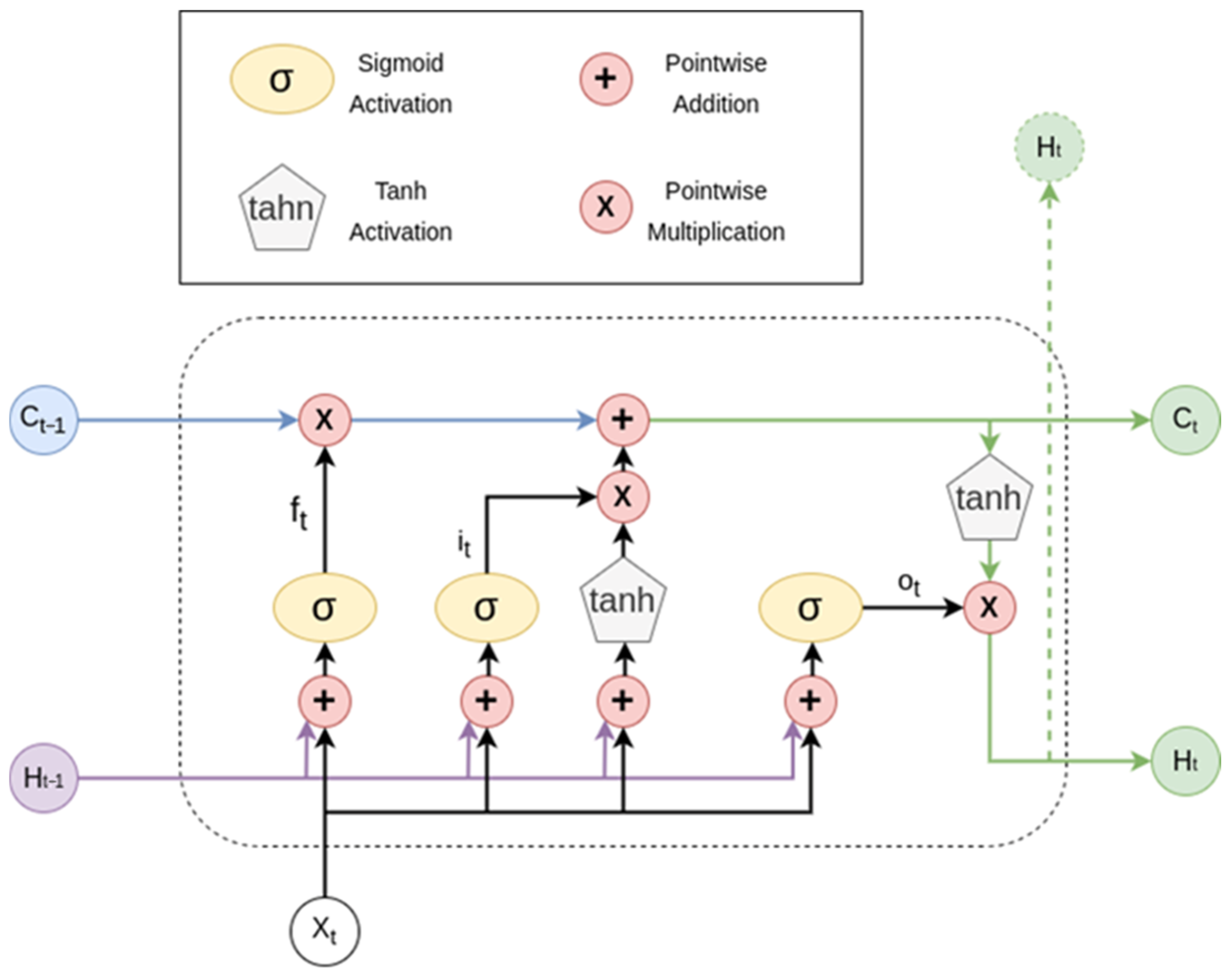
2.1. The Long Short-Term Memory Network
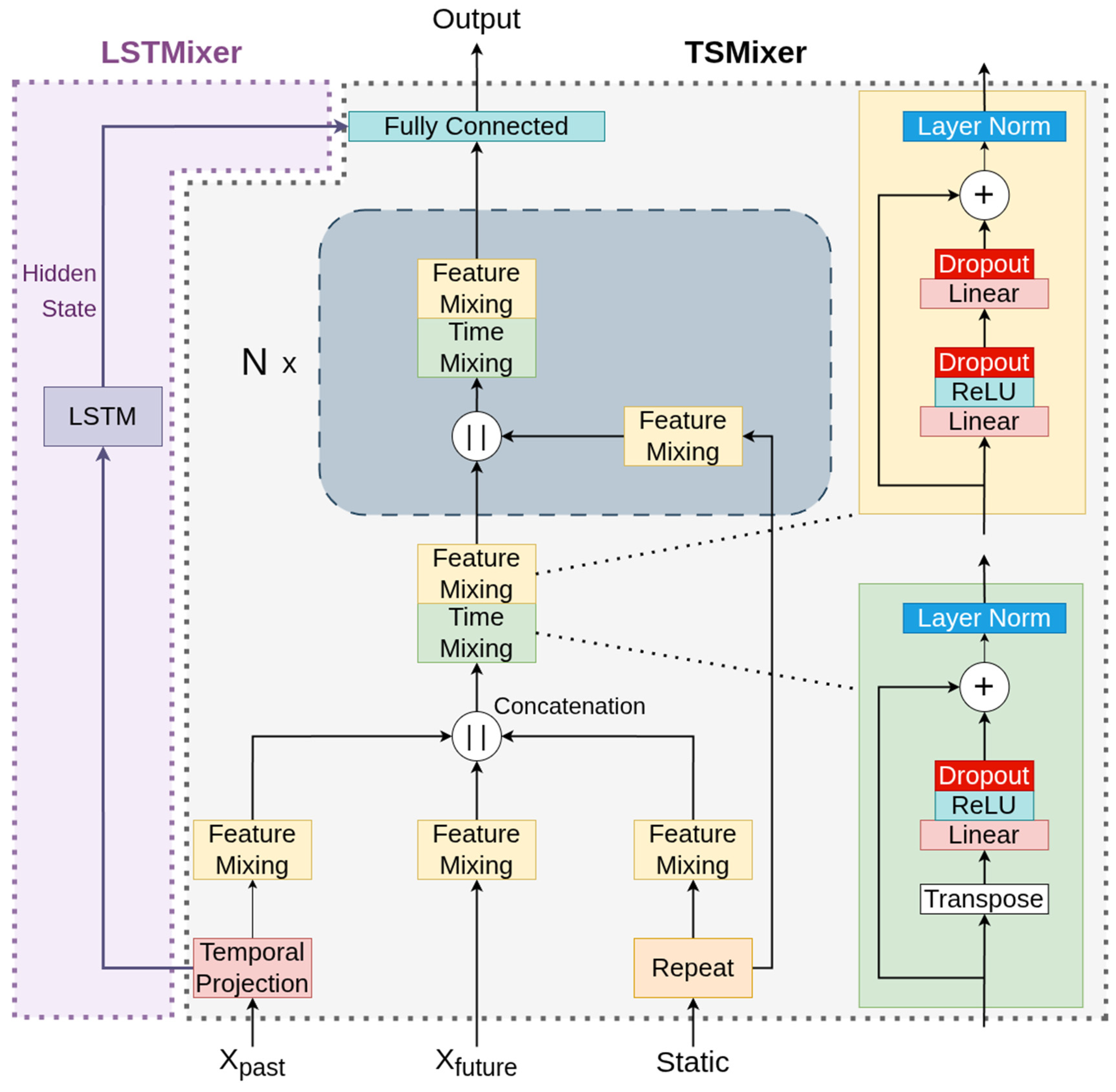
2.2. The Time-Series Mixer and the Proposed LSTMixer
2.3. The Temporal Convolutional Network
- The TCN network is a sequence of multiple Residual Blocks that perform dilated convolutions given a number of kernels k and a dilation factor that exponentially increases, given a base b. The sequence length, m, is automatically calculated so that the network achieves full history coverage.
- Each Residual Block consists of two convolutional layers that are followed by a potential weight normalization, a ReLU activation that enables the model to achieve non-linearity, and a spatial dropout layer.
- Each convolutional layer applies multiple filters given the number of kernels k and dilation factor b.
2.4. The Temporal Fusion Transformer
- Variable selection networks as well as a dedicated static variable encoder to properly handle and filter the input and all covariates that accompany it.
- An LSTM encoder–decoder layer that encapsulates short-term correlations.
- A multi-head attention layer that is able to extract long-term dependencies and benefits from the scalability that Transformer architectures enjoy.
- Multiple residual connections and a dedicated Gated Residual Network (GRN) that skips potentially unnecessary functions within the network
- A final linear layer that is tasked with outputting quantile predictions for probabilistic forecasts whenever such analysis is required.
3. Materials and Methods
3.1. Retail Demand—The Walmart Dataset
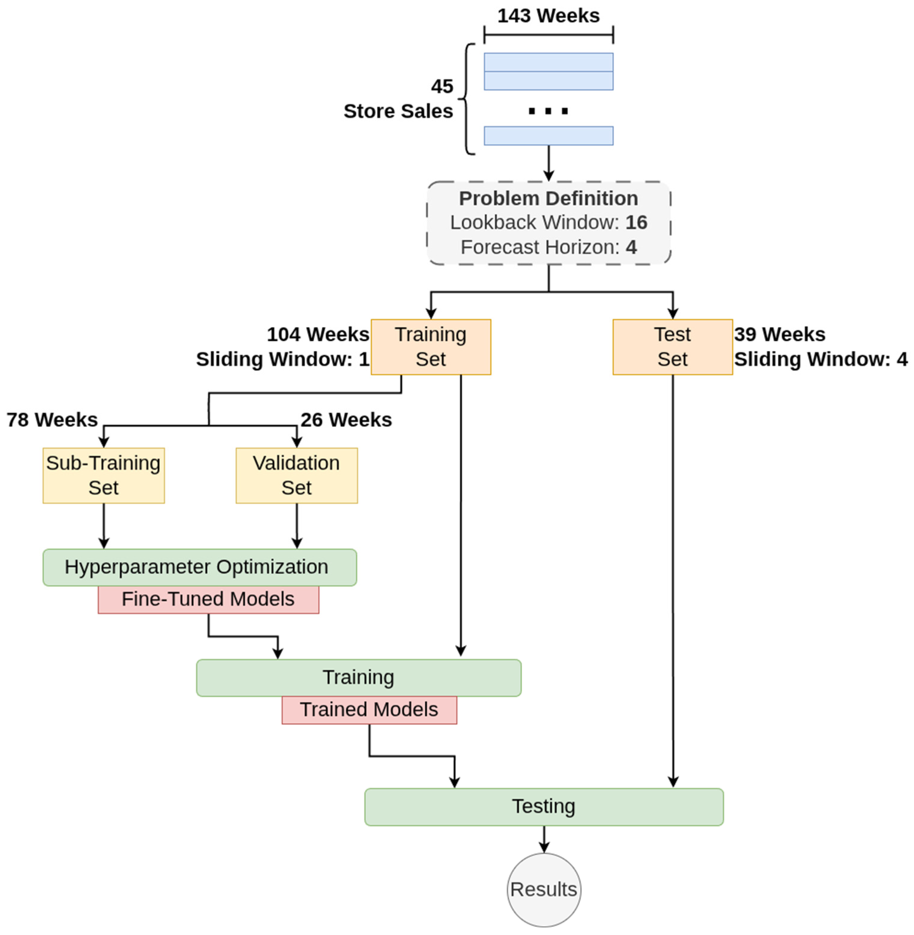
3.2. Problem Definition and Methodology
3.3. Hyperparameter Optimization
4. Results
4.1. Forecasting Results
4.2. LSTMixer Ablation Study
- TSMixer-Pure: By removing the LSTM block altogether a TSMixer model is created with the same parameters as the LSTMixer ones. Hence, the original architecture can be directly compared with the proposed one.
- TSMixer-Pass: The LSTM block is replaced with a linear block that simply transforms the input to match the dimensions of LSTM’s output—the hidden state. This way, the actual benefit of the LSTM block is tested as the TSMixer architecture might generically benefit from this extra connection, that directly passes the unmixed input to the output, regardless of the block used.
5. Discussion
Author Contributions
Funding
Institutional Review Board Statement
Informed Consent Statement
Data Availability Statement
Conflicts of Interest
References
- Eglite, L.; Birzniece, I. Retail sales forecasting using deep learning: Systematic literature review. Complex Syst. Inform. Model. Q. 2022, 30, 53–62. [Google Scholar] [CrossRef]
- Bai, B. Acquiring supply chain agility through information technology capability: The role of demand forecasting in retail industry. Kybernetes 2023, 52, 4712–4730. [Google Scholar] [CrossRef]
- Hwang, T.; Kim, S.T. Balancing in-house and outsourced logistics services: Effects on supply chain agility and firm performance. Serv. Bus. 2019, 13, 531–556. [Google Scholar] [CrossRef]
- Al Humdan, E.; Shi, Y.; Behnia, M.; Najmaei, A. Supply chain agility: A systematic review of definitions, enablers and performance implications. Int. J. Phys. Distrib. Logist. Manag. 2020, 50, 287–312. [Google Scholar] [CrossRef]
- Fildes, R.; Ma, S.; Kolassa, S. Retail forecasting: Research and practice. Int. J. Forecast. 2022, 38, 1283–1318. [Google Scholar] [CrossRef]
- Makridakis, S.; Hyndman, R.J.; Petropoulos, F. Forecasting in social settings: The state of the art. Int. J. Forecast. 2020, 36, 15–28. [Google Scholar] [CrossRef]
- da Veiga, C.P.; da Veiga, C.R.P.; Puchalski, W.; dos Santos Coelho, L.; Tortato, U. Demand forecasting based on natural computing approaches applied to the foodstuff retail segment. J. Retail. Consum. Serv. 2016, 31, 174–181. [Google Scholar] [CrossRef]
- Ghadge, A.; Bag, S.; Goswami, M.; Tiwari, M.K. Mitigating demand risk of durable goods in online retailing. Int. J. Retail Distrib. Manag. 2020, 49, 165–186. [Google Scholar] [CrossRef]
- Gastinger, J.; Nicolas, S.; Stepić, D.; Schmidt, M.; Schülke, A. A study on ensemble learning for time series forecasting and the need for meta-learning. In Proceedings of the 2021 International Joint Conference on Neural Networks (IJCNN), Shenzhen, China, 18–22 July 2021; pp. 1–8. [Google Scholar] [CrossRef]
- Abbasimehr, H.; Shabani, M. A new framework for predicting customer behavior in terms of RFM by considering the temporal aspect based on time series techniques. J. Ambient Intell. Humaniz. Comput. 2021, 12, 515–531. [Google Scholar] [CrossRef]
- Punia, S.; Shankar, S. Predictive analytics for demand forecasting: A deep learning-based decision support system. Knowl.-Based Syst. 2022, 258, 109956. [Google Scholar] [CrossRef]
- Massaoudi, M.; Refaat, S.S.; Chihi, I.; Trabelsi, M.; Oueslati, F.S.; Abu-Rub, H. A novel stacked generalization ensemble-based hybrid LGBM-XGB-MLP model for Short-Term Load Forecasting. Energy 2021, 214, 118874. [Google Scholar] [CrossRef]
- Islam, M.T.; Ayon, E.H.; Ghosh, B.P.; Chowdhury, S.; Shahid, R.; Rahman, S.; Bhuiyan, M.S.; Nguyen, T.N. Revolutionizing retail: A hybrid machine learning approach for precision demand forecasting and strategic decision-making in global commerce. J. Comput. Sci. Technol. Stud. 2024, 6, 33–39. [Google Scholar] [CrossRef]
- Mediavilla, M.A.; Dietrich, F.; Palm, D. Review and analysis of artificial intelligence methods for demand forecasting in supply chain management. Procedia CIRP 2022, 107, 1126–1131. [Google Scholar] [CrossRef]
- Seyedan, M.; Mafakheri, F. Predictive big data analytics for supply chain demand forecasting: Methods, applications, and research opportunities. J. Big Data 2020, 7, 53. [Google Scholar] [CrossRef]
- Torres, J.F.; Hadjout, D.; Sebaa, A.; Martínez-Álvarez, F.; Troncoso, A. Deep learning for time series+ forecasting: A survey. Big Data 2021, 9, 3–21. [Google Scholar] [CrossRef] [PubMed]
- Liu, X.; Wang, W. Deep time series forecasting models: A comprehensive survey. Mathematics 2024, 12, 1504. [Google Scholar] [CrossRef]
- Wen, Q.; Zhou, T.; Zhang, C.; Chen, W.; Ma, Z.; Yan, J.; Sun, L. Transformers in time series: A survey. arXiv 2022, arXiv:2202.07125. [Google Scholar] [CrossRef]
- Lim, B.; Arık, S.Ö.; Loeff, N.; Pfister, T. Temporal fusion transformers for interpretable multi-horizon time series forecasting. Int. J. Forecast. 2021, 37, 1748–1764. [Google Scholar] [CrossRef]
- Bai, S.; Kolter, J.Z.; Koltun, V. An empirical evaluation of generic convolutional and recurrent networks for sequence modeling. arXiv 2018, arXiv:1803.01271. [Google Scholar] [CrossRef]
- Dai, W.; An, Y.; Long, W. Price change prediction of ultra high frequency financial data based on temporal convolutional network. Procedia Comput. Sci. 2022, 199, 1177–1183. [Google Scholar] [CrossRef]
- Ho, R.; Hung, K. Ceemd-based multivariate financial time series forecasting using a temporal fusion transformer. In Proceedings of the 2024 IEEE 14th Symposium on Computer Applications & Industrial Electronics (ISCAIE), Penang, Malaysia, 24–25 May 2024; pp. 209–215. [Google Scholar] [CrossRef]
- Lara-Benítez, P.; Carranza-García, M.; Luna-Romera, J.M.; Riquelme, J.C. Temporal convolutional networks applied to energy-related time series forecasting. Appl. Sci. 2020, 10, 2322. [Google Scholar] [CrossRef]
- Huy, P.C.; Minh, N.Q.; Tien, N.D.; Anh, T.T.Q. Short-term electricity load forecasting based on temporal fusion transformer model. IEEE Access 2022, 10, 106296–106304. [Google Scholar] [CrossRef]
- Hewage, P.; Behera, A.; Trovati, M.; Pereira, E.; Ghahremani, M.; Palmieri, F.; Liu, Y. Temporal convolutional neural (TCN) network for an effective weather forecasting using time-series data from the local weather station. Soft Comput. 2020, 24, 16453–16482. [Google Scholar] [CrossRef]
- Wu, B.; Wang, L.; Zeng, Y.R. Interpretable wind speed prediction with multivariate time series and temporal fusion transformers. Energy 2022, 252, 123990. [Google Scholar] [CrossRef]
- He, Y.; Zhao, J. Temporal convolutional networks for anomaly detection in time series. J. Phys. Conf. Ser. 2019, 1213, 042050. [Google Scholar] [CrossRef]
- Ayhan, B.; Vargo, E.P.; Tang, H. On the exploration of temporal fusion transformers for anomaly detection with multivariate aviation time-series data. Aerospace 2024, 11, 646. [Google Scholar] [CrossRef]
- Zeng, A.; Chen, M.; Zhang, L.; Xu, Q. Are transformers effective for time series forecasting? In Proceedings of the AAAI Conference on Artificial Intelligence, Washington, DC, USA, 7–14 February 2023; Volume 37, No. 9. pp. 11121–11128. [Google Scholar] [CrossRef]
- Das, A.; Kong, W.; Leach, A.; Mathur, S.; Sen, R.; Yu, R. Long-term forecasting with tide: Time-series dense encoder. arXiv 2023, arXiv:2304.08424. [Google Scholar] [CrossRef]
- Chen, S.A.; Li, C.L.; Yoder, N.; Arik, S.O.; Pfister, T. Tsmixer: An all-mlp architecture for time series forecasting. arXiv 2023, arXiv:2303.06053. [Google Scholar] [CrossRef]
- Siami-Namini, S.; Tavakoli, N.; Namin, A.S. The performance of LSTM and BiLSTM in forecasting time series. In Proceedings of the 2019 IEEE International Conference on Big Data (Big Data), Los Angeles, CA, USA, 9–12 December 2019; pp. 3285–3292. [Google Scholar] [CrossRef]
- DiPietro, R.; Hager, G.D. Deep learning: RNNs and LSTM. In Handbook of Medical Image Computing and Computer Assisted Intervention; Academic Press: New York, NY, USA; pp. 503–519. 2020. [Google Scholar] [CrossRef]
- Ba, J.L.; Kiros, J.R.; Hinton, G.E. Layer normalization. arXiv 2016, arXiv:1607.06450. [Google Scholar]
- The Numpy Documentation. Available online: https://numpy.org/ (accessed on 29 May 2025).
- The Pandas Documentation. Available online: https://pandas.pydata.org/ (accessed on 29 May 2025).
- The Scikit-Learn Documentation. Available online: https://scikit-learn.org/stable/ (accessed on 29 May 2025).
- The XGBoost Documentation. Available online: https://xgboost.readthedocs.io/en/stable/ (accessed on 29 May 2025).
- The PyTorch Documentation. Available online: https://pytorch.org/ (accessed on 29 May 2025).
- The Walmart Sales Forecast Dataset. Available online: https://www.kaggle.com/datasets/aslanahmedov/walmart-sales-forecast?select=train.csv (accessed on 29 May 2025).
- Trauzettel, V. Optimal stocking of retail outlets: The case of weekly demand pattern. Bus. Logist. Mod. Manag. 2014, 14, 3–11. [Google Scholar]
- The Optuna Documentation. Available online: https://optuna.readthedocs.io/en/stable/index.html (accessed on 29 May 2025).
- Watanabe, S. Tree-structured parzen estimator: Understanding its algorithm components and their roles for better empirical performance. arXiv 2023, arXiv:2304.11127. [Google Scholar] [CrossRef]
- Li, L.; Jamieson, K.; DeSalvo, G.; Rostamizadeh, A.; Talwalkar, A. Hyperband: A novel bandit-based approach to hyperparameter optimization. J. Mach. Learn. Res. 2018, 18, 1–52. [Google Scholar]
- Kingma, D.P. Adam: A method for stochastic optimization. arXiv 2014, arXiv:1412.6980. [Google Scholar] [CrossRef]
- Chen, T.; Guestrin, C. Xgboost: A scalable tree boosting system. In Proceedings of the 22nd ACM SIGKDD International Conference on Knowledge Discovery and Data Mining, San Francisco, CA, USA, 13–17 August 2016; pp. 785–794. [Google Scholar] [CrossRef]
- Vinayak, R.K.; Gilad-Bachrach, R. Dart: Dropouts meet multiple additive regression trees. In Proceedings of the Artificial Intelligence and Statistics, San Diego, CA, USA, 9–12 May 2015; pp. 489–497. [Google Scholar]
- Dhamo, E.; Puka, L. Using the R-package to forecast time series: ARIMA models and Application. In Proceedings of the International Conference Economic & Social Challenges and Problems, Tiranë, Albania, 10 December 2010; pp. 1–14. [Google Scholar]
- Harvey, D.; Leybourne, S.; Newbold, P. Testing the equality of prediction mean squared errors. Int. J. Forecast. 1997, 13, 281–291. [Google Scholar] [CrossRef]


| Covariate | Explanation | Type |
|---|---|---|
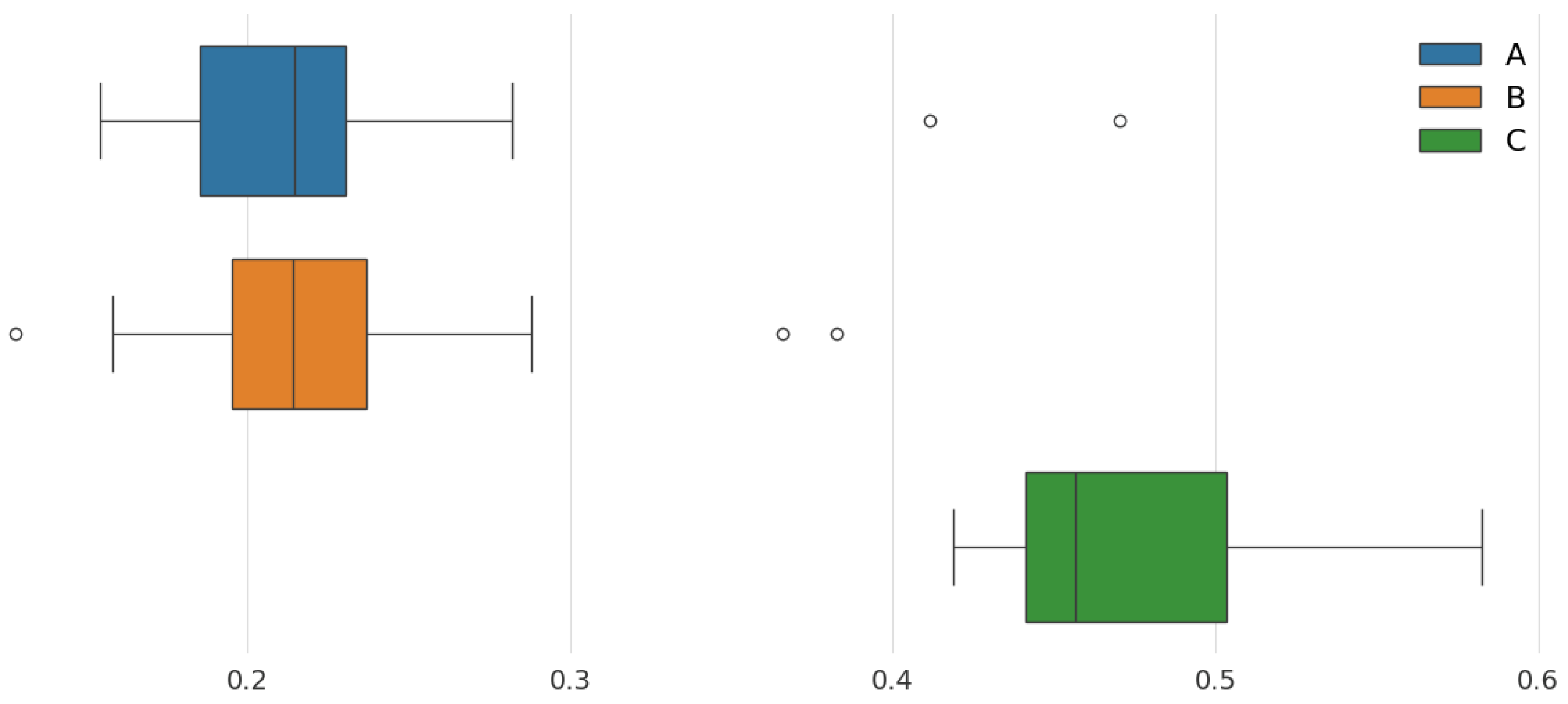
| Type | The anonymized type of the store as A, B or C. | Static |
| Size | The size of the store. | Static |
| Temperature | The average temperature in the area. | Past |
| Fuel_Price | The average fuel price in the area. | Past |
| CPI | The consumer price index. | Past |
| Unemployment | The unemployment rate. | Past |
| isHoliday | This declares if the current week is/contains a holiday. | Future |
| MarkDown 1–5 (5 separate features) | Special ongoing promotions. | Future |
| Metric | Value |
|---|---|
| Mean | 0.26 |
| Std | 0.18 |
| 25% Percentile | 0.14 |
| Median | 0.20 |
| 75% Percentile | 0.33 |
| Model | Hyperparameters | Values |
|---|---|---|
| XGBoost | Dropout rate | 0, 0.1, 0.2, 0.3 |
| Learning rate | 10−1, 10−2, 10−3, 10−4 | |
| Hessian | 0.5, 1, 2 | |
| Gamma | 1, 10−1, 10−2, 10−3 | |
| Max depth | 4, 8, 16, None | |
| LSTM | Hidden map size | 16, 32, 64, 128 |
| Number of LSTM stacks | 1, 2, 4, 8 | |
| Number of hidden layers in FC | 2, 4, 8 | |
| Number of neurons per layer in FC | 8, 16, 32, 64 | |
| Dropout rate | 0, 0.1, 0.2, 0.3 | |
| Learning rate | 10−1, 10−2, 10−3, 10−4 | |
| Batch size | 4, 8, 16, 32 | |
| TSMixer | Number of mixing rounds | 2, 4, 8, 16 |
| Size of first layer in FM | 32, 64, 128 | |
| Size of second layer in FM | 32, 64, 128 | |
| Dropout rate | 0, 0.1, 0.2, 0.3 | |
| Learning rate | 10−1, 10−2, 10−3, 10−4 | |
| Batch size | 4, 8, 16, 32 | |
| LSTMixer | Number of mixing rounds | 2, 4, 8, 16 |
| Size of first layer in FM | 32, 64, 128 | |
| Size of second layer in FM | 32, 64, 128 | |
| Hidden map size | 16, 32, 64, 128 | |
| Number of LSTM stacks | 1, 2, 4, 8 | |
| Dropout rate | 0, 0.1, 0.2, 0.3 | |
| Learning rate | 10−1, 10−2, 10−3, 10−4 | |
| Batch size | 4, 8, 16, 32 | |
| TCN | Kernel size | 2, 4, 8 |
| Number of filters | 2, 4, 8 | |
| Dilation base | 2, 3, 4 | |
| Dropout rate | 0, 0.1, 0.2, 0.3 | |
| Learning rate | 10−1, 10−2, 10−3, 10−4 | |
| Batch size | 4, 8, 16, 32 | |
| TFT | Hidden state size | 16, 32, 64, 128 |
| Number of LSTM stacks | 1, 2, 4, 8 | |
| Number of attention heads | 2, 4, 8 | |
| Dropout rate | 0, 0.1, 0.2, 0.3 | |
| Learning rate | 10−1, 10−2, 10−3, 10−4 | |
| Batch size | 4, 8, 16, 32 |
| Model | sMAPE | MAE | RMSE |
|---|---|---|---|
| LSTMixer | 18.8 | 0.041 | 0.050 |
| 21.7 | 0.046 | 0.059 | |
| TFT | 19.8 | 0.042 | 0.052 |
| 22.9 | 0.047 | 0.060 | |
| TCN | 20.4 | 0.046 | 0.060 |
| 23.5 | 0.051 | 0.067 | |
| TSMixer | 22.2 | 0.045 | 0.059 |
| 25.2 | 0.054 | 0.070 | |
| XGBoost | 23.1 | 0.043 | 0.053 |
| 26.2 | 0.054 | 0.068 | |
| LSTM | 22.9 | 0.050 | 0.060 |
| 27.5 | 0.056 | 0.071 | |
| SARIMA | 24.5 | 0.051 | 0.064 |
| 28.1 | 0.058 | 0.072 | |
| ETS | 28.4 | 0.069 | 0.088 |
| 30.3 | 0.069 | 0.091 |
| LSTMixer | TFT | TCN | TSMixer | |
|---|---|---|---|---|
| LSTMixer | - | 0.049 | 0.049 | 0.037 |
| - | 0.047 | 0.046 | 0.042 | |
| TFT | 0.049 | - | 0.073 | 0.035 |
| 0.047 | - | 0.070 | 0.044 | |
| TCN | 0.049 | 0.073 | - | 0.048 |
| 0.046 | 0.070 | - | 0.049 | |
| TSMixer | 0.037 | 0.035 | 0.048 | - |
| 0.042 | 0.044 | 0.049 | - | |
| XGBoost | 0.039 | 0.049 | 0.049 | 0.050 |
| 0.042 | 0.046 | 0.046 | 0.046 |
| Model | sMAPE | MAE | RMSE | p-Values |
|---|---|---|---|---|
| LSTMixer | 18.8 | 0.041 | 0.050 | - |
| 21.7 | 0.046 | 0.059 | - | |
| TSMixer-Pure | 22.8 | 0.042 | 0.060 | 0.045 |
| 25.9 | 0.054 | 0.068 | 0.043 | |
| TSMixer-Pass | 25.8 | 0.051 | 0.059 | 0.045 |
| 27.8 | 0.057 | 0.070 | 0.040 |
Disclaimer/Publisher’s Note: The statements, opinions and data contained in all publications are solely those of the individual author(s) and contributor(s) and not of MDPI and/or the editor(s). MDPI and/or the editor(s) disclaim responsibility for any injury to people or property resulting from any ideas, methods, instructions or products referred to in the content. |
© 2025 by the authors. Licensee MDPI, Basel, Switzerland. This article is an open access article distributed under the terms and conditions of the Creative Commons Attribution (CC BY) license (https://creativecommons.org/licenses/by/4.0/).
Share and Cite
Theodoridis, G.; Tsadiras, A. Retail Demand Forecasting: A Comparative Analysis of Deep Neural Networks and the Proposal of LSTMixer, a Linear Model Extension. Information 2025, 16, 596. https://doi.org/10.3390/info16070596
Theodoridis G, Tsadiras A. Retail Demand Forecasting: A Comparative Analysis of Deep Neural Networks and the Proposal of LSTMixer, a Linear Model Extension. Information. 2025; 16(7):596. https://doi.org/10.3390/info16070596
Chicago/Turabian StyleTheodoridis, Georgios, and Athanasios Tsadiras. 2025. "Retail Demand Forecasting: A Comparative Analysis of Deep Neural Networks and the Proposal of LSTMixer, a Linear Model Extension" Information 16, no. 7: 596. https://doi.org/10.3390/info16070596
APA StyleTheodoridis, G., & Tsadiras, A. (2025). Retail Demand Forecasting: A Comparative Analysis of Deep Neural Networks and the Proposal of LSTMixer, a Linear Model Extension. Information, 16(7), 596. https://doi.org/10.3390/info16070596